Inclusion of Hydraulic Controls in Rehabilitation Models of Drainage Networks to Control Floods

Abstract

A problem for drainage systems managers is the increase in extreme rain events that are increasing in various parts of the world. Their occurrence produces hydraulic overload in the drainage system and consequently floods. Adapting the existing infrastructure to be able to receive extreme rains without generating consequences for cities’ inhabitants has become a necessity. This research shows a new way to improve drainage systems with minimal investment costs, using for this purpose a novel methodology that considers the inclusion of hydraulic control elements in the network, the installation of storm tanks and the replacement of pipes. The presented methodology uses the Storm Water Management Model for the hydraulic analysis of the network and a modified Genetic Algorithm to optimize the network. In this algorithm, called the Pseudo-Genetic Algorithm, the coding of the chromosomes is integral and has been used in previous studies of hydraulic optimization. This work evaluates the cost of the required infrastructure and the damage caused by floods to find the optimal solution. The main conclusion of this study is that the inclusion of hydraulic controls can reduce the cost of network rehabilitation and decrease flood levels.

1. Introduction

Discussions have been generated about the pressure that climate change can generate on water supply and drainage systems. Recent research has shown that climate change is a preponderant factor and affects the future availability of water resources [1]. Additionally, other studies show that due to anthropogenic climate change, the climate cannot be considered unchanging and presents spatially heterogeneous trends in both mean behavior and variability. [2] This shows that the increase in extreme rains in certain parts of the world is evident, and there is a need to take measures [3]. Floods in urban areas are mainly due to the increase in the impervious surface and the increase in the intensity of extreme rains [4,5,6,7]. This increase and the impervious surface due to the urban growth of cities reduces the time of concentration of the water and produces a rapid accumulation of water on the surface that drainage network systems cannot evacuate. All these effects have a consequence: the appearance of increasingly frequent and intense floods.

Floods in urban areas are one of the problems of greatest concern. The damage associated with this type of disaster is expected to increase in the future [8,9]. Although rain floods generate less economic losses than river floods, they are much more frequent, so their accumulated cost could be higher in one year than another [10].

There are different methods or technologies that can be applied to face the consequences of excess runoff in urban areas. A proven measure to control urban runoff is the installation of infrastructure that allows water to be temporarily retained and stored during rain events. One of the best structures to achieve this goal is Storm Tanks (STs). In this field, one of the first works was developed by Howard [11], who presented a theoretical method to evaluate the storage efficiency of a retention tank in combination with a treatment plant using probabilistic methods based on precipitation data. More recently, Butler et al. [12] studied the effect of climate change on ST performance. They relied on Intergovernmental Panel on Climate Change (IPCC) medium-high emission scenarios for the city of London. The results of their work indicate that significantly larger storage volumes are required to maintain the same level of flood protection. One of the most prominent studies on this topic was conducted by Andrés-Doménech et al. [13], who studied the ability of STs to regain their efficiency. With this objective, they presented a probabilistic analytical model to assess the volumetric efficiency of STs according to the new climatic scenarios and urban catchment.

Later, Wang et al. [14] presented a method of optimizing the location of STs in two modules trying to reduce flooding, cost of tanks and available total solids load. The first module evaluates and classifies flood nodes with the Analytical Hierarchy Process (AHP) [15] using two indicators: flood depth and flood duration. The second is an iterative module that provides the optimal scheme for the location of the tanks through the method of searching for generalized patterns. In addition, Cunha et al. [16] presented an optimization method based on a previous disposition of STs to size them and the outflow orifice. They concluded the importance of a good dimensioning of the orifice since it reduces the output flow of the storage unit that regulates the descending flows, allowing flow control and a reduction of floods in the whole network.

Better results are obtained by the combination of STs and the replacement of pipes with others with higher diameters. Saldarriaga et al. [17] applied two different approaches to determine the optimal location and size of the storage units through the application of Simulated Annealing and Genetic Algorithms. This research validated the use of STs for peak flow reduction in urban areas. It also showed the advantages of considering the replacement of certain pipes and the installation of STs instead of replacing the whole pipe infrastructure. Iglesias et al. [18] presented a methodology to improve stormwater systems using an optimization model that incorporates a Pseudo Genetic Algorithm (PGA) [19]. The model includes as decision variables the replacement of pipes, the location and sizing of STs and the initial state, and start and stop levels in the case of systems with pumping stations. The study demonstrated the economic benefits of the joint installation of STs and the replacement of pipes with others of greater capacity. Following this line of research, Ngamalieu-Nengoue et al. [20] present a methodology that uses the aforementioned postulates seeking rehabilitation of drainage networks and shortens the calculation time through a process of Search Space Reduction (SSR). Their methodology is divided into two parts. The first one uses a PGA and aims to reduce the search space for solutions. The second one optimizes the multiple objectives of the new scenario generated in the first part using a Non-dominated Sorting Genetic Algorithm (NSGA-II). Continuing with his research, Ngamalieu-Nengoue et al. [21] present in their work a way to calculate the flood level using the ponded area of the Storm Water Management Model (SWMM) [22]. The optimization model assumes the definition of this area in each node to convert flood volume into flood level. The method developed by Ngamalieu-Nengoue et al. [21] considers reducing the diameter of certain pipes and concludes that it is necessary to include resistance elements that generate a head loss equivalent to that which would be caused by the installation of smaller diameters.

The use of hydraulic controls in drainage networks is considered by different authors as a tool to limit the flow of water in drainage networks, promoting their retention and storage within the network. An outstanding study is the one prepared by Dziopak [23], who proposed, as an alternative to ST, using the sewerage network as a temporary water storage unit. To achieve this goal, this author designed a retention channel with interior partitions in the form of cameras with an opening at the bottom of the channel acting as an orifice. In this way, the conduit becomes a retention channel.

On the other hand, Leitão et al. [24] presented a model that includes an algorithm for the location of flow limiters in the drainage network with the objective of maximizing storage within the network. They reach two conclusions. The first was that the storage capacity in the networks can be very large. The second was that if the local flow control devices are installed correctly, it can become an interesting solution to mitigate floods. This model also considers the potential impact of the failure of the flow control device. In parallel, Słyś [25] proposed a type of channel to retain runoff within the network. To achieve this, the channel is segmented into compartments. These compartments have two outlets; a hole at the bottom for the passage of wastewater and an opening at the top to allow rainwater to overflow into the next compartment. Later, Ngamalieu-Nengoue et al. [26] obtained optimized diameters smaller than the original in certain pipes as a result of their study in which they use an NSGA-II. These results emphasize the need to include hydraulic controls to introduce a head loss in the system. These investigations suggest that hydraulic controls can be used as a technique to improve the efficiency of the system by allowing the accumulation of water at certain points in the network. Hydraulic controls slow down the flow of the water, reducing the concentration time and therefore the probability of flooding. However, none of the previous authors has considered performing joint optimization of STs and hydraulic controls.

For this reason, this methodology proposes including the use of hydraulic control in the optimization of drainage networks. In this work, two classes of cost functions have been defined, one associated with the investment cost to improve the network (installation of tanks, replacement of pipes and elements for hydraulic control) and the other related to the cost of the damage that flooding can cause. To find the optimal solution, the model uses a PGA connected to the SWMM hydraulic simulation model through a Toolkit [27]. For this reason, the objective of this work is to include additional energy losses to help retain water in the network, decrease the levels of flooding in the networks and minimize the size of the necessary protection structures.

2. Formulation of the Problem

2.1. Initial Assumtions

The methodology consists of performing the hydraulic analysis of the network using the SWMM model and with the help of a PGA to find the best solutions to adapt the system to extreme rain events. The possibilities to improve the performance of the network are changing pipe diameters, installing ST and including devices for hydraulic control of flow. Presented in this way, the following hypotheses are considered:

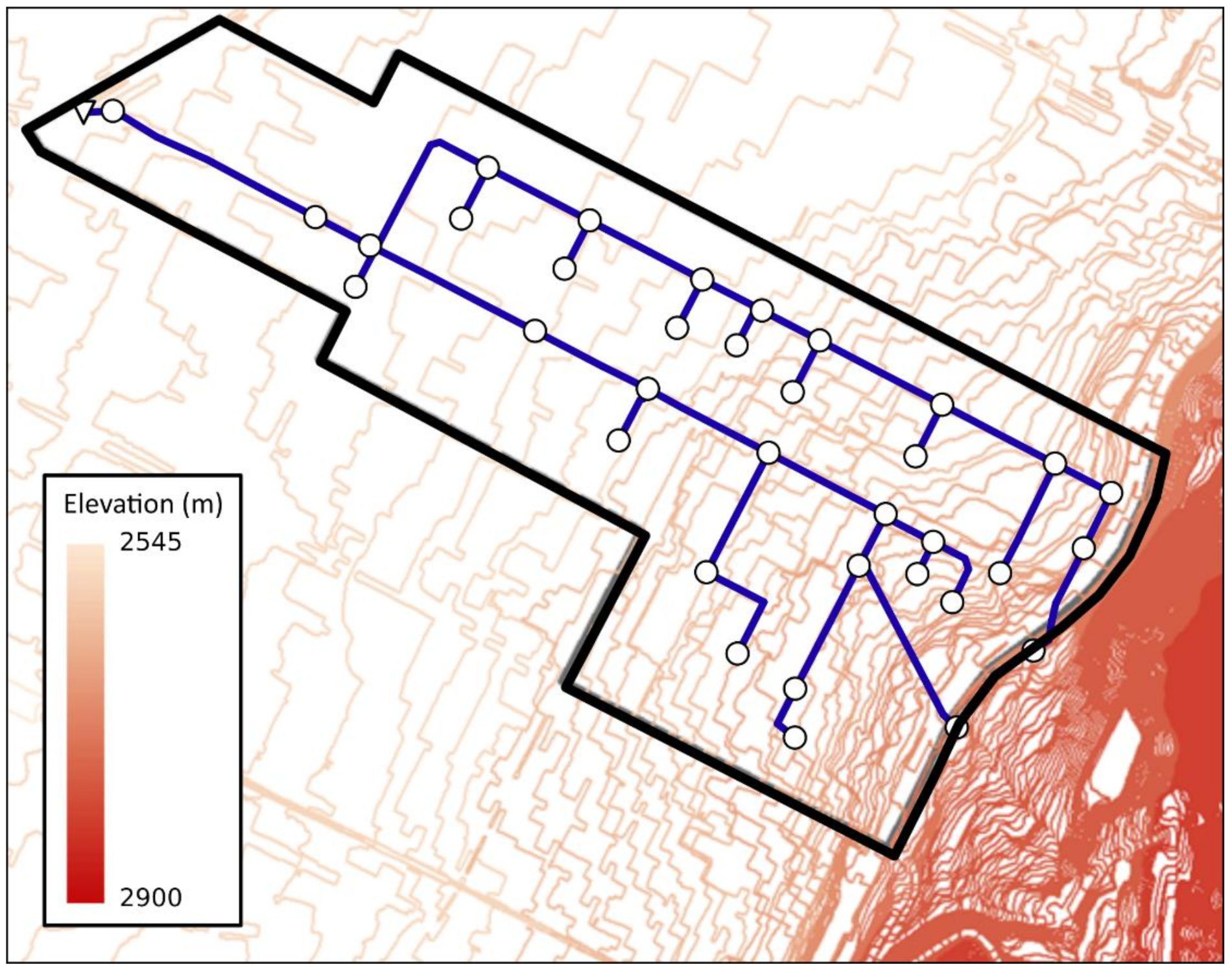
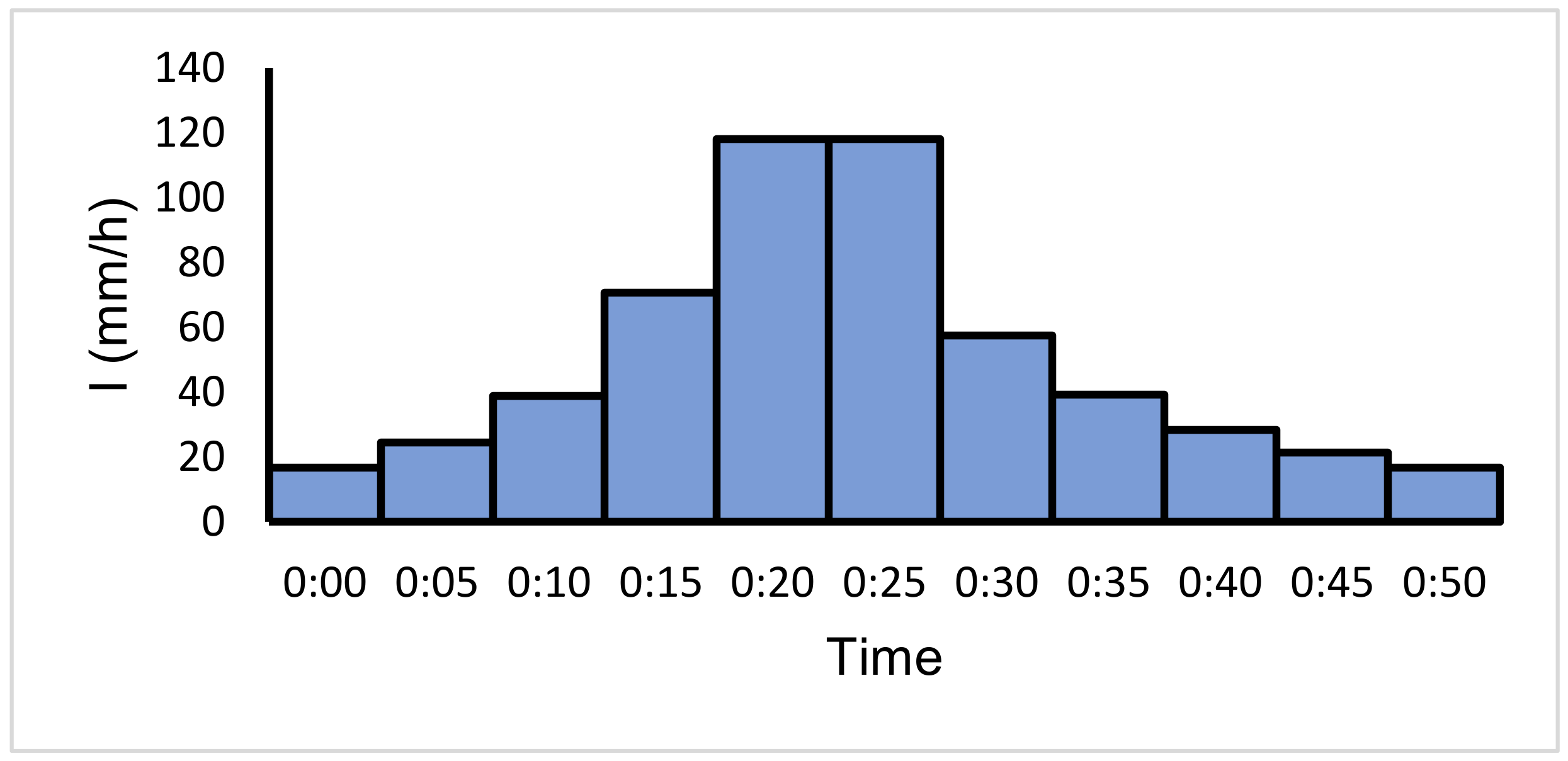
• A spatially static design storm is considered for the entire network. This design storm contemplates the most unfavorable operating scenario. The hydrologic study and the runoff model are beyond the scope of this work. Usually, for design or assessment purposes in small, urban areas, flash floods are used as defined by Merz and Blöschl [28].
• The SWMM is used as a network analysis tool. Dynamic wave model was used because it is the model that best represents both the pressurized flow and floods.
• The mathematical model of the network must be calibrated and simplified as much as possible without losing accuracy in the results.
• The actions considered are the renovation of pipes with others of greater diameter, the installation of STs and the installation of hydraulic controls. Changes in the topology of the network are not included in this work.
• STs are considered installed on-line, and their depth is the same as that of the existing manhole. Therefore, the cost of STs is proportional to the depth, and the area of STs is defined as a decision variable.
• The optimization problem is analyzed in terms of costs [21]. The objective function must be established based on the hydraulic variables and includes the cost of renovating pipes, the cost of installing STs, the cost of hydraulic controls and the damage costs caused by floods.

2.2. Hydraulic Control

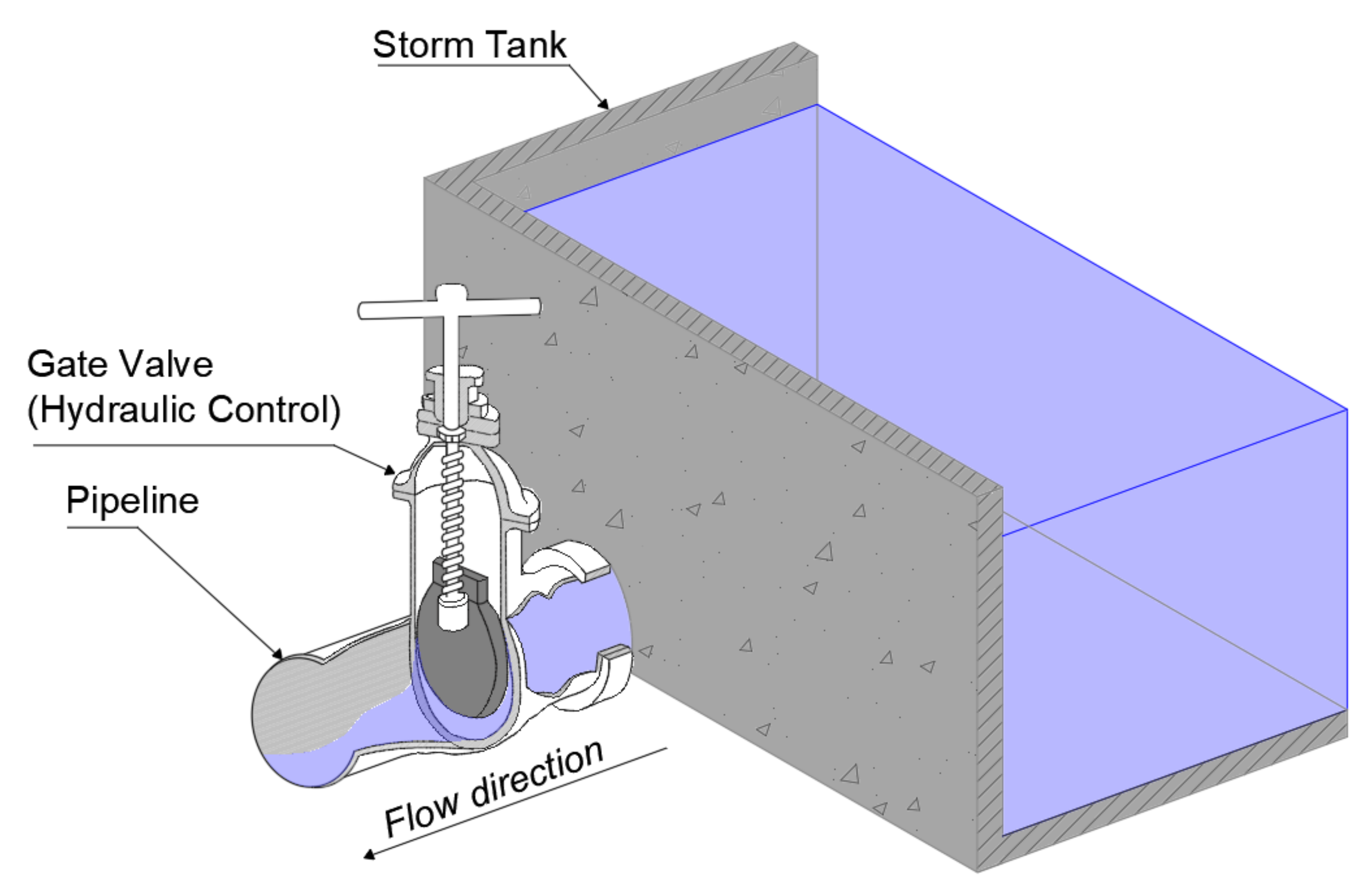
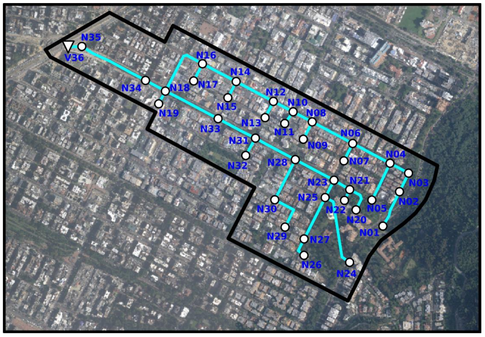
A hydraulic control element is a device that allows the control of flow in the network. In this work, the hydraulic controls are installed in the pipes that come out of the STs (Figure 1). The purpose of including this device is to generate a local loss to slow down the flow of water, inducing it to accumulate upstream and using the network as temporary storage. This alternative is presented as a novel option that can contribute to improving the levels of flooding of the networks and minimizing the size of the necessary protection infrastructure.

In the results obtained in the study carried out by Ngamalieu-Nengoue et al. [21], the reduction of the diameter is observed in certain pipes leaving ST. These smaller diameters act as hydraulic control in the system. It would then be thought that the inclusion of a local head loss in the initial part of the pipe that leaves the ST produces similar results to those obtained by these researchers. This statement needed to be proven.

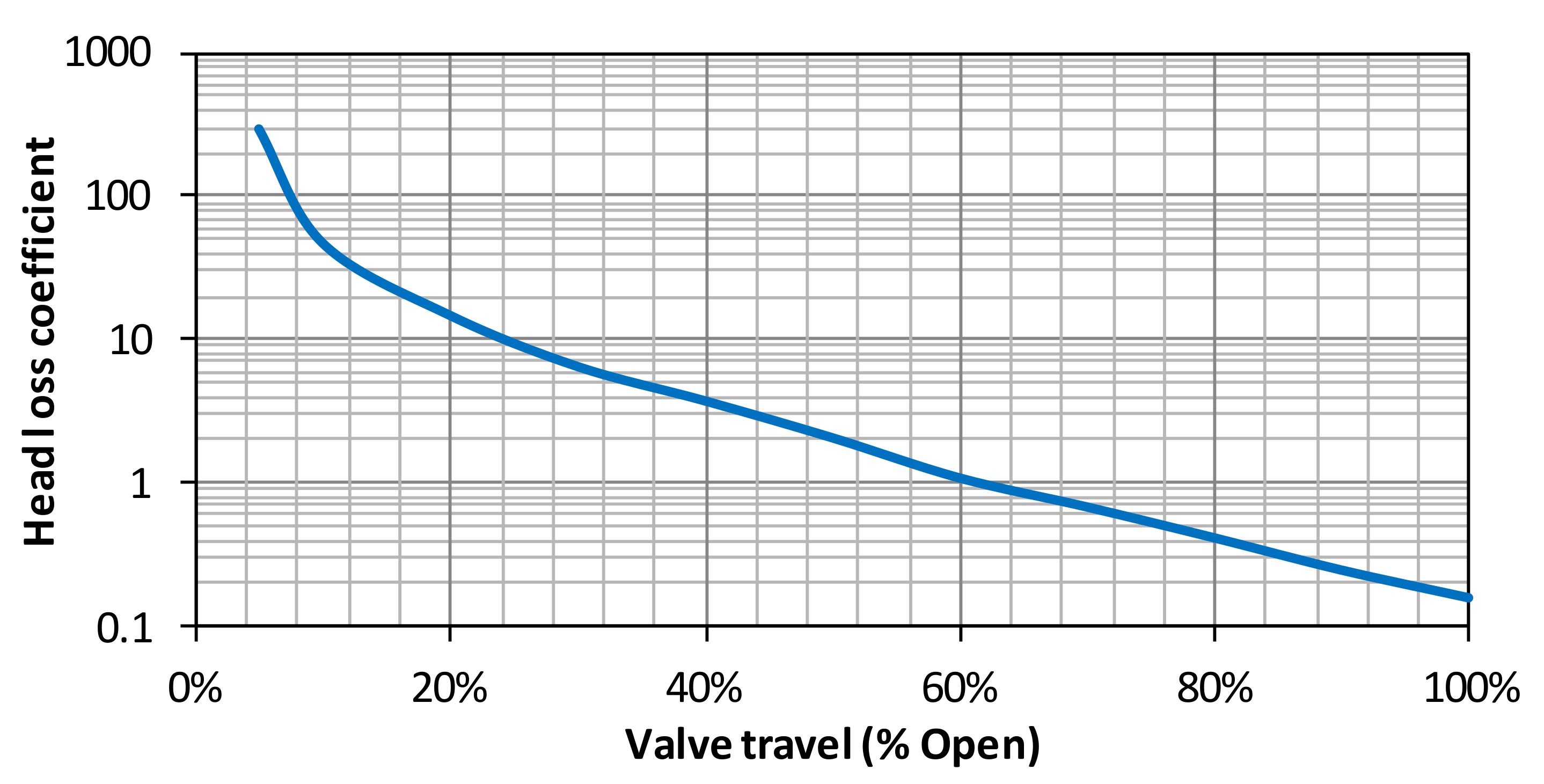
To find the best option for including the hydraulic controls, the network used by Ngamalieu-Nengoue et al. [21] was used. In the final solution presented by these authors, it was observed that two pipes of the solution (named as P04 and P10) had smaller diameters than the original ones. Reducing diameters during a rehabilitation program in a sewage network seemed unrealistic. An alternative solution consisted of the use of some type of hydraulic control of flow in these pipes. To verify that similar results could be obtained, the network was considered with the optimized solution proposed by the authors but keeping the original diameters of pipes P04 and P10. In these pipes, a hydraulic control based on including local head losses was used. This local loss was modeled by installing a valve or a gate in the initial part of the pipes that came out of the ST. The area of the through-hole is variable, allowing setting the opening according to the demands of the system. To represent the head loss generated by the control element, an expression to calculate the coefficient of losses in valves was needed. In this work, the expression defined by Tullis [29] was used (Equation (1)):

$$\mathrm{k}=\frac{2\mathrm{g}\Delta \mathrm{H}}{{\mathrm{V}}^2}$$

(1)

where, g is the acceleration of the gravity, ΔH is the loss of energy in the gate and V is the average flow velocity through the gate. The values of the coefficient k as a function of valve travel are shown in Figure 2.

The head loss coefficient represented in Figure 2 can be mathematically adjusted to the following Equation (2):

$$\mathrm{k}={\mathrm{C}}_1{\mathsf{\theta }}^{{\mathrm{C}}_2}$$

(2)

where C₁ and C₂ represent the adjustment coefficients and θ is the valve opening percentage. For this work, the value used of coefficient C₁ was 0.2736 and the value for the exponent C₂ was −2.395.

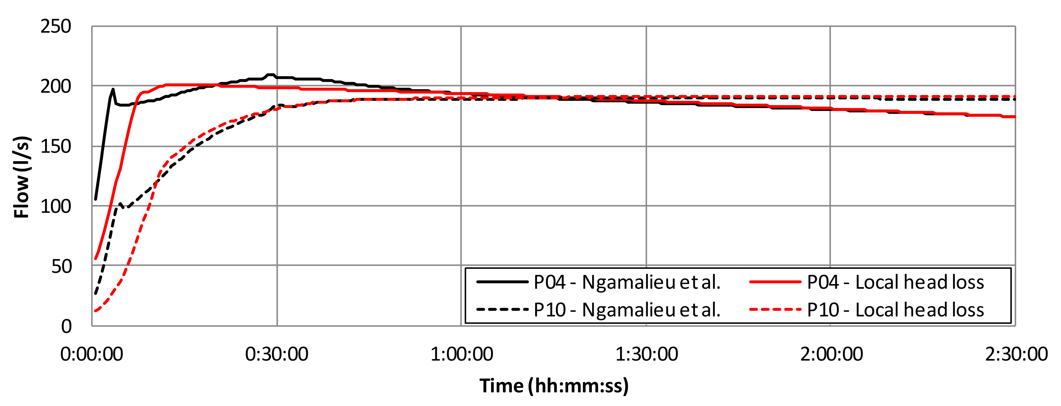
The local head loss defined in Equation (1) was calculated based on the flow that the pipes with the smaller diameter would transport. Once these local head losses were obtained, they were included in pipes P04 and P10. Under these conditions, a hydraulic analysis of the network was performed in the SWMM model, obtaining the flow rates in these pipes for the entire simulation period. Figure 3 compares the flow rates of the pipes P04 and P10 in the solution presented by Ngamalieu-Nengoue et al. [21] to the flow rates that were obtained including a local head loss in the pipes.

The results indicated that both alternatives (a pipe with a reduced diameter and a local head loss) could be used as Hydraulic Control in a network. It is interesting to analyze the use of a local loss since it would be much easier to implement than a pipe change and economically more advantageous. In the work presented in this paper, a modification of the SWMM connection Toolkit was done to allow the modification of the local head loss coefficient within any pipe.

2.3. Decision Variables

In this investigation, the drainage network optimization problem considers three types of decision variables. The first type is the diameter of the pipes; the optimization model searches for the best combination of network diameters to minimize flooding. This decision variable can range from a value of 0 (the pipe is not replaced) to a maximum established value. The value 0 implies that the capacity of the pipe is enough to carry the analyzed flow, while a different value indicates the need to increase the capacity of the pipe. It is necessary to define the following parameters for the analysis of this decision variable: N_C represents the number of pipes in the network, and m_s is the number of pipes selected for replacement and can vary from 0 to N_C. Each pipe candidate to be replaced can adopt a diameter of a defined range. Therefore, ND is defined as the range of available diameters, and this range can have a reduced number of diameters ND₀ or a full range ND_max.

The second type of decision variable considered by the optimization model is the storage capacity of the nodes. The optimization model searches for the best location of the STs in the network and their lowest volume to reduce flooding. When considering the problem in an urban environment, the excavation is limited to the current depth of the manholes, defining the cross-section of the ST as a decision variable. Decision variables related to STs can take values from 0 (ST is not required in the node) to a previously defined maximum value based on the available space. The model defines the following parameters to analyze this decision variable: N_N is the number of nodes in the network; n_s is the number of nodes where ST will be installed and whose value can vary from 0 to N_N. SWMM defines the cross-section of an ST using Equation (3):

$$\mathrm{S}={\mathrm{A}}_{\mathrm{S}}{\mathrm{y}}^{{\mathrm{B}}_{\mathrm{S}}}+{\mathrm{C}}_{\mathrm{S}}$$

(3)

where A_S, B_S and C_S are adjustment coefficients for the tank section and y is the water level of the node. For tanks of constant section, the coefficient A_S represents the cross-section, while the coefficients B_S and C_S are null. This cross-section S must necessarily be discretized. For this purpose, the maximum cross-section S_max is divided into a range of partitions N that can take values from N₀ to N_max.

The last group of decision variables are those that consider the loss coefficients introduced in certain pipes in the network. A local loss can be caused by a rapid change in magnitude or direction of velocity (bends, contractions or extensions in the pipe geometry). In this work, a gate valve with different opening degrees is installed in the initial part of the pipes that come out of the ST. The action of this local head loss is considered as hydraulic control. The number of pipes in which hydraulic controls are installed is represented by p_s. θ is defined as the opening range that the gate valve can adopt. The range of opening values that the gate valve can take is represented as Nθ.

2.4. Objective Function

The objective function to be optimized is established in monetary units and is based on the research carried out by Ngamalieu-Nengoue et al. [20]. The main contribution of this work is to consider a new term in the objective function. This term is the cost function of installation of the hydraulic control elements at the exit of the selected STs. Equation (4) represents the objective function.

$$\mathrm{F}={\mathsf{\tau }}_1{\displaystyle \sum }_{\mathrm{i}=1}^{{\mathrm{m}}_{\mathrm{s}}}{\mathrm{C}}_{\mathrm{D}}\left({\mathrm{D}}_{\mathrm{i}}\right)+{\mathsf{\tau }}_2{\displaystyle \sum }_{\mathrm{i}=1}^{{\mathrm{n}}_{\mathrm{s}}}{\mathrm{C}}_{\mathrm{V}}\left({\mathrm{V}}_{\mathrm{i}}\right)+{\mathsf{\tau }}_3{\displaystyle \sum }_{\mathrm{i}=1}^{{\mathrm{p}}_{\mathrm{s}}}{\mathrm{C}}_{\mathrm{v}}\left({\mathrm{D}}_{\mathrm{i}}\right)+{\mathsf{\tau }}_4{\displaystyle \sum }_{\mathrm{i}=1}^{{\mathrm{N}}_{\mathrm{N}}}{\mathrm{C}}_{\mathrm{y}}\left({\mathrm{y}}_{\mathrm{i}}\right)$$

(4)

where C_D(D_i) represents the cost of the renovation of pipes, C_V(V_i) represents the cost of installation of the STs, C_v(D_i) represents the cost of the installation of the hydraulic control and C_y(y_i) represents the damage costs caused by the flood.

The cost of the renovation of the pipes was established from actual data supplied by manufacturers. This function represents the cost of changing pipes for others of greater capacity. It is a second-degree polynomial function and is expressed as a function of the diameter D Equation (5) expresses the cost of each meter of pipe. In this equation, α and β are adjustment coefficients selected for each project.

$${\mathrm{C}}_{\mathrm{D}}\left({\mathrm{D}}_{\mathrm{i}}\right)=\propto {\mathrm{D}}_{\mathrm{i}}+{\mathsf{\beta }\mathrm{D}}_{\mathrm{i}}{}^2$$

(5)

The cost of installing ST is related to the volume required to store water that cannot be evacuated by the network in an event of extreme rain. The cost function (Equation (6)) is composed of two terms. The first term, C_min, represents a minimum cost established for the ST, while the second term, V_j, is variable based on the required storage volume V_j affected by a constant C_var and an exponent w.

$${\mathrm{C}}_{\mathrm{V}}\left({\mathrm{V}}_{\mathrm{i}}\right)={\mathrm{C}}_{\min }+{\mathrm{C}}_{\mathrm{var}}{\mathrm{V}}_{\mathrm{i}}{}^{\mathsf{\omega }}$$

(6)

The cost of installing hydraulic control was established based on the actual cost of gate valves of different diameters supplied by the manufacturers. It is a second-degree polynomial function and is expressed as a function of the diameter D_i. In Equation (7), γ and μ are adjustment coefficients specifically defined for each project.

$${\mathrm{C}}_{\mathrm{v}}\left({\mathrm{D}}_{\mathrm{i}}\right)={\mathsf{\gamma }\mathrm{D}}_{\mathrm{i}}+{\mu \mathrm{D}}_{\mathrm{i}}{}^2$$

(7)

The cost of flood damage is based on studies by Iglesias-Rey et al. [18] and later by Ngamalieu-Nengoue et al. [20]. The function expresses the cost based on the depth that the water reaches in a flood event. The expression is determined using a vulnerability curve that establishes the percentage of damages based on the water level reached. The authors combined this curve with the flood costs per square meter for different land uses (Equation (8)).

$${\mathrm{C}}_{\mathrm{y}}\left({\mathrm{y}}_{\mathrm{i}}\right)={\mathrm{C}}_{\max }{\left(1-{\mathrm{e}}^{-\mathsf{\lambda }\frac{{\mathrm{y}}_{\mathrm{i}}}{{\mathrm{y}}_{\max }}}\right)}^{\mathrm{r}}$$

(8)

In Equation (8), C_max represents the maximum cost per square meter that causes a flood. When the maximum flood level y_max is reached, the damage is considered irreparable, and the function takes this maximum value. λ and r are adjustment coefficients based on historical flood damage data.

3. Methodology

The methodology of this work is to perform the network analysis using the SWMM model. Then, the results of this analysis are analyzed with the help of an algorithm to find the best solutions according to the values of the objective function. This work used a PGA based on an integer coding of the solution instead of traditional binary coding. A PGA solution is represented by a chromosome comprising a series of genes, and each gene is identified with a decision variable through an integer coding. These algorithms can find many local optimums that can give a final solution far from the optimum.

In this case, every individual has a genome that codes the diameter of selected conduits, the size of the ST and the setting of the hydraulic controls installed in the network. In all three cases, if the gene is 0, this is interpreted as there being no tank, conduit or control to be installed or modified in such a location. Then, an evaluation of investment costs is made using Equations (5)–(7). Finally, a hydraulic analysis is performed, and the results are extracted using a programming library [27] so that the flood cost can also be evaluated using Equation (8). More details about the whole process might be found in [19].

To improve the efficiency of the algorithm in the optimization process, a convergence criterion must be defined. This convergence criterion determines the number of iterations that the algorithm must perform when evaluating the objective function to find a satisfactory final solution.

To define this convergence criterion, it is considered that a solution very close to the final solution has been found, in which only one gene on the chromosome has not yet reached its optimal value. This value is reached by mutation, so the probability of occurrence of this change must be calculated. Equation (9) shows the expression to calculate this probability.

$${\mathrm{P}}_{\mathrm{O}}={\mathrm{P}}_{\mathrm{mut}}\times {\left(1-{\mathrm{P}}_{\mathrm{mut}}\right)}^{{\mathrm{N}}_{\mathrm{DV}}-1}\frac{1}{{\mathrm{X}}_{\max }}$$

(9)

where, P_O is the probability of occurrence, P_mut is the mutation probability, N_DV is the number of decision variables and X_max is the maximum number of discretization options of the decision variables.

P_mut can be defined with Equation (10) presented by Mora-Melia et al. [19]:

$${\mathrm{P}}_{\mathrm{mut}}=\frac{\mathsf{\delta }}{{\mathrm{N}}_{\mathrm{DV}}}$$

(10)

where δ is a constant with a value equal to 1. The authors note that the crossover process in a PGA generates fewer alternatives than a classic GA. For this reason, the probability of mutation in PGA is between 1% and 10%.

If a certain probability of success is established for several iterations, the convergence criterion G_max can be determined using Equation (11).

$${\mathrm{G}}_{\max }=\frac{\log \left(1-{\mathrm{P}}_{\mathrm{e}}\right)}{\log \left(1-{\mathrm{P}}_{\mathrm{O}}\right)}$$

(11)

where P_e is the value of the previously established probability of success. To guarantee that the change by mutation is made, a minimum probability of 80% is established. This convergence criterion increases the computational effort required in the optimization process compared to traditional convergence criteria; however, its use is justified because results closer to the global optimum are obtained.

Optimization Process

Optimization problems have challenges due to the large Space of Solutions (SS) they can generate. In this work, the maximum size of each rehabilitation scenario (problem size) can be expressed using Equation (12).

$$\mathrm{SS}={\mathrm{N}}_{\mathrm{C}}{}^{{\mathrm{ND}}_{\max }}{\mathrm{N}}_{\mathrm{N}}{}^{{\mathrm{N}}_{\max }}{\mathrm{N}}_{\mathrm{c}}{}^{{\mathrm{N}\mathsf{\theta }}_{\max }}$$

(12)

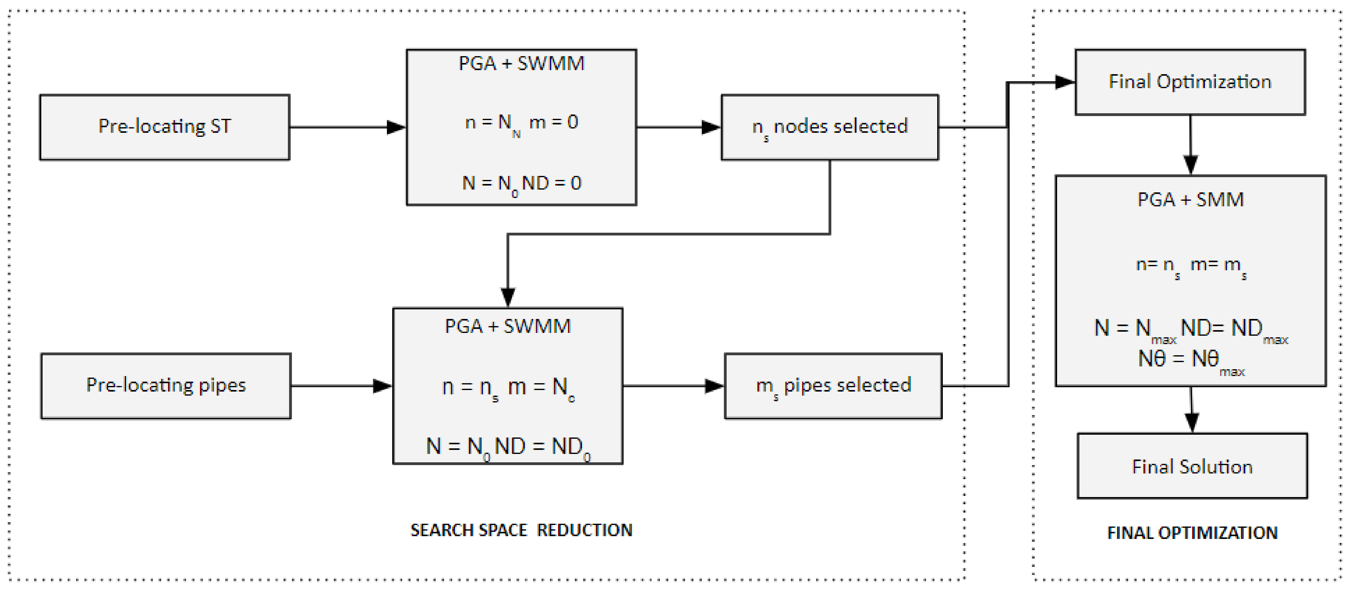
To improve the efficiency of the model, an SSR method similar to that proposed by Ngamalieu-Nengoue et al. [20] has been used. This method aims to decrease the calculation time in drainage network rehabilitation models through an interactive process that decreases the SS with the use of a PGA. Specifically, the methodology consists of two stages that are summarized in Figure 4.

As a first stage, the methodology focuses on determining the probable location of the STs. For this, a series of simulations (N_it) are carried out with the optimization model considering all the nodes of the network as possible ST locations and without considering the change of pipes (n = N_N; m = 0). Regarding the discretization of the cross-section, a reduced range N = N₀ is used. This simplification is valid because the objective is to pre-locate the ST and not to reach an optimization of the ST dimension. The simulations obtained are classified according to the values that the objective function yields. Then, a percentage of the best solutions found (p_n) are selected. An analysis of the genomes obtained is performed from this selected group, determining the number of n_s nodes in which it is highly probable that an ST is located.

In the second stage, the goal is to locate the pipes that likely require a pipe change. To achieve this, a new set of N_it simulations is run. In this process, the nodes considered are those obtained in the previous stage (n = n_s). As for the pipes, they are considered as candidates to change all the pipes in the network (m = N_c). The range of pipes used as decision variable is a reduced range as is the ST cross-section discretization (ND = ND₀; N = N₀). After the simulations, a classification of the best solutions obtained is made according to the values of the objective function. A percentage of the best solutions p_n is selected, and an analysis of the genomes obtained is carried out to finally determine the number of candidate pipes to be renewed (m = m_s). The SSR procedure has been studied previously, giving good results [20]. Its use was deepened in later studies [30], in which the authors showed the results of applying this method in different ways; their results show the suitability of implementing an SSR method in this type of problem.

Once the SS for solutions has been reduced, a final network optimization is carried out, that is, locating and dimensioning the ST, the pipes to be renewed and the hydraulic controls. Regarding hydraulic controls, since their installation is linked to the installation of an ST, they are not considered in the SS reduction process. In the final optimization, although the number of decision variables has been reduced, each of these variables must explored be more in-depth. Consequently, the discretization of the ST cross-section takes a full range (N = N_max). Likewise, the range of candidate diameters for the pipes will also be a full range (ND = ND_max). The opening degrees of the hydraulic control will be defined as Nθ. With these determined parameters, a final simulation is carried out in which the best solution of the process is obtained.

In summary, the optimization process is made up of two parts. In the first part, the decision variables are reduced by locating the probable ST locations and conduits to renew. The level of detail of each of the variables is small but valid for the established objectives. In the second part, a final optimization was carried out where the location and final dimensions of ST, pipes and hydraulic controls were determined. A smaller number of variables were used in this part, but with a higher level of detail.

4. Case Study

4.1. Description of the Network

The proposed methodology was tested for various drainage networks. In order to show its application, E-Chico network located in Bogotá (Colombia) was selected as a case study (Figure 5). This network covers an area of 51 hectares and limits with the Andes in its East end. The difference in elevation between the highest and lowest points is 39 m in height. Figure 6 shows a digital elevation model of the area. In this figure, it is easy to realize the role that the hills play in the network. Near the hills, the slope of the terrain is very steep. The slopes of the network pipes vary from 7.22% as maximum value (near the Andes) to 0.16% as minimum value, close to the outlet. The area is divided into 35 hydrological sub-basins. The network has a total length of 5000 m. Pipes’ diameters have values from 300 mm to 1400 mm. Further details of this network were presented in the work of Ngamalieu-Nengoue et al. [26], and its use allows comparison of results. Data used for the case study is attached to this article as Supplementary Materials.

For the evaluation of the problem, a design storm was used (Figure 7), calculated by the alternate blocks method with 5 min intervals and previously defined by Ngamalieu-Nengoue et al. [26]. This design storm was calculated from an IDF curve for a return period of 10 years and a duration of 55 min. To avoid extremely high intensities, the intensity was limited to a maximum intensity of 118 mm/h corresponding to a duration of 10 min. The urban basin generates a runoff volume of 20,123 m³ and presents the nodes of the network flooded with a flood volume of 3834 m³, which is 19.07% of the runoff volume.

The network in the actual conditions and considering the design storm previously presented for the hydraulic analysis presents flooding problems in many nodes of the network, so it needs to be rehabilitated to recover its benefits and provide the security that cities require.

Table 1. Flood on nodes and cost of damage in the current state of the network.

Node	Flood Volume (m3)	Flood Area (m2)	y (m)	Cost (€)
N02	123.56	1240	0.100	135,857.00
N04	132.56	930	0.413	181,375.00
N06	501.79	1890	0.265	875,502.00
N07	23.95	1250	0.019	6644.00
N09	1.82	1130	0.002	45.00
N10	385.12	700	0.550	646,838.00
N11	25.83	820	0.032	11,288.00
N23	949.54	450	2.110	569,922.00
N32	36.65	1500	0.024	12,727.00
N33	469.82	3030	0.155	671,908.00
N34	1181.87	3270	0.361	2,131,929.00
TOTAL				5,244,035.00

shows the nodes with flooding problems and the cost of the damages caused by these floods.

The coefficients used in the cost functions of the installation of the different elements (pipes, tanks and controls) are shown in

Table 2. Coefficients of the cost terms of Pipes, STs and Hydraulic Control.

Renovation of Pipes		Installation of STs			Installation of Hydraulic Control
α	β	Cmin	Cvar	ω	γ	μ
40.69	208.06	169.23	318.4	0.65	4173.70	−210.82

. These coefficients are used with Equations (5)–(7). The cost of floods was obtained using Equation (8) using the parameters shown in

Table 3. Coefficients of flood damage cost function.

λ	r	ymax	Cmax
4.89	2.00	1.40	1268.09

.

For the optimization process, the probability of success was fixed to P_e = 80%. Finally, for every step, one hundred simulations were performed, that is, N_it = 100.

4.2. Application of the Methodology

4.2.1. Reduction of the Space of Solutions Process (SSR).

In their work, Ngamalieu-Nengoue et al. [26] discretized the ST area in a wide range of N_max = 40. In addition, the 25 different diameters were available for the rehabilitation of pipes. Finally, the losses in the hydraulic controls are a continuous variable and need to be discretized as well. The valve travel was divided into 10 fractions on a logarithmic scale. Moreover, an additional value of 0 was used to describe ST where hydraulic control was not needed. The head loss coefficient was calculated using Equation (2). With these data, the size of the problem was calculated using Equation (12), giving a problem size of 2.2·10¹¹⁷. This constitutes a very big problem that needs to be reduced.

The first stage of the SSR process is the pre-location of STs. The parameters defined to carry out this process are n = N_N = 35 (that is, all the nodes are considered the pre-location process of ST) and N = N₀ = 10 (the discretization of the ST area reduced to this value). In this process, the renewal of pipes is not considered (m = 0).

With these defined parameters, the N_it simulations are carried out. From these simulations, a percentage of the best solutions p_n = 5% is selected. In each of the simulations of the selected percentage, the nodes where ST has been installed are analyzed, generating a list of nodes where an ST is possibly installed.

The second stage of the SSR process considers the previously selected nodes n = ns. The discretization of the ST is kept in a narrow range (N = N₀ = 10). In this stage, it is considered that all the pipes in the network can be candidates to be replaced (m = NC), and the range of diameters that pipes can take is reduced (ND = ND₀ = 10).

Table 4. Reduced range of diameters.

Diameter (mm)

300

400

600

800

1000

1200

1500

1800

2000

shows the values of the nine diameters considered in this reduced range. The option of not changing the diameter of the pipe is also considered if its capacity is sufficient. An additional restriction is to prevent one of the pipes from being replaced by another of smaller diameter.

The PGA parameters are the same defined for stage one P_e = 80%, N_it = 100. Once the N_it simulations have been carried out, a percentage of the best solutions is selected (p_n = 5%). From this selected percentage, the pipes that have been changed are analyzed and a list of probable pipes that must be renewed is generated. After the SSR process, the size of the problem was reduced to SS = 3.6·10⁸². Figure 8 shows the preselected nodes and pipes in the SSR process.

4.2.2. Final Optimization

For the final optimization, the previously located nodes and pipes n = n_s, m = m_s are considered, but in this stage, the discretization of the ST area takes a wide range: N = N_max = 40. In the same way, pipe diameter values are selected from the full range of available diameters (

Table 5. Complete range of diameters (mm).

Diameters (mm)
300	350	400	450	500	600	700	800	900	1000	1100	1200
1300	1400	1500	1600	1800	1900	2000	2200	2400	2600	2800	3000

). Thus, the range of variation of these decision variables is ND = ND_max = 25.

This stage also includes the option of installing hydraulic controls at the outlet of the STs. The discretization of the opening range of the gate valve is Nθ = Nθ_max = 10. With all these values (n, m, N, ND and Nθ), an optimization is carried out that generates the final solution of the process.

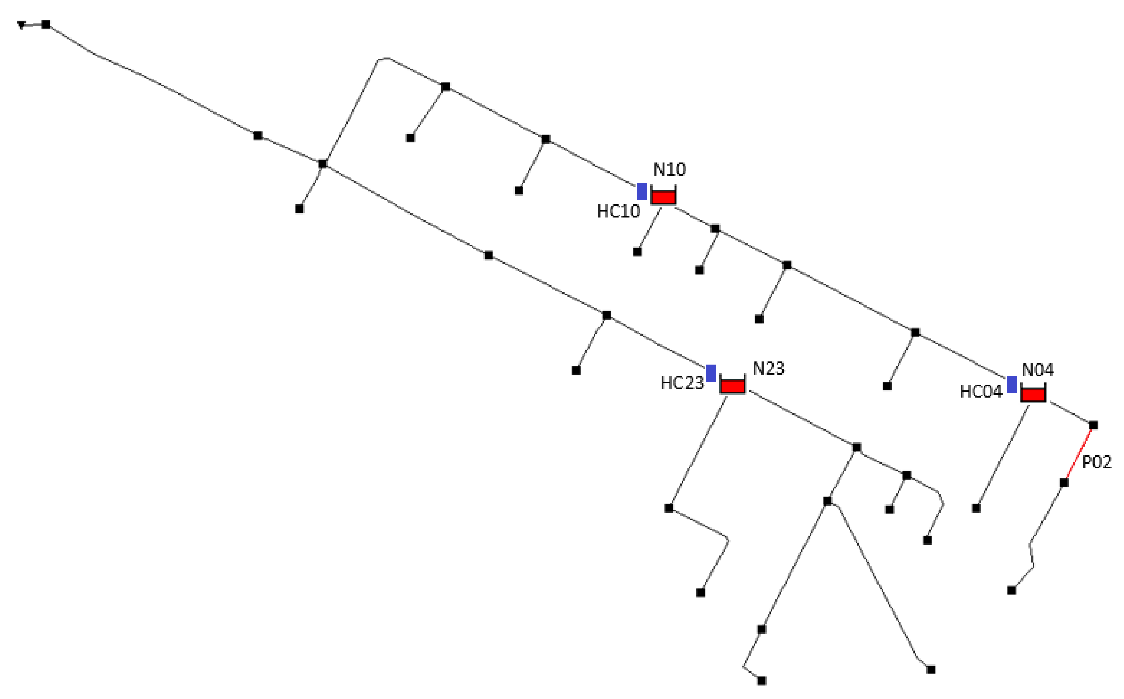
5. Results

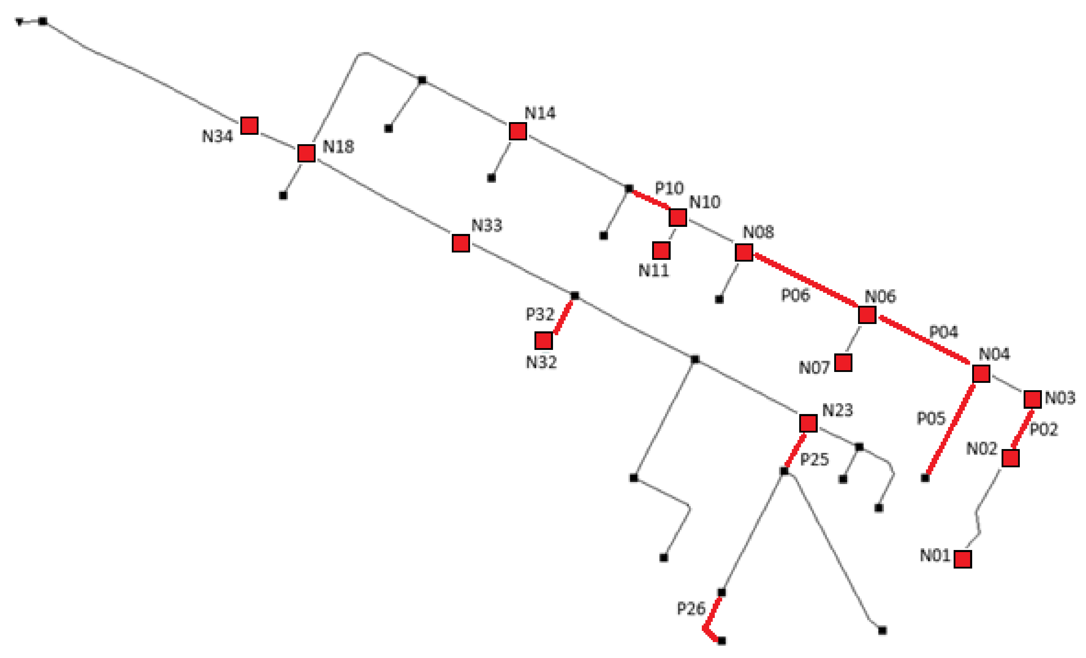
The results of the final optimization are as follows. It is required to replace the current P02 pipe with a diameter of 400 mm with another with a diameter of 500 mm. Three STs must be installed in the nodes N04, N10 and N23.

Table 6. Area and volume required in STs.

Node	Area (m2)	Volume (m3)
N04	550.00	946.00
N10	1050.00	2299.50
N23	1050.00	274.50

shows the required volume of the STs. Finally, it is required to install three hydraulic control elements must be installed in pipes P04, P10 and P23. The local head loss that these elements must generate is detailed in

Table 7. Loss coefficient k required in hydraulics control elements.

ID	Location	k	θ
HC04	P04	14.73	18.93%
HC10	P10	6.64	26.41%
HC23	P23	161.01	6.97%

. Figure 9 shows the elements to be installed and their location. With these actions, the objective function has a value of 203,859.69 € made up of the following terms: cost of pipe renovation 6583.81 €, cost of installation of STs 181,540.69 €, cost of installation of hydraulic control elements 7671.75 € and the cost of flood damages 12,701.00 €.

These results considerably improve those obtained by Ngamalieu-Nengoue et al. [21]. Table 8 compares the rehabilitation costs of different methodologies:

Case (a). Ngamalieu-Nengoue et al. method, changing only pipe diameters.

Case (b). Ngamalieu-Nengoue et al. method, only installing STs.

Case (c). Ngamalieu-Nengoue et al. method, combining both options.

Case (d). Proposed methodology, including the SSR and the use of hydraulic controls.

Table 8. Comparison of the objective functions.

Methodology	Problem Size (SS)	Terms of the Objective Function
		Pipe Cost	ST Cost	Hydraulic Control Cost	Flood Damage Cost	Total
Case (a)	4.0·× 1038	766,761.00 €	0.00 €	-	24,753.00 €	791,214.00 €
Case (b)	5.8·× 1061	-	268,063.00 €	-	5392.00 €	273,455.00 €
Case (c)	4.2·× 1069	14,927.00 €	186,353.00 €	-	12,701.00 €	213,981.00 €
Case (d)	3.6·× 1082	6583.81 €	181,540.69 €	7671.75 €	8063.44 €	203,859.69 €

Table 8. Comparison of the objective functions.

Methodology	Problem Size (SS)	Terms of the Objective Function
		Pipe Cost	ST Cost	Hydraulic Control Cost	Flood Damage Cost	Total
Case (a)	4.0·× 1038	766,761.00 €	0.00 €	-	24,753.00 €	791,214.00 €
Case (b)	5.8·× 1061	-	268,063.00 €	-	5392.00 €	273,455.00 €
Case (c)	4.2·× 1069	14,927.00 €	186,353.00 €	-	12,701.00 €	213,981.00 €
Case (d)	3.6·× 1082	6583.81 €	181,540.69 €	7671.75 €	8063.44 €	203,859.69 €

There is an improvement both in the total value of the objective function and in the value of flood damage. The results indicate that when implementing a hydraulic control element, a slowdown of the water flow is generated. This reduction of the flow downwards induces the system to use the volume of the network more efficiently, reducing both the costs of the rehabilitation of the network and flood levels. In other words, the introduction of hydraulic control allows finding better solutions for the rehabilitation of drainage networks.

It is important to highlight that the inclusion of hydraulic controls allows reducing the cost in every term. That is, in comparison with previous results, pipe cost, ST cost and flood damage cost using the proposed methodology are reduced with respect to the works by Ngamalieu-Nengoue et al. [21].

Including hydraulic controls increase the size of the problem. This might be the main drawback of the methodology. However, this problem was solved using an SSR process that reduced considerably the problem.

6. Conclusions

Extreme rains and impermeable ground due to population growth have caused many cities to experience flooding. Drainage networks were not designed for these new conditions, so adaptation is necessary. Implementing tanks to retain flow peaks is a well-studied alternative that has proven to have advantages over other methods in extreme rain events. In the literature, there are many techniques to rehabilitate drainage networks and reduce damage caused by floods. However, none of them were based on hydraulic simulation and considered at the same time the replacement of pipes, the installation of STs and the introduction of hydraulic control.

One of the main contributions of this work is the inclusion of hydraulic control as a complementary rehabilitation strategy to the replacement of pipes and the STs installation. For this, it has been necessary to represent in economic terms all the parameters involved in the process, including investment costs and costs associated with flood damage. In this sense, another contribution has been the inclusion of hydraulic control and its valuation in economic terms. The participation of hydraulic control has been possible to make it compatible with the part of the objective function previously defined. This formulation of the objective functions in monetary units is very useful for decision-makers in the development of a rehabilitation project.

The proposed method also includes improvements in the solution space exploration capabilities. In this way, the SSR methodology has been generalized to be compatible with the presence of potential hydraulic control devices. Likewise, the specific convergence criterion G_max of the optimization model has been formulated explicitly in terms of the probability of success.

The applicability of the method has been shown through the case study presented. Given that the study network is located in Colombia, the prices used as a reference have been those of that country, although the numerical values have been translated into Euros to facilitate understanding. As can be seen, the application of the proposed methodology, which includes hydraulic control, leads to solutions for the rehabilitation of the drainage networks that are cheaper and with lower flood costs. In summary, implementing hydraulic controls reduces flood levels and the size of the necessary structures. Therefore, we can achieve the conclusion that hydraulics controls are valid and effective elements in the rehabilitation of drainage networks.

One of the main limitations of the method, derived from the initial working hypotheses, is the impossibility of modifying the topology of the network. This means that it is not possible to add new pipes. Indirectly, this means that all the STs added to the network must be installed in on-line mode. Undoubtedly, one of the improvements of this work lies in allowing the installation of off-line STs with new pipes that connect these tanks to the network and included in the methodology the determination of the devices that must be activated for the filling and emptying these tanks. In any case, obtaining this improvement is something that seems a natural consequence of the results obtained in this work.

Finally, the results obtained comprise a feasible solution for a defined problem with a defined rainfall. Depending on this rainfall, different solutions will be obtained. Hence, there is no optimal solution, and any problem must be solved in accordance with budget availability, design criteria, etc. This an open field for future investigations.