Simulation of Pollution Load at Basin Scale Based on LSTM-BP Spatiotemporal Combination Model

Abstract

Accurate simulation of pollution load at basin scale is very important for controlling pollution. Although data-driven models are increasingly popular in water environment studies, they are not extensively utilized in the simulation of pollution load at basin scale. In this paper, we developed a data-driven model based on Long-Short Term Memory (LSTM)-Back Propagation (BP) spatiotemporal combination. The model comprises several time simulators based on LSTM and a spatial combiner based on BP. The time series of the daily pollution load in the Zhouhe River basin during the period from 2006 to 2017 were simulated using the developed model, the BP model, the LSTM model and the Soil and Water Assessment Tool (SWAT) model, independently. Results showed that the spatial correlation (i.e., Pearson’s correlation coefficient is larger than 0.5) supports using a single model to simulate the pollution load at all sub-basins, rather than using independent models for each sub-basin. Comparison of the LSTM-BP spatiotemporal combination model with the BP, LSTM and SWAT models showed that the performance of the LSTM model is better than that of the BP model and the LSTM model can obtain comparable performance with the SWAT model in most cases, whereas the performance of the LSTM-BP spatiotemporal combination model is much better than that of the LSTM and SWAT models. Although the variation of the simulated pollution load with the LSTM-BP model is high under different hydrological periods and precipitation intensities, the LSTM-BP model can track the temporal variation trend of pollution load accurately (i.e., the RMSE is 6.27, NSE is 0.86 and BIAS is 19.46 for the NH₃ load and the RMSE is 20.27, NSE is 0.71 and BIAS 36.87 is for the TN load). The results of this study demonstrate the applicability of data-driven models, especially the LSTM-BP model, in the simulation of pollution load at basin scale.

1. Introduction

Accurate simulation of pollution load at basin scale is very important for controlling pollution. At present, the estimation of pollution load in a basin is mainly performed using physical models, such as the Hydrological Simulation Program-Fortran (HSPF) model [1,2,3], the Soil and Water Assessment Tool (SWAT) model [4,5,6] and the Agricultural Non-Point Source (AGNPS) model [7,8,9]. However, these models describe the hydrological process and the transport processes of pollutants with complex physical mechanisms. Thus, these models are usually sensitive to parameters, data and resolution [10]. Moreover, they require great effort in terms of model calibration because of the uncertainty in model structure and parameter estimation [11].

Data-driven models can learn complex associations between inputs and outputs instantly and work with high accuracy even without prior knowledge of the underlying processes [12]. However, despite their advantages, the application of data-driven models in simulating pollution load at basin scale is still scarce. Several data-driven models, such as the Support Vector Machine (SVM) model [13], the Auto-Regressive Moving Average (ARMA) model [14] and the Back Propagation Neural Network (BPNN) model [15], have been applied in different domains of water environment modeling. These conventional machine-learning models achieved similar or even better performance compared with the physical- or process-based models in many cases, including the water quality simulation [15], the soil water and groundwater simulation [16,17] and the runoff simulation [18]. However, conventional machine-learning models are not specifically designed for processing temporal data and cannot retain temporal information, which is important in the case of time-series problems [19].

Compared with conventional machine-learning models, deep-learning models, such as the Recurrent Neural Network (RNN) model [19] and the Long-Short Term Memory Neural Network (LSTMNN) model [20], are characterized by high dimensionality, nonlinearity, self-adaptability and extensive inter-connectivity among neurons [21]. The RNN model solves the problem of conventional machine-learning models not being able to retain temporal information by establishing weight connection between neurons [19]. However, the RNN model is not problem-free. The primary challenge to RNN is exploding and vanishing gradient problem [22]. The LSTM model, by adding gate functions to its memory unit, overcomes the issues encountered by RNN, as well as preserving the long-term temporal information of the time-series data [23]. Due to the unique network structure, the LSTM model is more suitable for simulating hydrological events with long time series [24]. In addition, Kratzert et al. [25] trained LSTM models to simulate the rainfall-runoff process for hundreds of basins over the U.S. Results demonstrated that the performance of the LSTM model in rainfall-runoff simulation is better than that of the hydrological model in most basins. All aforementioned studies have presented the potential of LSTM in water environment modeling applications but they have not been utilized in the simulation of pollution load at basin scale. The models similar to that of Kratzert et al. [25] only use data from their own sub-basin as input, neglecting the fact that the associated input from nearby sub-basins may improve simulation performance. Furthermore, the studies mostly take time-series data (i.e., meteorology, precipitation intensity, runoff, month and hydrological period) as the input, neglecting the effects of spatial data (i.e., digital elevation, soil type and land use). Although the simulation with only time-series data can achieve desirable results in some cases, whether it can be further improved in model performance with spatial data as input is still vague.

The objectives of this study are to develop a data-driven model based on LSTM-BP spatiotemporal combination for the simulation of pollution load and to evaluate the model’s simulation performance. The model comprises several time simulators based on LSTM and a spatial combiner based on BP. First, the spatial correlation between the pollution load at different sub-basins is calculated by Pearson’s correlation coefficient. Then, the LSTM-BP model is compared with the BP, LSTM and SWAT models to evaluate the applicability of the LSTM-BP model in simulating pollution load at basin scale. Finally, the LSTM-BP model’s simulation performance is analyzed under different hydrological periods and precipitation intensities.

2. Materials and Methods

2.1. Study Area

The Zhouhe River is the largest tributary on the left bank of the Qujiang River in northeastern Sichuan province, China (30°00′ to 32°45′ N, 106°17′ to 109°00′ E) with an area of 11,180 km² and elevation ranging from 188 to 2669 m (Figure 1). The average annual flow is 22 m³/s.

2.2. Data Acquisition

2.2.1. Time-Series Data

Meteorological data, including precipitation, minimum and maximum temperatures, relative humidity, wind speed and solar radiation, were monitored at weather stations in the Zhouhe River basin (Figure 1a). Flow rates (i.e., runoff) and concentrations of NH₃ and TN were measured at the automatic water quantity monitoring stations at the outlet of the basin (i.e., Liangtan station, shown in Figure 1a). Pollution discharged from point sources, including industrial and urban sewage and atmospheric deposition, were monitored by the Sichuan Environmental Monitoring Center. The time range is from 1 January 2006 to 31 December 2017 and the monitoring frequency is days, as well as these time series data were measured in accordance with China’s Surface Water Quality Measurement Code.

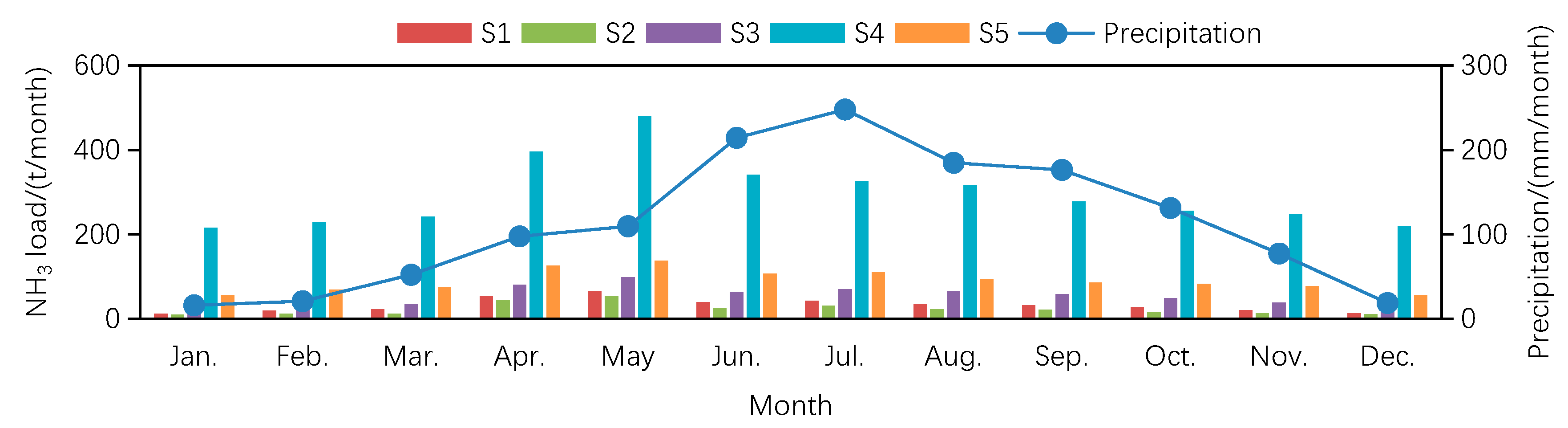
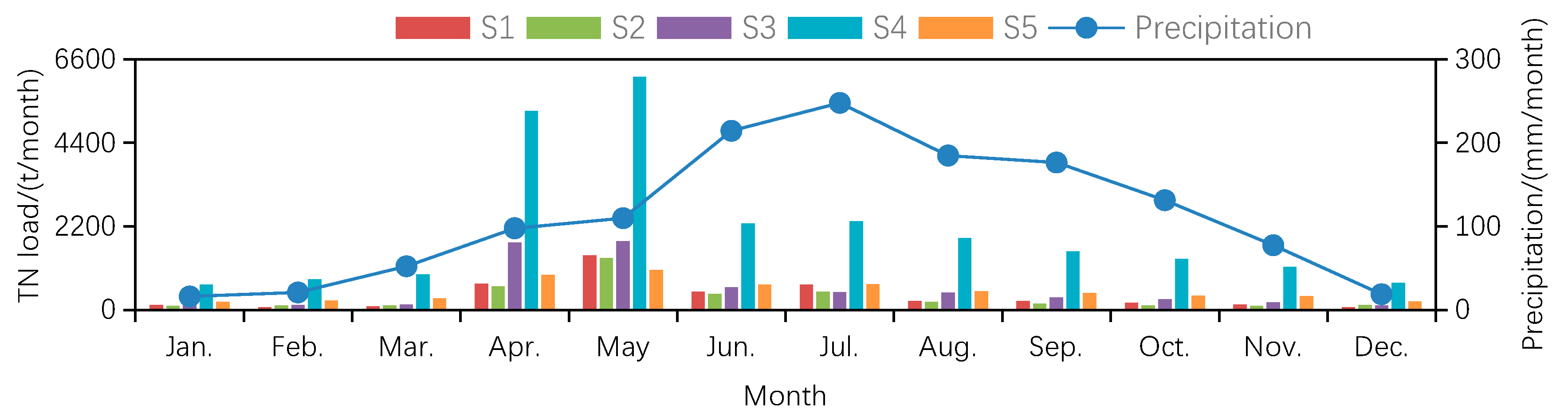
The values of monthly NH₃ load, TN load and precipitation on the validation set are shown in Figure 2 and Figure 3, respectively. Since the impact of precipitation on runoff and pollution load in the basin is different under different precipitation intensities and precipitation intensity influences the amount of water that dilutes the pollutants, the precipitation was divided into six levels, including no rain, light rain (precipitation between 0 and 10 mm, inclusive), moderate rain (precipitation between 10 and 25 mm, inclusive), heavy rain (precipitation between 25 and 50 mm, inclusive), torrential rain (precipitation between 50 and 100 mm, inclusive) and severe torrential rain (precipitation greater than 100 mm). Moreover, pollution load shows significant differences in different months and hydrological periods [26] and these differences play a crucial role in achieving an accurate simulation. According to the total precipitation of each month, it was divided into flood season, dry season and flat season. In the Zhouhe River basin, the annual precipitation is concentrated in the flood season (during the period from June to October). The dry season is from December to March of the following year. There is less precipitation during the dry season and the pollution load is significantly reduced due to the reduced runoff. The flat season is from April to May and November. During the flat season, the pollutants accumulated on the soil surface during the dry season converge into the rivers through surface runoff due to the increase of air temperature and precipitation. The flow rates and pollutants concentrations varied in the dry, flat and flood seasons.

2.2.2. Spatial Data

The Digital Elevation Model (DEM) used the global land GTOPO30 data from the United States Geological Survey (USGS)-Earth Resources Observation and Science (EROS) data center. Land use information for 2018 was obtained from the Chinese Academy of Sciences (Figure 1b). According to the World Reference Base [27], the soil in the calculation area includes 11 types (Figure 1c). Soil physical properties (i.e., particle size distribution, bulk density, field capacity and hydraulic conductivity) were obtained from the soil database and field survey in the Zhouhe River basin. Soil nutrient (i.e., TN content) was obtained from local soil survey reports (Figure 1d). The basin was divided into five sub-basins (i.e., S1 to S5 as shown in Figure 1a). Basic information of the five sub-basins (S1–S5) is show in

Table 1. Basic information of the five sub-basins (S1–S5).

Sub-Basin		S1	S2	S3	S4	S5
Area (km2)		2040.1	816.0	2448.2	3019.4	2856.2
Mean slope (degree)		12.2	8.4	16.8	13.5	11.4
Drainage density (km−1)		0.174	0.201	0.165	0.164	0.157
Soil properties	Clay (%)	21.56 ± 4.87 *	22.74 ± 8.48	16.24 ± 5.80	19.04 ± 6.99	17.94 ± 10.27
	Silt (%)	35.78 ± 12.04	31.18 ± 12.87	40.04 ± 18.12	30.17 ± 11.38	22.17 ± 15.84
	Sand (%)	41.16 ± 14.55	40.09 ± 19.72	44.26 ± 15.10	49.51 ± 15.07	59. 51 ± 18.40
	Hydraulic conductivity (10−6 m·s−1)	13.46 ± 8.71	12.41 ± 6.17	9.77 ± 8.54	10.24 ± 6.60	16.51 ± 8.31
	Bulk density (g cm−³)	1.38 ± 0.56	1.36 ± 0.44	1.37 ± 0.61	1.36 ± 0.52	1.33 ± 0.32

* Mean and STD stand for the mean value and the deviation.

.

2.3. Data Preprocessing

To avoid data dependence on measurement units and to improve the convergence speed of the calibration, data normalization was conducted before entering the model [28]. The data (i.e., pollution load, meteorology, runoff, digital elevation, land use and soil type data) were normalized between 0 and 1 by linear normalization. The normalization formula is as follows:

$$x^{*}=\frac{x-mi{n}_x}{ma{x}_x-mi{n}_x},$$

(1)

where x is the original data and min_x and max_x represent the minimum and maximum values of the variable of the original data x, respectively. The normalized value of pollution load simulated by the model was converted to the output layer’s actual value by the following formula:

$$x=x^{*}\left(ma{x}_x-mi{n}_x\right)+mi{n}_x.$$

(2)

For nominal features such as month, hydrological period and precipitation intensity that do not have sequence and cannot be compared in size, simple values could not be used instead, because the attribute value of such features affects the operation of the model weight matrix. One-hot encoding is used to convert these nominal features into binary codes [29]. For example, one-hot encoding of the hydrological period features included “001,” “010” and “100” for the flood season, the dry season and the flat season, respectively.

2.4. Spatial Correlation Analysis

The basin was divided into five sub-basins (Figure 1a). More information about the five sub-basins is shown in Table 1. Pearson’s correlation coefficient was used to measure the correlation between two random variables:

$${\mathrm{R}}^2\left(x_i,x_j\right)=\frac{Cov\left(x_i,x_j\right)}{\sigma \left(x_i\right)\sigma \left(x_j\right)},$$

(3)

where x_i and x_j respectively represent the series of NH₃ or TN load at sub-basin i and sub-basin j; $Cov(·)$ is covariance and $\sigma (·)$ is standard deviation. The correlations in the pollution load at the sub-basins are shown in

Table 2. Spatial correlation between the pollution load at different sub-basins.

R2	S1		S2		S3		S4		S5
	NH3	TN	NH3	TN	NH3	TN	NH3	TN	NH3	TN
S1	1.00	1.00	0.74	0.71	0.76	0.67	0.81	0.72	0.32	0.33
S2	0.74	0.71	1.00	1.00	0.54	0.51	0.68	0.64	0.27	0.27
S3	0.76	0.67	0.54	0.51	1.00	1.00	0.97	0.97	0.48	0.46
S4	0.81	0.72	0.68	0.64	0.97	0.97	1.00	1.00	0.75	0.87
S5	0.32	0.33	0.27	0.27	0.48	0.46	0.75	0.87	1.00	1.00

. Notably, except the correlation coefficients between S1 and S5, between S2 and S5 and between S3 and S5 which are small due to the long distance and no confluence between the two sub-basins, the correlation coefficient in the pollution load between sub-basins is larger than 0.5. The strong spatial correlation supports using a single model to simulate the pollution load at all sub-basins, rather than using independent models for each sub-basin, because the associated inputs from nearby sub-basins can improve simulation accuracy [22].

2.5. LSTM-BP Model Setup

2.5.1. LSTM-Based Temporal Simulator

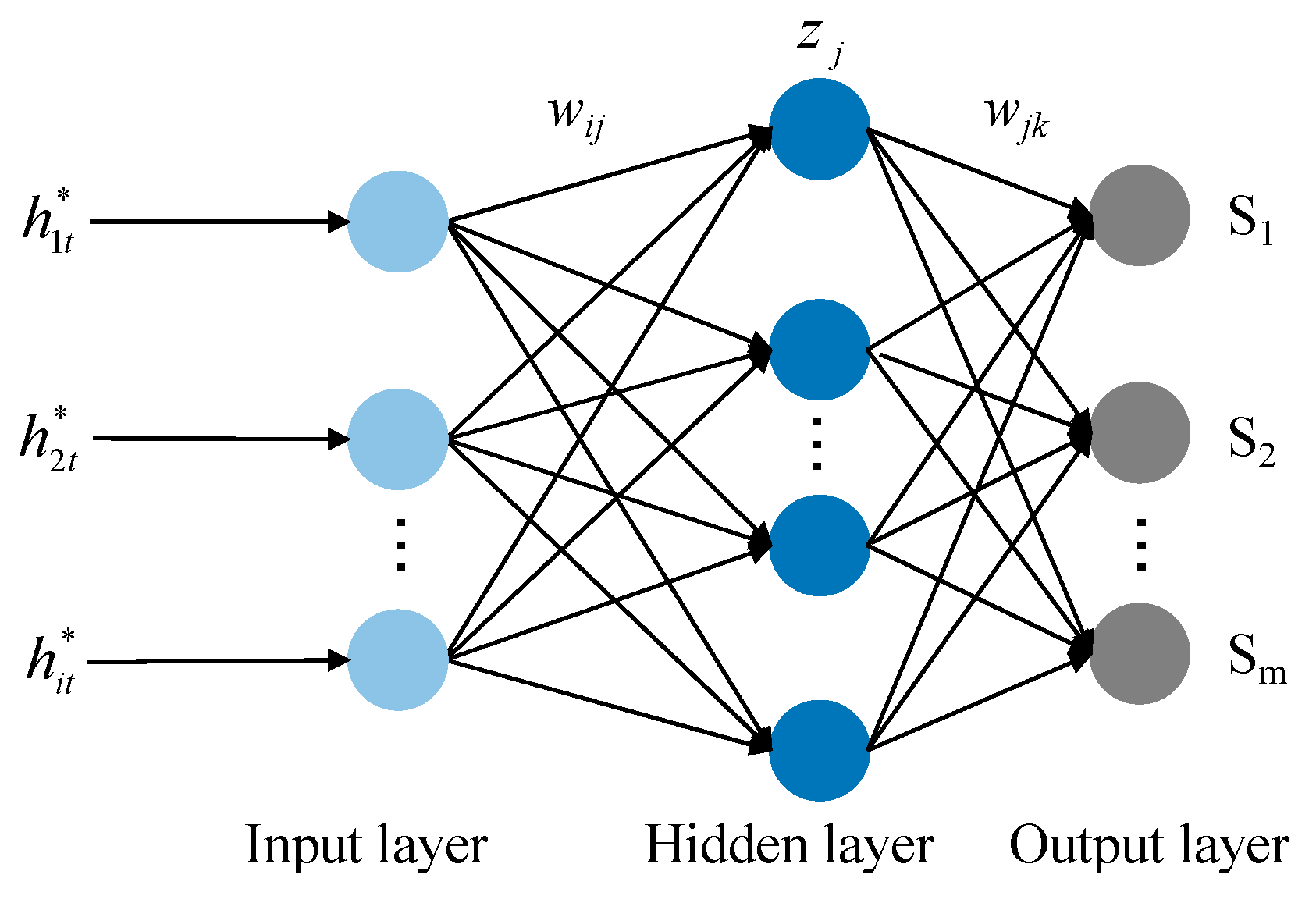
Using the excellent ability of the LSTM model to remember long-term dependencies in time-series forecasting and modeling problems [30], a time simulator based on LSTM was established for each sub-basin to extract the time-series features of historical data and the complicated nonlinear relationships between input features automatically (Figure 4). For the LSTM model, at sub-basin i, the input layer is an input vector (x_t, x_t−1, …, x_t−n) and x_t includes meteorology, precipitation intensity, runoff, month, hydrological period and pollution load. The hidden layer is the output (i.e., pollution load simulated value $h_{it}$ at time t). At time t, the input of the LSTM memory unit includes the current moment input variable $x_t$, the previous moment hidden layer state variable $h_{t-1}$ and the previous moment memory unit state variable $c_{t-1}$. The model passes through the forgotten gate $f_t$, the input gate $i_t$ and the output gate $o_t$ in turn. The output of LSTM memory unit includes the current moment output variable $h_t$ and the current moment memory unit state variable $c_t$. The calculation formulas are as follows:

$$f_t=\sigma \left(W_f\left[h_{t-1},x_t\right]+b_f\right),$$

(4)

$$i_t=\sigma \left(W_i\left[h_{t-1},x_t\right]+b_i\right),$$

(5)

$${\tilde{c}}_t=\tan \mathrm{h}\left(W_c\left[h_{t-1},x_t\right]+b_c\right),$$

(6)

$$c_t=f_t·c_{t-1}+i_t·{\tilde{c}}_t,$$

(7)

$$o_t=\sigma \left(W_o\left[h_{t-1},x_t\right]+b_o\right),$$

(8)

$$h_t=o_t·\tan \mathrm{h}\left(c_t\right),$$

(9)

$$y_t=W_d·h_t+b_d,$$

(10)

where $W_f$, $W_i$, $W_c$, $W_o$, $W_d$, $b_f$, $b_i$, $b_c$, $b_o$ and $b_d$. are adjustable parameter matrices or vectors (these parameters were automatically optimized by the reverse error propagation algorithm in the calibration), $\mathsf{\sigma }$ is the Sigmoid activation function and tanh is the hyperbolic tangent activation function. In the simulation of pollution load, the input gate controls the influence of the new measured value on the current simulated value, while the output gate controls the influence of a past trend. For example, when the pollution load changes slowly, the output gate tends to close, retaining the trend information; when the pollution load changes sharply, the input gate is opened to obtain new observations.

2.5.2. BP-Based Spatial Combinatory

Using the nonlinear expression ability of the BP model [31], a spatial combiner based on BP was constructed to describe the spatial relationships among the sub-basins automatically, thus achieving the accurate simulation of pollution load at each sub-basin (Figure 5). The output $z_j$ of the jth neuron in the hidden layer of the BP neural network is as follows:

$$z_j=f\left({\sum }_{i=1}^m{w}_{ij}{h}_{it}^{*}+b_j\right).$$

(11)

The $z_j$ after the hidden layer mapping of BP neural network is directly used as the input of the BP model’s output layer and the output layer performs nonlinear fitting. The output $S_k$ at sub-basin k in the output layer is as follows:

$$S_k={\sum }_{j=1}^n{w}_{jk}{z}_j+b_k,$$

(12)

where $h_{it}^{*}$ is a vector composed of the underlying surface characteristics (i.e., digital elevation, land use and soil type) of sub-basin i and the output $h_{it}$ of the LSTM model at time t; w_ij, w_jk, b_j and b_k are adjustable parameter matrices or vectors (these parameters will be automatically optimized by the reverse error propagation algorithm in the calibration); m is the total number of sub-basins, n is the number of neurons in the hidden layer and $f(·)$ is the activation function of neurons (Sigmoid activation function was selected in this study).

2.5.3. LSTM-BP Model

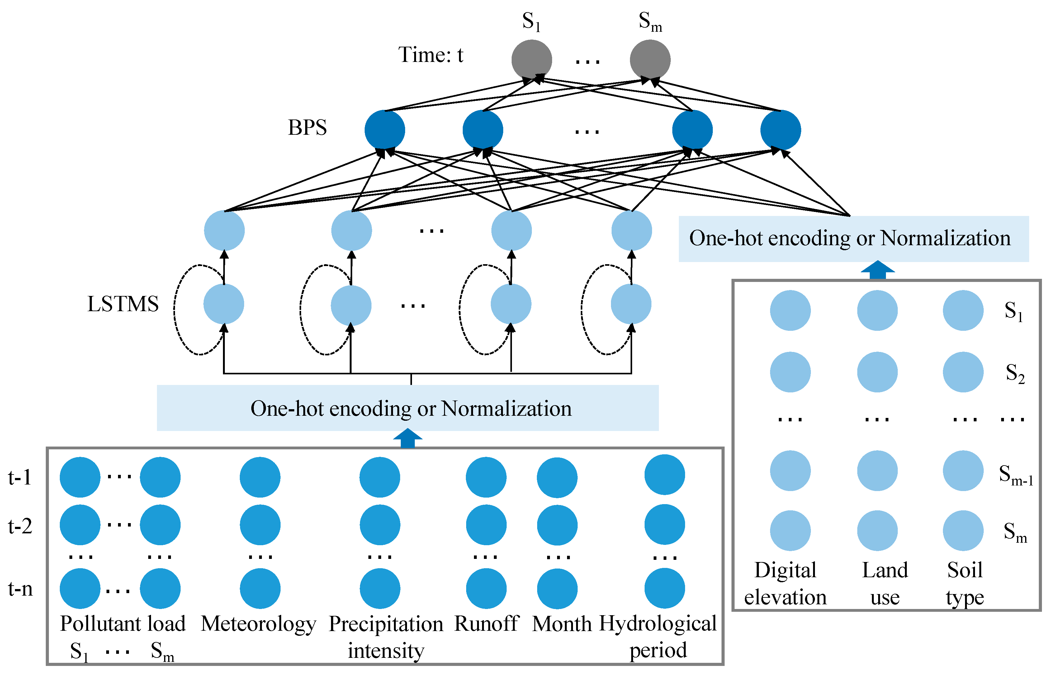
Using the deep-learning framework Keras, a LSTM-BP spatiotemporal combination model for the simulation of pollution load at basin scale was constructed (Figure 6). The model comprised several time simulators based on LSTM and a spatial combiner based on BP. Historical data of time-series of the meteorology, precipitation intensity, runoff, month, hydrological period and pollution load were selected as the LSTM model’s input. A time simulator based on LSTM was used to simulate changes of the pollution load in each sub-basin. Spatial data, including digital elevation, land use and soil type and the hidden layer output of LSTM models, were treated as the BP model’s input. Then, a BP-based spatial combiner was released to capture the spatial relationships among the sub-basins to obtain the simulated value of pollution load at each sub-basin at time t at the output layer. The calibration period is from 1 January 2006 to 31 December 2014 and the validation period is from 1 January 2015 to 31 December 2017.

2.5.4. Tuning for Hyper-Parameters

The optimal hyper-parameters were determined through multiple experiments. There were two hidden layers of the LSTM network (15 neurons in the first hidden layer and 10 neurons in the second hidden layer) and one hidden layer of the BP network (64 neurons). A dropout layer was set on the hidden layer with a dropout rate of 0.3 to reduce overfitting. The maximum number of iterations is 200. The learning rate is 0.001. The batch_size is 50. The window size is 30. Adam stochastic gradient descent algorithm is used. Root Mean Square Error (RMSE) is used as the loss function.

2.6. Contrast Model Setup

2.6.1. BP Model

The BP model (Figure 5) implemented in this study was similar to the proposed LSTM-BP model (Figure 6). A single BP model was used for all sub-basins. The BP model’s input was time-series data including meteorology, precipitation intensity, runoff, month, hydrological period and pollution load at each sub-basin and spatial data including digital elevation, land use and soil type at each sub-basin. The BP model’s output was the simulated value of pollution load at each sub-basin at time t. The BP model also contained one hidden layer (64 neurons). A dropout layer was set on the hidden layer with a dropout rate of 0.3. The maximum number of iterations is 200. The learning rate is 0.001. The batch_size is 50. Adam stochastic gradient descent algorithm is used. RMSE is used as the loss function. The calibration period is from 1 January 2006 to 31 December 2014 and the validation period is from 1 January 2015 to 31 December 2017.

2.6.2. LSTM Model

The LSTM model (Figure 4) implemented in this study was similar to the proposed LSTM-BP model (Figure 6). Independent LSTM models were used for each sub-basin. The LSTM model’s input was time-series data including meteorology, precipitation intensity, runoff, month, hydrological period and pollution load at its own sub-basin. The LSTM model’s output was the simulated value of pollution load at its own sub-basin at time t. The LSTM model also contained two hidden layers (15 neurons in the first hidden layer and 10 neurons in the second hidden layer). A dropout layer was set on the hidden layer with a dropout rate of 0.3. The maximum number of iterations is 200. The learning rate is 0.001. The batch_size is 50. The window size is 30. Adam stochastic gradient descent algorithm is used. RMSE is used as the loss function. The calibration period is from 1 January 2006 to 31 December 2014 and the validation period is from 1 January 2015 to 31 December 2017.

2.6.3. SWAT Model

The SWAT model was a physical-based distributed model for simulating hydrological and pollution load in a basin. In the SWAT model, the Zhouhe River basin was divided into 128 sub-basins based on DEM data. The sub-basin was further divided into Hydrological Response Units (HRUs) based on land use and soil properties. The SWAT model first simulated the process at the HRU level and subsequently routed at the sub-basin level. The SWAT Calibration and Uncertainty Programs (SWAT-CUP) were utilized to calibrate SWAT parameters. The Sequential Uncertainty Fitting (version 2, SUFI-2) algorithm in SWAT-CUP was selected as the calibration algorithm due to its good performance in large basins. The SWAT model ran at daily time step. The calibration period is from 1 January 2006 to 31 December 2014 and the validation period is from 1 January 2015 to 31 December 2017.

2.7. Model Evaluation Indicators

The RMSE, Nash–Sutcliffe Efficiency (NSE) and Bias Ratio (BIAS) were used to evaluate the model’s performance. The RMSE reflects the degree of difference between the measured and simulated pollution load; the NSE verifies the model’s accuracy; the BIAS judges whether there is a systematic bias between the measured and simulated pollution load. The indicators are defined as follows:

$$\mathrm{RMSE}=\sqrt{\frac{1}{n}{\sum }_{i=1}^n{\left(S_i-O_i\right)}^2},$$

(13)

$$\mathrm{NSE}=1-\frac{{\sum }_{i=1}^n{\left(S_i-O_i\right)}^2}{{\sum }_{i=1}^n{\left(O_i-\overline{O}\right)}^2},$$

(14)

$$\mathrm{BIAS}=100\frac{{\sum }_{i=1}^n\left(S_i-O_i\right)}{{\sum }_{i=1}^n{O}_i},$$

(15)

where $O_i$ and $S_i$ are the measured and simulated pollution load, respectively and n is the total number of samples. The model guide developed by Moriasi et al. [32] was used to evaluate model performance.

Very good: 0.75 < NSE ≤ 1, |BIAS| < 25
Good: 0.65 < NSE ≤ 0.75, 25 ≤ |BIAS| < 40
Satisfactory: 0.5 < NSE ≤ 0.65, 40 ≤ |BIAS| < 70
Unsatisfactory: NSE ≤ 0.5, |BIAS| ≥ 70

(16)

3. Results and Discussion

3.1. Comparison of Simulation Performance with Other Models

The evaluation indicators of the BP, LSTM, LSTM-BP and SWAT models on the validation set are shown in

Table 3. Evaluation indicators of the BP, LSTM, LSTM-BP and Soil and Water Assessment Tool (SWAT) models on the validation set.

Pollutant	Sub-Basin	BP			LSTM			LSTM-BP			SWAT
		RMSE	NSE	BIAS	RMSE	NSE	BIAS	RMSE	NSE	BIAS	RMSE	NSE	BIAS
NH3 (t/day)	S1	3.43	0.86	17.78	2.91	0.89	15.84	2.27	0.92	14.28	2.84	0.90	15.17
	S2	3.15	0.87	16.42	2.69	0.90	15.68	2.23	0.93	13.79	2.67	0.92	15.09
	S3	5.32	0.84	19.09	4.13	0.89	17.98	3.42	0.91	16.13	4.53	0.89	18.25
	S4	12.23	0.79	24.45	10.63	0.81	22.42	9.31	0.83	21.44	10.45	0.82	22.16
	S5	7.28	0.82	22.43	5.23	0.89	18.34	4.16	0.90	16.48	5.18	0.89	19.53
TN (t/day)	S1	12.45	0.81	24.17	9.43	0.85	21.26	8.91	0.86	19.87	9.76	0.85	21.95
	S2	10.59	0.79	23.94	9.15	0.86	20.43	8.72	0.86	19.29	9.36	0.86	21.58
	S3	17.45	0.75	29.64	13.66	0.78	21.83	12.24	0.81	21.23	13.82	0.79	22.47
	S4	26.67	0.69	45.32	19.06	0.73	39.57	17.25	0.74	34.32	18.57	0.73	38.62
	S5	19.52	0.74	32.37	13.76	0.79	25.77	12.74	0.80	23.83	14.98	0.79	25.13

. For the NH₃ load, the BP, LSTM, LSTM-BP and SWAT models are “very good” for all sub-basins [32]. For the TN load, the BP model is “satisfactory,” “good” or “very good” for all sub-basins [32], while the LSTM, LSTM-BP and SWAT models are “good” or “very good” for all sub-basins [32]. NH₃ enters the rivers mainly in the form of dissolved N in the surface runoff, while TN enters the rivers in the form of dissolved N, as well as solid N absorbed on the suspended mass in the surface runoff and dissolved N in the sub-surface outflow [33]. Thus, the BP, LSTM, LSTM-BP and SWAT models underestimated TN peak. All models simulated the NH₃ load better than the TN load. The LSTM-BP model had the largest NSE and lowest BIAS and RMSE, demonstrating that the performance of the LSTM-BP model is much better than that of the BP, LSTM and SWAT models. Moreover, the performance of the LSTM model is better than that of the BP model and the LSTM model can achieve comparable performance with the SWAT model in most cases. These results are in substantial agreement with those of Kratzert [25]. The study by Kratzert [25] only used data from their own sub-basin as LSTM model’s input, neglecting the fact that the associated input from nearby sub-basins may improve simulation performance, while our study effectively extracted the spatiotemporal characteristics between the various data using the LSTM-BP model.

3.2. LSTM-BP Model’s Performance under Different Hydrological Periods and Precipitation Intensities

The evaluation indicators of the LSTM-BP model in different hydrological periods on the validation set are shown in

Table 4. Evaluation indicators of the LSTM-BP model in different hydrological periods on the validation set.

Hydrological Periods		Dry Season	Flat Season	Flood Season	All Year
NH3 load (t/day)	RMSE	3.98	9.31	8.97	6.27
	NSE	0.88	0.82	0.83	0.86
	BIAS	18.14	22.94	21.12	19.46
TN load (t/day)	RMSE	13.75	32.31	28.24	20.27
	NSE	0.78	0.64	0.68	0.71
	BIAS	24.43	41.28	39.03	36.87

. Among the dry season, the flat season and the flood season, the accuracy of the LSTM-BP model was highest during the dry season. Runoff seldom occurred during the dry season due to less rainfall. The pollution load, as well as the overall fluctuation, were small. The LSTM-BP model captured complicated nonlinear relationships between various factors. With the temperature and the precipitation increased during the flat season, the pollutants which accumulated on the soil surface over a long time during the dry season converged into the rivers with runoff, the pollution load peaked and the overall fluctuation increased [34,35]. We surmised that the nitrogen fertilizer application also contributed to this increase [11]. Karlen et al. [36] reported that higher TN in water was generally found after fertilizer applications. The fertilizers in Sichuan province are usually applied in spring and contain a large amount of nitrogen. The simulation accuracy of the LSTM-BP model decreased. Although the pollution load and overall fluctuation significantly increased during the flood season, the simulation accuracy of the LSTM-BP model increased.

Although the study by Baek et al. [11] analyzed the pollutant distribution under different precipitation intensities, it did not analyze the model’s simulation performance, while our study analyzed the model’s simulation performance under different precipitation intensities. The evaluation indicators of the LSTM-BP under different precipitation intensities on the validation set are shown in

Table 5. Evaluation indicators of the LSTM-BP model under different precipitation intensities on the validation set.

Precipitation Intensity		No Rain	Light Rain	Moderate Rain	Heavy Rain	Torrential Rain	Severe Torrential Rain
NH3 load (t/day)	RMSE	1.34	3.47	6.72	10.27	15.16	23.34
	NSE	0.97	0.90	0.85	0.80	0.76	0.73
	BIAS	9.85	17.16	19.89	22.64	28.19	32.27
TN load (t/day)	RMSE	8.71	12.84	17.23	22.34	27.75	36.49
	NSE	0.84	0.80	0.75	0.74	0.69	0.63
	BIAS	20.99	22.98	29.71	31.85	37.63	45.57

. Zheng et al. [37] found through tests that the increase of rainfall intensity would increase the amount of pollutants. The greater the intensity of precipitation, the greater the coefficient of runoff production, the greater the runoff, the stronger the erosion of pollutants and soil, the stronger the capacity of pollution production and transportation of pollutants, the more pollutants carried away, the greater the degree of pollution generated, that is, the more threat to the surrounding water pollution [38]. The simulation accuracy of the LSTM-BP model decreased with the increasing of the pollution load. As the precipitation intensity was small, the pollution load tended to remain stable and fluctuates less. The pollution load and the fluctuation increased in orders of magnitude below the conditions of heavy precipitation [39]. The LSTM-BP model better simulated the stable fluctuation of the pollution load [40].

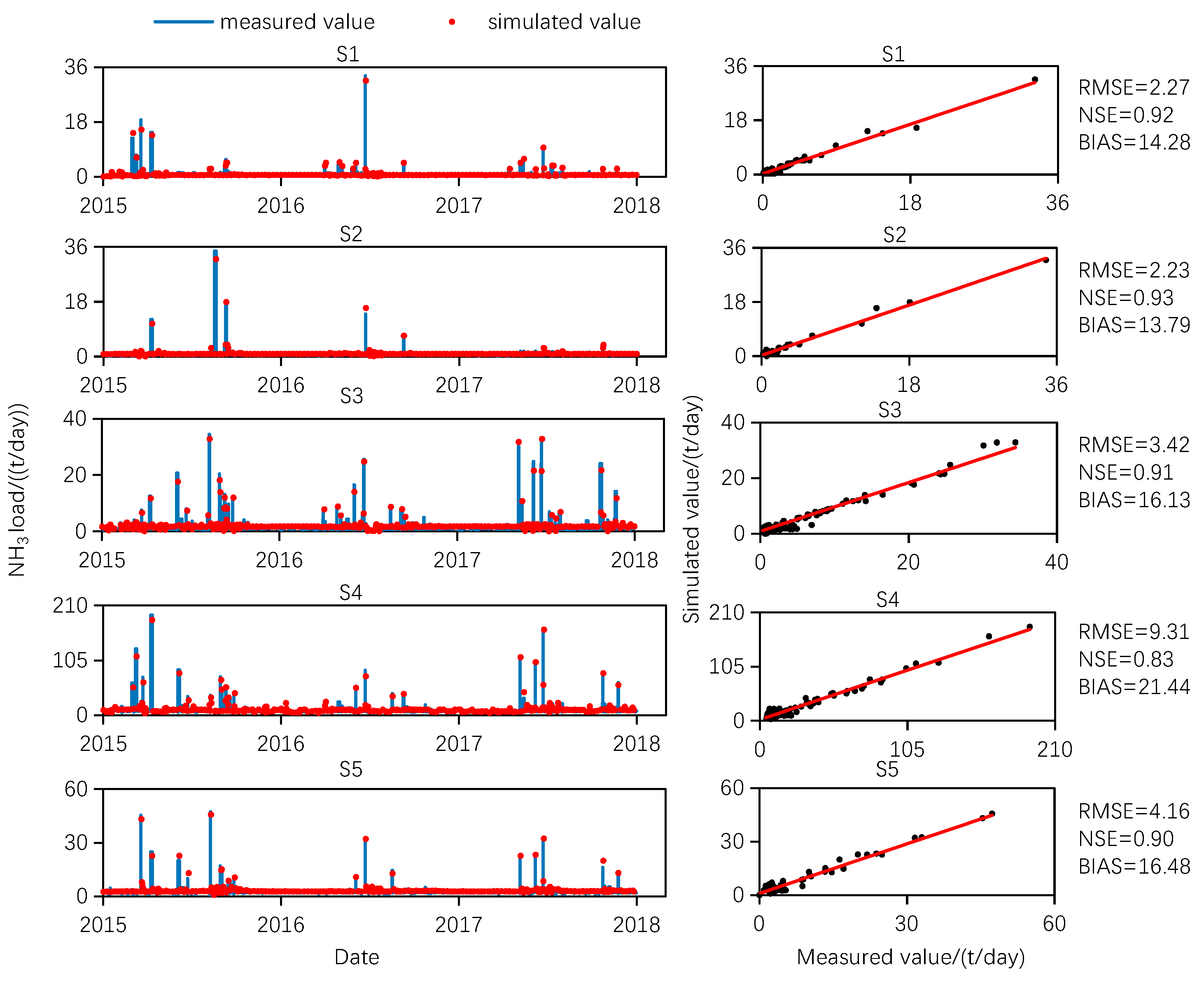
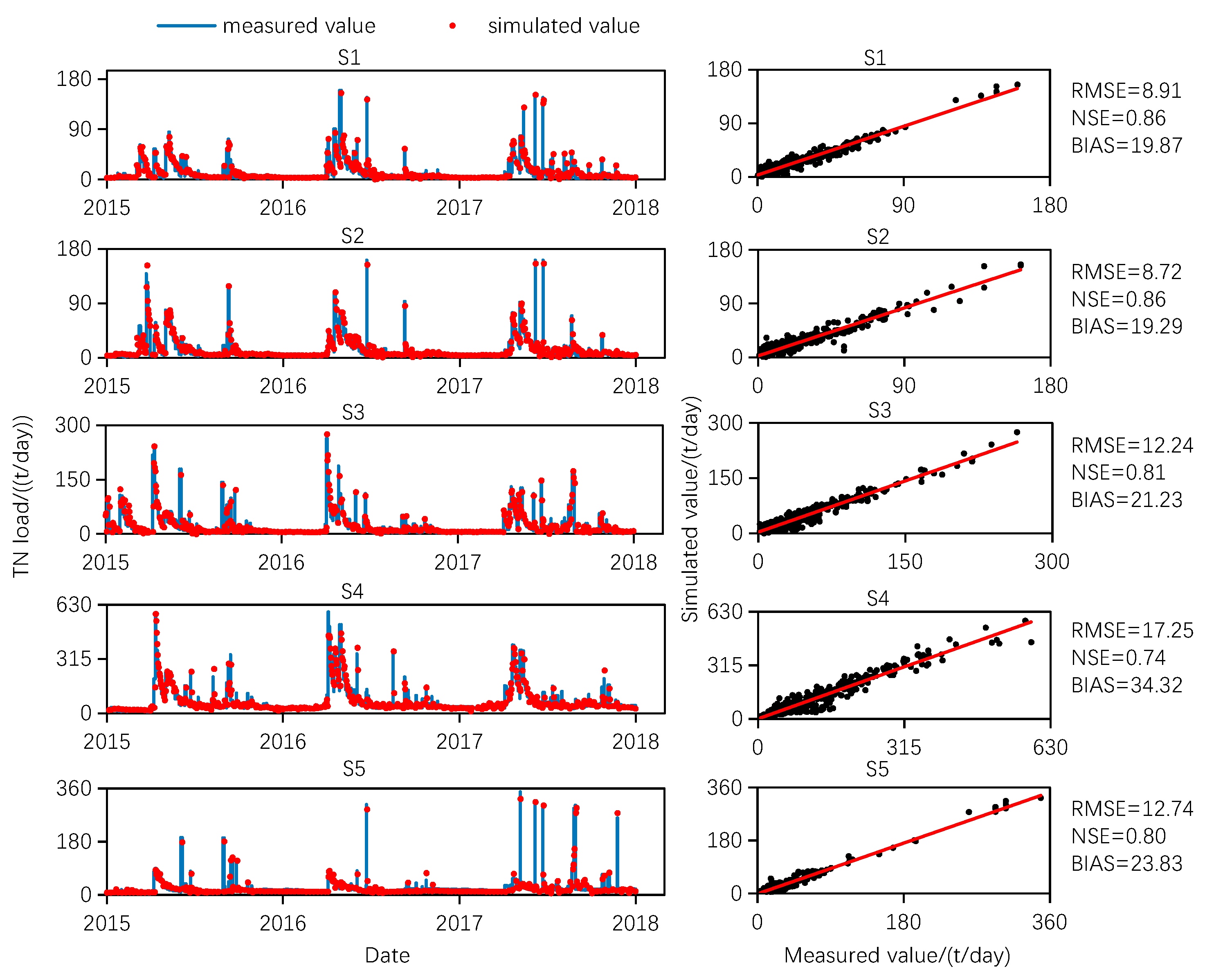
The comparison of the measured and LSTM-BP-simulated NH₃ and TN load on the validation set are shown in Figure 7 and Figure 8, respectively. Although the variation of the simulated pollution load with the LSTM-BP model was high under different hydrological periods (Table 4) and precipitation intensities (Table 5), the LSTM-BP model could track the temporal variation trend of the pollution load accurately. Since these temporal variations may result from pollutant transport characteristics [11], this result implies that the LSTM-BP model can better reflect the transport characteristics of pollutants. These temporal variation have been well simulated in previous studies. For example, Baek et al. [11] simulated the temporal variation of TN, TP and TOC concentration using the LSTM model with the NSE value of 0.987, 0.899 and 0.832, respectively.

4. Conclusions

This study developed a data-driven model based on LSTM-BP spatiotemporal combination for the simulation of pollution load at basin scale. The model comprised several time simulators based on LSTM and a spatial combiner based on BP. The model was applied in the Zhouhe River basin. Results showed that there is a high spatial correlation (i.e., Pearson’s correlation coefficient is larger than 0.5) in the pollution load between nearby sub-basins. The strong spatial correlation supports using a single model to simulate the pollution load at all sub-basins, rather than independent models for each sub-basin. Moreover, the performance of the LSTM model is better than that of the BP model and the LSTM model can achieve comparable performance with the SWAT model in most cases, whereas the performance of the LSTM-BP model is much better than that of the LSTM and SWAT models. Besides, the BP, LSTM, LSTM-BP and SWAT models underestimate the TN peak, which leads to a better simulation of NH₃ load than TN load. Although the variation of the simulated pollution load with the LSTM-BP model is high under different hydrological periods and precipitation intensities, the LSTM-BP model can track the temporal variation trend of the pollution load accurately (i.e., the RMSE is 6.27, NSE is 0.86 and BIAS is 19.46 for the NH₃ load and the RMSE is 20.27, NSE is 0.71 and BIAS 36.87 is for the TN load). The results of this study demonstrate the applicability of data-driven models, especially the LSTM-BP model, in the simulation of pollution load at basin scale. Although the developed model showed the acceptable simulation performance, only NH₃ load and TN load were simulated in this study. However, most physical models can simulate a variety of pollution load (i.e., total phosphorus, chemical oxygen demand and dissolved oxygen). Therefore, a further study to data-driven models is recommended to simulate more pollutants. Besides, this study only considers the pollution load simulation for the next day t, so multi-scale pollution load simulation can be considered in the future study, such as the variation trend simulation of pollution load in the next seven days.

References

- Chang, C.L.; Li, M.Y. Predictions of diffuse pollution by the HSPF model and the Back-Propagation neural network model. Water Environ. Res. 2017, 89, 732–738. [Google Scholar] [CrossRef]
- Albek, M.; Albek, E.A.; Göncü, S.; Uygun, B.S. Ensemble streamflow projections for a small watershed with HSPF model. Environ. Sci. Pollut. Res. 2019, 26, 36023–36036. [Google Scholar] [CrossRef]
- Kim, T.G.; Choi, K.-S. A study on water quality change by land use change using HSPF. Environ. Eng. Res. 2019, 25, 123–128. [Google Scholar] [CrossRef]
- Bouslihim, Y.; Rochdi, A.; Paaza, N.E.A.; Liuzzo, L. Understanding the effects of soil data quality on SWAT model performance and hydrological processes in Tamedroust watershed (Morocco). J. Afr. Earth Sci. 2019, 160, 103616. [Google Scholar] [CrossRef]
- Xie, K.; Liu, P.; Zhang, J.Y.; Libera, D.A.; Wang, G.Q.; Li, Z.J.; Wang, D.B. Verification of a new spatial distribution function of soil water storage capacity using conceptual and SWAT models. J. Hydrol. Eng. 2020, 25, 04020001. [Google Scholar] [CrossRef]
- Hu, J.; Ma, J.; Nie, C.; Xue, L.Q.; Zhang, Y.; Ni, F.Q.; Deng, Y.; Liu, J.S.; Zhou, D.K.; Li, L.H.; et al. Attribution analysis of runoff change in Min-Tuo River basin based on SWAT model simulations. Sci. Rep. 2020, 10, 401–408. [Google Scholar] [CrossRef] [PubMed] [Green Version]
- Abdelwahab, O.M.M.; Bingner, R.L.; Milillo, F.; Gentile, F. Evaluation of alternative management practices with the AnnAGNPS model in the Carapelle watershed. Soil Sci. 2016, 181, 293–305. [Google Scholar] [CrossRef]
- Karki, R.; Tagert, M.L.M.; Paz, J.O.; Bingner, R.L. Application of AnnAGNPS to model an agricultural watershed in East-Central Mississippi for the evaluation of an on-farm water storage (OFWS) system. Agric. Water Manag. 2017, 192, 103–114. [Google Scholar] [CrossRef]
- Upadhyay, P.; Pruski, L.O.S.; Kaleita, A.L.; Soupir, M.L. Evaluation of AnnAGNPS for simulating the inundation of drained and farmed potholes in the Prairie Pothole Region of Iowa. Agric. Water Manag. 2018, 204, 38–46. [Google Scholar] [CrossRef]
- Noori, N.; Kalin, L.; Isik, S. Water quality prediction using SWAT-ANN coupled approach. J. Hydrol. 2020, 590, 125220. [Google Scholar] [CrossRef]
- Baek, S.-S.; Pyo, J.; Chun, J.A. Prediction of water level and water quality using a CNN-LSTM combined deep learning approach. Water 2020, 12, 3399. [Google Scholar] [CrossRef]
- Fan, H.; Jiang, M.; Xu, L.; Zhu, H.; Cheng, J.; Jiang, J. Snowmelt-Driven Streamflow Prediction Using Machine Learning Techniques (LSTM, ARX, GPR and SVR). Water 2020, 12, 175. [Google Scholar] [CrossRef] [Green Version]
- Behzad, M.; Asghari, K.; Eazi, M.; Palhang, M. Generalization performance of support vector machines and neural networks in runoff modeling. Expert Syst. Appl. 2009, 36, 7624–7629. [Google Scholar] [CrossRef]
- Katimon, A.; Shahid, S.; Mohsenipour, M. Modeling water quality and hydrological variables using ARIMA: A case study of Johor River, Malaysia. Sustain. Water Resour. Manag. 2018, 4, 991–998. [Google Scholar] [CrossRef]
- Lin, H.; Kang, Y.B.; Wang, D.Y.; Lu, Z.Y.; Tian, W.; Wang, S.Q. Forecast of water quality along the Luanhe River line based on BP neural network. Iop Conf. Ser. Earth Environ. Sci. 2019, 267, 032075. [Google Scholar] [CrossRef]
- Frate, F.D.; Ferrazzoli, P.; Schiavon, G. Retrieving soil moisture and agricultural variables by microwave radiometry using neural networks. Remote Sens. Environ. 2003, 84, 174–183. [Google Scholar] [CrossRef]
- Parkin, G.; Birkinshaw, S.J.; Younger, P.L.; Rao, Z.; Kirk, S. A numerical modelling and neural network approach to estimate the impact of groundwater abstractions on river flows. J. Hydrol. 2007, 339, 15–28. [Google Scholar] [CrossRef]
- Feng, R. Prediction of Runoff Series in Jiulong River Basin Based on LSTM Model. Master’s Thesis, Changan University, Xi’an, Shaanxi, China, 2019. [Google Scholar]
- Qiao, B.; Fang, K.; Chen, Y.M.; Zhu, X.H.; He, X.P. Wavelet-Recurrent neural network (RNN): A real-time denoising technology for water quality sensor data. J. Nanoelectron. Optoelectron. 2019, 14, 497–504. [Google Scholar] [CrossRef]
- Wang, Y.Y.; Zhou, J.; Chen, K.J.; Wang, Y.Y.; Liu, L.F. Water quality prediction method based on LSTM neural network. In Proceedings of the 12th International Conference on Intelligent Systems and Knowledge Engineering, Nanjing, China, 24–26 November 2017; pp. 1–5. [Google Scholar]
- Fang, K.; Shen, C.P.; Kifer, D.; Yang, X. Prolongation of SMAP to spatiotemporally seamless coverage of continental U.S. using a deep learning neural network. Geophys. Res. Lett. 2017, 44, 11–30. [Google Scholar] [CrossRef] [Green Version]
- Zhou, J.; Wang, Y.Y.; Xiao, F.; Wang, Y.Y.; Sun, L.J. Water quality prediction method based on IGRA and LSTM. Water 2018, 10, 1148. [Google Scholar] [CrossRef] [Green Version]
- Hochreiter, S.; Schmidhuber, J. Long short-term memory. Neural Comput. 1997, 9, 1735–1780. [Google Scholar] [CrossRef]
- Hu, C.; Wu, Q.; Li, H.; Jian, S.; Li, N.; Lou, Z. Deep Learning with a Long Short-Term Memory Networks Approach for Rainfall-Runoff Simulation. Water 2018, 10, 1543. [Google Scholar] [CrossRef] [Green Version]
- Kratzert, F.; Klotz, D.; Brenner, C.; Schulz, K.; Herrnegger, M. Rainfall-runoff modeling using long short-term memory (LSTM) networks. Hydrol. Earth Syst. Sci. 2018, 22, 6005–6022. [Google Scholar] [CrossRef] [Green Version]
- Lai, X.; Gong, Y.F.; Cen, S.X.; Tian, H.; Zhang, H. Impact of the westerly jet on rainfall/runoff in the source region of the Yangtze River during the flood season. Adv. Meteorol. 2020, 6726347. [Google Scholar] [CrossRef] [Green Version]
- Wrb, I.W.G. World reference base for soil resources 2014. In International Soil Classification System for Naming Soils and Creating Legends for Soil Maps; FAO: Rome, Italy, 2015. [Google Scholar]
- Pereira, S.; Reynders, E.; Magalhães, F.; Cunha, Á.; Gomes, J.P. The role of modal parameters uncertainty estimation in automated modal identification, modal tracking and data normalization. Eng. Struct. 2020, 224, 111208. [Google Scholar] [CrossRef]
- Okada, S.; Ohzeki, M.; Taguchi, S. Efficient partition of integer optimization problems with one-hot encoding. Sci. Rep. 2019, 9, 13036. [Google Scholar] [CrossRef] [PubMed]
- Li, X.; Peng, L.; Yao, X.J.; Cui, S.L.; Hu, Y.; You, C.Z.; Chi, T.H. Long short-term memory neural network for air pollutant concentration predictions: Method development and evaluation. Environ. Pollut. 2017, 231, 997–1004. [Google Scholar] [CrossRef] [PubMed]
- Peng, H.; Wu, H.; Wang, J.W.; Dede, T. Research on the prediction of the water demand of construction engineering based on the BP neural network. Adv. Civ. Eng. 2020, 8868817. [Google Scholar] [CrossRef]
- Moriasi, D.N.; Arnold, J.G.; Van Liew, M.W.; Bingner, R.L.; Harmel, R.D.; Veith, T.L. Model evaluation guidelines for systematic quantification of accuracy in watershed simulations. Trans. Asabe 2007, 50, 885–900. [Google Scholar] [CrossRef]
- Wang, K.; Wang, P.; Zhang, R.; Lin, Z. Determination of spatiotemporal characteristics of agricultural non-point source pollution of river basins using the dynamic time warping distance. J. Hydrol. 2020, 583, 124303. [Google Scholar] [CrossRef]
- Parks, S.J.; Baker, L.A. Sources and transport of organic carbon in an Arizona river-reservoir system. Water Res. 1997, 31, 1751–1759. [Google Scholar] [CrossRef]
- Alamdari, N.; Sample, D.J.; Steinberg, P.; Ross, A.C.; Easton, Z.M. Assessing the effects of climate change on water quantity and quality in an urban watershed using a calibrated stormwater model. Water 2017, 9, 464. [Google Scholar] [CrossRef]
- Karlen, D.L.; Dinnes, D.L.; Jaynes, D.B.; Hurburgh, C.R.; Cambardella, C.A.; Colvin, T.S.; Rippke, G.R. Corn response to late-spring nitrogen management in the Walnut Creek watershed. Agron. J. 2005, 97, 1054–1061. [Google Scholar] [CrossRef] [Green Version]
- Zheng, T.; Mu, H.; Huang, Y.; Zhang, C. Smiulated research on decreasing pollution loads in rainfall runoff with accelerating infiltration. Tech. Equip. Environ. Pollut. Control 2006, 7, 84–88. [Google Scholar]
- Schrumpf, M.; Zech, W.; Lehmann, J.; Lyaruu, H.V. TOC, TON, TOS and TOP in rainfall, throughfall, litter percolate and soil solution of a montane rainforest succession at Mt. Kilimanjaro, Tanzania. Biogeochemistry 2006, 78, 361–387. [Google Scholar] [CrossRef]
- Park, M.; Choi, Y.S.; Shin, H.J.; Song, I.; Yoon, C.G.; Choi, J.D.; Yu, S.J. A comparison study of runoff characteristics of non-point source pollution from three watersheds in South Korea. Water 2019, 11, 966. [Google Scholar] [CrossRef] [Green Version]
- Zhao, J.; Deng, F.; Cai, Y.; Chen, J. Long short-term memory-Fully connected (LSTM-FC) neural network for PM2.5 concentration prediction. Chemosphere 2019, 220, 486–492. [Google Scholar] [CrossRef]
Figure 1.
Basic information of the Zhouhe River basin. (a) Location of the Zhouhe River basin; (b) Land use; (c) Soil type; (d) Soil total nitrogen (TN) content.
Figure 2.
Values of monthly NH3 load and precipitation on the validation set.
Figure 3.
Values of monthly TN load and precipitation on the validation set.
Figure 4.
Long Short-Term Memory (LSTM)-based temporal simulator.
Figure 5.
Back Propagation (BP)-based spatial combinatory.
Figure 6.
Illustration of the Long-Short Term Memory (LSTM)-Back Propagation (BP) model structure for simulating pollution load at basin scale.
Figure 7.
Comparison of the measured and LSTM-BP-simulated NH3 load on the validation set.
Figure 8.
Comparison of the measured and LSTM-BP-simulated TN load on the validation set.