
Controls on Streamflow Densities in Semiarid Rocky Mountain Catchments
by
 , ,
, ,
Caroline Martin
1,2, 
Stephanie K. Kampf
1,*,
John C. Hammond
1,3,
Codie Wilson
4 and
Suzanne P. Anderson
5 1
Department of Ecosystem Science and Sustainability, Colorado State University, Fort Collins, CO 80523, USA
2
Now at TCarta Marine LLC, Denver, CO 80204, USA
3
Now at U.S. Geological Survey, MD-DE-DC Water Science Center, Catonsville, MD 21228, USA
4
Natural Resources Ecology Laboratory, Colorado State University, Fort Collins, CO 80523, USA
5
Department of Geological Sciences, and Institute of Arctic and Alpine Research, University of Colorado, Boulder, CO 80309, USA
*
Author to whom correspondence should be addressed.
Water 2021, 13(4), 521; https://doi.org/10.3390/w13040521
Submission received: 30 November 2020
/
Revised: 11 February 2021
/
Accepted: 13 February 2021
/
Published: 17 February 2021
(This article belongs to the Special Issue Hydrology, Geomorphology, and Ecology of Intermittent Rivers and Streams)
Abstract
:Developing accurate stream maps requires both an improved understanding of the drivers of streamflow spatial patterns and field verification. This study examined streamflow locations in three semiarid catchments across an elevation gradient in the Colorado Front Range, USA. The locations of surface flow throughout each channel network were mapped in the field and used to compute active drainage densities. Field surveys of active flow were compared to National Hydrography Dataset High Resolution (NHD HR) flowlines, digital topographic data, and geologic maps. The length of active flow declined with stream discharge in each of the catchments, with the greatest decline in the driest catchment. Of the tributaries that did not dry completely, 60% had stable flow heads and the remaining tributaries had flow heads that moved downstream with drying. The flow heads were initiated at mean contributing areas of 0.1 km2 at the lowest elevation catchment and 0.5 km2 at the highest elevation catchment, leading to active drainage densities that declined with elevation and snow persistence. The field mapped drainage densities were less than half the drainage densities that were represented using NHD HR. Geologic structures influenced the flow locations, with multiple flow heads initiated along faults and some tributaries following either fault lines or lithologic contacts.
1. Introduction
Headwater streams are dynamic, expanding and contracting seasonally and in response to rain and snowmelt. Parts of the channel network that do not flow continuously in time are called intermittent; these streams make up an estimated 50–70% of stream length in the United States [1,2] and greater than 50% globally [1]. These discontinuous streams are important contributors to biodiversity, material transport, and water supply for larger streams and water bodies [3], yet they are typically not as well mapped or monitored as larger perennial streams. Information on stream location and flow duration may be used to determine whether streams are protected by water quality regulations or land management guidelines. Researchers and land managers typically rely on public hydrography data for mapping stream networks, and these stream maps are then used in models that quantify the water fluxes, water quality, or landscape evolution. For example, the National Hydrography Dataset (NHD) is a publicly available river network dataset for the United States that was created to assist scientists and land managers in modeling hydrologic features, water quantity, and water quality. The NHD streams were initially digitized from United States Geological Survey (USGS) 1:100,000 scale topographic maps; NHD streams are now available at 1:24,000 scale as well [4]. However, given the substantial length of headwater streams, most have not been mapped through direct field surveys. Consequently, hydrography datasets can be inaccurate, particularly for the smallest headwater streams [5,6,7]. A better understanding of the factors driving streamflow locations would help to improve the accuracy of current hydrography data.
Two key components are needed to map and classify streams: the locations of stream channels and the duration of flow within these channels. Stream channels are geomorphic features in which water flow and sediment transport are concentrated between definable banks and they initiate at the geomorphic channel head [8]. Stream channels are more permanent geomorphic features than rills, which are created by ephemeral surface erosion, but channels defined as streams do not necessarily always contain flowing water [9]. Here, we distinguish between the geomorphic channel network and the portion of that network that contains active flow. The actively flowing portion of the channel network may expand and contract with changes in the streamflow, making it more dynamic than the geomorphic channel network [10,11,12,13,14,15,16,17,18]. Both geomorphic and active channel lengths can be used to compute drainage densities. Here, we define the geomorphic drainage density (GDD) as the total geomorphic channel length divided by the drainage area and the active drainage density (ADD) [18] as the flowing channel length divided by the drainage area. Both the GDD and ADD have been referred to in the literature as simply “drainage density,” although some studies use modified terms for the ADD, including wetted channel drainage density [15]. In most cases, the ADD is less than or equal to the GDD because it includes only the portion of the geomorphic channel network that is flowing; however, including diffuse overland flow paths can make the ADD greater than the GDD [13,19].
The GDD is related to both climate and geology. Abrahams and Ponczynski [20] found that GDD decreases with greater mean annual precipitation in dry climates up to around 1000 mm. This may be because more precipitation leads to increased vegetative cover, which suppresses erosion and channel incision [21]. However, in wetter climates, the GDD tends to increase with mean annual precipitation due to greater amounts of water exported as runoff [22,23]. The effects of climate on the ADD are not consistent, as some of the highest reported values have been in both humid climates with saturation overland flow [13] and semiarid climates with infiltration-excess overland flow [24]. The amount of change in the ADD also varies substantially between sites with different climates [25]. The ADD of some channel networks varies by orders of magnitude, ranging from < 1 km km−2 to > 10 km km−2 at a given location [13,24,26]: higher drainage densities are often associated with saturation overland flow, which can dramatically increase the ADD in catchments with shallow water tables. At other catchments, the ADD varies moderately by factors of 2–3 [12,14,18,26] or is relatively stable due to fixed spring water sources for the channel flow [15,27].
Within climatic regions, multiple studies have documented the important role of bedrock geology on the ADD. The ADD tends to be lower over unconsolidated sediments or highly permeable bedrock, which allow for more infiltration as compared to locations with rock outcrops and shallow soils [18]. However, the effects of lithology on the drainage density are not consistent between locations. At study sites in the Appalachians, sedimentary lithologies had lower ADDs than metamorphic lithologies [26], whereas at a study area in New South Wales, sedimentary lithologies had a higher ADD than granitic lithologies [24]. Differences in lithology within a catchment can lead to spatial discontinuities in the flow, particularly where streams transition from less permeable to more permeable geologic units [27]. Weathered and fractured bedrock may provide storage of water that can be gradually released to channels [15], while structural features, such as joints, faults, or lithologic contact zones, may be associated with springs that initiate channel flow [27,28].
Topography is a strong indicator of where channels are located [29]; therefore, topographic algorithms are frequently used to map channel networks [30,31,32]. Often, such approaches use thresholds of the drainage area (A) or the topographic wetness index (TWI) [33], which involves mapping channel locations as all grid cells with values higher than the threshold. Threshold values can vary considerably for different locations and applications [34,35,36], as well as for different digital elevation model (DEM) resolutions [37,38,39,40,41,42,43,44,45]. Channel networks derived from topographic data alone are not always accurate [11,34,46] because locations of small headwater streams can also be influenced by geology, soil, and vegetation [6,47,48,49]. To account for these factors, some studies have applied more detailed statistical models to map channel locations as functions of topography, as well as other variables, such as precipitation, land cover, and geology [35,50,51].
Because the factors affecting active flow locations vary substantially between sites, improvements in hydrographic datasets will require extensive field campaigns that document the flow in channel networks across a range of climatic, geologic, and land cover conditions. This study examined the dynamics of the flowing channel networks for three semiarid catchments along an elevation gradient in the Colorado Front Range, USA, and compared these to the channel networks in the National Hydrography Dataset. The research objectives were to (1) determine where surface streams were actively flowing in these catchments during early and late summer, (2) evaluate how field-mapped streams compared to those derived from the surface topography and NHD, and (3) assess how active flow locations related to the geology and the climate gradient between sites.
2. Materials and Methods
2.1. Study Sites
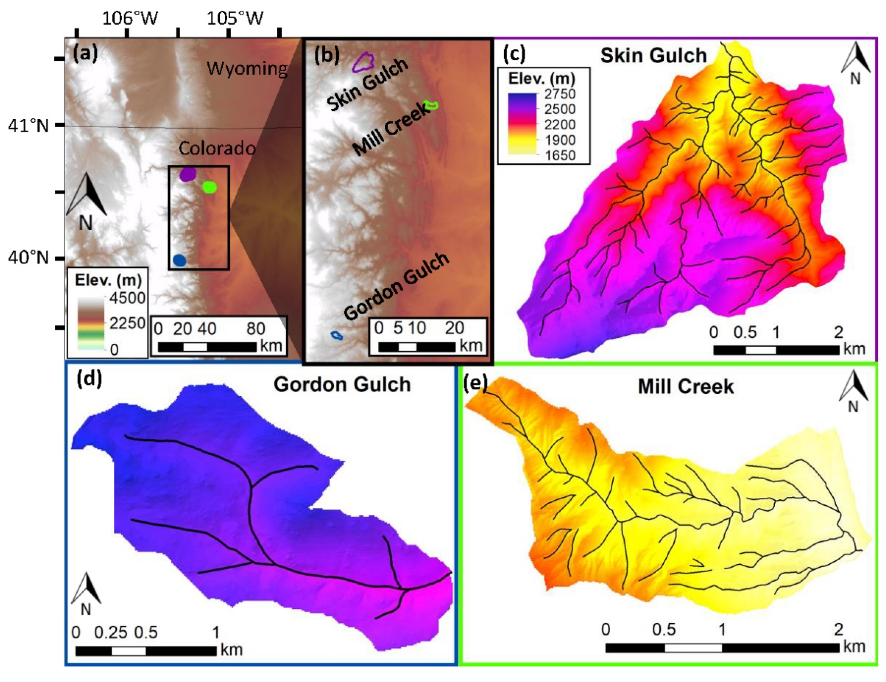
The study region was the Colorado Front Range on the eastern slope of the Rocky Mountains, USA. Three natural catchments with no flow modifications were monitored along the mountain front (Figure 1). The lowest elevation catchment, Mill Creek, has a 3.8 km2 drainage area and ranges in elevation from 1651 to 2166 m (Table 1). The slope average is 21°, with steeper slopes up to 62° along the bedrock outcrops bounding the main channel. The resistant steep bedrock consists of mostly metamorphic schist [52] (Figure 2). Bedrock in the catchment also includes felsic intrusive rocks. The lower part of the catchment spans the lithologic contact between old Precambrian and younger Permian sedimentary layers, which include a coarse sedimentary conglomerate near the catchment outlet. Positioned near the mountain front, where the Rocky Mountains uplift initiates, the base level of Mill Creek is tied to the incision of the plains to the east. The soils are mainly sandy loams in the upper part of the catchment, with a band of loamy soils at lower elevations. Vegetation is primarily shrubs and grasses at the lowest elevations, ponderosa pine (Pinus ponderosa) at middle elevations, and patches of mixed conifers at the highest elevations. Mill Creek has a mean annual precipitation (P) of 464 mm, as determined from the gridded precipitation data product, PRISM [53], and mean annual potential evapotranspiration (PET) of 1245 mm, as estimated from the gridded reference evapotranspiration product in gridMET [54]. This gives an aridity index (P/PET) of 0.37. The catchment experiences intermittent winter snow cover, and the main channel is an intermittent stream that flows mainly during winter, spring, and early summer.
The middle-elevation catchment, Skin Gulch, has a 15.5 km2 drainage area, with an elevation ranging from 1841 to 2682 m and an average slope of 22°. The stream drains into the Cache la Poudre River, which sets the base elevation for the catchment. The bedrock geology is a combination of Precambrian metamorphic schist, amphibolite, and intrusive granodiorite and pegmatites (Figure 3). This area is structurally diverse; it includes a shear zone from the northeast to the southwest and the Stove Prairie fault that runs northwest to southeast [55]. The soil is mainly Redfeather sandy loam. Vegetation in the catchment is diverse, including shrubland and ponderosa pine at lower elevations and mixed conifer, with patches of aspen and lodgepole pine (Pinus contorta) at the higher elevations. The mean annual P across Skin Gulch is 516 mm [53] and the mean annual PET is 1135 mm [54], giving an aridity index (P/PET) of 0.45. Most of the catchment experiences intermittent snow cover, but snow persists through the winter at the higher elevations. Much of Skin Gulch was burned at a moderate–high severity in the 2012 High Park Fire [56], which resulted in extensive rill and gully erosion during the first two years after the fire [57,58]. Since the fire, the main channel has had perennial flow in the reach, draining to the catchment outlet [59].
The highest elevation catchment, Gordon Gulch, has a 2.6 km2 drainage area, with elevations ranging from 2432 to 2733 m and an average slope of 14°. Gordon Gulch is on the Rocky Mountain Surface [60] and has not experienced base-level perturbations since the Pliocene. The geology is a mixture of Precambrian metamorphic and intrusive rocks [61]. Bedrock outcrops are common on hillslopes, with a slight preponderance of occurrence on south-facing slopes. Soils are mainly sandy loams with loam along the valley bottom; soil depths average 39 cm on slopes and reach up to 2 m at the base of north-facing slopes [62]. Vegetation at lower elevations and on south-facing slopes is primarily ponderosa pine, with lodgepole pine on north-facing and higher elevation slopes [63,64]. The mean annual precipitation is 511 mm [53] with 1166 mm of mean annual PET [54], giving an aridity index (P/PET) of 0.44. Snow persists through the winter at the higher elevations and on north-facing slopes but is more intermittent on south-facing slopes [65]. The streamflow is perennial at the outlet but intermittent at other locations, with the highest flow generally in spring and early summer.
2.2. Data and Analysis Methods
The stream networks of each catchment were each mapped twice during summer 2016 [66], which was a year with close-to-average annual precipitation (Table 2). Trip 1 was from June to mid-July and trip 2 was from mid-July to August (Table 2). For each catchment, surveys were completed within a week to avoid any large changes in the stream network during the survey. Surveys were conducted by foot following all branches of the channel network to document the presence or absence of flow using a combination of GPS waypoints and drawings of the active channel onto a topographic map. The flow was mapped where surface water was visibly connected longitudinally along a channel segment, whereas dry segments were mapped where no surface water was present in the channel. Pools with standing water and no visible longitudinal connection of the surface water were also mapped.
Stream discharge data for the catchment outlets (Table 2) were used to determine how long streams flowed for during the 2016 water year and to identify where on the hydrograph the field stream surveys were conducted. The discharge data for Skin Gulch and Mill Creek were collected by the authors [67], and the Gordon Gulch discharge was collected by Boulder Creek Critical Zone Observatory [68]. At each location, the stream stage was continuously measured using capacitance rods (WT-HR 1000 mm, TruTrack, Auckland, New Zealand) or pressure transducers (Rugged Troll 100, In Situ, Fort Collins, CO, USA; Levelogger, Solinst, Georgetown, ON, Canada). For each site, a stage–discharge rating curve was created based on the manual discharge measurements. The daily area-normalized discharge for each location was computed by dividing the discharge by the drainage area to facilitate a comparison of the different-sized catchments.
The topography for each site was characterized using 1 m resolution LiDAR digital elevation models (DEMs): the data for Mill Creek and Gordon Gulch were from the USGS [69] and the Skin Gulch data were from the National Ecological Observatory Network (NEON) [70]. For each catchment flow, flow accumulation grids used to determine drainage area (A) were computed using the D8 algorithm in ArcGIS Pro (Esri, Redlands, CA, USA). We also tried the D-infinity algorithm [71], but because the results were similar to the D8 results, we focused here only on D8. For each surveyed streamflow network, we extracted A values for the field mapped flow heads. We then developed stream networks by using the minimum, mean, and maximum A at each field-mapped flow head as the thresholds for stream initiation. We compared the topographically derived stream networks to the field-mapped networks and the National Hydrography Dataset High Resolution (NHD HR, 1:24,000) flowlines. For both the field and NHD HR channel networks, we computed the drainage density as the length of the channel divided by the drainage area. For the field-mapped channels, this density is equal to the ADD, whereas, for the NHD HR, it is theoretically the GDD, if the flowlines accurately map the channel network.
3. Results
3.1. Field Surveys
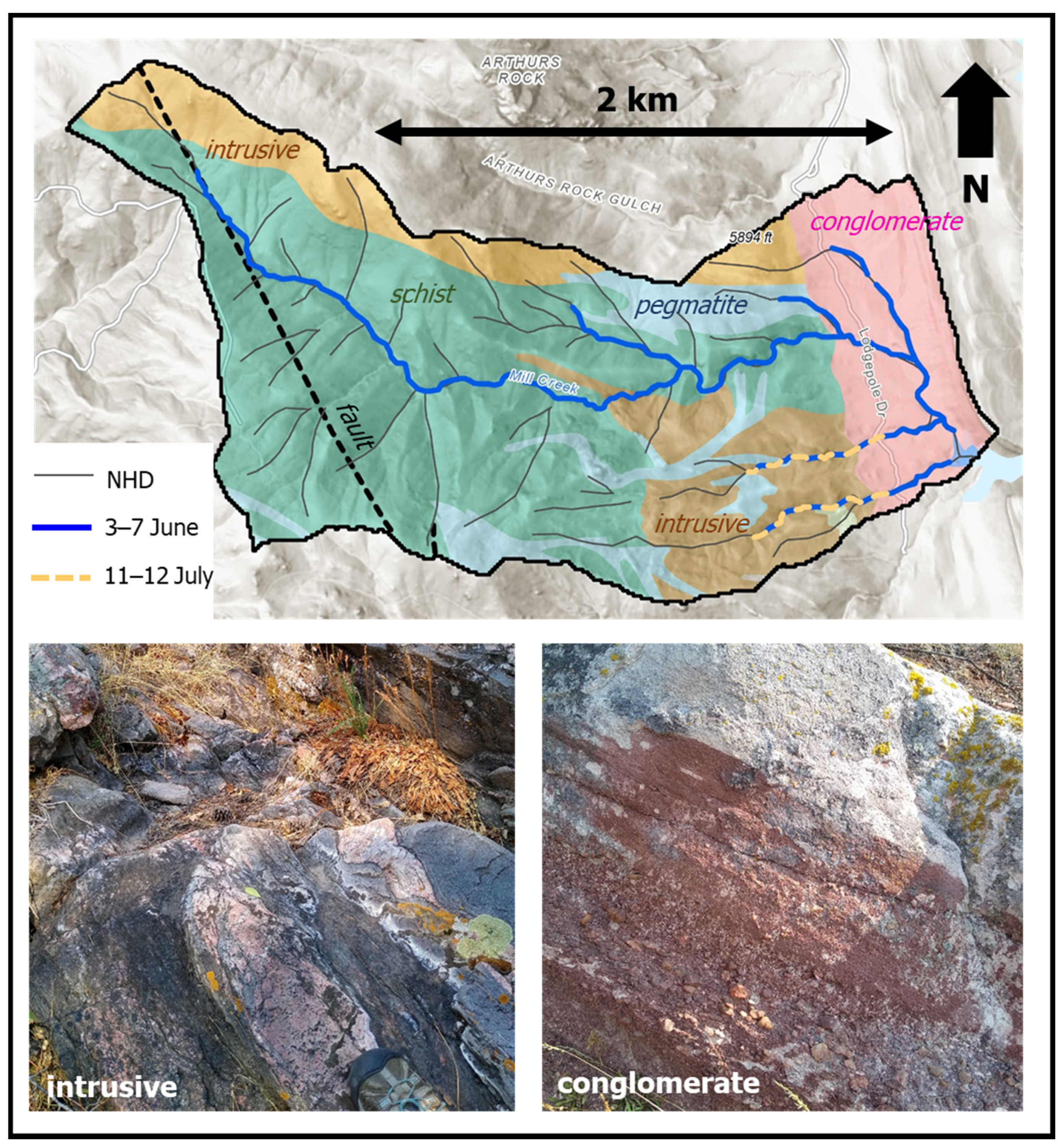
The flowing length of the streams varied temporally and spatially over the course of the two summer surveys (Figure 2, Figure 3 and Figure 4). Mill Creek had the greatest change in active stream length between surveys, decreasing 84% from a stream length of 6.9 km for the 3–7 June survey to 1.1 km for the 11–12 July survey (Figure 2). During the first survey, the flow in the main channel originated along a fault line and was continuous from this source area to the catchment outlet. Three tributaries north of the main channel and two tributaries south of the main channel were also flowing. During the second survey, only the two tributaries on the south side were flowing, and the entire main channel was dry. The two flowing tributaries originated in an area of intrusive bedrock, whereas the main channel of Mill Creek primarily overlays metamorphic schist. The location of the flow heads in these two southern tributaries remained the same for both field surveys; however, these streams dried downstream during the second survey as they flowed from the uplifted intrusive rock unit into flatter terrain over more permeable conglomerate bedrock (Figure 2).
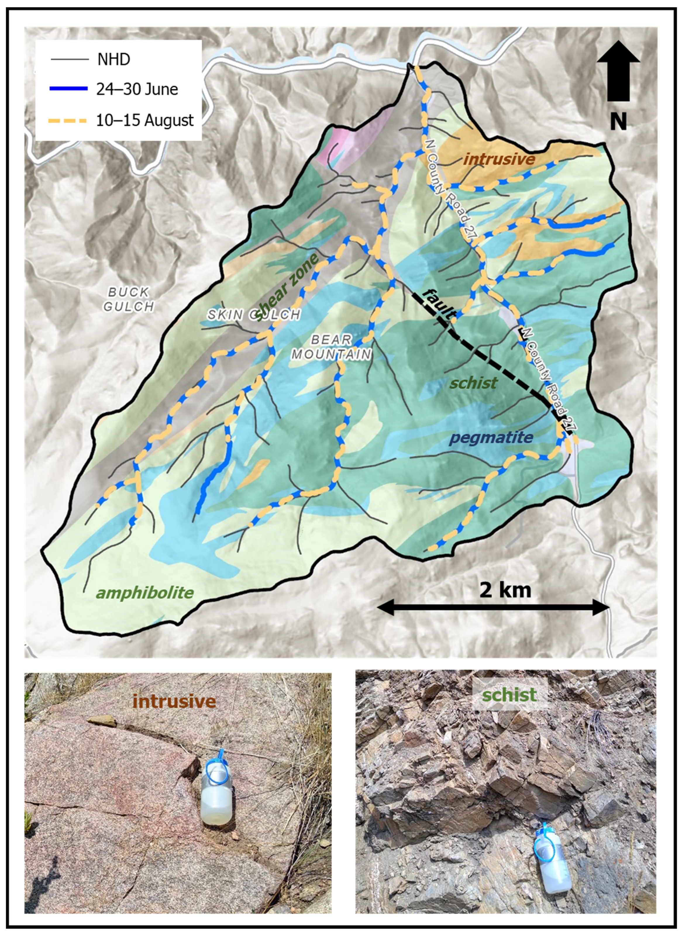
In contrast to Mill Creek, Skin Gulch had relatively little change in the actively flowing stream length for the two trips, with 20 km for trip 1 (late June) and a decrease in stream length of only 6% for the second trip (mid-August) (Figure 3). Six of the flow heads remained stable between the two field surveys and three channels contracted downstream. Both of the main channels in this catchment followed structural features, with the western channel following a shear zone and the eastern channel following a fault line. The tributaries on the northeastern side of the catchment followed contacts between the intrusive and metamorphic rocks.
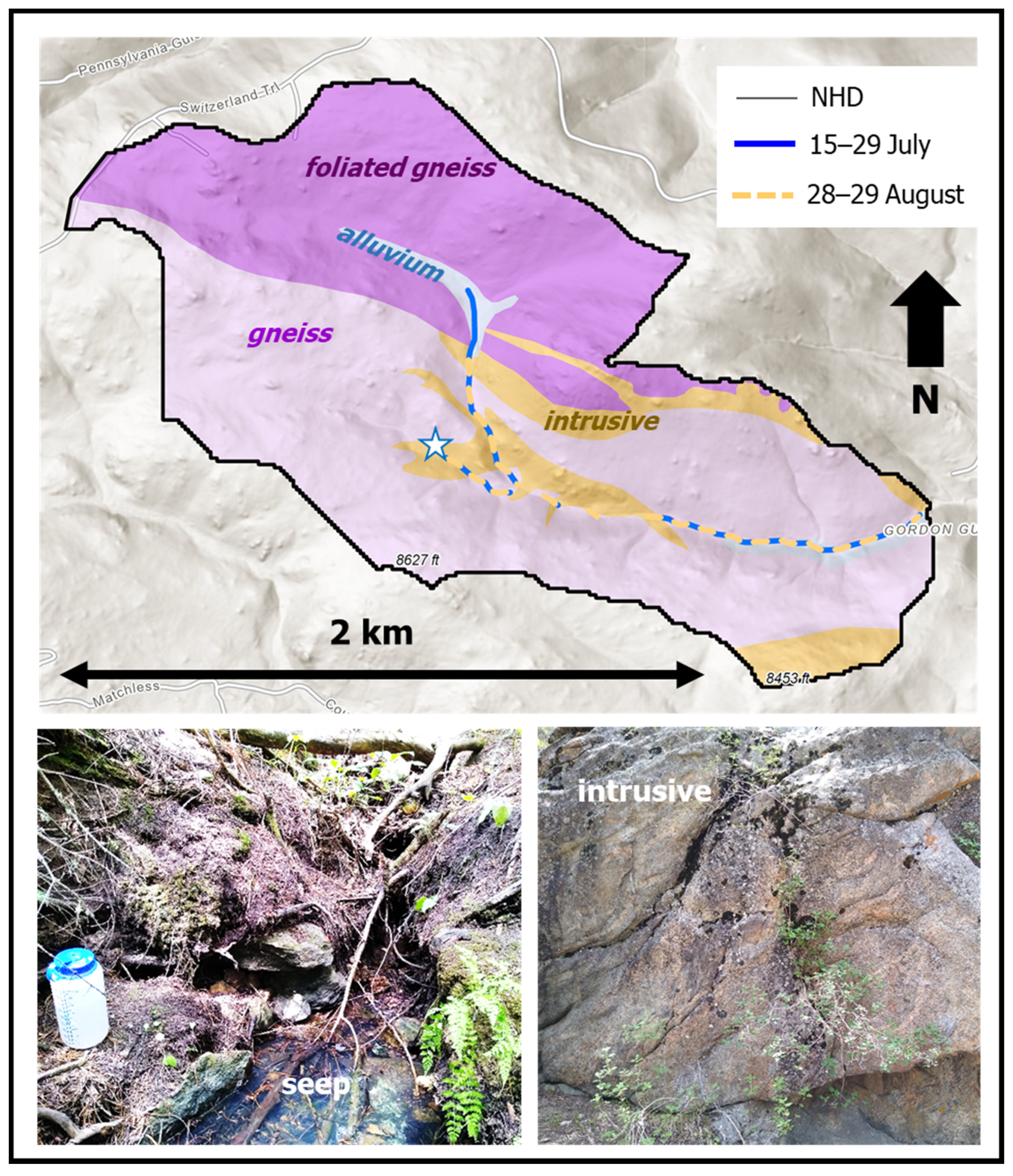
Gordon Gulch also had a relatively limited change in flowing channel length between the field surveys, with 1.9 km for the first survey in mid-July and a 13% decrease for the second survey in late August (Figure 4). The channel contracted along the northern tributary, whereas the flow head for the southern tributary remained stable. Gordon Gulch was the only catchment that had spatially discontinuous flow along the main stem. The discontinuous flow paths were located in a reach where the bedrock alternated between intrusive quartz monzonite and gneiss. However, the patterns of the flow presence and absence along the main stem were not clearly related to the lithologic changes; in some locations, the losses and gains of flow appeared to be related to the channel topography because the flow emerged below step drops in the channel bed elevation (Figure 4).
3.2. Catchment Comparison
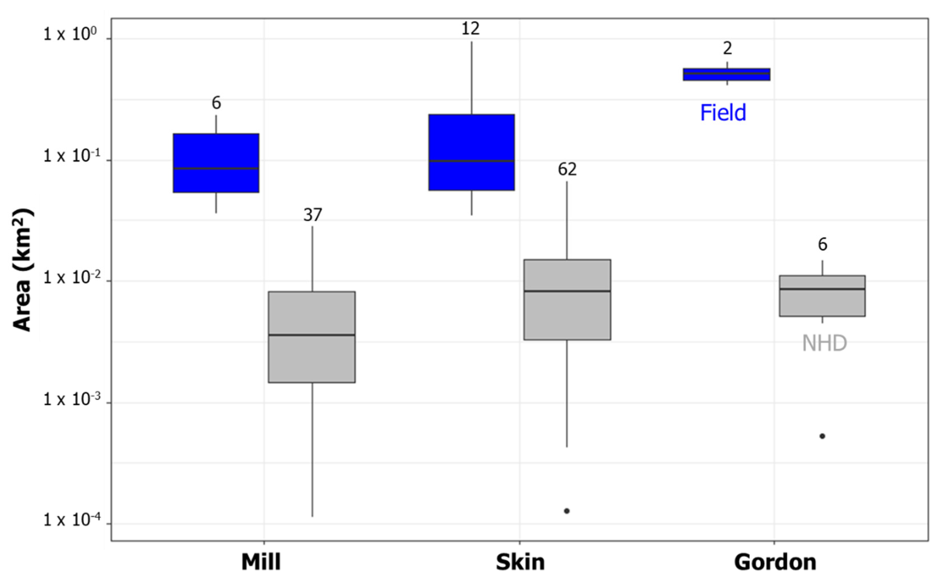
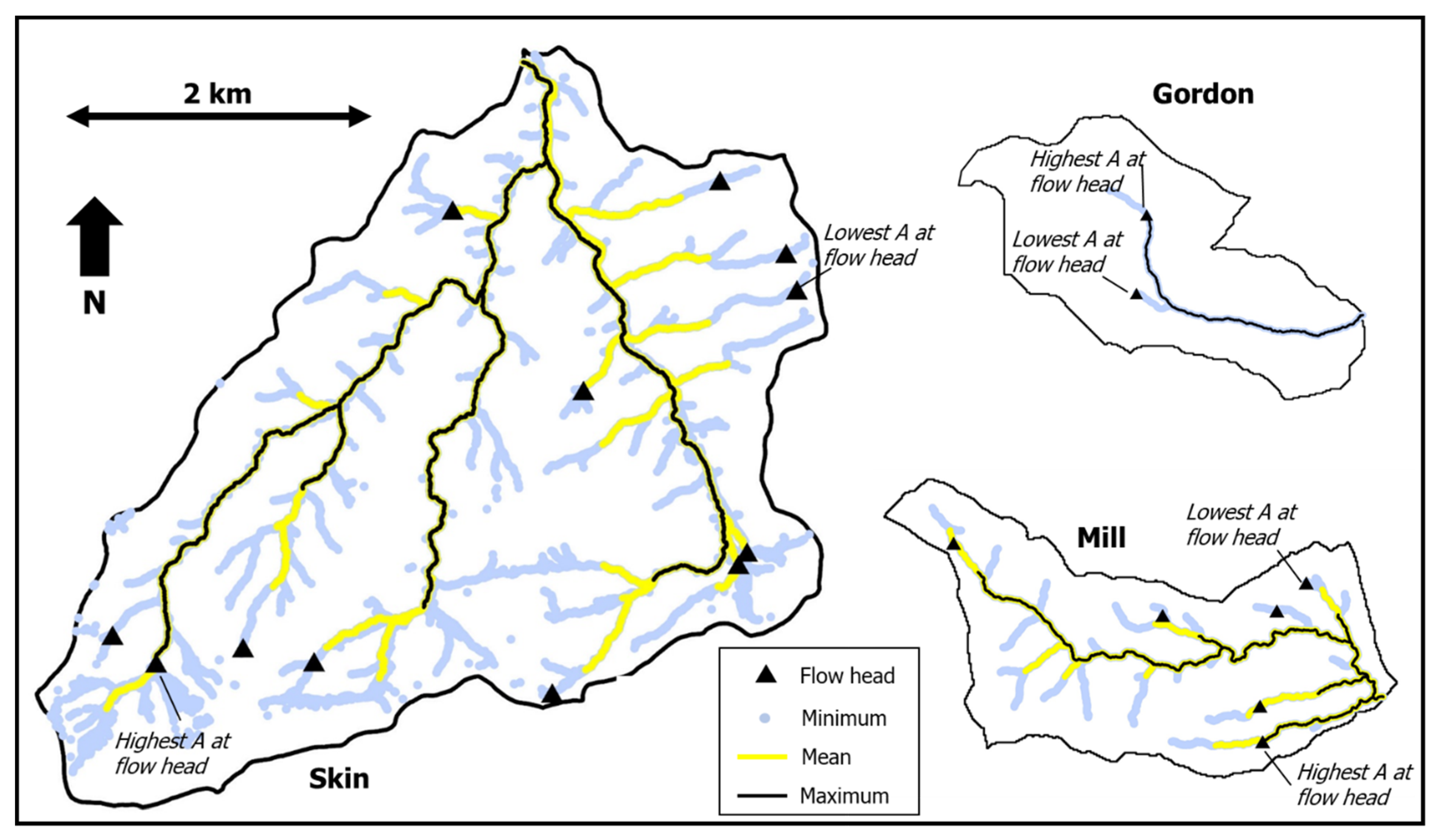
Flow heads were found at lower contributing areas for the lowest elevation site, Mill Creek (0.04–0.23 km2), compared to the highest elevation site, Gordon Gulch (0.41–0.64 km2). In Mill Creek, flow heads were found at the smallest contributing areas for the north-side tributaries and the largest contributing areas for the south-side tributaries, which were those that retained flow the longest through the summer. Skin Gulch covered a wider range of elevations and had flow heads at drainage areas from 0.04 to 0.95 km2 (Figure 5). The flow heads at the lower end of the contributing areas were mainly in the eastern, smaller tributaries at lower elevations, whereas the flow head with the highest contributing area was at the highest elevation main tributary in the southwestern corner of the catchment. This flow head emerged from below a grassy meadow that likely stored groundwater sourced from upstream hillslopes (Figure 6). The NHD channel heads were located at much lower drainage areas than the field-mapped flow heads, with drainage areas ranging from 0.0001 to 0.07 km2 (Figure 5).
Using the drainage area (A) values from the flow heads as thresholds for mapping stream channels led to spatial patterns of the streamflow that differed somewhat from the field surveys (Figure 6). For Mill Creek, when the mean A from the field channel heads was applied as a threshold for mapping flowing channels, the flow lengths were shorter than observed for some northern tributaries and longer than observed for the southernmost tributary. At Skin Gulch, the mean A from the field channel heads led to flow lengths that were too short on the eastern tributaries but too long on some of the southern headwater tributaries. Gordon Gulch had only two flow heads, both with similar A values. Using the smaller A to map streams led to a longer than observed headward extension of the main channel, whereas using the larger A omitted the southern tributary.
The differences in the drainage density between catchments mirrored their differences in the contributing areas at the flow heads. The ADD was the highest for Mill Creek during the first trip (1.83 km km−2) and the lowest for Gordon Gulch (0.69 km km−2), leading to a decline in the ADD with greater elevation and snow persistence (Figure 7a,c). This same elevation-dependent pattern for the ADD was not present for trip 2 because the lowest elevation site, Mill Creek, was mostly dry. The annual precipitation was similar for Mill Creek and Skin Gulch; therefore, the relationship between the ADD and precipitation (Figure 7b) was not as strong as those for the ADD vs. elevation and snow persistence (Figure 7a,c). The NHD GDD values were higher than the ADD values by a factor of two or more, but they also exhibited declines with increasing elevation. At each site, the ADD increased with discharge (Figure 7d), but this change was much larger for Mill Creek, where the channel network was mostly dry on the second trip, than for Skin Gulch and Gordon Gulch, which had only small changes in the discharge between trips. All surveys were conducted during hydrograph recessions and unfortunately started too late to capture peak flow conditions.
4. Discussion
4.1. Geologic Influences
In all three catchments, we found strong indications that the bedrock geology affected the stream channel locations and active flow patterns. In both Mill Creek and Skin Gulch, the flow in the main channels originated along fault lines, indicating that the faults may provide preferential pathways for subsurface flow to reach the surface. In Skin Gulch, these fault lines tracked with the channel, likely because the long-term erosion followed these paths of least resistance. This drainage pattern where the streams follow shear zones and faults is considered trellis drainage, and it is present in other surrounding watersheds as well. These observations agree with others [73] who found that areas along faults were more likely to be saturated than areas that are more distant from faults, and with other observations of springs and flow heads along faults [27,28]. Lithologic contacts also correspond with some of the stream locations in eastern Skin Gulch. Bedding contacts could also be considered a path of least resistance for water flow [74], and therefore, areas of preferential erosion.
The effect of lithology on active flow locations is difficult to disentangle from other controls on flow presence/absence. Other studies have found that lithologies with high hydraulic conductivities are more hydrologically connected [74,75] and documented greater active surface flow over less permeable lithologies [18,27]. These patterns appear to be consistent with our findings; however, in each catchment, there were multiple potential explanations for the patterns of flow presence/absence. In Mill Creek, we found that the tributaries with the longest flow duration were in locations with intrusive bedrock, whereas those in areas with schist or conglomerate bedrock lost flow earlier in the summer. However, the tributaries with a longer flow duration also had stable channel heads fed by seeps (Figure 2), and their flow may be sourced by groundwater that originated outside the small catchment boundaries [76]. In Skin Gulch, flowing tributaries on the east side of the catchment followed contacts between the granite and amphibolite, whereas many smaller tributaries over the schist bedrock did not have any mapped flow. However, the flowing tributaries were on slopes with west-facing aspects, in contrast to the east-facing aspects of the tributaries without flow. Gordon Gulch had a stretch of discontinuous flow corresponding with alternating intrusive and gneiss (banded) bedrock. However, the mixture of intrusives and gneiss in the catchment was quite intricate and only mapped based on the surface bedrock outcrops; therefore, there was not enough information to determine whether there was a lithologic role in flow locations.
Within the individual lithologies at all catchments, there may also be directional patterns in joints or foliation that affect the subsurface flow direction and the likelihood that the subsurface flow will emerge at the surface (e.g., Figure 3, schist). The architecture of weathering on the different lithologies, as well as sediment deposits from colluvium or landslides, will also affect the flow dynamics. Locations with thicker soils and/or weathered rock would have more storage capacity and permeability, and thus a lower ADD. Future work documenting regolith thicknesses in these catchments could provide more insights into drivers of flow patterns.
4.2. Topographic Thresholds
Because of the likely subsurface controls on flow emergence, topography-based thresholds for channelization may not work as well as they do in catchments where the water flows to channels through near-surface soils to produce a saturation overland flow [77,78]. We have not observed saturation overland flow in either of the low elevation catchments, and the soils at these sites generally do not reach saturation, even during wet spring conditions [79]. Unlike locations that do produce saturation overland flow, we found no consistent relationship between the drainage area and local slope at the flow heads for these study sites (Figure 8a). This is consistent with the findings of Henkle et al. [80], who mapped channel heads throughout the region and found that the relationship between the drainage area and local slope had an R2 of only 0.11. They suggested that spatial variations in the joint density may be responsible for subsurface flow locations that ultimately influenced the channel locations. For our study catchments, the contributing areas to flow heads differed with the lithology (Figure 8b), but these differences were not statistically significant according to a pairwise Wilcox rank-sum test.
The flow heads we documented may not represent the geomorphic channel heads, although they do fall within the range of the contributing areas documented by Henkle et al. [80], who measured channel heads between 0.01 and 0.6 km2 in size. The NHD HR channel heads for the study catchments were at the lower end of the area range documented in field surveys (mean 0.01 km2), indicating that the NHD HR estimated more channelization than was present in the field. This contrasts with findings in wetter climates, where the NHD underestimated drainage densities [6,7].
4.3. Climate and Land Cover Influences
Climate plays a potential role in both the GDD and the ADD because it affects long-term water storage, flow patterns and temporal dynamics of the ADD during a given year. If the NHD flowlines approximate the GDD, then the lowest elevation/lowest snow persistence site, Mill Creek, had the highest GDD, and the highest elevation/highest snow persistence site, Gordon Gulch, had the lowest GDD (Figure 7). These patterns mirrored the relative patterns in the ADD between sites during the first field survey. Unfortunately, without more data from different parts of the hydrograph, we do not know whether the causes of the ADD variability relate to consistent differences between catchments or differences in the field survey timing relative to the hydrograph recession (Figure 7d).
One potential cause of differences in the GDD and ADD between catchments is the position of these sites relative to the boundary between intermittent and persistent winter snowpack [81]. At this transition in snow accumulation, differences in snow persistence through the winter can lead to substantial variability in water partitioning, even without changes in precipitation [65]. Longer snow persistence is associated with less winter evapotranspiration and potentially greater soil water recharge when the snow melts in spring as a concentrated pulse [82]. This can sustain denser forest vegetation, which may reduce surface erosion and drainage density and allow for greater soil development and potentially more subsurface storage capacity in the catchment with the highest snow persistence (Gordon Gulch). More water stored in the subsurface could suppress the surface flow and channelization. However, Gordon Gulch is also on the Rocky Mountain surface, with less steep topography than the other two catchments. These gentler slopes may have contributed to the lower GDD, as well as to the spatially discontinuous flow in some parts of the catchment, where small changes in channel topography or bed transmissivity caused shallow groundwater to emerge and disappear along the channel. Gordon does have several trails, and a dirt road crossing in the upper catchment has contributed runoff and sediment to the stream channels. These sediment inputs have not been quantified, but if they are substantially reworked during high flows, deposits of coarse sediments from the road runoff in the channel bed could change the infiltration–exfiltration dynamics along the channel network. However, we re-surveyed the surface flow patterns in Gordon in August 2020 and found that the locations of the flow emergence remained consistent with those documented in 2016.
The catchment with the lowest snow persistence, Mill Creek, had the highest GDD and ADD, potentially because soil development was more limited, and water reached the streams largely through fault zones and fractured bedrock. However, this higher ADD was only present during the wet spring and early summer, after which, most of the stream network dried due to lower overall water availability. Many of the channels are confined by steep bedrock outcrops, with narrow valleys and limited alluvium in the valley bottoms. This lack of alluvium may have been the reason why the channel transitioned from spatially continuous flow to no flow, as there was limited alluvial storage for water within the channel corridor. This catchment also had some trails, but there was no evidence of substantial runoff or sediment from the trails into the streams. The patterns of wetting and drying observed in 2016 were consistent with those that have been observed in the years since then. The main tributary dried between 10 June and 2 July every year from 2016 to 2019, while the two southern tributaries (Figure 2) maintained flow or standing water into July or longer according to the Stream Tracker citizen science observations [83].
Anecdotal reports suggest that streams in the intermediate catchment, Skin Gulch, dried in the summers prior to the 2012 High Park Fire, but flow in the main tributaries has been perennial since the fire. During 2016, sustained perennial flow throughout much of Skin Gulch, with limited change in the ADD after the fire, may have been the result of limited forest transpiration, which left more subsurface water available to reach the stream channels. The fire was followed by an extreme storm in September 2013 [56] that likely led to high groundwater recharge, which also helped to sustain longer flow durations. Since 2016, some of the smaller tributaries have begun to dry sooner in the summer as more vegetation returns post-fire [83]. Both the fire and the flood also affected geomorphic drainage densities in Skin Gulch during the first two years after burning: the overland flow during post-fire rainstorms led to greater surface erosion and substantial headward extension of the channels [57,58]. Channel heads in bedrock or faults remained stable after the fire and were probably in the same locations prior to the fire, whereas the new channel heads that had formed during the post-fire surface erosion had mostly migrated back downslope by 2016 [84]. By the time field measurements were conducted for this study, the observed flow was likely sourced mainly by subsurface flow through bedrock and soil. The subsurface source of flow may be why the ADD remained relatively constant at Skin Gulch. This catchment had the highest average slope of the three catchments, but wider valley bottoms than Mill Creek, with some alluvial deposits. The September 2013 flood removed much of the stored alluvium [56,85], and this may have reduced spatial intermittency along the channel.
4.4. Implications for Future Research
Overall, our findings illustrate how the locations of active flow in the study catchments are not easily predictable from topographic data alone. This lack of consistency with topographically defined channel patterns is likely to be found in other relatively dry catchments where the locations of flow emergence are related to the bedrock lithology and structure. Expansion of active flow mapping in space and time would help to further our understanding of the controls on streamflow patterns in these settings. However, conducting field surveys like these in challenging, rugged terrain is labor-intensive and therefore not a feasible means of documenting streamflow permanence over large areas. While in-person field observation is often the best way to see where the surface flow is present in small streams, in places where riparian canopy cover or terrain shading does not obscure streams, drones or aircraft remote sensing may be a more efficient means of monitoring flow locations. We have also found that repeat visual observations at accessible points within stream channel networks can help with documenting the variability of wetting and drying patterns over time.
5. Conclusions
Geology, topography, and climate all interact to drive the spatial and temporal patterns of streamflow, but it is difficult to deconstruct the relative contributions of these drivers at individual study sites during one field season. Compared to more humid regions, we found relatively low changes in active channel drainage density between field surveys, except at the catchment in which most tributaries dried completely. Most flow heads were stable over time, and this may reflect their topographic position below step drops in the channel bed elevation or springs emerging from bedrock. Because of the complex controls on flow emergence in channels, flow heads had contributing areas that varied by up to an order of magnitude within an individual field survey and catchment. Consequently, applying a constant drainage area threshold to delineate stream networks from topographic data can lead to over- or underestimated stream lengths in different parts of a catchment.
In contrast to prior studies in more humid areas, we found that the NHD HR dataset overestimated the stream lengths and drainage densities. The NHD HR did show the decline in drainage density with increasing elevation that we observed in the field, but we need more field observations to verify whether this pattern is consistent across the region. Field mapping studies like this one are labor-intensive, but in small headwater streams, in-person field visits remain the most reliable means of detecting flow presence/absence. To improve the maps of both geomorphic and active channel networks, future studies may benefit from detailed geologic maps that include faults, lithologic contacts, and orientations of fractures and foliation; fine-resolution topographic information to characterize channel microtopographic features relative to locations of seepage; surveys of alluvium depths and subsurface transmissivities along channel corridors; and drone or aircraft remote sensing methods to map flow presence/absence patterns more efficiently in small streams.
Author Contributions
Conceptualization, C.M., J.C.H., and S.K.K.; methodology, C.M., J.C.H., and S.K.K.; formal analysis, C.M., J.C.H., C.W., and S.K.K.; investigation, C.M.; resources, S.K.K. and S.P.A.; data curation, C.M., S.P.A., and S.K.K.; writing—original draft preparation, C.M. and S.K.K.; writing—review and editing, J.C.H., C.W., and S.P.A.; visualization, C.M., J.C.H., and S.K.K.; supervision, S.K.K. and J.C.H.; project administration, S.K.K.; funding acquisition, S.K.K. All authors have read and agreed to the published version of the manuscript.
Funding
Funding for the streamflow sensors at the study sites was provided in part by the National Science Foundation (NSF) DIB-1230205, DIB-1339928, and EAR-1331828; City of Greeley, and the Colorado Water Conservation Board.
Institutional Review Board Statement
Not required for our study.
Informed Consent Statement
Not required for our study.
Data Availability Statement
The data presented in this study are openly available in Hydroshare at [https://doi.org/10.4211/hs.4f813a9eeedb494ba8e37a1b8ff58d32], [66].
Acknowledgments
Thanks to Sara Rathburn for helpful guidance on the draft manuscripts.
Conflicts of Interest
The authors declare no conflict of interest.
References
- Datry, T.; Larned, S.T.; Tockner, K. Intermittent Rivers: A Challenge for Freshwater Ecology. BioScience 2014, 64, 229–235. [Google Scholar] [CrossRef] [Green Version]
- Nadeau, T.-L.; Rains, M.C. Hydrological Connectivity of Headwaters to Downstream Waters: Introduction to the Featured Collection. JAWRA J. Am. Water Resour. Assoc. 2007, 43, 1–4. [Google Scholar] [CrossRef]
- Acuña, V.; Hunter, M.; Ruhí, A. Managing temporary streams and rivers as unique rather than second-class ecosystems. Biol. Conserv. 2017, 211, 12–19. [Google Scholar] [CrossRef]
- Dewald, T. Making the Digital Water Flow: The Evolution of Geospatial Surface Water Frameworks; USEPA Office of Water: Washington, DC, USA, 2017; 8p.
- Hansen, W.F. Identifying stream types and management implications. For. Ecol. Manag. 2001, 143, 39–46. [Google Scholar] [CrossRef]
- Fritz, K.; Hagenbuch, E.; D’Amico, E.; Reif, M.; Wigington, P.; Leibowitz, S.; Comeleo, R.; Ebersole, J.; Nadeau, T. Comparing the Extent and Permanence of Headwater Streams from Two Field Surveys to Values from Hydrologic Databases and Maps. J. Am. Water Resour. Assoc. 2013, 49, 867–882. [Google Scholar] [CrossRef]
- Villines, J.A.; Agouridis, C.T.; Warner, R.C.; Barton, C.D. Using GIS to Delineate Headwater Stream Origins in the Appalachian Coalfields of Kentucky. JAWRA J. Am. Water Resour. Assoc. 2015, 51, 1667–1687. [Google Scholar] [CrossRef]
- Dietrich, W.E.; Dunne, T. The channel head. In Channel Network Hydrology; Beven, K., Kirkby, M.J., Eds.; Wiley: London, UK, 1993; pp. 175–219. [Google Scholar]
- Bull, L.; Kirkby, M. Gully processes and modelling. Prog. Phys. Geogr. Earth Environ. 1997, 21, 354–374. [Google Scholar] [CrossRef]
- Day, D.G. Drainage density changes during rainfall. Earth Surf. Process. Landf. 1978, 3, 319–326. [Google Scholar] [CrossRef]
- Jaeger, K.L.; Montgomery, D.R.; Bolton, S.M. Channel and Perennial Flow Initiation in Headwater Streams: Management Implications of Variability in Source-Area Size. Environ. Manag. 2007, 40, 775–786. [Google Scholar] [CrossRef] [Green Version]
- Godsey, S.E.; Kirchner, J.W. Dynamic, discontinuous stream networks: Hydrologically driven variations in active drainage density, flowing channels and stream order. Hydrol. Process. 2014, 28, 5791–5803. [Google Scholar] [CrossRef]
- Goulsbra, C.; Evans, M.; Lindsay, J. Temporary streams in a peatland catchment: Pattern, timing, and controls on stream network expansion and contraction. Earth Surf. Process. Landf. 2014, 39, 790–803. [Google Scholar] [CrossRef]
- Shaw, S.B.; Bonville, D.B.; Chandler, D.G. Combining observations of channel network contraction and spatial discharge variation to inform spatial controls on baseflow in Birch Creek, Catskill Mountains, USA. J. Hydrol. Reg. Stud. 2017, 12, 1–12. [Google Scholar] [CrossRef]
- Lovill, S.M.; Hahm, W.J.; Dietrich, W.E. Drainage from the Critical Zone: Lithologic Controls on the Persistence and Spatial Extent of Wetted Channels during the Summer Dry Season. Water Resour. Res. 2018, 54, 5702–5726. [Google Scholar] [CrossRef]
- Barefoot, E.; Pavelsky, T.M.; Allen, G.H.; Zimmer, M.A.; McGlynn, B.L. Temporally variable stream width and surface area dis-tributions in a headwater catchment. Water Resour. Res. 2019, 55, 7166–7181. [Google Scholar] [CrossRef]
- Van Meerveld, H.J.I.; Kirchner, J.W.; Vis, M.J.P.; Assendelft, R.S.; Seibert, J. Expansion and contraction of the flowing stream network alter hillslope flowpath lengths and the shape of the travel time distribution. Hydrol. Earth Syst. Sci. 2019, 23, 4825–4834. [Google Scholar] [CrossRef] [Green Version]
- Durighetto, N.; Vingiani, F.; Bertassello, L.E.; Camporese, M.; Botter, G. Intraseasonal Drainage Network Dynamics in a Headwater Catchment of the Italian Alps. Water Resour. Res. 2020, 56, e2019WR025563. [Google Scholar] [CrossRef] [Green Version]
- Perez, A.; Innocente dos Santos, C.; Sá, J.H.; Arienti, P.F.; Chaffe, P.L. Connectivity of Ephemeral and Intermittent Streams in a Subtropical Atlantic Forest Headwater Catchment. Water 2020, 12, 1526. [Google Scholar] [CrossRef]
- Abrahams, A.D.; Ponczynski, J.J. Drainage density in relation to precipitation intensity in the U.S.A. J. Hydrol. 1984, 75, 383–388. [Google Scholar] [CrossRef]
- Collins, D.B.G.; Bras, R.L. Climatic and ecological controls of equilibrium drainage density, relief, and channel concavity in dry lands. Water Resour. Res. 2010, 46. [Google Scholar] [CrossRef] [Green Version]
- Abrahams, A.D. Channel Networks: A Geomorphological Perspective. Water Resour. Res. 1984, 20, 161–188. [Google Scholar] [CrossRef]
- Sangireddy, H.; Carothers, R.A.; Stark, C.P.; Passalacqua, P. Controls of climate, topography, vegetation, and lithology on drainage density extracted from high resolution topography data. J. Hydrol. 2016, 537, 271–282. [Google Scholar] [CrossRef] [Green Version]
- Day, D.G. Lithologic controls of drainage density: A study of six small rural catchments in New England, N.S.W. Catena 1980, 7, 339–351. [Google Scholar] [CrossRef]
- Prancevic, J.P.; Kirchner, J.W. Topographic Controls on the Extension and Retraction of Flowing Streams. Geophys. Res. Lett. 2019, 46, 2084–2092. [Google Scholar] [CrossRef] [Green Version]
- Jensen, C.K.; McGuire, K.J.; Prince, P.S. Headwater stream length dynamics across four physiographic provinces of the Appalachian Highlands. Hydrol. Process. 2017, 31, 3350–3363. [Google Scholar] [CrossRef] [Green Version]
- Whiting, J.A.; Godsey, S.E. Discontinuous headwater stream networks with stable flowheads, Salmon River basin, Idaho. Hydrol. Process. 2016, 30, 2305–2316. [Google Scholar] [CrossRef]
- Alfaro, C.; Wallace, M. Origin and classification of springs and historical review with current applications. Environ. Earth Sci. 1994, 24, 112–124. [Google Scholar] [CrossRef]
- Montgomery, D.R.; Dietrich, W.E. Where do channels begin? Nat. Cell Biol. 1988, 336, 232–234. [Google Scholar] [CrossRef]
- Tarboton, D.G.; Bras, R.L.; Rodriguez-Iturbe, I. On the extraction of channel networks from digital elevation data. Hydrol. Process. 1991, 5, 81–100. [Google Scholar] [CrossRef]
- Tarboton, D.G.; Bras, R.L.; Rodriguez-Iturbe, I. A physical basis for drainage density. Geomorphology 1992, 5, 59–76. [Google Scholar] [CrossRef]
- Benstead, J.P.; Leigh, D.S. An expanded role for river networks. Nat. Geosci. 2012, 5, 678–679. [Google Scholar] [CrossRef]
- Beven, K.; Kirkby, M. A physically based variable contributing area model of basin hydrology. Hydrol. Sci. Bull. 1979, 24, 43–69. [Google Scholar] [CrossRef] [Green Version]
- Helmlinger, K.R.; Kumar, P.; Foufoula-Georgiou, E. On the use of digital elevation model data for Hortonian and fractal analyses of channel networks. Water Resour. Res. 1993, 29, 2599–2613. [Google Scholar] [CrossRef]
- Heine, R.A.; Lant, C.L.; Sengupta, R.R. Development and Comparison of Approaches for Automated Mapping of Stream Channel Networks. Ann. Assoc. Am. Geogr. 2004, 94, 477–490. [Google Scholar] [CrossRef]
- Clubb, F.J.; Mudd, S.M.; Milodowski, D.T.; Hurst, M.D.; Slater, L.J. Objective extraction of channel heads from high-resolution topographic data. Water Resour. Res. 2014, 50, 4283–4304. [Google Scholar] [CrossRef] [Green Version]
- Zhang, W.; Montgomery, D.R. Digital elevation model grid size, landscape representation, and hydrologic simulations. Water Resour. Res. 1994, 30, 1019–1028. [Google Scholar] [CrossRef]
- Wolock, D.M.; McCabe, G.J. Differences in topographic characteristics computed from 100- and 1000-m resolution digital elevation model data. Hydrol. Process. 2000, 14, 987–1002. [Google Scholar] [CrossRef]
- McMaster, K.J. Effects of digital elevation model resolution on derived stream network positions. Water Resour. Res. 2002, 38, 13-1–13-8. [Google Scholar] [CrossRef]
- Usery, E.L.; Finn, M.P.; Scheidt, D.J.; Ruhl, S.; Beard, T.; Bearden, M. Geospatial data resampling and resolution effects on watershed modeling: A case study using the agricultural non-point source pollution model. J. Geogr. Syst. 2004, 6, 289–306. [Google Scholar] [CrossRef]
- Kienzle, S. The Effect of DEM Raster Resolution on First Order, Second Order and Compound Terrain Derivatives. Trans. GIS 2003, 8, 83–111. [Google Scholar] [CrossRef]
- Sørensen, R.; Seibert, J. Effects of DEM resolution on the calculation of topographical indices: TWI and its components. J. Hydrol. 2007, 347, 79–89. [Google Scholar] [CrossRef]
- Colson, T.; Gregory, J.; Dorney, J.; Russell, P. Topographic and soil maps do not accurately depict headwater stream networks. Natl. Wetl. Newsl. 2008, 30, 25–28. [Google Scholar]
- Vaze, J.; Teng, J.; Spencer, G. Impact of DEM accuracy and resolution on topographic indices. Environ. Model. Softw. 2010, 25, 1086–1098. [Google Scholar] [CrossRef]
- Hastings, B.E.; Kampf, S.K. Evaluation of digital channel network derivation methods in a glaciated subalpine catchment. Earth Surf. Process. Landf. 2014, 39, 1790–1802. [Google Scholar] [CrossRef]
- Orlandini, S.; Tarolli, P.; Moretti, G.; Fontana, G.D. On the prediction of channel heads in a complex alpine terrain using gridded elevation data. Water Resour. Res. 2011, 47. [Google Scholar] [CrossRef] [Green Version]
- Jencso, K.G.; McGlynn, B.L. Hierarchical controls on runoff generation: Topographically driven hydrologic connectivity, geology, and vegetation. Water Resour. Res. 2011, 47. [Google Scholar] [CrossRef] [Green Version]
- Emanuel, R.E.; Hazen, A.G.; McGlynn, B.L.; Jencso, K.G. Vegetation and topographic influences on the connectivity of shallow groundwater between hillslopes and streams. Ecohydrology 2013, 7, 887–895. [Google Scholar] [CrossRef]
- Wagener, T.; Sivapalan, M.; Troch, P.; Woods, R. Catchment Classification and Hydrologic Similarity. Geogr. Compass 2007, 1, 901–931. [Google Scholar] [CrossRef]
- Ferreras, A.M.G.; Barquín, J. Mapping the temporary and perennial character of whole river networks. Water Resour. Res. 2017, 53, 6709–6724. [Google Scholar] [CrossRef] [Green Version]
- Jensen, C.K.; McGuire, K.J.; Shao, Y.; Dolloff, C.A. Modeling wet headwater stream networks across multiple flow conditions in the Appalachian Highlands. Earth Surf. Process. Landf. 2018, 43, 2762–2778. [Google Scholar] [CrossRef] [Green Version]
- Braddock, W.A.; Calvert, R.; O’Connor, J.T.; Swann, G. Geologic Map of the Horsetooth Reservoir Quadrangle, Larimer County, Colorado; U.S. Geological Survey: Washington, DC, USA, 1989.
- Daly, C. Descriptions of PRISM Spatial Climate Datasets for the Conterminous United States; PRISM Climate Group: Corvallis, OR, USA, 2013; 14p. [Google Scholar]
- Abatzoglou, J.T. Development of gridded surface meteorological data for ecological applications and modelling. Int. J. Clim. 2013, 33, 121–131. [Google Scholar] [CrossRef]
- Nesse, W.D.; Braddock, W.A. Geologic Map of the Pingree Park Quadrangle, Larimer County, Colorado; U.S. Geological Survey: Washington, DC, USA, 1989.
- Kampf, S.K.; Brogan, D.J.; Schmeer, S.; Macdonald, L.H.; Nelson, P.A. How do geomorphic effects of rainfall vary with storm type and spatial scale in a post-fire landscape? Geomorphology 2016, 273, 39–51. [Google Scholar] [CrossRef] [Green Version]
- Schmeer, S.R.; Kampf, S.K.; Macdonald, L.H.; Hewitt, J.; Wilson, C. Empirical models of annual post-fire erosion on mulched and unmulched hillslopes. Catena 2018, 163, 276–287. [Google Scholar] [CrossRef]
- Wohl, E. Migration of channel heads following wildfire in the Colorado Front Range, USA. Earth Surf. Process. Landf. 2013, 38, 1049–1053. [Google Scholar] [CrossRef]
- Wilson, C.; Kampf, S.K.; Ryan, S.; Covino, T.; Macdonald, L.H.; Gleason, H. Connectivity of post-fire runoff and sediment from nested hillslopes and watersheds. Hydrol. Process. 2021, 35. [Google Scholar] [CrossRef]
- Chapin, C.E.; Kelley, S.A. The Rocky Mountain erosion surface in the Front Range of Colorado. In Geologic history of the Colorado Front Range; Bolyard, D.A., Sonnenberg, S.A., Eds.; Rocky Mountain Association of Geologists: Denver, CO, USA, 1997; pp. 101–113. [Google Scholar]
- Gable, D.J. Geologic Map of the Gold Hill Quadrangle, Boulder County, Colorado (No. 1525); U.S. Geological Survey: Washington, DC, USA, 1980.
- Anderson, S.P.; Kelly, P.J.; Hoffman, N.; Barnhart, K.; Befus, K.; Ouimet, W. Is This Steady State? Weathering and Critical Zone Architecture in Gordon Gulch, Colorado Front Range. In Geophysical Monograph Series; Wiley: Hoboken, NJ, USA, 2021; pp. 231–252. [Google Scholar]
- Marr, J.W. Ecosystems of the East Slope of the Front Range in Colorado; Series in Biology; University of Colorado Press: Boulder, CO, USA, 1961; Available online: http://scholar.colorado.edu/sbio/21 (accessed on 30 November 2020).
- Peet, R.K. Forest vegetation of the Colorado Front Range: Composition and dynamics. Vegetation 1981, 45, 3–75. [Google Scholar] [CrossRef]
- Hinckley, E.-L.S.; Ebel, B.A.; Barnes, R.T.; Anderson, R.S.; Williams, M.W.; Anderson, S.P. Aspect control of water movement on hillslopes near the rain-snow transition of the Colorado Front Range. Hydrol. Process. 2014, 28, 74–85. [Google Scholar] [CrossRef]
- Martin, C.; Kampf, S.; Hammond, J. Colorado Front Range Flow Presence Maps. HydroShare. 2020. Available online: http://www.hydroshare.org/resource/4f813a9eeedb494ba8e37a1b8ff58d32 (accessed on 30 November 2020).
- Kampf, S.; Hammond, J.; Richard, G.; Sholtes, J.; Puntenney-Desmond, K.; Willi, K.; Eurich, A.; Harrison, H.; Anenberg, A. Colorado Small Catchment Hydrology Datasets. HydroShare. 2020. Available online: http://www.hydroshare.org/resource/8d8b3c4e3d9c4f538cea53d81791c41e (accessed on 30 November 2020).
- Anderson, S.; Ragar, D. BCCZO—Streamflow/Discharge—(GGL_SW_0_Dis)—Gordon Gulch: Lower—(2011–2019). HydroShare. 2020. Available online: http://www.hydroshare.org/resource/c2384bd1743a4276a88a5110b1964ce0 (accessed on 30 November 2020).
- U.S. Geological Survey. 1 Meter Digital Elevation Models (DEMs)—USGS National Map 3DEP Downloadable Data Collection; U.S. Geological Survey: Washington, DC, USA, 2017. Available online: https://www.sciencebase.gov/catalog/item/543e6b86e4b0fd76af69cf4c (accessed on 30 November 2020).
- National Ecological Observatory Network. Airborne Observation Platform; National Ecological Observatory Network: Boulder, CO, USA, 2013. [Google Scholar]
- Tarboton, D.G. A new method for the determination of flow directions and upslope areas in grid digital elevation models. Water Resour. Res. 1997, 33, 309–319. [Google Scholar] [CrossRef] [Green Version]
- Hammond, J.C.; Saavedra, F.A.; Kampf, S.K. MODIS MOD10A2 Derived Snow Persistence and No Data Index for the Western U.S. HydroShare. 2017. Available online: http://dx.doi.org/10.4211/hs.1c62269aa802467688d25540caf2467e (accessed on 30 November 2020).
- Güntner, A.; Seibert, J.; Uhlenbrook, S. Modeling spatial patterns of saturated areas: An evaluation of different terrain indices. Water Resour. Res. 2004, 40. [Google Scholar] [CrossRef] [Green Version]
- Payn, R.A.; Gooseff, M.N.; McGlynn, B.L.; E Bencala, K.; Wondzell, S.M. Exploring changes in the spatial distribution of stream baseflow generation during a seasonal recession. Water Resour. Res. 2012, 48, 04519. [Google Scholar] [CrossRef] [Green Version]
- Jencso, K.G.; McGlynn, B.L.; Gooseff, M.N.; Wondzell, S.M.; Bencala, K.E.; Marshall, L.A. Hydrologic connectivity between landscapes and streams: Transferring reach-and plot-scale understanding to the catchment scale. Water Resour. Res 2009, 45, W04428. [Google Scholar] [CrossRef] [Green Version]
- Kampf, S.K.; Burges, S.J.; Hammond, J.C.; Bhaskar, A.; Covino, T.P.; Eurich, A.; Harrison, H.; Lefsky, M.; Martin, C.; McGrath, D.; et al. The case for an open water balance: Re-envisioning network design and data analysis for a complex, un-certain world. Water Resour. Res. 2020, 56, e2019WR026699. [Google Scholar] [CrossRef]
- Dietrich, W.E.; Wilson, C.J.; Montgomery, D.R.; Mckean, J.; Bauer, R. Erosion thresholds and land surface morphology. Geology 1992, 20, 675–679. [Google Scholar] [CrossRef]
- Dietrich, W.E.; Wilson, C.J.; Montgomery, D.R.; Mckean, J. Analysis of Erosion Thresholds, Channel Networks, and Landscape Morphology Using a Digital Terrain Model. J. Geol. 1993, 101, 259–278. [Google Scholar] [CrossRef] [Green Version]
- Anenberg, A. Effects of Snow Persistence on Soil Water Nitrogen across an Elevation Gradient. Master’s Thesis, Colorado State University, Fort Collins, CO, USA, 2019. [Google Scholar]
- Henkle, J.E.; Wohl, E.; Beckman, N. Locations of channel heads in the semiarid Colorado Front Range, USA. Geomorphology 2011, 129, 309–319. [Google Scholar] [CrossRef]
- Richer, E.E.; Kampf, S.K.; Fassnacht, S.R.; Moore, C.C. Spatiotemporal index for analyzing controls on snow climatology: Application in the Colorado Front Range. Phys. Geogr. 2013, 34, 85–107. [Google Scholar] [CrossRef]
- Hammond, J.C.; Harpold, A.A.; Weiss, S.; Kampf, S.K. Partitioning snowmelt and rainfall in the critical zone: Effects of climate type and soil properties. Hydrol. Earth Syst. Sci. 2019, 23, 3553–3570. [Google Scholar] [CrossRef] [Green Version]
- Kampf, S.; Strobl, B.; Hammond, J.; Anenberg, A.; Etter, S.; Martin, C.; Puntenney-Desmond, K.; Seibert, J.; Van Meerveld, I. Testing the Waters: Mobile Apps for Crowdsourced Streamflow Data. Eos 2018, 99, 30–34. [Google Scholar] [CrossRef]
- Wohl, E.; Scott, D.N. Transience of channel head locations following disturbance. Earth Surf. Process. Landf. 2017, 42, 1132–1139. [Google Scholar] [CrossRef]
- Brogan, D.J.; Macdonald, L.H.; Nelson, P.A.; Morgan, J.A. Geomorphic complexity and sensitivity in channels to fire and floods in mountain catchments. Geomorphology 2019, 337, 53–68. [Google Scholar] [CrossRef] [Green Version]
Figure 1.
Map of the study catchments showing (a) locations within Colorado, (b) catchment boundaries, and (c–e) individual catchment elevations and National Hydrography Dataset (NHD) flowlines.
Figure 1.
Map of the study catchments showing (a) locations within Colorado, (b) catchment boundaries, and (c–e) individual catchment elevations and National Hydrography Dataset (NHD) flowlines.

Figure 2.
Mill Creek National Hydrography Dataset High Resolution (NHD HR) flowlines and field-mapped streamflow locations over a hillshade and a digitized geologic map adapted from [52]. Blue lines indicate the surface flow locations for the first field survey, and dashed orange lines overlaying the blue lines indicate the surface flow locations for the second survey. The images are examples of bedrock outcrops within the catchment.

Figure 3.
Skin Gulch NHD HR flowlines and field-mapped streamflow locations over a hillshade and a digitized geologic map adapted from [55]. Blue lines indicate the surface flow locations for the first field survey, and dashed orange lines overlaying the blue lines indicate the surface flow locations for the second survey. The images are examples of bedrock outcrops within the catchment.

Figure 4.
Gordon Gulch NHD HR flowlines and field-mapped streamflow locations over a hillshade and a digitized geologic map adapted from [61]. Blue lines indicate the surface flow locations for the first field survey, and dashed orange lines overlaying the blue lines indicate the surface flow locations for the second survey. The lower-left image is from the southern flow head (star), where the flow emerged below a step change in the channel bed elevation. The lower-right image is an example of an intrusive bedrock outcrop with seepage along the bedrock fractures, where vegetation was present.

Figure 5.
Range of drainage areas for flow heads from the first field survey (blue) and channel heads in the NHD HR (gray). Each box spans the 25–75% quantile range, with the horizontal line representing the median. The whiskers represent the range of values, except where a value is at least the 75% quantile + 1.5 times the interquartile range or at most the 25% quantile—1.5 times the interquartile range; values outside these bounds are shown as outlier points. The numbers above boxes indicate the number of channel heads.

Figure 6.
Flow heads mapped in the field (black triangles) compared to the stream networks derived using the thresholds of drainage area (A). The thresholds applied were the minimum, maximum, and mean values of A identified at the catchment’s flow heads. Any grid cell with A exceeding the threshold was mapped as a channel. Gordon shows only the minimum and maximum channel extents because the catchment had only two flow heads.

Figure 7.
Drainage densities vs. the mean catchment elevation (a), 2016 precipitation [53] (b), 2016 snow persistence [72] (c), and stream discharge at the catchment outlet (d). The inset in (d) shows the hydrographs for each site from March to August 2016, with the months indicated by numbers on the x-axis. The catchments are each represented by a different color, whereas the symbols indicate whether the value was from field mapping of the active flow or the NHD flowlines. The drainage densities for field visits are the ADDs, whereas those for NHD are the geomorphic drainage density (GDDs).

Figure 8.
Relationships between (a) the drainage area and local slope at the flow heads colored according to the lithology and (b) a comparison of the drainage areas in terms of the lithology. For the lithologies, “contact” indicates the flow head was on the boundary between two lithologies, and “shear” indicates that the flow head was in a shear zone. In (b), the box plots are represented as described in Figure 5, except the points are shown for all flow heads.


Table 1.
Summary of the studied catchments’ characteristics.
| Characteristic | Mill Creek | Skin Gulch | Gordon Gulch |
|---|---|---|---|
| Drainage area (km2) | 3.8 | 15.5 | 2.6 |
| Elevation range (m) | 1651–2166 | 1841–2682 | 2432–2733 |
| Mean slope (°) | 21.5 | 22.3 | 13.9 |
| Mean annual precipitation (mm) 1 | 464 | 516 | 511 |
| 2016 precipitation (mm) 1 | 471 | 468 | 560 |
| Mean annual potential evapotranspiration (PET) (mm) 2 | 1245 | 1135 | 1166 |
| Aridity index 1,2 | 0.37 | 0.45 | 0.44 |
Table 2.
Field survey summaries, with dates in 2016, area-normalized stream discharge at the catchment outlet (mm day−1), and active drainage density (ADD) in km km−2.
Table 2.
Field survey summaries, with dates in 2016, area-normalized stream discharge at the catchment outlet (mm day−1), and active drainage density (ADD) in km km−2.
| Trip 1 | Trip 2 | |||||
|---|---|---|---|---|---|---|
| Site | Dates | Discharge | ADD | Dates | Discharge | ADD |
| Mill Creek | 3–7 June | 0.1–0.2 | 1.83 | 11–12 July | 0 | 0.30 |
| Skin Gulch | 24–30 June | 0.6–0.7 | 1.37 | 10–15 August | 0.2–0.3 | 1.29 |
| Gordon Gulch | 15–19 July | 0.1–0.3 | 0.69 | 28–29 August | 0.1–0.3 | 0.61 |
Publisher’s Note: MDPI stays neutral with regard to jurisdictional claims in published maps and institutional affiliations. |
© 2021 by the authors. Licensee MDPI, Basel, Switzerland. This article is an open access article distributed under the terms and conditions of the Creative Commons Attribution (CC BY) license (http://creativecommons.org/licenses/by/4.0/).
Share and Cite
MDPI and ACS Style
Martin, C.; Kampf, S.K.; Hammond, J.C.; Wilson, C.; Anderson, S.P. Controls on Streamflow Densities in Semiarid Rocky Mountain Catchments. Water 2021, 13, 521. https://doi.org/10.3390/w13040521
AMA Style
Martin C, Kampf SK, Hammond JC, Wilson C, Anderson SP. Controls on Streamflow Densities in Semiarid Rocky Mountain Catchments. Water. 2021; 13(4):521. https://doi.org/10.3390/w13040521
Chicago/Turabian StyleMartin, Caroline, Stephanie K. Kampf, John C. Hammond, Codie Wilson, and Suzanne P. Anderson. 2021. "Controls on Streamflow Densities in Semiarid Rocky Mountain Catchments" Water 13, no. 4: 521. https://doi.org/10.3390/w13040521
Note that from the first issue of 2016, this journal uses article numbers instead of page numbers. See further details here.