Article

Comparison of Multicriteria Decision-Making Techniques for Groundwater Recharge Potential Zonation: Case Study of the Willochra Basin, South Australia

by
Alaa Ahmed
1,2,
Chathuri Ranasinghe-Arachchilage
1,
Abdullah Alrajhi
3,* and
Guna Hewa
1
1
Centre for Scarce Resources and Circular Economy (ScaRCE), UniSA STEM, University of South Australia, Mawson Lakes, Adelaide, SA 5095, Australia
2
Geology Department, Division of Water Resource, Desert Research Center, Mathaf El Matariya Street, Cairo 11753, Egypt
3
King Abdulaziz City for Science and Technology (KACST), King Abdullah Road, Riyadh 11442, Saudi Arabia
*
Author to whom correspondence should be addressed.
Water 2021, 13(4), 525; https://doi.org/10.3390/w13040525
Submission received: 19 December 2020 / Revised: 12 February 2021 / Accepted: 12 February 2021 / Published: 18 February 2021
(This article belongs to the Special Issue Water and Irrigation Management in Arid and Semiarid Zones)

Abstract

:
In semi-arid regions, groundwater resources play a crucial role in all economic, environmental, and social processes. However, the occurrence, movement, and recharge of these hidden and valuable resources vary from place to place. Therefore, better management practices and mapping of groundwater recharge potential zones are needed for the sustainable groundwater resources. For an example, groundwater resources in Willochra Basin are vitally important for drinking, irrigation, and stock use. This study shows the significance of the application of three decision-making approaches, including multi-influencing factor, analytical hierarchy process, and frequency ratio techniques in the identification of groundwater potential zones. A total of seven criteria, including lithology, slope, soil texture, land-use, rainfall, drainage density, and lineament density, were extracted from conventional and remote sensing data sources. The parameters and their assigned weights were integrated using Geographic Information System (GIS) software to generate recharge potential maps. The resultant maps were evaluated using the area under the curve method. The results showed that the southern regions of the Willochra Basin are more promising for groundwater recharge potential. The map produced using the frequency ratio model was the most efficient (84%), followed by the multi-influencing factor model (70%) and then the analytical hierarchy process technique (62%). The area under the curve method agreed when evaluated using published weights and rating values.

1. Introduction

Recently, the high demand for water in domestic, agricultural, and industrial sectors has added additional pressure on water resources [1,2]. It is important to balance this demand by understanding recharge as an essential process in water resources management.
Groundwater recharge zones potential zones (GRPZ) are identified as locations where the ground surface permits water infiltration and percolation through the soil [3]. Thus, water can infiltrate into the soil, reach the vadose zone, or continue flowing [4,5,6,7,8].
Despite the importance of recharge zones as essential elements in water resources management in Willochra Basin, the identification and mapping of these zones is still poorly understood.
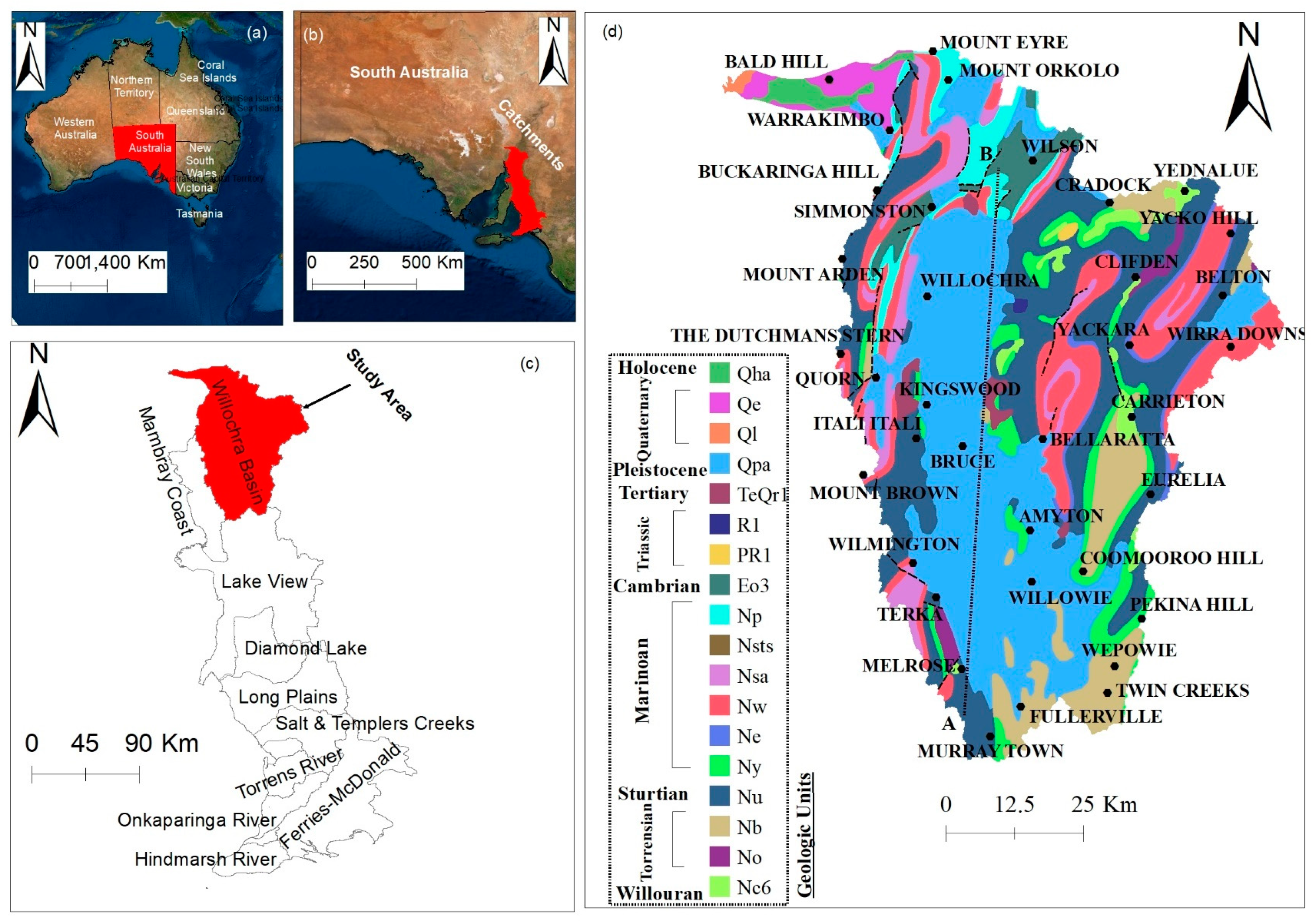
The main objective of this study is to highlight the importance of the integration of Remote Sensing (RS), Geographic Information System (GIS), and modelling as an efficient and low-cost approach to delineate recharge potential zonation, using the Willochra Basin of South Australia as an example (Figure 1). The Willochra Basin exhibits severe drought characteristics despite having considerable annual rainfall. Along the basin, land use has changed from cropping and grazing rotation to irrigated horticulture, which has led to the construction of larger farm dams (>5 ML). The combined impacts of flood irrigation and farm dam development have added more pressure on the water resources. Therefore, the need for sustainable management of the groundwater resource is crucial.
The recharge potential in arid regions varies significantly in space and time due to the low and intermittent precipitation, and high annual temperature [9]. As a result, several geological, hydrological, and geophysical methods have been developed to identify the dynamics of recharge in such areas [10,11,12]. However, most of these methods are considered time consuming and costly for water resources management.
During the last two decades, significant attention has been given to cost-effective approaches for mapping the groundwater recharge potential zones [13,14,15]. One of the most effective approaches, which has been extensively used for the water resources management, is the integration of remote sensing (RS), a geographic information system (GIS), and multicriteria decision-making (MCDM) [3,11,12]. The availability of RS data has facilitated the assessment of prospective groundwater potential zones at both local and regional scales [4,16,17]. In addition, MCDM has been widely used to deal with complex decision problems [16,17,18,19,20]. In the assessment of water resource evaluation processes, MCDM has been employed to find a solution for absent and/or vague information, effectively manage and understand decisions, and improve the quality of judgments [15,21,22]. In general, MCDM analysis is considered an effective technique for assessment in groundwater potential mapping, especially in data-limited areas [21].
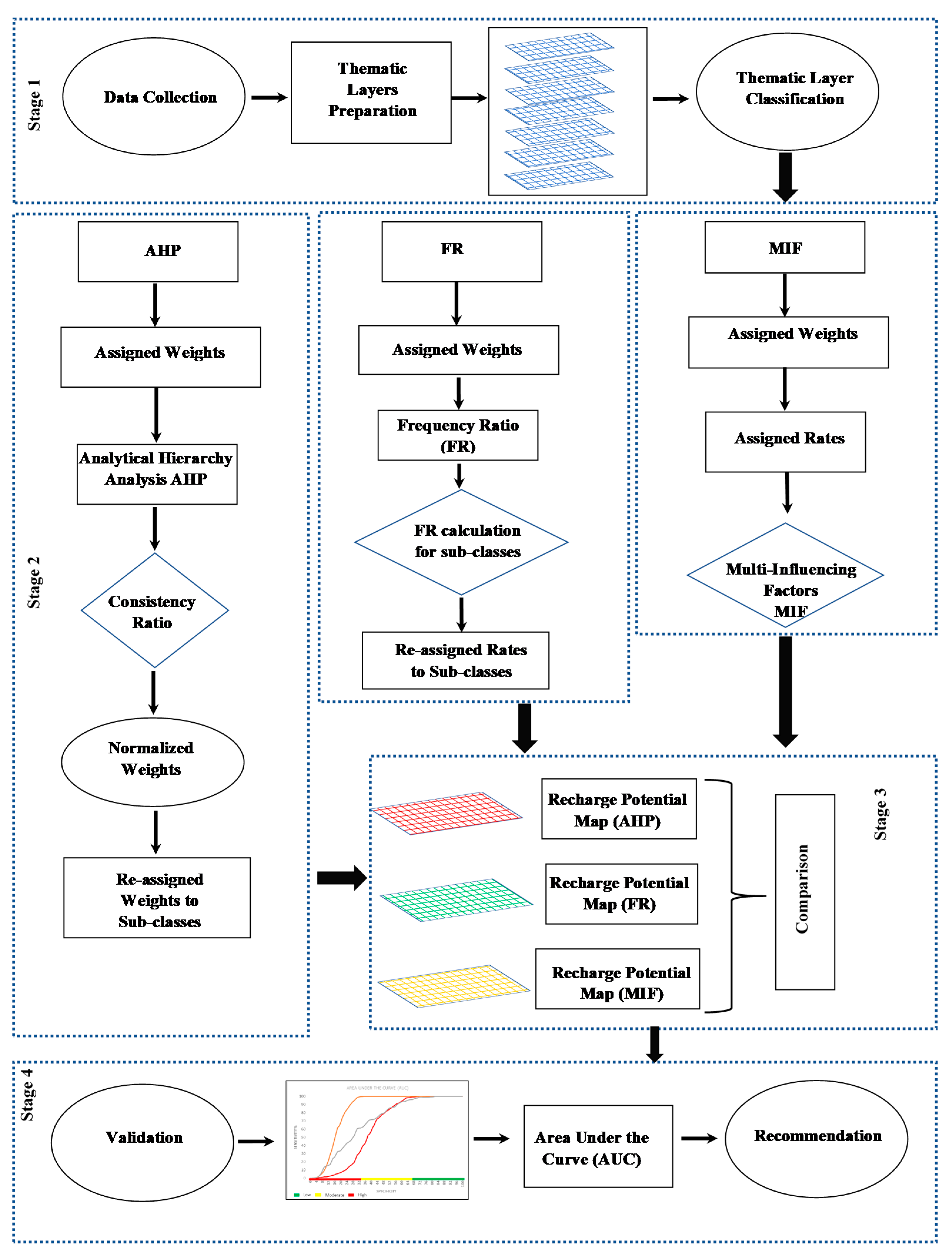
In this study, the analytic hierarchy process (AHP), the multi-influencing factor (MIF), and fraction ratio (FR) methods, such as MCDM, are applied to develop a sustainability assessment framework. These techniques have been recognised as powerful, efficient, and reliable methods for multi-criteria decision analysis in GIS environments [22,23,24]. AHP is a rational technique for organizing information alternatives based on a hierarchical framework by the application of mathematical pairwise comparisons [25]. It is a widely accepted model that can be employed for environmental management and hazard modelling purposes [5,6,7,8,26,27]. MIF is another elementary technique to execute MCDM based on existing knowledge of the relative importance of different factors [28,29,30,31]. It has been extensively used to delineate groundwater potential regions [32,33]. Additionally, the FR method has been integrated with other approaches to find out groundwater potential regions in many studies [21,34,35,36]. In recent years, several studies have been successfully undertaken to identify the recharge potential zones using advanced approaches such as statistical approaches [37,38], logistic model tree [39], artificial neural network [40], random forest, and maximum entropy models [41]. However, studies about the integration of the AHP, MIF, and FR methods, and RS and GIS to delineate groundwater potential zones are still few [36]. The present study is an attempt to incorporate a systematic integration of the three techniques with available remotely sensed and groundwater data to provide a rapid and cost-effective tool for delineating the groundwater potential zones.
The study aims to: (1) Develop, delineate, and integrate thematic layers for potential groundwater recharge zones, (2) compare the performance of MIF, AHP, and FR, and (3) validate the resulted potential groundwater recharge zone maps with the receiver operating characteristic (ROC) curve and available water data.

2. Study Area

The Willochra Basin is a local-scale groundwater resource in the Southern Flinders Ranges, South Australia, which is described as a non-prescribed region under the South Australian Natural Resources Management Act 2004. The basin is situated about 250 km north of Adelaide. The topography of the basin contrasts significantly from 965 m at Mt Brown in the southwest to 70 m near Lake Torrens in the northwest. The basin is bounded on high topographic features such as Mt. Robert, Mt. Eyre, and Mt. Arden (Figure 1). Many townships such as Melrose, Murray Town, Wilmington, and Quorn are distributed across the basin.
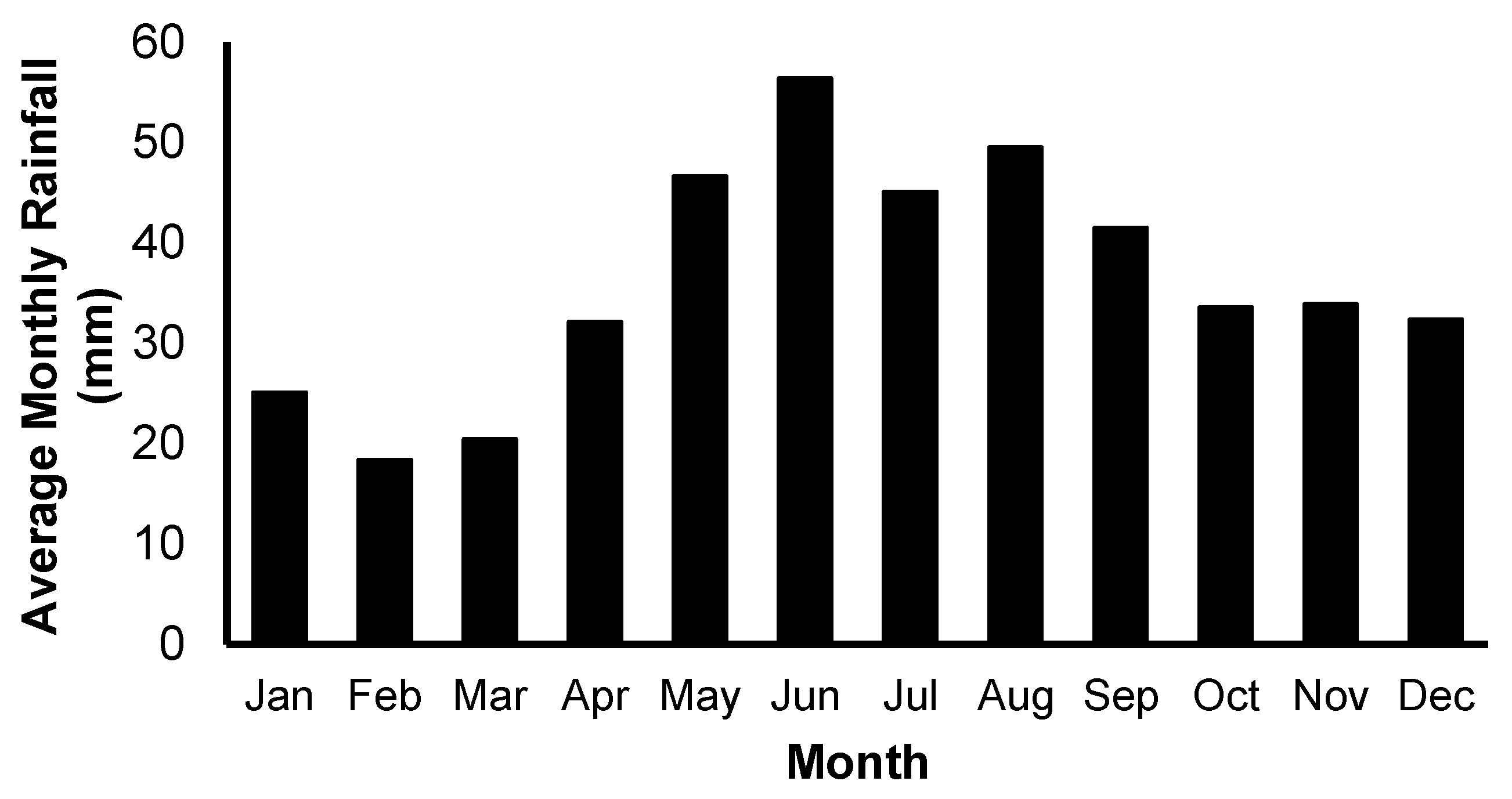
The climate of the study area is semi-arid with hot, dry summers, and cold, wet winters. The highest recorded rainfall (Figure 2) is observed in June and July and August and September (winter and spring). The lowest rainfall values are recorded in January, February, and March (Summer and Autumn). According to Reference [42], the average annual rainfall shows a significant increase from the southwestern areas (650 mm) to the northern areas (250 mm). In contrast, the potential annual evaporation varies from 2600 mm in the north to 2400 mm in the south of the basin.

3. Geology and Hydrogeology

The Willochra Basin is an intermountain (between ranges) basin located approximately 300 km north of Adelaide. The basin covers an area of 1165 km2, being 80 km in length and has a maximum width of 25 km. Geologically, Willochra basin consists of a sediment-filled series of bedrock depressions between Murray town in the south and Mount Eyre in the north. It is stretching in a north–south orientation and bounding by late Proterozoic and Cambrian rocks of the Adelaide Geosyncline [44]. The geosyncline consists of a thick sedimentary succession that extends as a continuous fold belt trending north–south, from Kangaroo Island in the south towards the north and north-east. It formed initially from undeformed sediments with a total thickness of over 12 km resulting from ongoing deposition in Neoproterozoic to lower Cambrian [44]. The deposition followed by a continuous rifting during the Delamerian Orogeny [45,46]. As a result of the Delamerian Orogeny, a number of tectonic domains, included from north to south: North Flinders Zone, Central Flinders Zone, Nackara Arc, Fleurieu Arc, and the Torrens Hinge Zone, were formed [44]. Each of these domains has their own particular deformation history, tectonic styles, and stratigraphy.
Within the basin, the Cainozoic sediments overlie the Delamerian Fold Thrust Belt, a north–south arcuate tectonogene formed during a major Cambro-Ordovician Orogeny [47]. The geologic succession consists of Cambrian limestone and Pound Quartzites, spreading downwards to Sturtian Tillite and Torrensian slates [48]. On the western fringes of the basin, the outcropped rocks are dominated by the hard rocks of the Ryanie Sandstone, Angepina Formation, Wilmington Formation, and ABC Range Quartzite. To the east, rock types become more fine and are dominated by the Saddleworth Formation, Auburn Dolomite, Appila Tillite, Tarcowie Siltstone, Tapley Hill Formation, Brachina Formation, and Cradock Quartzite [44].
The major structural features encountered in the study area are E–NE and N–NW trending folding, and the linear structural features associated with it [48,49,50]. The heterogeneity of the bedrock, and/or regional tectonic, structural and stress variations suggests that there may be a local variation in lineament orientations, length and density, throughout the study area [49,50,51].
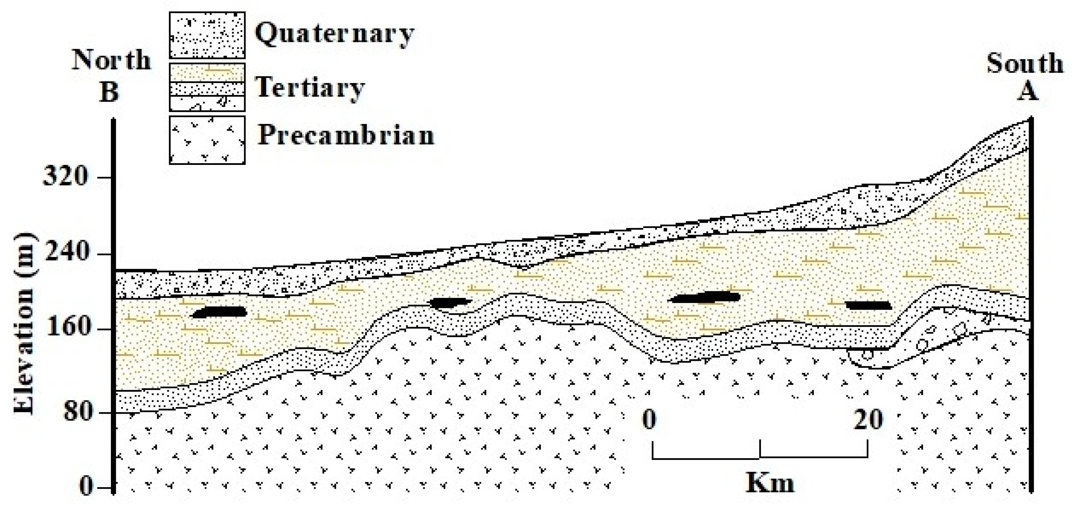
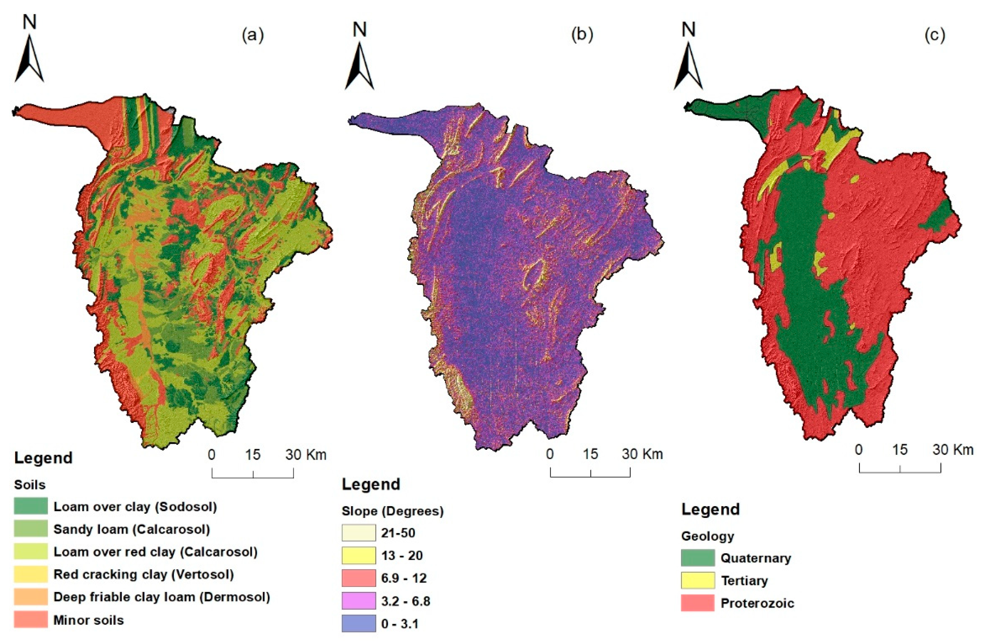
Hydrogeologically, three major aquifers are dominant (Figure 3): (1) The Quaternary sediments consist mainly of interbedded clays, sand, and gravel beds, particularly near drainage lines, and form unconfined aquifer that indirectly recharge the deep Tertiary confined aquifer [48]. The maximum thickness of Quaternary sediments is estimated at 90 m. Salinity of the aquifer is variable throughout the basin, signifying that local recharge and flow influences are important. Recharge is mainly from the south and south-west and from runoff of creeks and upward leakage from the underlying Tertiary aquifer, particularly in the north [48]. All over the basin, the Quaternary aquifer provides stock quality groundwater, with small areas having groundwater of suitable quality for irrigation. The best water quality is found to be in the vicinity of creeks where salinities are as low as 400 mg/L [42].
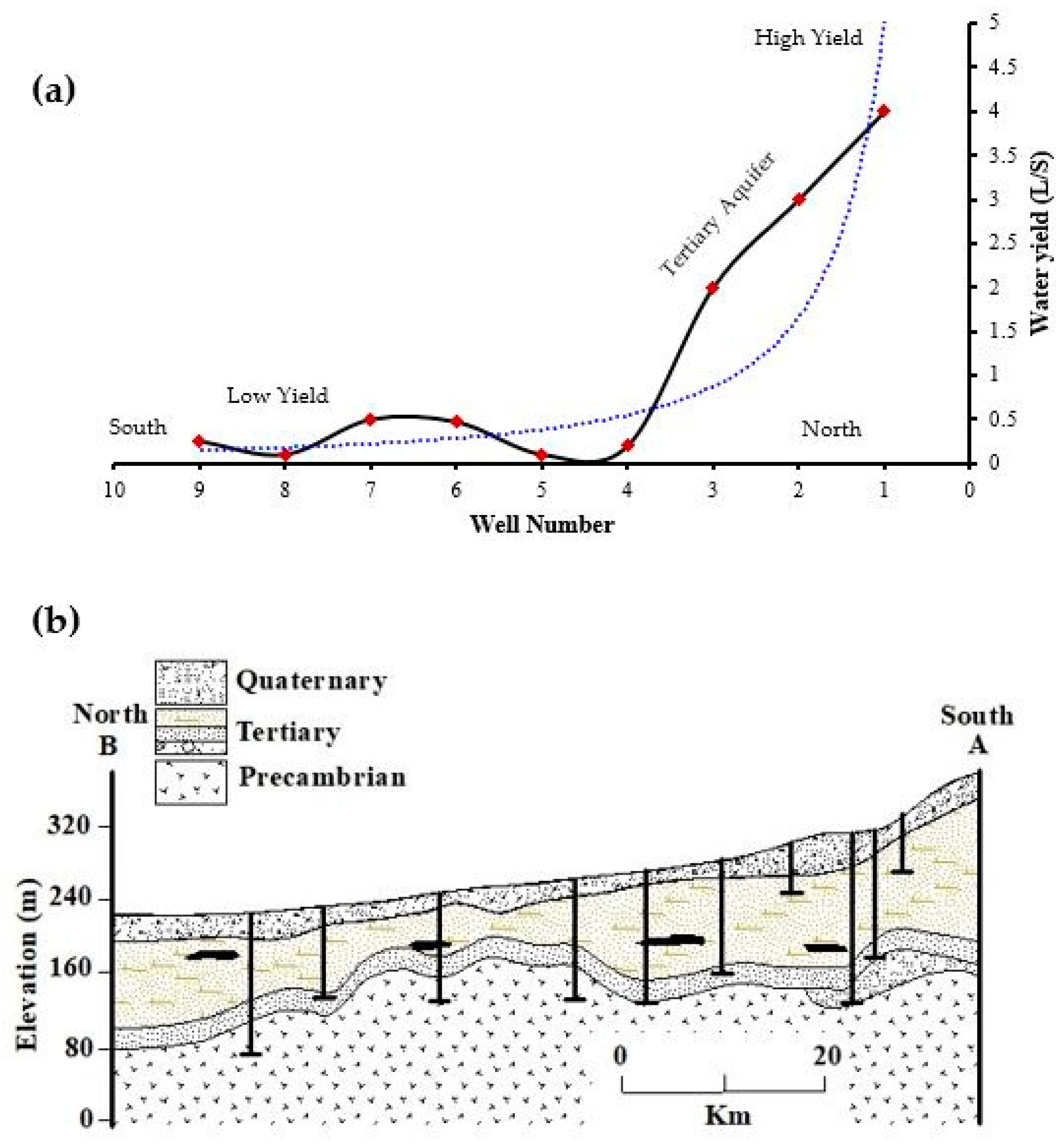
(2) Tertiary rocks are continuously outcropped over the basin, resulting in a confined aquifer with relatively fine-grained sand beds and maximum thickness ranging from 15 m in the south to 6 m in the north [42]. Groundwater flow in the Tertiary confined aquifer is mainly from the recharge areas in the south toward the north [42,52]. The aquifer is recharged by direct infiltration through outcrops in the high topographic ranges (Figure 4). This is supported by low salinity in areas proximity to these ranges. The water salinity is less than 1400 mg/L in the south, increasing gradually across the basin to greater than 7000 mg/L in the north.
(3) Fractured rocks are directly covered by Tertiary Sediments, indicating a direct hydraulic connection [42]. The water yield and volume of groundwater stored in the fractured rocks is unknown and was not given considerable attention. In addition, no recent investigation has been done to estimate sustainable yield of these aquifers.

4. Materials and Methods

4.1. Data Collection and Processing

In the present study, selection of factors is mainly based on the literature, data availability, characteristics of the study area, and their significance for the groundwater recharge potential zones [3,28]. This study used lithology, soil, slope, drainage, lineaments, land use, and rainfall as the seven significant factors affecting groundwater potential recharge.
Data were obtained from different websites and organizations to prepare the thematic layers required for mapping the groundwater recharge potential zones (Table 1). The Advanced Spaceborne Thermal Emission and Reflection Radiometer (ASTER, the Ministry of International Trade and Industry (MITI), Tokyo, Japan ) Global Digital Elevation Model (GDEM) Version 3 with 30 m and Landsat 8 OLI (Operational Land Imager) of 15 m resolution panchromatic band data were collected from the (https://earthexplorer.usgs.gov). While the rainfall, lithology and soil types, and water point data were collected from reliable secondary sources (http://waterconnect.gov.au) used for multi-criteria analysis (Table 1).
As shown in the flow chart (Figure 5), different methods were used in developing the thematic layers of the influencing factors. The watershed boundary was delineated using ArcGIS 10.7 software from the published toposheets of South Australia (1:250,000). The ASTER GDEM were then mosaicked and clipped to verify this boundary. By filling sinks of the DEM, the surface flow direction, flow accumulation, drainage patterns, and drainage density layers were extracted and calculated.
Landsat-8 OLI satellite data were used to extract lineaments and their density. In the present study, automatic extraction of lineaments, involving mosaicking and enhancement in ENVI TM 5.1, automatic extraction by edge detection, thresholding and curve extraction using the LINE module of PCI Geomatica, and exporting the lineament to GIS environment, was used. As line features could be humanmade constructions such as roads, the extracted lineaments were verified using the road network published by the Department of Planning, Transport and Infrastructure, South Australia.
In addition, the Landsat 8 satellite images were used to map the land use of the study area. Land use classification was performed using the maximum likelihood supervised classification method using a composite of bands 2, 3 and 4 of the Landsat 8 OLI data. Land use classes were obtained and verified using the Australian Land Use and Management Classification Version 8, which was derived from aerial imagery and on-ground field surveys, and available from the South Australian Government Data Web Directory. Pixel-based average annual rainfall data for 30 years was collected from the Bureau of Meteorology Australia, and the rainfall map is prepared by the Inverse Distance Weightage (IDW) interpolation technique in ArcGIS. IDW is commonly used as an accurate, time and cost-effective interpolation method which can be applied in limited measured data for specific purposes [53,54]. In this method, each estimated value is a weighted average of the surrounding sample points. Then, final weights are obtained as the inverse of the distance from an observer’s location to the location of the point being estimated. Lithology, soil, and well data were obtained from the South Australian government website (https://data.environment.sa.gov.au) and clipped in ArcGIS software to prepare thematic layers of the study area. All the layers, including delineated watershed, were resampled using the nearest neighbourhood technique and converted into cell size (30 × 30 m).

4.2. Multi-Criteria Decision-Making

In the present study, MIF, AHP, and FR techniques were used and compared to evaluate their efficiency in the identification of groundwater potential areas.

4.2.1. Multi-Influencing Factor

The multi-influencing factor technique involves the identification of the influencing criteria, establishing the interrelationship between the factors and assigning ranks to the factors [3,28]. Assigning ranks to the factors is based on author’s expertise, as in the published literature. In the present study, we use multi-influencing factor to evaluate seven influencing factors and to generate groundwater recharge potential maps. To ensure uniformity, the influencing factors were processed and scored to sub-classes within the factor map. Factors having significant influence were marked as major effect and were assigned a weight of 1.0, whereas minor influence was marked as a minor effect with a weight of 0.5, as shown in Figure 6 and Table 2.
The cumulative weights of major (EA) and minor effects (EB) are taken as the comparative rate. Subsequently, the score of each influencing factor is estimated using Equation (1):
S i = [ ( E e + E m ) i S i i = 1 n ( E e + E m ) i ]
where, Si is the proposed score, Ee is major influencing factor, and Em is minor influencing factor. For these factors, the weight was calculated, divided equally, and assigned a rank to each sub-class in each factor.
The resulting map was created through a raster calculation using Equation (2):
GRPZ = i = 0 n ( S i × R i )
where, GRPZ is the groundwater recharge potential zone, S i is the assigned weight of each factor, and R i is rank of each class, such as lineament density, lithology, soil, drainage density, slope, land use, and rainfall.

4.2.2. Analytical Hierarchy Process

The GIS-based AHP technique has been progressed by the worldwide academic network as an integral asset for investigating complex spatial choice issues [55]. In order to delineate potential recharge zones in the study area, the AHP technique was implemented in four steps: (1) selection of the influential factors on groundwater recharge zones, (2) creation of pairwise comparison matrix and estimation of relative weights, (3) assessment of matrix consistency, and (4) conduct of weighted overlay analysis [56,57]. In the first step, the importance of the factors that influence the groundwater recharge potential was evaluated based on a nine-point scale. Each factor was assigned rank on a scale of one (equal importance) to nine (extreme importance) [25] (Table 3). Secondly, in the pairwise comparison matrix, analysis was employed based on the input factors used for delineation of groundwater recharge potential zones. The AHP technique uses eigenvector and eigenvalue to avoid bias/subjectivity in the data by eliminating features that have a strong correlation between them.
The eigenvector was computed to show relative weights of each of the parameters towards recharge, while eigenvalues were employed to rank the importance of parameters to recharge. The sum of eigenvalues, called principal eigenvalue (λmax), is a measure of matrix deviation from consistency [58,59]. A pairwise comparison matrix is consistent only if the principal eigenvalue (λmax) is greater than or equal to the number of the parameters investigated (n), otherwise a new matrix is required. In the third step, the consistency index (CI) and the consistency ratio (CR) are calculated for verification. Inconsistencies of pairwise comparisons increase with increasing number of comparisons, [25,60], therefore, the consistency index (CI) measures the deviation or degree of consistency using Equation (3):
CI =   λ max n n 1
where, λmax = maximum eigenvalue for the pairwise comparison matrix, and n = number of classes.
The CI computation was followed by the consistency ratio (CR) calculation, a measure of the consistency of the pairwise comparison matrix using the following Equation (4):
CR =   CI RI
where, RI = ratio index. As the rule of thumb, the CR must be less than 0.05 in a 3 × 3 matrix, 0.09 in a 4 × 4 matrix, and smaller than or equal to 0.1 in a larger matrix to accept inconsistency (Table 4). If CR is greater than these, the subjective judgment would need to be revised.
Finally, Weighted Overlay Analysis is a common technique to create an integrated analysis, based on a pairwise comparison matrix of AHP [58]. In the present study, thematic layers of the different factors were reclassified, weighted, overlaid, and integrated in the Weighted Overlay Analysis tool in GIS to produce the final groundwater recharge potential zones (GRPZ), and Equation (5) is applied:
GRPZ =   w = 1 m i = 1 n ( w j ×   x i )
where, x i = normalised weight of the i-th class of factor, w j = normalised weight of the j-th factor, m = total number of factors, and n = total number of classes in a factor.

4.2.3. Frequency Ratio (FR)

The FR was calculated as the ratio between number of observational water wells and the factors that influence groundwater recharge potential. For a certain factor, FR can be expressed following Equation (6):
FR = ( P gw T gw P f T f ) = ( %   Wells %   Pixels )
where, P gw is the number of pixels with wells for each factor, T gw is the total number of wells, P f is the number of pixels in the classes of a factor, and T f is the total number of pixels of a factor. Then, all the factors with their FRs were integrated and summed to map the groundwater recharge potential zones using Equation (7):
GRPZ = i = 1 n FR i
where, GRPZ is groundwater recharge potential zone, and FR i is FR of each factor.

4.3. Cross-Validation Technique

In this study, the accuracy of the MIF, AHP, and FR methods in delineating groundwater recharge potential was verified by implementing the values of the area under the curve (AUC) of the ROCs (Receiver Operating Characteristics) and water data along the geologic section. The area under the curve is applied as a forecast model quality to evaluate the capability of a model to correctly predict the occurrence or non-occurrence of pre-defined events [60]. Therefore, groundwater recharge potential maps were validated using 2842 existing wells in Willochra basin. Rate curves were generated by dividing the groundwater potential map into 100 classes with accumulated 1% intervals. The graph was plotted using cumulative percentage of potential maps called “specificity” (on the x axis) against the cumulative percentage of groundwater occurrence known as “sensitivity” (on the y axis). The predictive performance was based on the AUCs and classified as either acceptable (AUCs = 0.7–0.8), excellent (AUCs = 0.8–0.9), or outstanding (AUCs > 0.9) [61].
The resultant GWPZ map was further validated using the observed well-yields of water wells obtained from the Department for Environment and Water, South Australia. The water wells were chosen along the geologic cross-section and were referred to as high, medium, and low water yield. This well data was used as a reference point to recognize the groundwater recharge potential map accuracy.

5. Results and Discussion

5.1. Selection of Factors Influencing GPZ

In order to identify recharge potential zones in the study area, thematic layers of the controlling factors were used. As mentioned above, the seven thematic layers include lithology, slope, drainage density, lineament density, land use, and soil type.

5.1.1. Lithology

Lithology controls the recharge and storage of the rock aquifers through the porosity and permeability that control the ability of the rocks to transmit water and the rate at which groundwater flows [33]. Figure 7 shows the resultant lithological thematic map layer generated from geologic map and verified by the Landsat images. The lithology of the study area consists of the sandy clays, interbedded with hard marly limestone of Quaternary (8%), clay intercalated with fine sandy clay, silt clayey sand of Tertiary (32%), and Phyllites and slates of the Proterozoic (60%).

5.1.2. Slope Features

Slope features play a major role in groundwater availability and its distribution [62]. In Figure 7, the slope map of the study area was extracted from ASTER GDEM using the slope tool in ArcGIS. It was created using the eight-node operation of the slope tool which calculates the change in elevation at a point using elevations of the surrounding eight neighbours. Within the study area, five classes of slope were initially identified, flat (0–3.1°), gentle (3.2–6.8°), moderate (6.9–12°), steep (13–20°), and very steep (21–50°). Generally, the study area has a moderate slope (20.54%) to gentle (18.43%).

5.1.3. Soil Type

Soil texture plays an important role in the infiltration of water, and therefore influences the groundwater recharge potential of groundwater [36,57]. The soil map of the study area in (Figure 7) shows six soil types namely, loam over clay (Dermosol/Sodosol), calcareous loam (Lithocalcic Calcarosol on clay), sandy loam, red cracking clay (Vertosol), and deep friable clay loam (Dermosol), and other minor soils, constituting about 35%, 20%, 14%, 11%, and 8%, respectively.

5.1.4. Drainage Density

Drainage features is another geomorphic measure of groundwater recharge potentiality [63]. A drainage network can be expressed as drainage density, indicating the total length of streams relative to an area (km/km²). Using the line density tool of the spatial analyst toolbox in ArcGIS software, a drainage density map of the study was produced. Five drainage density categories were identified (Figure 8a), namely, very high (2.7–3.4 km/km2), high (2.5–2.7 km/km2), moderate (2.1–2.5 km/km2), low (1.5–2.1 km/km2), and very low (0.3–1.6 km/km2). The drainage density in Willochra basin is mostly very high (32%) to high (40%), causing less infiltration and high runoff. Thus, a drainage density of the basin has an inverse function of permeability; thus, lower drainage density indicates a highly permeable rock, high infiltration, and less surface runoff, while higher drainage density indicates low permeability, less infiltration, and more runoff [22,64].

5.1.5. Land Use

In arid regions, land use changes may modify recharge volume, timing, and amount, and affect groundwater resources [65,66,67]. It has been found that negative land use change and land cover alteration processes such as cropping and settlement could decline the recharge potential zone, while positive land use change and land cover alteration processes such as dense forest and degraded forest could help with sustaining the recharge potentiality [67]. Across the study area, six primary land uses were identified (Figure 8b), dryland agriculture (56%), water (16%), irrigated agriculture and plantations (10%), natural environment (5%), conservation environment (5%), and intensive uses (4%). Dense agriculture areas have high potentiality to recharge and store groundwater, whereas exposed bare rock and built-up areas are less suitable for infiltration and recharge.

5.1.6. Lineament Density

Lineaments on the earth’s surface, such as faults, joints, fractures, and fold axes, are commonly used parameters for identifying groundwater recharge potential zones [68,69,70]. In the present study, lineaments from geologic and topographic maps and Landsat images were demarcated to calculate lineament density. The density of lineaments is defined as the cumulative length of lineaments per unit area. Based on the lineament density map, five main categories were identified (Figure 8c), very low (0–018 km/km2), low (0.8–1.13 km/km2), moderate (1.14–1.45 km/km2), high (1.46–1.83 km/km2), and very high (1.84–3 km/km2). Nearly 50% of the study area is covered by low to moderate lineament density.

5.1.7. Rainfall

Rainfall is identified as the major source for recharging groundwater to aquifers and the main driver of the entire hydrologic regime [71]. The mean annual precipitation from six stations distributed across the Willochra Basin was used to prepare the rainfall map (Figure 8d). The resulting rainfall shows five major classes of rainfall, the majority of the area is in moderate condition (36%), whereas there is adequate rainfall to the south-western regions.

5.2. Qualitative Classification of Defined Factors

In order to assign weight for the controlling factors, thematic layers were reclassified according to the relative influence on groundwater recharge. Based on their natural breaks, each layer was reclassified into three classes, high, moderate, and low groundwater recharge potential.

5.2.1. Lithology

Lithology is an important factor that controls recharge through the influence on the nature of rocks, drainage density, and drainage gradient. In this study, Quaternary sediments were classified as moderate groundwater recharge potential because of the unconfined nature of the clay and sand interbeds of low permeability (Figure 9a). The Quaternary sediments constitute the topmost layers in the stratigraphic sequence and outcropped at some parts within the basin. It is characterised by variable thickness and variable salinity (500–3500 Mg/L). In addition, a relatively low water yield (<3 L/s) indicates low transmissivity of the aquifer. The highest transmissivity sections of these aquifers are usually located where there are major bedrock structures or surface drainage (for the shallowest aquifers).
The Tertiary rocks were assigned high groundwater recharge potential values because of the confined nature, sandy facies, high water yield, and relatively continuous extension over the basin (Figure 9a). The recharge is mainly from the runoff generated near the flanks of ranges. While the aquifer thickness is variable through the basin, it ranges from about 15 m in the south to less than 6 m in the north. The Proterozoic rocks were assigned low groundwater recharge potential value due to low permeability and high topographic and steep slope setting. The relationship between rock permeability and runoff generation and drainage density has been emphasized in many studies [72]. Lithology influences the water-holding capacity of aquifer and directly affects the occurrence and distribution of groundwater [73].

5.2.2. Slope Features

Slope controls the response of terrains to runoff and infiltration [31]. The reclassified slope map was produced based on the groundwater recharge potential (Figure 9b). Within the study area, steep slope areas in undulating hilly areas were assigned low recharge values because steep slopes can result in greater soil erosion rates with a relatively quick runoff and low groundwater recharge potential [74]. Low slopes are considered as having high groundwater recharge potential as gentle slopes can permit more infiltration through the soil and ultimately recharge to the underlying aquifers [75]. The high recharge is concentrated in the southern and central regions where topography is relatively flat.

5.2.3. Soil Type

Soil characteristics are important prospects in delineating groundwater potential as they control the water holding capacity [76]. In this study, soil is reclassified depending on grain size, clay and silt content, texture, and infiltration capacity. The high recharge values were assigned for coarse-grained soils which have high sand content and little or no clay (Figure 9c). The fine-grained soils such as fine loamy soils were assigned moderate groundwater recharge potential values, while stony soils are considered as low groundwater recharge potential zones.

5.2.4. Drainage Density

Drainage density was reclassified into three classes (Figure 10a), higher groundwater recharge potential rank is assigned to 2.8–3.4 km/km2 and the least given to 0.5–2.6 km/km2. High drainage density indicates a high-water concentration and excessive runoff and is given higher weight in relation to recharge [29]. In contrast, in high topographic areas, the number of streams is less, and slope is relatively steep, therefore, areas with low drainage density are low in groundwater recharge potentiality.

5.2.5. Land Use

Land use has a major influence on the occurrence and development of groundwater in a terrain [77]. The occurrence of built-up and barren lands in an area has a negative impact on water infiltration due to sealed features that reduce permeability and increase runoff potentiality. In contrast, the distribution of surface water bodies facilitates the percolation because of the permanent occurrence of water at the surface [31]. Similarly, agricultural lands can allow more infiltration through the pore spaces of the soil, which can trap and hold the water in the roots and permit water to percolate into the rock and soil. Therefore, the land use map was reclassified by assigning agriculture and water bodies’ areas as good sites for groundwater recharge (Figure 10b), while settlements and barren lands are considered to have a poor groundwater recharge potential [30,78].

5.2.6. Lineament Density

Lineaments can act as conduits for groundwater flow, and hence, have good groundwater recharge potential [69]. The density of and proximity to lineaments and lineament intersections do have some influence or act as favourable sites for groundwater availability [79].
The lineament density map was reclassified based on the fact that lineaments improve secondary porosity and permeability of rocks. Accordingly, three classes are identified: high, moderate, and low lineament density. The higher lineament density (range, 1.47–2.98 km/km2) reflects a higher potential of groundwater, and lower lineament density (<0.98 km/km2) has low groundwater recharge potential. Figure 10c shows that the north-western and south-eastern parts have a relatively high lineament density, indicating more secondary porosity, and thus potential conduits for groundwater movement [80,81,82].

5.2.7. Rainfall

In arid regions, recharge is characterised by episodic, infrequent, and high-intensity rainfall events [9]. Duration and frequency of rainfall events can control the amount of groundwater recharge [3]. Rainfall in Willochra basin is reclassified into three classes according to their relation to the groundwater recharge potential (Figure 10d), the high rainfall (430–609 mm) is given a higher rank and considered favourable to recharge, and the lowest (224–324 mm) is assigned a lower groundwater recharge potential rank. In the study area, high precipitation is noticeable along southern areas and lower values are evident in the northern areas.

5.3. Recharge Potential Mapping

For identification of groundwater potential zones, three methods, AHP, MIF, and FR, were used. For each method, individual thematic layers were classified and ranked (Figure 11).

5.3.1. Multi-Influencing Factor

The MIF has been widely used to understand the factors impacting groundwater potential [3,28,62]. Based on the MIF method, the groundwater potential map for the study area was prepared. The groundwater recharge potential map using MIF reveals that 33% of the study area falls into high groundwater potential zones, distributed along the southern areas with relatively low drainage density, shallow sandy soils, Holocene deposits, and predominantly agricultural land use/land cover (Figure 11a). About 37% of areas are moderate potentiality, observed in central areas that are covered by loamy sand soils, and have moderate lineament and drainage densities, and moderate rainfall. Whereas the poor groundwater potential zones (29% of the study area) are mainly dominated by steep slopes and ridges, where the lithology is mostly compact and massive Proterozoic rocks (Figure 11a).
The generated output map shows a significant reflection of the main factors like slope and lithology in controlling the distribution of groundwater recharge potential zones. Southern and south-western parts of the study area have a high groundwater recharge potentiality due to the distribution of alluvial plains and agricultural lands with high infiltration ability. While northern and eastern parts of the study area characterize low groundwater recharge potential due to the low permeable rocks and steep slope features, which have less influence on water holding capacity and recharge capability.

5.3.2. Analytical Hierarchy Process

AHP is a very common technique extensively used for multi-criteria decision-making analysis in the last few decades [36,57]. To determine the groundwater recharge potential zones, a matrix of a pairwise comparison is developed for assigning weight values. Lithology is considered as the most influential parameter due to the nature of the geological formations and how they influence infiltration rates in the surficial materials [62]. In construction of the pairwise comparison matrix (Table 5 and Table 6), selection and weighting the different factors was dependent on the lithology as an essential controlling factor for the occurrence and distribution of groundwater in any drainage basin [83]. It is essential for slope and soil development. Slope values reflect a difference in elevation resulting from weathering of rocks, therefore the lithology–slope pair was assigned a weight of 3. In addition, soil type, texture, and thickness are directly related to both lithology and slope, as well as erosion and deposition, therefore the lithology–soil type pair was assigned a weight of 6.
The ranking analysis in AHP techniques is necessary for the determination of the high and the low weight. The eigenvalues and principal eigenvalue (λmax) were calculated to rank the importance of the factors related to recharge (Table 6 and Table 7). In the present study, the principal eigenvalue of 7.56 was achieved and used for the calculation of consistency ratio. The threshold value of the consistency ratio (CR) was found to be 0.09, which means the judgments matrix is reasonably consistent and acceptable for the overlay analysis.
The resultant map from AHP analysis confirmed that high groundwater recharge potential zones (33% of the study area) are dominant, with coarse sandy lithologies, high rainfall, sandy soil, and high lineament densities in the southern and western areas (Figure 11b). Moderate groundwater potential zones (34% of the study area) are obvious in the central and eastern areas due to the distribution of alluvial deposits, moderately weathered pediplains, moderate lineament densities, and agricultural land use. The poor groundwater potential zones (33% of the study area) are in the eastern and northern areas, which are covered by hilly terrain features, impermeable Proterozoic, and steep slopes.

5.3.3. Frequency Ratio

The FR is the ratio between the percentage of available wells under a certain class and the percentage of area falling under the class of a factor [21]. Lower FR values (<1) indicate a weak correlation, while a higher FR values (> or = 1) reflect a good correlation. In the present study, the FR values were generally >1, indicating a high correlation (Table 8). The groundwater recharge potential mapped using the FR model indicates that 38% of the basin area has high potential and 30% has moderate potential for groundwater recharge. The rest of the area (32%) has low groundwater potential (Figure 11c). According to the observed relationships between groundwater well locations (with yield values ≥0.01 L/s) and each controlling factor, groundwater recharge potentials are higher where there is higher rainfall. Thus, high rainfall leads to high infiltration and good recharge of the groundwater aquifers. The relationship between groundwater occurrence and rainfall suggests that the southern areas that receive higher mean annual rainfall (430–609 mm) have higher groundwater potential.
In the case of slope, the FR is high (1.08) for the gentle slope classes, indicating a high correlation between slope features and the groundwater recharge potential (Table 8). However, FR increases with decrease in slope, suggesting low recharge probability. To understand this, it is important to relate slope with other controlling factors such as lithology and soil. The extension of slope classes is spatially correlated with the extension of lithologies in the southern and western areas (1.38). These lithologies consist mainly of coarse sand and gravel which probably have higher hydraulic conductivity and good permeability. The higher FR (1.94) of the shallow sandy soils that are dominant in the same areas supports this conclusion.
Considering other factors such as drainage density and lineament density, it is evident that areas with low drainage density and high lineament density have higher FRs and are favourable for groundwater recharge potential. Another important observation is that areas of agricultural land use reflect a high probability of groundwater recharge potential and have a high FR (1.03).

5.4. Multi-Criteria Decision-Making

In recent years, many methods have been implemented to delineate the groundwater recharge potential zones, however, comparison among influencing factor, frequency ratio, and analytical hierarchy process techniques confirmed a good proficiency in delineating the groundwater recharge potential zones [36]. Results from the three techniques indicate that lithology, rainfall, soil, and lineament density are the major factors that influence groundwater potential (Table 9). These findings agree with References [28,62], who applied similar rankings and gave the highest weights to these same factors. In all three models (IF, AHP, and FR), the final maps show that the southern and western areas of the Willochra basin are promising areas for groundwater recharge potential (Figure 11). However, the areal distribution is different between models for the different classes. For example, the AHP and MIF techniques showed relatively low groundwater recharge potential area compared to the FR method. These results agreed with several studies who recommended it as a more effective and reliable approach for groundwater recharge potential mapping [21,36]. They claimed that the level of accuracy in the FR technique depends on statistical approaches rather than on user-based/subjective rankings used in the MIF and AHP techniques.

5.5. Cross-Validation with AUC and Well Data

Checking and validating the accuracy of any applied model is an essential practice to evaluate the accuracy of results. Several methods are widely used to validate groundwater potential maps. Abdalla [84] integrated RS and GIS to delineate groundwater potential regions in the Central Eastern Desert, Egypt. He used available well data to validate the groundwater recharge potential map and revealed that most water points were located within the identified good to moderate potential areas. In addition, AHP and GIS were used to map groundwater potential zones in southern Iraq [85]. The groundwater recharge potential map was validated using the abstraction rate of wells and found a prediction accuracy of 72%.
Also, the MIF and RS are integrated in GIS to delineate groundwater recharge potential zones in Eastern Desert of Egypt [28]. The output groundwater recharge potential map was verified using a geophysical approach, revealing the agreement between the identified good recharge zones and the groundwater occurrence. Moreover, Rahmati et al. [55] validated the results of an integrated AHP, GIS, and RS technique for mapping the groundwater potential in the Kurdistan region of Iran using the ROC.
In the validation of the present study, water well data is analysed with resultant groundwater potential maps obtained from MIF, AHP, and FR (Figure 12). The region below the ROC curve is between 0 and 1. A larger area under the ROC curve refers to the higher efficiency of spatial modelling models, such as groundwater mapping potential. Generally, a good model has an AUC value of 0.7–0.9, while an excellent model has values over 0.9. The findings of the ROC analysis indicate that area under the curve (AUC) was of 62%, 70%, and 84% for MIF, AHP, and FR, respectively. The approach adopted in this research can, therefore, be assumed to be accurate and consistent in predicting groundwater recharge potential. This confirmed that the FR model is an effective tool in the assessment of groundwater recharge potential mapping when sufficient yield data are available [21,36].
The validation results increase confidence in the applied methodology. The water yield of available wells along a north–south geological cross-section was used for further validation of results (Figure 13). Nine water wells across the basin representing distribution of hydraulic head in relation to topography and geology in the various recharge potential zones are presented. The results show a good agreement with the identified groundwater recharge potential classes. It is clear that the groundwater recharge potential zones coincide with the available well data. High water yield defines areas where the recharge is high infiltration in relation to hydraulic loading. This is consistent with the largest recharge occurring in the southern regions and gradually decreasing towards the middle part with moderate recharge potential. The zones are clearly controlled by the lithology, depth to water, and structure, where high water yield corresponds to areas of Tertiary rocks (Figure 13a). The Tertiary aquifer is well-known for high yielding (>4 L/s) and low salinity (<1000 mg/L) in the south-western areas. Within the basin, salinity varies considerably in the Tertiary confined aquifer, ranging from less than 1000 mg/L in the high recharge areas to more than 7000 mg/L [52]. The overall interpretations confirm the reliability of the groundwater potential maps; hence, the maps offer a useful guide for any further investigation.

6. Conclusions

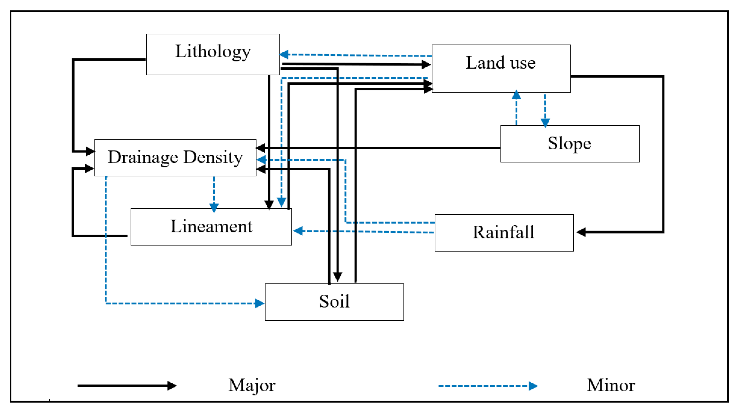
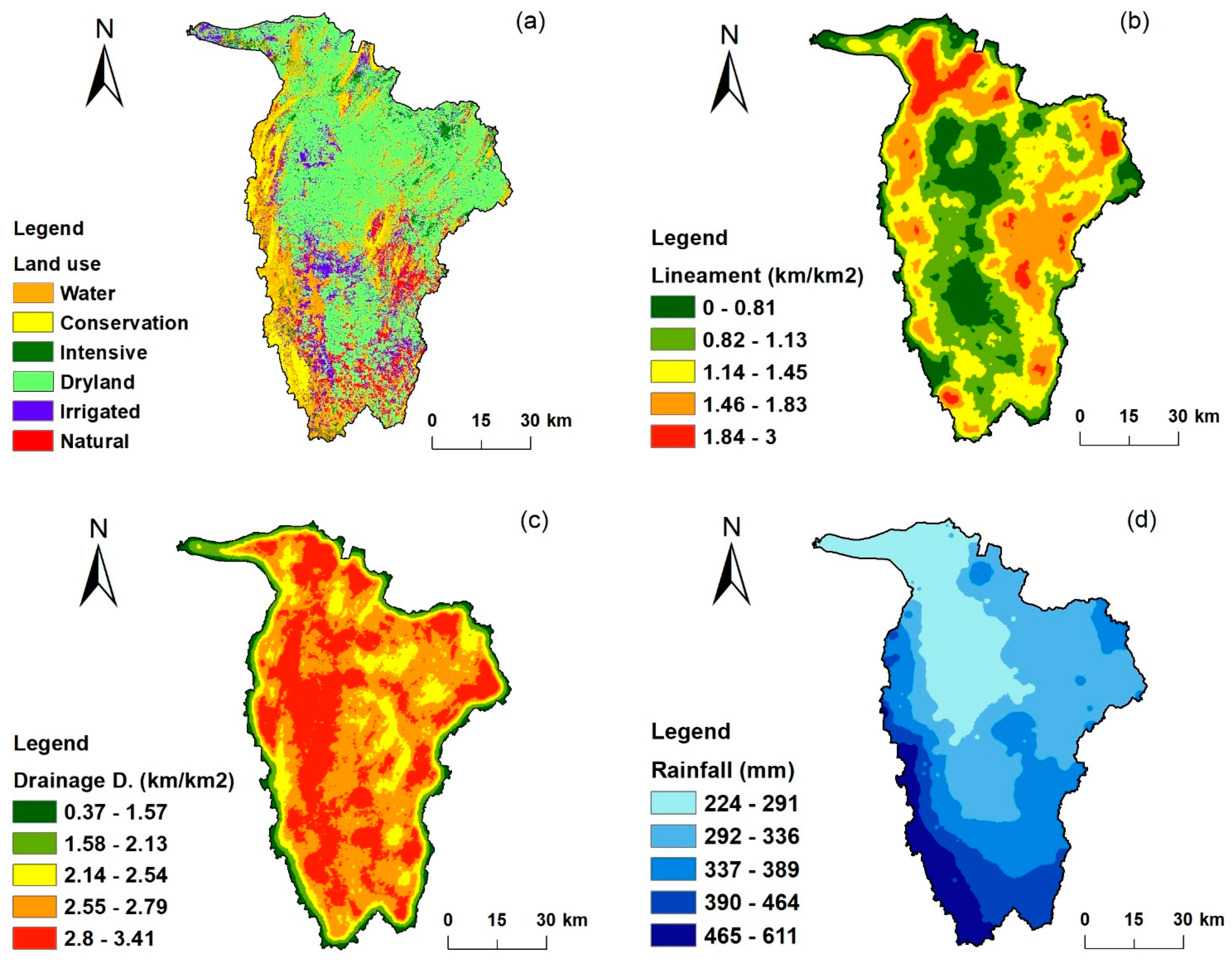
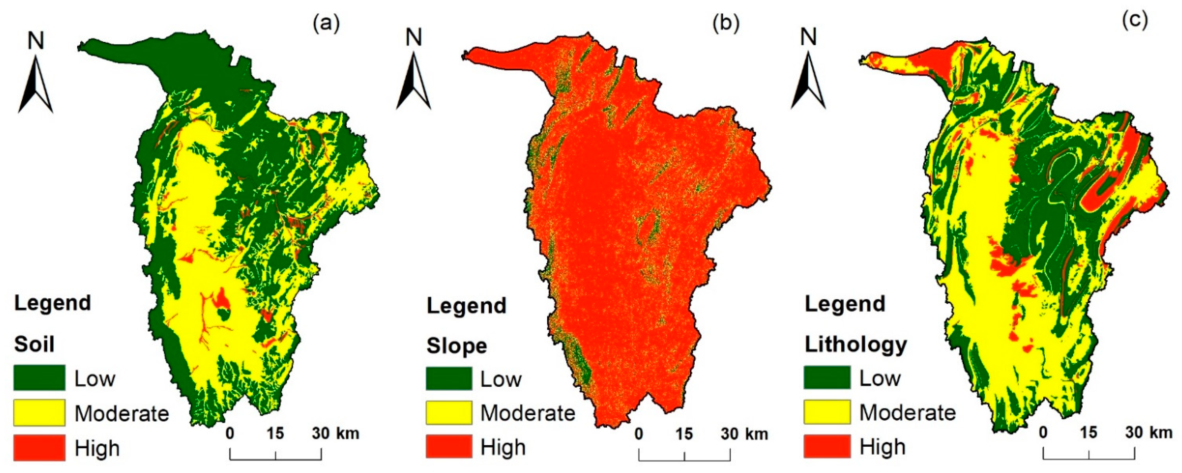
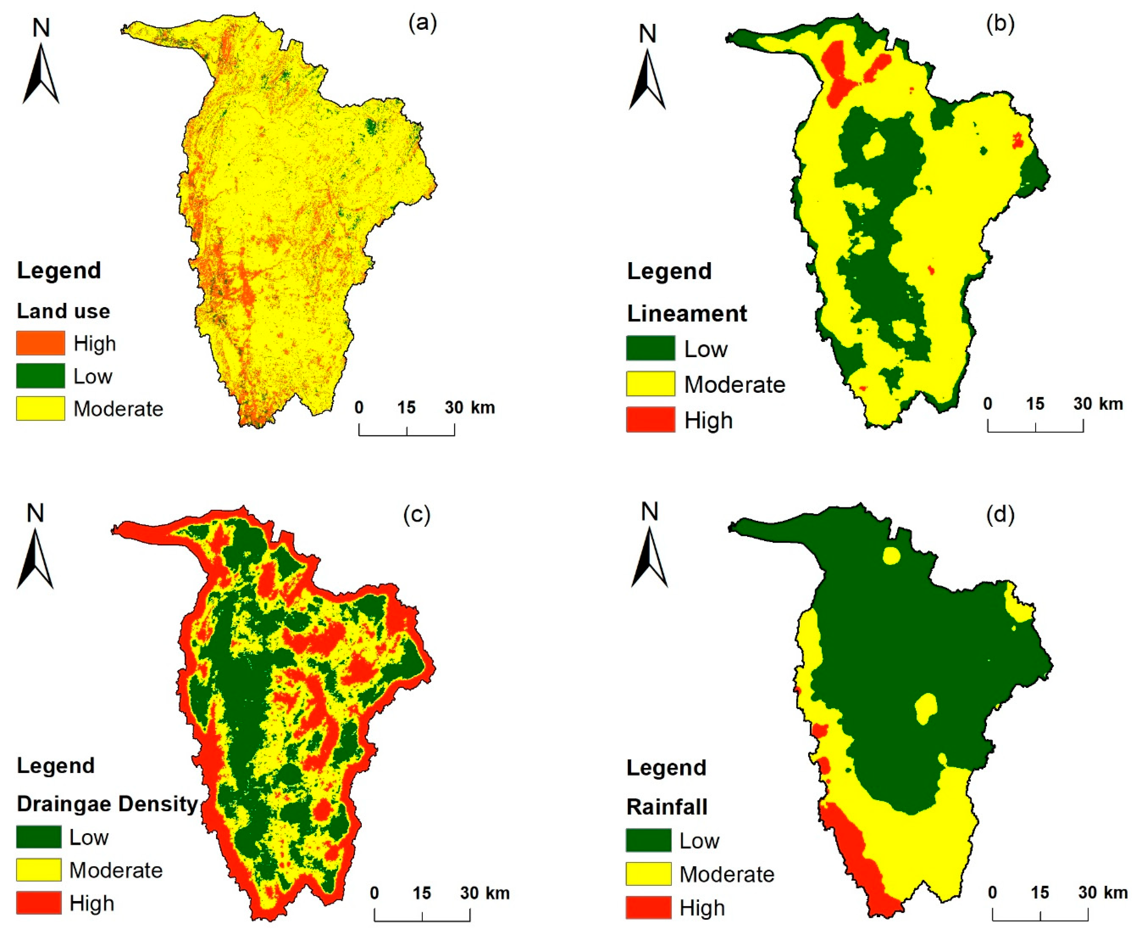
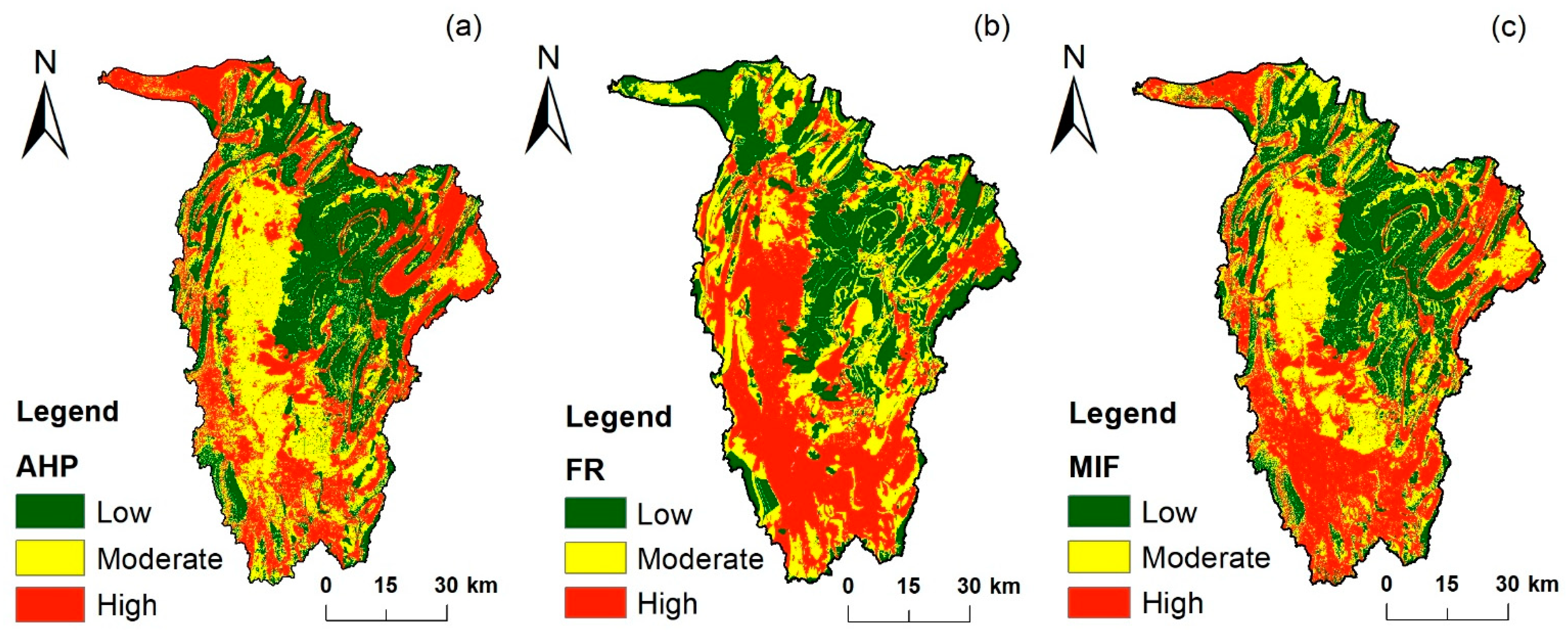
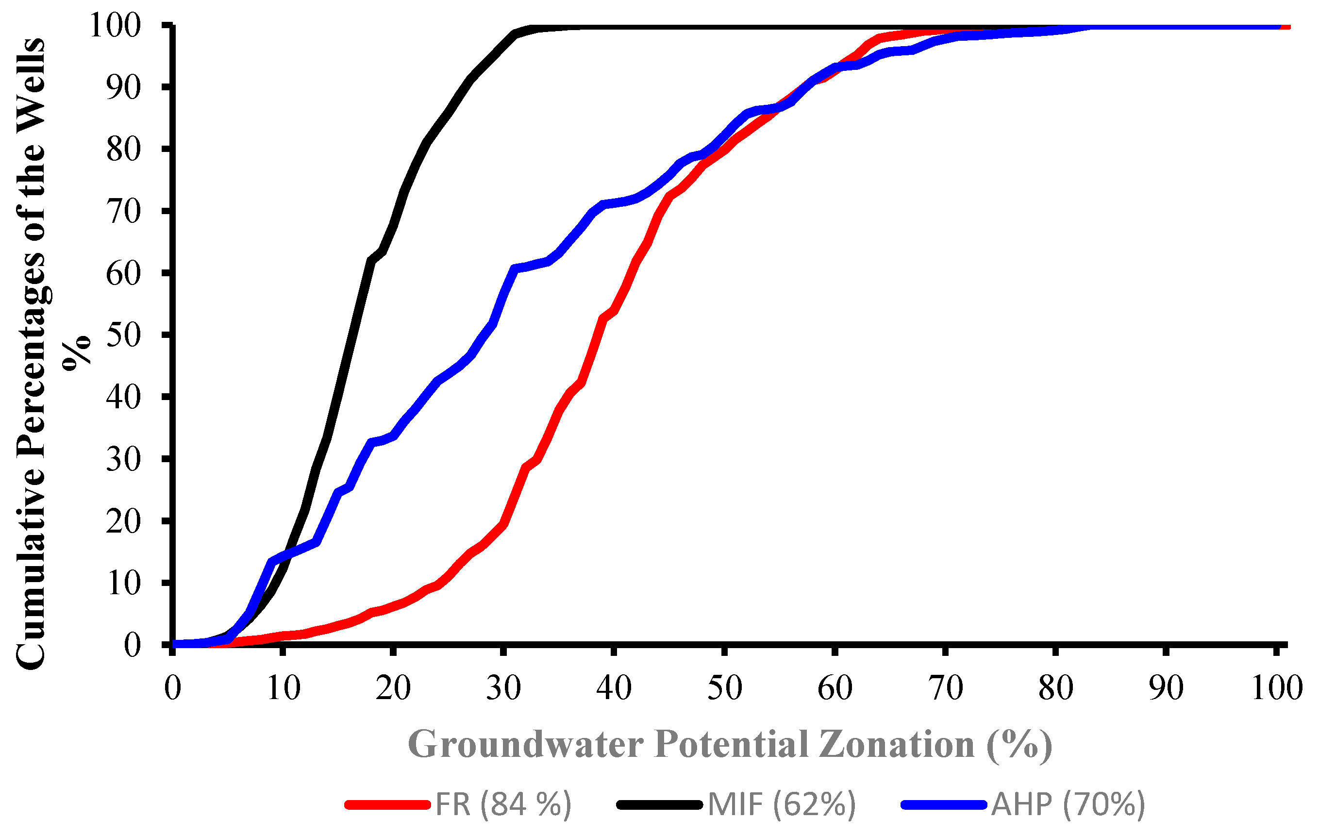
To sustain groundwater resources, delineation of the most favourable recharge zones is urgently needed. The integration of RS and GIS, along with the MIF, AHP, and FR techniques, has been recognised as an efficient and powerful tool for mapping and identification of groundwater recharge potential zones. The main objective of this study was to evaluate the applicability of MIF, AHP, FR, GIS, and RS techniques to map groundwater potential. The groundwater recharge potential of a region depends on the direct and indirect influences of several factors. In the present study, seven thematic layers representing the main influencing factors including (lithology, slope, drainage density, land use, lineament density, rainfall, and soil) were integrated together using GIS to generate groundwater recharge potential maps for the Willochra Basin, South Australia. According to the final output map, the study area could be classified into three distinct groundwater recharge potential zones, such as high, moderate, and low. Of the basin area, 33–38% was identified as high potential areas for groundwater recharge and correspond to the southern region of the area. Moderate groundwater potential zone covered an area of 30–37% and low groundwater recharge potential ranged from 29% to 33% of the study area. To check the accuracy of the resultant maps, the data were validated using the AUC and available well data along a hydrogeological cross-section. The AUC of the FR technique was high (84%), indicating that this method was highly accurate, and more accurate than the MIF and AHP techniques. Moreover, well data showed a good agreement with the findings from the mapping and AUC. This study proved that the multicriteria decision analysis can be effectively integrated with RS and GIS techniques for an accurate and cost-effective assessment of groundwater recharge potential. The methodology in this study can be straightforwardly applied for sustainable development and management of the precious water resources in other data-limited areas. The resultant maps could be used as a blueprint for any future groundwater assessment and management in Willochra Basin. The groundwater potential maps would help policymakers to formulate better decisions. In addition, it could support the decision-makers in the selection of appropriate locations for drilling wells based on demand.

7. Recommendations and Further Research

In order to have a sustainable development of groundwater resources in this area, further investigations are required, including the following:
  • A more detailed study of the high-potential recharge zones in the Willochra area is recommended to have a full understanding for the assumed measures of the mapping results.
  • A consultation of hydrology and hydrochemistry and soil experts is needed to validate the results about the suitable locations of the groundwater recharge.
  • A validation using a sensitivity model is recommended to evaluate the results of the study.

Author Contributions

Conceptualization, A.A. (Alaa Ahmed) and A.A. (Abdullah Alrajhi); methodology, A.A. (Alaa Ahmed), A.A. (Abdullah Alrajhi) and C.R.-A.; software, A.A. (Alaa Ahmed), C.R.-A.; validation, A.A. (Alaa Ahmed), A.A. (Abdullah Alrajhi) and C.R.-A. formal analysis, A.A. (Alaa Ahmed); writing—original draft preparation, A.A. (Alaa Ahmed), A.A. (Abdullah Alrajhi) and C.R.-A.; writing—review and editing, A.A. (Alaa Ahmed), A.A. (Abdullah Alrajhi) and G.H.; supervision, G.H., project administration, A.A. (Alaa Ahmed). All authors have read and agreed to the published version of the manuscript.

Funding

This research received no external funding.

Informed Consent Statement

Not applicable.

Data Availability Statement

Not applicable.

Acknowledgments

The authors would like to thank Abdullatif Lacina, University of South Australia, for help in editing, revising, and improving the manuscript.

Conflicts of Interest

The authors declare that they have no known competing financial interests or personal relationships that could have appeared to influence the work reported in this paper.

References

  1. Hamdy, A.; Ragab, R.; Scarascia-Mugnozza, E. Coping with water scarcity: Water saving and increasing water productivity. Irrig. Drain. 2003, 52, 3–20. [Google Scholar] [CrossRef]
  2. Rosegrant, M.W.; Cai, X. Global water demand and supply projections: Part 2. Results and prospects to 2025. Water Int. 2002, 27, 170–182. [Google Scholar] [CrossRef]
  3. Yeh, H.-F.; Cheng, Y.-S.; Lin, H.-I.; Lee, C.-H. Mapping groundwater recharge potential zone using a GIS approach in Hualian River, Taiwan. Sustain. Environ. Res. 2016, 26, 33–43. [Google Scholar] [CrossRef] [Green Version]
  4. Souissi, D.; Msaddek, M.H.; Zouhri, L.; Chenini, I.; El May, M.; Dlala, M. Mapping groundwater recharge potential zones in arid region using GIS and Landsat approaches, southeast Tunisia. Hydrol. Sci. J. 2018, 63, 251–268. [Google Scholar] [CrossRef]
  5. Mandal, U.; Sahoo, S.; Munusamy, S.B.; Dhar, A.; Panda, S.N.; Kar, A.; Mishra, P.K. Delineation of Groundwater Potential Zones of Coastal Groundwater Basin Using Multi-Criteria Decision Making Technique. Water Resour. Manag. 2016, 30, 4293–4310. [Google Scholar] [CrossRef]
  6. Panahi, M.R.; Mousavi, S.M.; Rahimzadegan, M. Delineation of groundwater potential zones using remote sensing, GIS, and AHP technique in Tehran–Karaj plain, Iran. Environ. Earth Sci. 2017, 76, 792. [Google Scholar] [CrossRef]
  7. Arefin, R. Groundwater potential zone identification at Plio-Pleistocene elevated tract, Bangladesh: AHP-GIS and remote sensing approach. Groundw. Sustain. Dev. 2020, 10, 100340. [Google Scholar] [CrossRef]
  8. Hammami, S.; Zouhri, L.; Souissi, D.; Souei, A.; Zghibi, A.; Marzougui, A.; Dlala, M. Application of the GIS based multi-criteria decision analysis and analytical hierarchy process (AHP) in the flood susceptibility mapping (Tunisia). Arab. J. Geosci. 2019, 12, 653. [Google Scholar] [CrossRef]
  9. Gee, G.W.; Hillel, D. Groundwater recharge in arid regions: Review and critique of estimation methods. Hydrol. Process. 1988, 2, 255–266. [Google Scholar] [CrossRef]
  10. Gao, S.; Jin, H.; Bense, V.F.; Wang, X.; Chai, X. Application of electrical resistivity tomography for delineating permafrost hydrogeology in the headwater area of Yellow River on Qinghai-Tibet Plateau, SW China. Hydrogeol. J. 2019, 27, 1725–1737. [Google Scholar] [CrossRef]
  11. Haque, M.N.; Shahid, S.; Keramat, M.; Mohsenipour, M. GIS integration of hydrogeological and geoelectrical data for groundwater potential modeling in the western part of greater Kushtia district of Bangladesh. Water Resour. 2016, 43, 283–291. [Google Scholar] [CrossRef]
  12. Jothibasu, A.; Anbazhagan, S. Hydrogeological assessment of the groundwater aquifers for sustainability state and development planning. Environ. Earth Sci. 2018, 77, 88. [Google Scholar] [CrossRef]
  13. Al-Manmi, D.A.M.; Rauf, L.F. Groundwater potential mapping using remote sensing and GIS-based, in Halabja City, Kurdistan, Iraq. Arabian J Geosci 2016, 9, 356–357. [Google Scholar] [CrossRef]
  14. Arulbalaji, P.; Sreelash, K.; Maya, K.; Padmalal, D. Hydrological assessment of groundwater potential zones of Cauvery River Basin, India: A geospatial approach. Environ. Earth Sci. 2019, 78, 667. [Google Scholar] [CrossRef]
  15. Thapa, R.; Gupta, S.; Gupta, A.; Reddy, D.V.; Kaur, H. Use of geospatial technology for delineating groundwater potential zones with an emphasis on water-table analysis in Dwarka River basin, Birbhum, India. Hydrogeol. J. 2018, 26, 899–922. [Google Scholar] [CrossRef]
  16. Donevska, K.R.; Gorsevski, P.V.; Jovanovski, M.; Peševski, I. Regional non-hazardous landfill site selection by integrating fuzzy logic, AHP and geographic information systems. Environ. Earth Sci. 2012, 67, 121–131. [Google Scholar] [CrossRef]
  17. Ghobadi, M.H.; Babazadeh, R.; Bagheri, V. Siting MSW landfills by combining AHP with GIS in Hamedan province, western Iran. Environ. Earth Sci. 2013, 70, 1823–1840. [Google Scholar] [CrossRef]
  18. Moeinaddini, M.; Khorasani, N.; Danehkar, A.; Darvishsefat, A.A.; Zienalyan, M. Siting MSW landfill using weighted linear combination and analytical hierarchy process (AHP) methodology in GIS environment (case study: Karaj). Waste Manag. 2010, 30, 912–920. [Google Scholar] [CrossRef] [PubMed]
  19. Şener, B.; Süzen, M.L.; Doyuran, V. Landfill site selection by using geographic information systems. Environ. Earth Sci. 2006, 49, 376–388. [Google Scholar] [CrossRef]
  20. Al-Ruzouq, R.; Shanableh, A.; Merabtene, T.; Siddique, M.; Khalil, M.A.; Idris, A.; Almulla, E. Potential groundwater zone mapping based on geo-hydrological considerations and multi-criteria spatial analysis: North UAE. Catena 2019, 173, 511–524. [Google Scholar] [CrossRef]
  21. Manap, M.A.; Nampak, H.; Pradhan, B.; Lee, S.; Sulaiman, W.N.A.; Ramli, M.F. Application of probabilistic-based frequency ratio model in groundwater potential mapping using remote sensing data and GIS. Arab. J. Geosci. 2012, 7, 711–724. [Google Scholar] [CrossRef]
  22. Chowdhury, A.; Jha, M.K.; Chowdary, V.M. Delineation of groundwater recharge zones and identification of artificial recharge sites in West Medinipur district, West Bengal, using RS, GIS and MCDM techniques. Environ. Earth Sci. 2009, 59, 1209–1222. [Google Scholar] [CrossRef]
  23. Machiwal, D.; Jha, M.K.; Mal, B.C. Assessment of Groundwater Potential in a Semi-Arid Region of India Using Remote Sensing, GIS and MCDM Techniques. Water Resour. Manag. 2010, 25, 1359–1386. [Google Scholar] [CrossRef]
  24. Rajasekhar, M.; Raju, G.S.; Sreenivasulu, Y.; Raju, R.S. Delineation of groundwater potential zones in semi-arid region of Jilledubanderu river basin, Anantapur District, Andhra Pradesh, India using fuzzy logic, AHP and integrated fuzzy-AHP approaches. HydroResearch 2019, 2, 97–108. [Google Scholar] [CrossRef]
  25. Saaty, T.L. Decision Making for Leaders: The Analytic Hierarchy Process for Decisions in a Complex World; RWS publications: Pittsburgh, PA, USA, 1990. [Google Scholar]
  26. Mallick, J.; Khan, R.A.; Ahmed, M.; Alqadhi, S.D.; Alsubih, M.; Falqi, I.; Hasan, M.A. Modeling Groundwater Potential Zone in a Semi-Arid Region of Aseer Using Fuzzy-AHP and Geoinformation Techniques. Water 2019, 11, 2656. [Google Scholar] [CrossRef] [Green Version]
  27. Meena, S.R.; Mishra, B.K.; Piralilou, S.T. A Hybrid Spatial Multi-Criteria Evaluation Method for Mapping Landslide Susceptible Areas in Kullu Valley, Himalayas. Geosciences 2019, 9, 156. [Google Scholar] [CrossRef] [Green Version]
  28. Ahmed, A.A.; Shabana, A.R. Integrating of remote sensing, GIS and geophysical data for recharge potentiality evaluation in Wadi El Tarfa, eastern desert, Egypt. J. Afr. Earth Sci. 2020, 172, 103957. [Google Scholar] [CrossRef]
  29. Nasir, M.J.; Khan, S.; Zahid, H.; Khan, A. Delineation of groundwater potential zones using GIS and multi influence factor (MIF) techniques: A study of district Swat, Khyber Pakhtunkhwa, Pakistan. Environ. Earth Sci. 2018, 77, 367. [Google Scholar] [CrossRef]
  30. Selvam, S.; Magesh, N.S.; Chidambaram, S.; Rajamanickam, M.; Sashikkumar, M.C. A GIS based identification of groundwater recharge potential zones using RS and IF technique: A case study in Ottapidaram taluk, Tuticorin district, Tamil Nadu. Environ. Earth Sci. 2014, 73, 3785–3799. [Google Scholar] [CrossRef]
  31. Singh, S.K.; Zeddies, M.; Shankar, U.; Griffiths, G.A. Potential groundwater recharge zones within New Zealand. Geosci. Front. 2019, 10, 1065–1072. [Google Scholar] [CrossRef]
  32. Krishnamurthy, J.; Kumar, N.V.; Jayaraman, V.; Manivel, M. An approach to demarcate ground water potential zones through remote sensing and a geographical information system. Int. J. Remote. Sens. 1996, 17, 1867–1884. [Google Scholar] [CrossRef]
  33. Shaban, A.; Khawlie, M.; Abdallah, C. Use of remote sensing and GIS to determine recharge potential zones: The case of Occidental Lebanon. Hydrogeol. J. 2005, 14, 433–443. [Google Scholar] [CrossRef]
  34. Arshad, A.; Zhang, Z.; Zhang, W.; Dilawar, A. Mapping favorable groundwater potential recharge zones using a GIS-based analytical hierarchical process and probability frequency ratio model: A case study from an agro-urban region of Pakistan. Geosci. Front. 2020, 11, 1805–1819. [Google Scholar] [CrossRef]
  35. Das, S.; Pardeshi, S.D. Integration of different influencing factors in GIS to delineate groundwater potential areas using IF and FR techniques: A study of Pravara basin, Maharashtra, India. Appl. Water Sci. 2018, 8, 197. [Google Scholar] [CrossRef] [Green Version]
  36. Das, S. Comparison among influencing factor, frequency ratio, and analytical hierarchy process techniques for groundwater potential zonation in Vaitarna basin, Maharashtra, India. Groundw. Sustain. Dev. 2019, 8, 617–629. [Google Scholar] [CrossRef]
  37. Arabameri, A.; Rezaei, K.; Cerda, A.; Lombardo, L.; Rodrigo-Comino, J. GIS-based groundwater potential mapping in Shahroud plain, Iran. A comparison among statistical (bivariate and multivariate), data mining and MCDM approaches. Sci. Total. Environ. 2019, 658, 160–177. [Google Scholar] [CrossRef] [PubMed]
  38. Naghibi, S.A.; Pourghasemi, H.R. A Comparative Assessment Between Three Machine Learning Models and Their Performance Comparison by Bivariate and Multivariate Statistical Methods in Groundwater Potential Mapping. Water Resour. Manag. 2015, 29, 5217–5236. [Google Scholar] [CrossRef]
  39. Nguyen, P.T.; Ha, D.H.; Avand, M.; Jaafari, A.; Nguyen, H.D.; Al-Ansari, N.; Van Phong, T.; Sharma, R.; Kumar, R.; Van Le, H.; et al. Soft Computing Ensemble Models Based on Logistic Regression for Groundwater Potential Mapping. Appl. Sci. 2020, 10, 2469. [Google Scholar] [CrossRef] [Green Version]
  40. Lee, S.; Hong, S.-M.; Jung, H.-S. GIS-based groundwater potential mapping using artificial neural network and support vector machine models: The case of Boryeong city in Korea. Geocarto Int. 2017, 33, 847–861. [Google Scholar] [CrossRef]
  41. Rahmati, O.; Pourghasemi, H.R.; Melesse, A.M. Application of GIS-based data driven random forest and maximum entropy models for groundwater potential mapping: A case study at Mehran Region, Iran. Catena 2016, 137, 360–372. [Google Scholar] [CrossRef]
  42. Risby, L.; Scholz, G.; Vanlaarhoven, J.; Deane, D. Willochra Catchment Hydrological and Ecological Assessment; Department of Water, Land and Biodiversity Conservation: Hawthorn, Australia, 2003; p. 21.
  43. Meterology, B.O. Monthly Average Rainfall. Available online: http://www.bom.gov.au/jsp/ncc/cdio/wData/wdata?p_nccObsCode=139&p_display_type=dataFile&p_stn_num=019024 (accessed on 21 October 2020).
  44. Preiss, W. The Adelaide Geosyncline of South Australia and its significance in Neoproterozoic continental reconstruction. Precambrian Res. 2000, 100, 21–63. [Google Scholar] [CrossRef]
  45. Jenkins, R.J.; Sandiford, M. Observations on the tectonic evolution of the southern Adelaide Fold Belt. Tectonophys. 1992, 214, 27–36. [Google Scholar] [CrossRef]
  46. Priess, W.V. The Adelaide Geosyncline: Late Proterozoic Stratigraphy, Sedimentation, Palaeontology and Tectonics; Preiss, W.V., Coats, R.P., Forbes, B.G., Eds.; Geological Survey of South Australia Bulletin, South Australia Government Printer: Melbourne, Australia, 1987.
  47. Miller, D.; Greenhalgh, S. Seismic reflection investigations in the Willochra Basin, South Australia. Explor. Geophys. 1996, 27, 197–203. [Google Scholar] [CrossRef]
  48. Magarey, P.; Deane, D. Willochra Basin Groundwater Monitoring Status Report; DWLBC Report 2005/39; Government of South Australia, Department of Water, Land and Biodiversity Conservation: Adelaide, Australia, 2005; p. 50.
  49. Sandiford, M. Neotectonics of Southeastern Australia: Linking the Quaternary Faulting Record with Seismicity and In Situ Stress; Geological Society of America: Boulder, CO, USA, 2003; pp. 107–120. [Google Scholar]
  50. Célérier, J.; Sandiford, M.; Hansen, D.L.; Quigley, M. Modes of active intraplate deformation, Flinders Ranges, Australia. Tectonics 2005, 24, 24. [Google Scholar] [CrossRef] [Green Version]
  51. Quigley, M.C.; Cupper, M.L.; Sandiford, M. Quaternary faults of south-central Australia: Palaeoseismicity, slip rates and origin. Aust. J. Earth Sci. 2006, 53, 285–301. [Google Scholar] [CrossRef]
  52. Government of South Australia. Water Connect. Available online: https://www.waterconnect.sa.gov.au/Systems/GD/Pages/Default.aspx (accessed on 30 January 2021).
  53. Meresa, E.; Taye, G. Estimation of groundwater recharge using GIS-based WetSpass model for Birki watershed, the eastern zone of Tigray, Northern Ethiopia. Sustain. Water Resour. Manag. 2018, 5, 1555–1566. [Google Scholar] [CrossRef] [Green Version]
  54. Gong, G.; Mattevada, S.; O’Bryant, S.E. Comparison of the accuracy of kriging and IDW interpolations in estimating groundwater arsenic concentrations in Texas. Environ. Res. 2014, 130, 59–69. [Google Scholar] [CrossRef]
  55. Rahmati, O.; Samani, A.N.; Mahdavi, M.; Pourghasemi, H.R.; Zeinivand, H. Groundwater potential mapping at Kurdistan region of Iran using analytic hierarchy process and GIS. Arab. J. Geosci. 2015, 8, 7059–7071. [Google Scholar] [CrossRef]
  56. Dar, T.; Rai, N.; Bhat, A. Delineation of potential groundwater recharge zones using analytical hierarchy process (AHP). Geol. Ecol. Landscapes 2020, 1–16. [Google Scholar] [CrossRef] [Green Version]
  57. Lentswe, G.B.; Molwalefhe, L. Delineation of potential groundwater recharge zones using analytic hierarchy process-guided GIS in the semi-arid Motloutse watershed, eastern Botswana. J. Hydrol. Reg. Stud. 2020, 28, 100674. [Google Scholar] [CrossRef]
  58. Brunelli, M.; Canal, L.; Fedrizzi, M. Inconsistency indices for pairwise comparison matrices: A numerical study. Ann. Oper. Res. 2013, 211, 493–509. [Google Scholar] [CrossRef]
  59. Saaty, T.L. Analytic Heirarchy Process. In Wiley StatsRef: Statistics Reference Online; Wiley: Hoboken, NJ, USA, 2014. [Google Scholar]
  60. Naghibi, S.A.; Dashtpagerdi, M.M. Evaluation of four supervised learning methods for groundwater spring potential mapping in Khalkhal region (Iran) using GIS-based features. Hydrogeol. J. 2016, 25, 169–189. [Google Scholar] [CrossRef]
  61. Hosmer, D.W., Jr.; Lemeshow, S.; Sturdivant, R.X. Applied logistic regression; John Wiley & Sons: Hoboken, NJ, USA, 2013; Volume 398. [Google Scholar]
  62. Magesh, N.; Chandrasekar, N.; Soundranayagam, J.P. Delineation of groundwater potential zones in Theni district, Tamil Nadu, using remote sensing, GIS and MIF techniques. Geosci. Front. 2012, 3, 189–196. [Google Scholar] [CrossRef] [Green Version]
  63. Ozdemir, H.; Bird, D. Evaluation of morphometric parameters of drainage networks derived from topographic maps and DEM in point of floods. Environ. Earth Sci. 2009, 56, 1405–1415. [Google Scholar] [CrossRef]
  64. Patel, D.P.; Gajjar, C.A.; Srivastava, P.K. Prioritization of Malesari mini-watersheds through morphometric analysis: A remote sensing and GIS perspective. Environ. Earth Sci. 2012, 69, 2643–2656. [Google Scholar] [CrossRef]
  65. Barua, S.; Cartwright, I.; Dresel, P.E.; Daly, E. Using multiple methods to investigate the effects of land-use changes on groundwater recharge in a semi-arid area. Hydrol. Earth Syst. Sci. 2021, 25, 89–104. [Google Scholar] [CrossRef]
  66. Owuor, S.O.; Butterbach-Bahl, K.; Guzha, A.C.; Rufino, M.C.; Pelster, D.E.; Díaz-Pinés, E.; Breuer, L. Groundwater recharge rates and surface runoff response to land use and land cover changes in semi-arid environments. Ecol. Process. 2016, 5, 16. [Google Scholar] [CrossRef] [Green Version]
  67. Bhattacharya, R.K.; Das Chatterjee, N.; Das, K. An integrated GIS approach to analyze the impact of land use change and land cover alteration on ground water potential level: A study in Kangsabati Basin, India. Groundw. Sustain. Dev. 2020, 11, 100399. [Google Scholar] [CrossRef]
  68. Fagbohun, B.J. Integrating GIS and multi-influencing factor technique for delineation of potential groundwater recharge zones in parts of Ilesha schist belt, southwestern Nigeria. Environ. Earth Sci. 2018, 77, 69. [Google Scholar] [CrossRef]
  69. Tam, V.T.; De Smedt, F.; Batelaan, O.; Dassargues, A.; Smedt, F. Study on the relationship between lineaments and borehole specific capacity in a fractured and karstified limestone area in Vietnam. Hydrogeol. J. 2004, 12, 662–673. [Google Scholar] [CrossRef] [Green Version]
  70. Hamdani, N.; Baali, A. Height Above Nearest Drainage (HAND) model coupled with lineament mapping for delineating groundwater potential areas (GPA). Groundw. Sustain. Dev. 2019, 9, 100256. [Google Scholar] [CrossRef]
  71. Senanayake, I.; Dissanayake, D.; Mayadunna, B.; Weerasekera, W. An approach to delineate groundwater recharge potential sites in Ambalantota, Sri Lanka using GIS techniques. Geosci. Front. 2016, 7, 115–124. [Google Scholar] [CrossRef] [Green Version]
  72. Abrahams, A.D. Channel Networks: A Geomorphological Perspective. Water Resour. Res. 1984, 20, 161–188. [Google Scholar] [CrossRef]
  73. Rekha, V.B.; Thomas, A.P.; Suma, M.; Vijith, H. An Integration of Spatial Information Technology for Groundwater Potential and Quality Investigations in Koduvan Ár Sub-Watershed of Meenachil River Basin, Kerala, India. J. Indian Soc. Remote. Sens. 2011, 39, 63–71. [Google Scholar] [CrossRef]
  74. Rao, K.N. Analysis of surface runoff potential in ungauged basin using basin parameters and SCS-CN method. Appl. Water Sci. 2020, 10, 1–16. [Google Scholar] [CrossRef] [Green Version]
  75. De Vries, J.J.; Simmers, I. Groundwater recharge: An overview of processes and challenges. Hydrogeol. J. 2002, 10, 5–17. [Google Scholar] [CrossRef]
  76. Anbarasu, S.; Brindha, K.; Elango, L. Multi-influencing factor method for delineation of groundwater potential zones using remote sensing and GIS techniques in the western part of Perambalur district, southern India. Earth Sci. Inform. 2019, 13, 317–332. [Google Scholar] [CrossRef]
  77. Scanlon, B.R.; Reedy, R.C.; Stonestrom, D.A.; Prudic, D.E.; Dennehy, K.F. Impact of land use and land cover change on groundwater recharge and quality in the southwestern US. Glob. Chang. Biol. 2005, 11, 1577–1593. [Google Scholar] [CrossRef]
  78. Kaliraj, S.; Chandrasekar, N.; Magesh, N.S. Evaluation of multiple environmental factors for site-specific groundwater recharge structures in the Vaigai River upper basin, Tamil Nadu, India, using GIS-based weighted overlay analysis. Environ. Earth Sci. 2015, 74, 4355–4380. [Google Scholar] [CrossRef]
  79. Ahmed, A.; El Ammawy, M.; Hewaidy, A.G.; Moussa, B.; Hafz, N.A.; El Abd, E.S. Mapping of lineaments for groundwater assessment in the Desert Fringes East El-Minia, Eastern Desert, Egypt. Environ. Monit. Assess. 2019, 191, 556. [Google Scholar] [CrossRef]
  80. Edet, A.; Teme, S.; Okereke, C.; Esu, E. Lineament analysis for groundwater exploration in Precambrian Oban massif and Obudu plateau, SE Nigeria. Int. J. Rock Mech. Min. Sci. Geomech. Abstr. 1996, 5, 215A. [Google Scholar]
  81. Mabee, S.B.; Hardcastle, K.C.; Wise, D.U. A Method of Collecting and Analyzing Lineaments for Regional-Scale Fractured-Bedrock Aquifer Studies. Ground Water 1994, 32, 884–894. [Google Scholar] [CrossRef]
  82. Sander, P. Lineaments in groundwater exploration: A review of applications and limitations. Hydrogeol. J. 2006, 15, 71–74. [Google Scholar] [CrossRef]
  83. Yeh, H.-F.; Lee, C.-H.; Hsu, K.-C.; Chang, P.-H. GIS for the assessment of the groundwater recharge potential zone. Environ. Earth Sci. 2009, 58, 185–195. [Google Scholar] [CrossRef]
  84. Abdalla, F. Mapping of groundwater prospective zones using remote sensing and GIS techniques: A case study from the Central Eastern Desert, Egypt. J. Afr. Earth Sci. 2012, 70, 8–17. [Google Scholar] [CrossRef]
  85. Al-Abadi, A.; Al-Shamma’a, A. Groundwater potential mapping of the major aquifer in Northeastern Missan Governorate, South of Iraq by using analytical hierarchy process and GIS. J. Environ. Earth Sci. 2014, 10, 125–149. [Google Scholar]
Figure 1. (a) Australia, (b) South Australia, (c) South Australian catchments, (d) study area.
Water 13 00525 g001
Figure 2. Distribution of monthly average rainfall (2000–2019) in the Willochra Basin [43].
Water 13 00525 g002
Figure 3. Representative south–north oriented cross-section of the study area showing the main geological units (Modified from Reference [48]).
Water 13 00525 g003
Figure 4. Groundwater flow distribution for the Tertiary confined aquifer in the study area [53].
Water 13 00525 g004
Figure 5. Flow chart of the methodology adopted for delineation of groundwater recharge potential zones.
Water 13 00525 g005
Figure 6. Interactive influence of factors for groundwater recharge potential.
Water 13 00525 g006
Figure 7. The thematic layers of soil, slope, and lithology.
Water 13 00525 g007
Figure 8. The thematic layers of (a) land use, (b) lineament density (km/km2), (c) drainage density (km/km2), and (d) rainfall (mm).
Water 13 00525 g008
Figure 9. Reclassified thematic layers of (a) soil, (b) slope, and (c) lithology.
Water 13 00525 g009
Figure 10. Reclassified thematic layers of (a) land use, (b) lineament density, (c) drainage density, and (d) rainfall.
Water 13 00525 g010
Figure 11. Resultant recharge potential zonation maps generated using three methods. (a) Multi-influencing factor (MIF). (b) Analytical hierarchy process (AHP). (c) Frequency Ratio (FR).
Water 13 00525 g011
Figure 12. Receiver operating curves for validation of groundwater potential maps.
Water 13 00525 g012
Figure 13. (a) Groundwater yield along the hydrogeological cross-section. (b) Hydrogeological cross-section from the southern areas to northern areas.
Water 13 00525 g013
Table 1. Sources of remote sensing and secondary data.
MaterialsSource
ASTER GDEM V3https://earthdata.nasa.gov/
Landsat 8 OLIhttps://earthexplorer.usgs.gov/
Land use https://www.agriculture.gov.au/
South Australian soil datahttps://data.environment.sa.gov.au/
Rainfallhttp://www.bom.gov.au/
Lithologyhttps://data.gov.au/
Water datahttp://waterconnect.gov.au
Table 2. The values of major, minor, relative rates, and proposed weights of the influencing factors.
FactorMajor Effect (EA)Minor Effect (EB)Proposed Relative Rates (EA + EB)Proposed Score/Weight of Each Influencing Factor
Drainage02 × 0.517.7
Soil1 × 20215.4
Lithology1 × 40430.8
Land use1 × 13 × 0.52.519.2
Rainfall02 × 0.517.7
Lineament1 × 1017.7
Slope1 × 11 × 0.51.511.5
Table 3. The 1–9 scale of relative importance from [25].
Intensity of ImportanceInterpretation
1Equal Importance
3Moderate Importance
5Essential or Strong Importance
7Very Strong Importance
9Extreme Importance
2, 4, 6, 8Intermediate values between the two adjacent judgements
Table 4. Saaty’s ratio index (RI) for different n values [25].
n345678910
RI0.580.891.121.241.321.411.451.49
Table 5. Pairwise comparison matrix (PCM) for standardising factor scores.
PCMLithologySlopeLand UseDrainageLineamentsRainfallSoil
Lithology1354566
Slope1/3122426
Land use1/51/212 234
Drainage 1/41/21/21345
Lineament1/51/41/21/3123
Rainfall1/61/21/31/41/212
Soil1/61/61/41/51/31/21
Totals2.325.929.589.7815.8318.5027.00
Table 6. Normalized matrix (NM) for weighs of influential factors on recharge.
NMLithologySlopeLand UseDrainageLineamentsRainfallSoilEigenvectorFactor Influencing % Recharge
Lithology0.430.510.520.410.320.320.220.3939.00
Slope0.140.170.210.20.250.110.220.1919.00
Land use0.090.080.10.20.130.160.150.1313.00
Drainage0.120.080.050.10.190.220.190.1313.00
Lineament0.090.040.050.030.060.110.110.077.00
Rainfall0.070.080.030.030.030.050.070.055.00
Soil0.070.030.030.020.020.030.040.033.00
Totals1.001.001.001.001.001.001.001.00100
Table 7. Calculation of the principal eigenvalue to rank factors.
Thematic MapColumn Sums from
Table 1
Eigen Vectors Column 8 of
Table 2
Parameter Rank
1 × 2
Lithology2.320.390.90
Slope5.920.191.11
Land use9.580.131.25
Drainage9.780.131.31
Lineament15.830.071.13
Rainfall18.500.050.99
Soil27.000.030.89
Principal Eigenvalue (λmax) 7.56
Table 8. Frequency ratio (FR) analysis for each of the factors and factor classes.
FactorFCCP% CPWP% WPFR
Rainfall14,932,20269.05137853.060.77
21,826,36425.5796737.241.46
3384,0495.382529.701.80
4.03
Lithology12,787,98539.0366725.680.66
23,592,53850.30180269.391.38
3762,04610.671284.930.46
2.50
Land use1260,7143.65612.350.64
25,755,18980.58179669.160.86
31,129,56415.8142316.291.03
2.53
Soil13,909,80954.7488634.120.62
23,027,70442.39156860.381.42
3203,1172.841435.511.94
3.98
Drainage14,001,88556.03177868.461.22
22,312,01932.3766625.640.79
3607,2138.501505.780.68
2.69
Lineament12,255,57631.5855321.290.67
24,693,89365.72171165.881.00
3195,6722.74160.620.22
1.90
Slope1428,7286.00491.810.30
2699,4979.791947.160.73
36,014,46684.20246791.031.08
2.11
FC = factor class, CP = class pixels, WP = well pixels.
Table 9. Weightage assigned for each influential factor in three different models.
FactorFRAHPMIF
Lineament19.607.107.40
Slope17.6918.6911.1
Lithology17.5939.0229.6
Soil15.803.3114.8
Rainfall12.325.3714.8
Drainage 9.6513.393.70
Land use7.3113.0918.5
Publisher’s Note: MDPI stays neutral with regard to jurisdictional claims in published maps and institutional affiliations.

