Article

Groundwater Monitoring Systems to Understand Sea Water Intrusion Dynamics in the Mediterranean: The Neretva Valley and the Southern Venice Coastal Aquifers Case Studies

1
Faculty of Civil Engineering, Architecture and Geodesy, University of Split, Matice hrvatske 15, 21000 Split, Croatia
2
Institute of Marine Sciences, National Research Council, Arsenale Tesa 104, Castello 2737/F, 30122 Venice, Italy
3
Institute of Geosciences and Earth Resources, National Research Council, Via G. Gradenigo 6, 30131 Padova, Italy
4
Hrvatske Vode—Legal Entity for Water Management, Ulica Grada Vukovara 220, 10000 Zagreb, Croatia
*
Author to whom correspondence should be addressed.
Water 2021, 13(4), 561; https://doi.org/10.3390/w13040561
Submission received: 23 January 2021 / Revised: 17 February 2021 / Accepted: 18 February 2021 / Published: 23 February 2021

Abstract

:
Sea water intrusion (SWI) has been widely recognized as a global problem, significantly influencing coastal aquifers, mostly through reduced water quality and agricultural production indicators. In this paper, we present the outcomes of the implementation of two independent real-time monitoring systems, planned and installed to get insights on groundwater dynamics within the adjacent coastal aquifer systems, one located in the Neretva Valley, southeastern Croatia, the other located south of the Venice lagoon, northeastern Italy. Both systems are presented with technical details and the capacity to observe, store, and transmit (Neretva site) observed values in real-time. Analysis of time series reveals the significant influence of the sea level oscillations onto the observed groundwater electrical conductivity (EC) and piezometric head values, while precipitation rate is detected as a driving mechanism for groundwater parameters in shallow geological units. The installed monitoring systems are shown to be of great importance to provide qualitative and quantitative information on the processes influencing groundwater and surface water dynamics within two coastal systems.

1. Introduction

Sea water intrusion (SWI) in coastal aquifer systems has been recognized as a high-level threat from the point of view of groundwater quality and agricultural production [1]. The threat has been significantly increased due to the effect of climate changes [2,3]
The way of SWI problem control and management at the area of interest can be approached differently. Usual approaches rely on study area domain numerical modeling by using of state of the art dual-density models [4,5,6]. Apart from numerical modeling, laboratory modeling was successfully used to mimic SWI under laboratory conditions [7,8] and can lead to relevant conclusions and knowledge. Geochemical analyses have been performed by many scientific groups to determine the intensity of SWI and its dynamic features [9,10] when accompanied by external loadings. Fadili et al. [11] demonstrated the capability of geophysical in situ investigations to follow-up SWI. Besides the abovementioned approaches, several studies were based strictly on different SWI monitoring strategies, by installing probes within the piezometers and/or surface water and offering insight to processes influencing SWI along the monitored areas.
Levanon et al. [12] investigated the way of sensor installation within the piezometers and the influence of long perforation screens on observed data. Their finding emphasized the influence of long perforated piezometer screens on natural piezometric features found within the geological structures. Monitoring of groundwater quality has been established in Kimje area in Korea where Ji Hoon et al. [13] analyzed and demonstrated tidal level strongly affects the groundwater quality, or strictly electrical conductivity (EC). Based on observed time series, an investigation has been performed via autocorrelation, cross-correlation, and frequency domain analysis, thus offering a definition of a conceptual model of Kimje coastal area with straight emphasis on preferential SWI pathways within the geological structure. A similar methodology based on time series analysis was applied to monitoring system observations at Jeju Island (Korea) [14]. Combining the results of EC, temperature, and flowmeter tests, authors reconstructed a conceptual model of freshwater–saltwater interactions. Jeju Island was of interest again in 2007 [15]. Based on observed pressure data series, the authors presented a simple method to estimate the depth of the fresh water–salt water interface in coastal aquifers. The method was based on the density difference between fresh water and saline water and has been demonstrated to be used at coastal aquifers that have a relatively sharp fresh water–salt water interface with a thin transition zone. To support geophysical in situ findings, Kue-Young Kim et al. [16] used data series observed from eight multilevel sensors of EC and temperature located within single borehole at Jeju island. EC results lead to the conclusion that a sharp fresh–saltwater interface occurs at low tide, while the transition zone width has been increased to 20 m during high tide. Continuous EC and temperature observations at variable depths are shown to be powerful tools for quantifying the transport of saline water by tidal variations in multilayered coastal aquifers. Different filters have been applied to successfully separate and identify precipitation effect and tidal effects to groundwater head transient nature in a study by Heejun Yang et al. [17]. The above overview emphasized the capacity of explained implemented monitoring systems to tackle the SWI follow-up, analysis, and management successfully.
The Neretva Valley coastal system, located in southern Croatia, has been investigated in several studies [18,19]. In situ work was mostly performed as a pre-project phase due to the implementation of infrastructure along the area, and was mostly of local character with emphasis on geological and hydrogeological settings. The area is cultivated and used for agricultural production which is the base for long-term financial sustainability of local population (app. 20,000 citizens), thus emphasizing the importance of monitoring and management of SWI to ensure efficient agricultural production. Sea water intrusion and its relevance upon the agricultural conditions along the Neretva site has been investigated by References [1,20,21].
Saltwater contamination of shallow aquifers in the Venice coastland is a long-time issue because large part of its territory was subjected to hydraulic reclamation performed in early 1900s to transform swamp/wetland areas into profitable low-lying farmlands. The continuous loss of ground elevation with respect to sea level [22,23], due to the combination of land subsidence and sea level rise (relative sea level rise—RSLR), extended saltwater intrusion from the Adriatic Sea some tens of kilometers inland. Over the last decades, groundwater and soil salinization became a major problem for agriculture, especially after the recent change in the precipitation regime, which has led to long summer droughts. The presence of saltwater in the shallow aquifers of the southern Venice coastlands is also favored by the critical ground elevation setting, which reaches up to 4 m below the mean sea level. The subsoil heterogeneity also plays an important role in the salinization process because the shallow aquifers are contained in sandy bodies, such as paleochannels and remnants of ancient littoral ridges. The investigated area has only mechanical drainage that is performed by a network of hydraulic infrastructures. Therefore, the surface water management, necessary to keep the groundwater table at suitable depth to allow farmland practices and to avoid floods during heavy rainfalls, plays a fundamental role in the dynamics of saltwater–freshwater exchanges. Several studies were carried out to map the freshwater and saltwater occurrence and to improve the knowledge on the causes of salinization [22,24,25] and to test new measurement methodologies [26,27,28,29]. These studies provided a detailed view of the saltwater intrusion and revealed a strong spatial variability of the process. However, only a few of them focused on the temporal variability of salt contamination and groundwater dynamics [30,31].
The goal of the analysis carried out for Neretva and Venice case studies here presented is to obtain new information on the salinization dynamics within the two coastal aquifer systems. Taking into consideration specific conditions found at the two comparative sites, the analysis is based on real-time monitoring of groundwater and surface water parameters and related time series analysis. Specifically, the study focuses on the short-term dynamics of the aquifer system in response to: i) local precipitation, ii) hydraulic management through pumping stations and melioration system, and iii) surface water elevation along the study area.

2. Areas of Interest

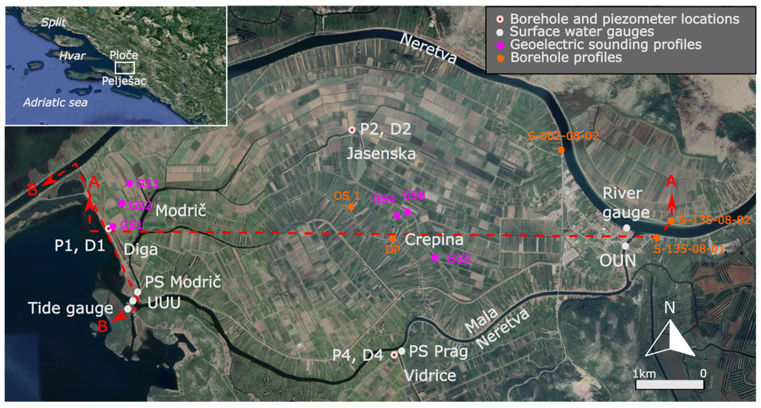
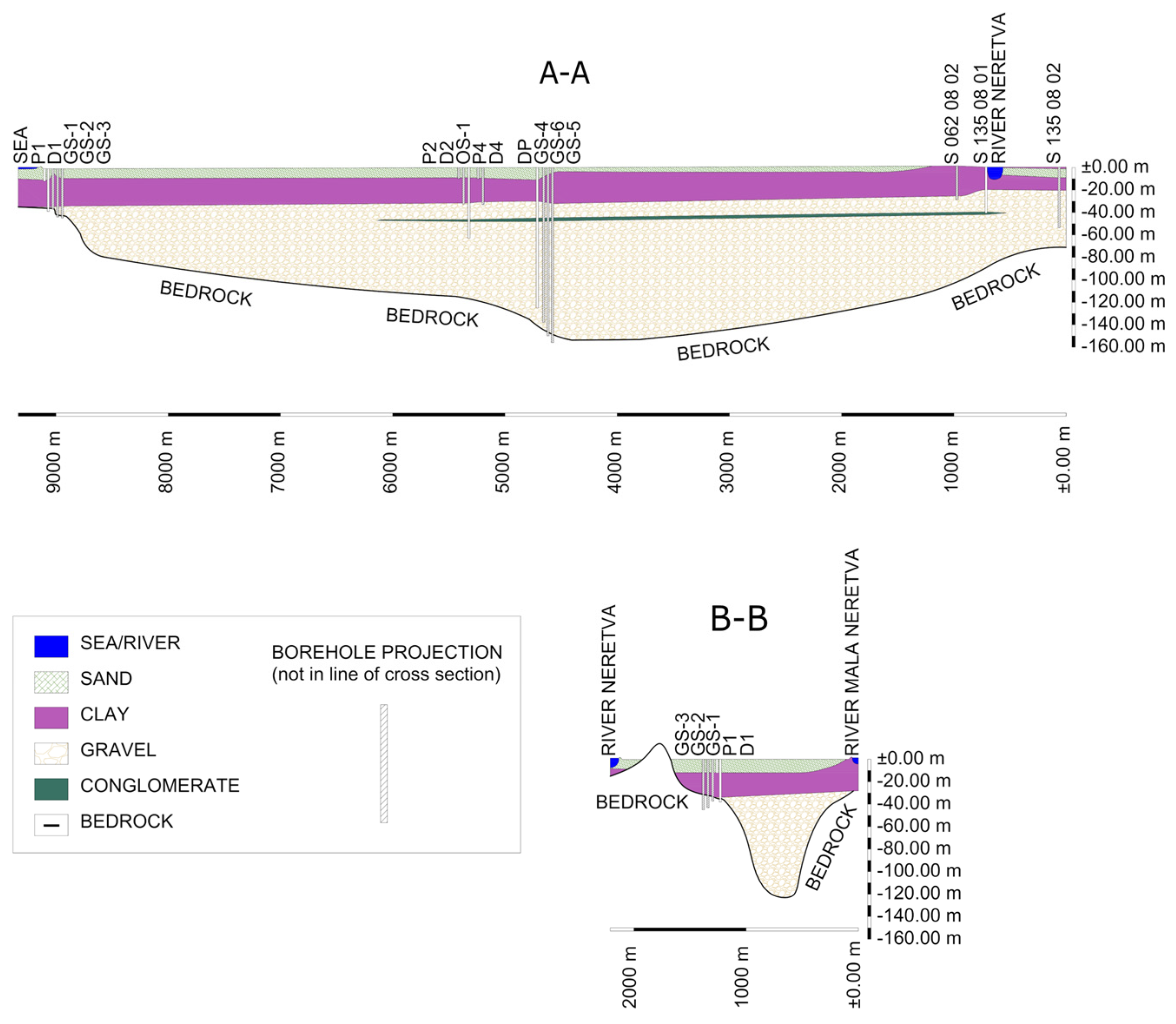
2.1. Neretva Coastal Aquifer

River Neretva Valley is located in the southern part of the Republic of Croatia and represents the biggest cultivated area in coastal area of the country. It is surrounded by the Adriatic Sea to the west and karstic hills to the north, east, and south (Figure 1). In the very southern part of Vidrice area, several small karstic springs are present and positioned at an elevation of approximately mean sea level. Those springs are activated after certain amount of precipitation, giving brackish to saline water in the early time of activation [32]. Due to the fact, their location is 100 m away from the main channels feeding the PS Prag with water, most of this saline to brackish water ends up in the channel.
River Neretva represents a typical fluvial stream passing through the valley and ending up with mouth in the Adriatic Sea. The Neretva Valley covered about 4500 hectares of primarily marsh area until mid of 20th century. In 1960s and 1970s, infrastructure work ended up in land reclamation of Modrič area by construction and implementation of the embankment Diga creating the present coastline, melioration infrastructure and pumping stations designed to drain the water from the valley to the sea, thus reducing the groundwater level and creating preconditions to start with modern/profitable agricultural production. The conceptual solution of the melioration system relies on a large number of channels converging towards two pumping stations, Modrič and Prag, respectively. Pumping station Modrič is located in the very southwestern part of the valley, approximatively 30 m away from the sea. Melioration channels from Jasenska, Crepina, and Diga areas converge on the Modrič pumping station intake with water. With an installed capacity of 19 m3 s−1 [32], water is pumped to the sea thus keeping groundwater below the pedological layer. Apart from this, the whole southern territory of the valley, called Vidrice, is meliorated by a similar system, ending up with pumping station Prag with installed capacity of 7 m3 s−1 [32], that pumps the water to Mala Neretva that finally carries it downstream to the sea. Mala Neretva is today a closed system, with gates installed upstream in the town of Opuzen and downstream at the mouth. Originally, Mala Neretva was designed for flood protection but up to date its dominant function is to provide the only source of freshwater during dry periods when the water is supplied by the upstream area, close to the border with Bosnia and Herzegovina. Neretva valley area has pretty flat terrain, with elevation ranging from −1.90 to +2.40 m a.s.l. with “Nula Trsta” used as a referent vertical datum.
River Neretva is characterized by typical inter-seasonal discharge fluctuations with an average precipitation of 1200.78 mm year−1 observed at Ploče meteorological station and 1219.91 mm year−1 observed at Opuzen meteorological station for the period 2009–2018. Discharge varies between 40 m3 s−1 up to 2600 m3 s−1. The highest value corresponds to 1000-years return period [33] and was observed after the occurrence of long-duration rainfall at the river Neretva catchment area located mostly in the territory of neighboring Bosnia and Herzegovina. The usual range of discharge found at the study area ranges from 40 m3 s−1 up to 1800 m3 s−1. The abovementioned lower limit is caused by controlled release of the biological minimum 47 km upwards from the Opuzen, at the hydro power plant of Mostar. Mean long-term average annual discharge corresponds to 290–330 m3 s−1. Significant differences in discharge values are present during the hydrological year. Summer season is identified as the dry one, with on average no more than 100 mm month−1 of the precipitation, mainly concentrated within few days, thus representing isolated rainfalls. The discharge dominating the period from mid-May until late September slightly ranges from 40 to 200 m3 s−1. Isolated discharge peaks are mainly found in period from November to April, as a consequence of intensive precipitation within the catchment area. Those peaks frequently exceed 1600–1800 m3 s−1.
Based on available hourly data sets observed by Croatian Hydrometeorological Institute meteorological station Ploče, the minimum observed temperature for the period 2008–2019 equals to −7.80 °C, whereas the maximum is 38.80 °C.
Tidal induced sea level fluctuations in the area of interest are of mixed diurnal–semidiurnal character. In a study by Srzić et al. [18], four dominant tidal constituents were identified in sea level observation, contributing to more than 95% of observed sea level fluctuations, namely O1 and K1 as diurnal constituents and M2 and S2 as semi-diurnal constituents. O1 has been determined with amplitude of 0.0201 m and a phase of 159.80°, K1 with an amplitude of 0.075 m and a phase of −93.45°, M2 with an amplitude of 0.0942 m and a phase of −29.55°, and S2 with an amplitude of 0.0729 m and a phase of −3.33°. These constituent characteristic values correspond to one-month duration signal observed during August 2015. Typical on average tidal amplitude corresponds to approximately 18 cm.
Starting form 1960s up to date, a comprehensive in situ geotechnical and geophysical investigation work has been performed [32,34,35,36,37,38,39,40,41,42]. By summing up all materials from the conducted in situ work and their interpretation, the general geological structure of the area has been reconstructed as shown in Figure 2. The top layer corresponds to a dominantly fine sand with less than 1.0 m thick sub-layers of clay and mud present locally in the central and near shore area. Towards north east and along the left bed of river Neretva, clay has been found even close to the ground surface. Sandy layer mimics the upper unconfined aquifer with overall thickness of 1–10 m. Beneath the unconfined sandy layer, a compact clay layer has been determined along the whole study area, thus creating a low permeable confining geological layer. The thickness of this layer varies between 10 and 25 m and slightly increases towards the sea. A compact clay layer continues beneath the seabed offshore. Stratigraphically below the confining clay layer, a mostly coarse gravel layer, with the partial presence of mud and fine sand thin sublayers, has been identified with overall depth of 10–15 m. Borehole cores taken from this geological unit found a high permeable gravel material with an average grain diameter of 42 mm [2]. In the central, northern, and southern area of interest at depths ranging from 40 to 45 m, a conglomerate layer whose thickness ranges from 1 to 3 m locally is present/found. It is important to emphasize that this is a local feature that was not detected at all available boreholes, thus suggesting its discontinuity. The extension of gravel layer is found beneath the conglomerate unit, mostly made of medium and fine gravel with overall depth being defined by the absolute elevation of the bedrock. The bedrock of the area was found as limestone by geoelectrical sounding [35] and by boreholes [34,41] at the absolute depth of zero at the edging valley area, to a maximum of 165 m below ground level found at the very central part of the valley, called Crepina.

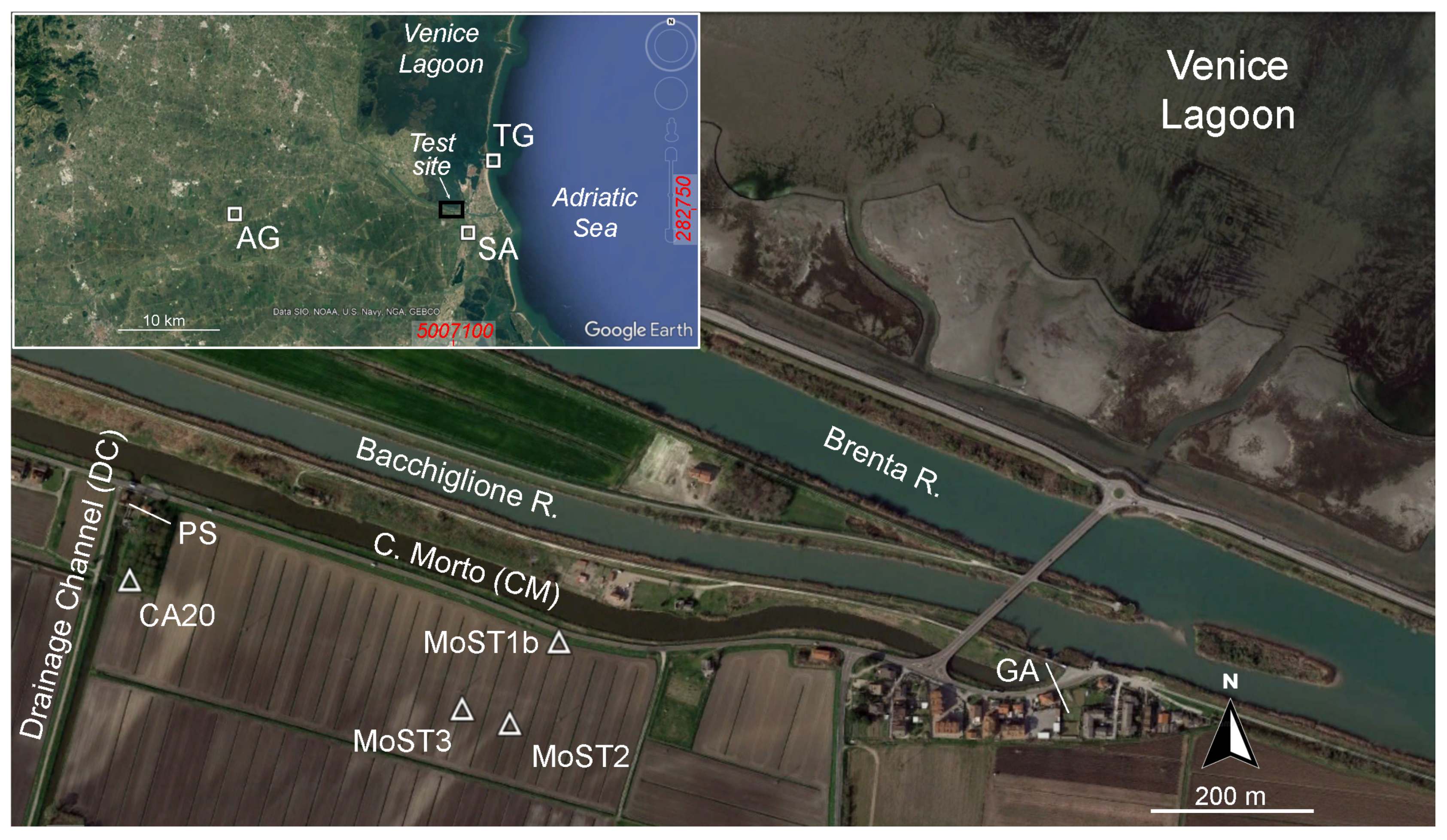
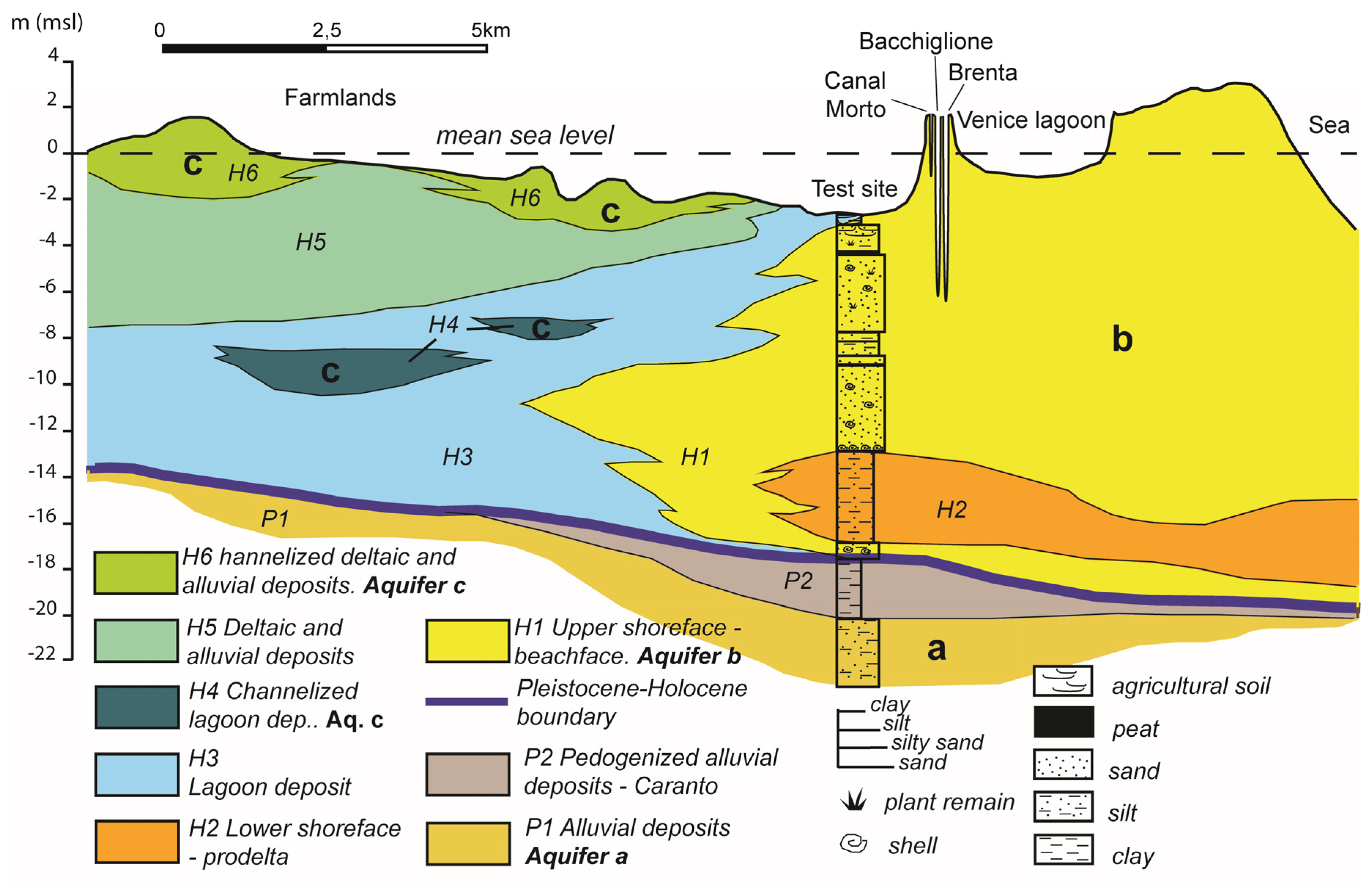
2.2. Venice Coastal Aquifer

The Venice study site is adjacent to the southern lagoon margin and located in a farmland area just south of the Brenta and Bacchiglione rivers (Figure 3).
The Venice region is part of the Po River plain, a foreland region located between the NE-verging northern Apenninic and the SSE-verging eastern South-Alpine chains [43,44]. Focusing on the geological setting of interest for this study, the sedimentary sequence consists of Late Pleistocene and Holocene deposits represented by different alluvial facies and transgressive marine—back barrier sedimentary units, respectively (Figure 4). In detail, the Late Pleistocene deposits, which are included in the first 20–25 m of subsoil (maximum depth of interest for this study), consist of alluvial sand, silt, and clay. The top is dated about 18,000 years BP and shows evident signs of pedogenesis, i.e., the caranto layer (an overconsolidated clay quite common in the area, e.g., [43,45,46] and a regional unconformity) [47]. The beginning of the Holocene sedimentation ranges from 9000 to 8000 years BP [48,49]. The sequence shows the typical wedge-shaped architecture containing transgressive and highstand deposits (Figure 4). The transgressive sequence frequently shows a thin basal layer of lagoon/back-barrier deposits that gradually changes in over-flood facies towards the mainland. The transgressive deposit continues upwards, establishing heteropic relationships among lagoon, littoral, and shelf deposits depending on their position with respect to the past coastlines. The successive units are related to the progradational system due to the sea level highstand: generally, they show heteropic facies from fluvio-deltaic to lagoonal and gradually passing to littoral and shelf (Tosi et al. [47]). In the study area (MoST site in Figure 3), the transgressive deposits are composed by a thin basal layer of littoral sand passing upward to laminated silt, silty clay and silty sand interpreted as pro-deltaic deposits. The highstand succession shows 10 m thick littoral sandy deposits, locally topped by a thin layer of lagoon silt.
The heteropic relationships among littoral, deltaic, lagoon, and alluvial deposits led to the development of a complex hydrogeologic system, including, confined, locally confined, and unconfined aquifers. Considering the upper 25 m of the subsoil, it is possible to recognize three main aquifer types: (i) a semi-confined aquifer (Figure 4a), located in the Pleistocene alluvial deposits at around 20 m depth and locally confined at the top by the caranto layer, (ii) an unconfined aquifer, located along the coastline in the sandy littoral deposits (Figure 4b), (iii) local smaller aquifers, from confined to semi-confined in sedimentary bodies as paleo-channels or remnants of littoral ridges located towards the mainland (Figure 4c). Furthermore, over historical time, the hydraulic setting of this territory shifted from natural to completely artificial. Starting from the 15th century, the Most Serene Republic of Venice diverted the Brenta river mouths out of the lagoon, close to the study area, in order to prevent the generalized filling of the lagoon basin. Then, at the beginning of the last century, extensive hydraulic reclamation works carried out in most of the Venice coastlands transformed part of the lagoon margins and wetlands into farmlands. Today most of the territory that includes the study site, lies below the mean sea level and is mechanically drained by pumping stations to make agricultural activity profitable and to avoid flooding during adverse meteorological and meteo-marine conditions. A complex network of drainage ditches and canals vehiculate the runoff from the land to pumping stations in order to regulate the hydraulics and discharge the excess water into the Venice Lagoon or the Adriatic Sea.
Due to the proximity to the sea and the lagoon, shallow costal aquifers and farmlands are affected by saltwater intrusion. Past studies, e.g., [28,30,31], revealed that groundwater salinization is driven by the superposition of various factors, such as the general low-lying of the coastal plain, the complexity of the hydro-stratigraphic setting, tide encroachment along river mouths and the mechanical drainage. Preferential groundwater flow pathways from the lagoon basin to the mainland establish through sand structures of paleochannels and the seawater encroachment into the river mouths extends up to some tens of km inland the saltwater contamination.
Specifically, the groundwater dynamics in the study area (both levels and salinity) is controlled by the local precipitation, the sea-lagoon water level (that is controlled by the tide), the mechanical drainage regulated by the Casetta pumping station, and the Brenta-Bacchiglione river system together with the Canal Morto (Figure 3).

3. Methodology

3.1. Monitoring Systems

The monitoring systems in the study areas have been planned, implemented, and put into operation and represent pilot implementation of a comprehensive interregional project. A sequence of the monitoring system installed at Croatian site comprises an existing monitoring system with improvements done with the interregional project. The monitoring methodological approach is shown separately for two systems in the following. For sake of completeness and clearness, a unique variable identification procedure within the text has been used from this section on: (i) “T” is used to denote temperature [°C] variable, (ii) “EC” as electrical conductivity [mS cm−1]; (iii) “P” as pressure [mbar]; and (iv) “h” as piezometric head [m a.s.l.] and/or surface water elevation.

3.1.1. Neretva Valley Aquifer System

A monitoring system has been installed and set up recently at Neretva Valley to observe h and seawater intrusion parameters as shown in Figure 1. A tide gauge station has been installed close to the Mala Neretva mouth while Neretva surface elevation gauge has been located at the left side of Neretva river bed in Opuzen town. Two additional surface water elevation gauges are installed at Mala Neretva river, one downstream from the gate in Opuzen, identified as OUN, and the other one, UUU, upstream from the gate at Mala Neretva mouth. Both types of stations are equipped with the instrument/shaft encoder THALIMEDES OTT with a sampling frequency of 1/hour, measuring range of ±19,999 m, resolution of 0.001 m, and accuracy of ±0.002 m.
EC, h, and T in unconfined aquifer have been observed at three locations identified by P1, P2, and P4 on Figure 1. For h observations, OTT ORPHEUS MINI vented gauge has been used and set up to sampling frequency of 1/hour with measuring range from 0 to 40 m and resolution of 0.001 m. A MANTA 2 40+ gauge has been installed to observe groundwater EC and T in piezometers. This gauge has a measuring range of 0 to 100 mS cm−1 with an accuracy of ±1% and 0.0001 mS cm−1 resolution for the EC standardized to 25 °C. The T sensors range is −5 to 50 °C with a resolution of 0.01 °C and an accuracy of ±0.1 °C. Piezometers have been drilled and penetrated in unconfined aquifer with a finite depth of 10 m below the ground level with inner diameter of 12 cm. The height of perforated screen equals to 9.50 m starting from piezometers at bottom. Gauges have been installed 2.0 m above the piezometer bottom.
Within the piezometers, penetrated to deep confined aquifer, TE Connectivity TRUBLUE vented gauges with a 0 to 300 psi range and accuracy of +/−0.05%, Total Error Band (TEB) have been installed to observe h values at three locations, respectively, D1, D2, and D4. For the D1 piezometer, overall piezometer depth was set up to 38.30 m, with a perforation height of 1.20 m within the confined aquifer, beneath the confining clay layer. Piezometer D2 overall depth equals to 30.80 m, with a perforation height of 3.0 m within the gravel media to ensure the insight to confined aquifer piezometric state. For the piezometer D4, the overall installation depth was set to 32.87 m, with a perforated depth of 2.0 m within the confined aquifer. The inner diameter of confined aquifer penetrating piezometers corresponds to 8.0 cm. The installation depth of gauges corresponds to 10 m below piezometers top.
For all the piezometers employed in the study, the filter layer was built of the material of higher conductivity than natural material at the location in order to avoid signal attenuation. Observations from installed gauges were temporally synchronized relative to the unique temporal origin set up within the data acquisition system. Observation of all parameters covered by this study has been done every hour while h values are expressed relative to “Nula Trsta” vertical datum.
For the purpose of this study, two periods were selected as relevant for Neretva coastal system, rain and dry period, respectively. Relying on the amount of precipitation, February 2019 was selected to represent the rain period, while July 2019 was selected to represent the dry period. All data sets have been shown with frequency 1/hour except the precipitation, which corresponds to cumulative daily value.

3.1.2. Venice Aquifer System

The aquifer system of the study site has been monitored through three piezometers screened approximatively from the top to the bottom in the phreatic aquifer (piezometersMoST1b, MoST2, MoST3) and one piezometer screened between 15 to 20 m (CA20) in the locally confined aquifer (Table 1).
P, EC, and T data have been recorded by CTD Divers® logging sensor in piezometers MoST1b, MoST2, and MoST3, while only P in piezometer CA20 (Table 1). MoST1b, MoST2, MoST3 piezometers have been setup with two sensors, approximatively at the top and the bottom of the phreatic aquifer (Table 1).
P, EC, and T have been recorded with a 10-min frequency from 16 July to 22 October 2020 in MoST1b, MoST2, MoST3 and from 1 July to 31 October 2020 in CA20 piezometer.
In addition, EC and T vertical profiles have been acquired at least 2–3 times/month in all piezometers. Piezometric head (m a.s.l.) has been obtained through barometric compensation of P data using atmospheric pressure recorded by BARO-Diver® and referred to the Italian geodetic datum.
Regarding the hydrologic conditions of the study area, the water levels of the drainage have been measured in the intake channel of the pumping station and in the Canal Morto at the outflow of the pumping station (DC and CM in Figure 3. Sea level data were obtained from the Chioggia tide gauge station (data available from: https://www.comune.venezia.it/it/content/6-diga-sud-chioggia (accessed on 21 February 2021)) and daily rainfall data by the weather station of Sant’Anna (data available from: https://www.arpa.veneto.it/bollettini/storico/Mappa_2020_TEMP.htm (accessed on 21 February 2021)) (TG and SA in Figure 3).

3.2. Time Series Analysis

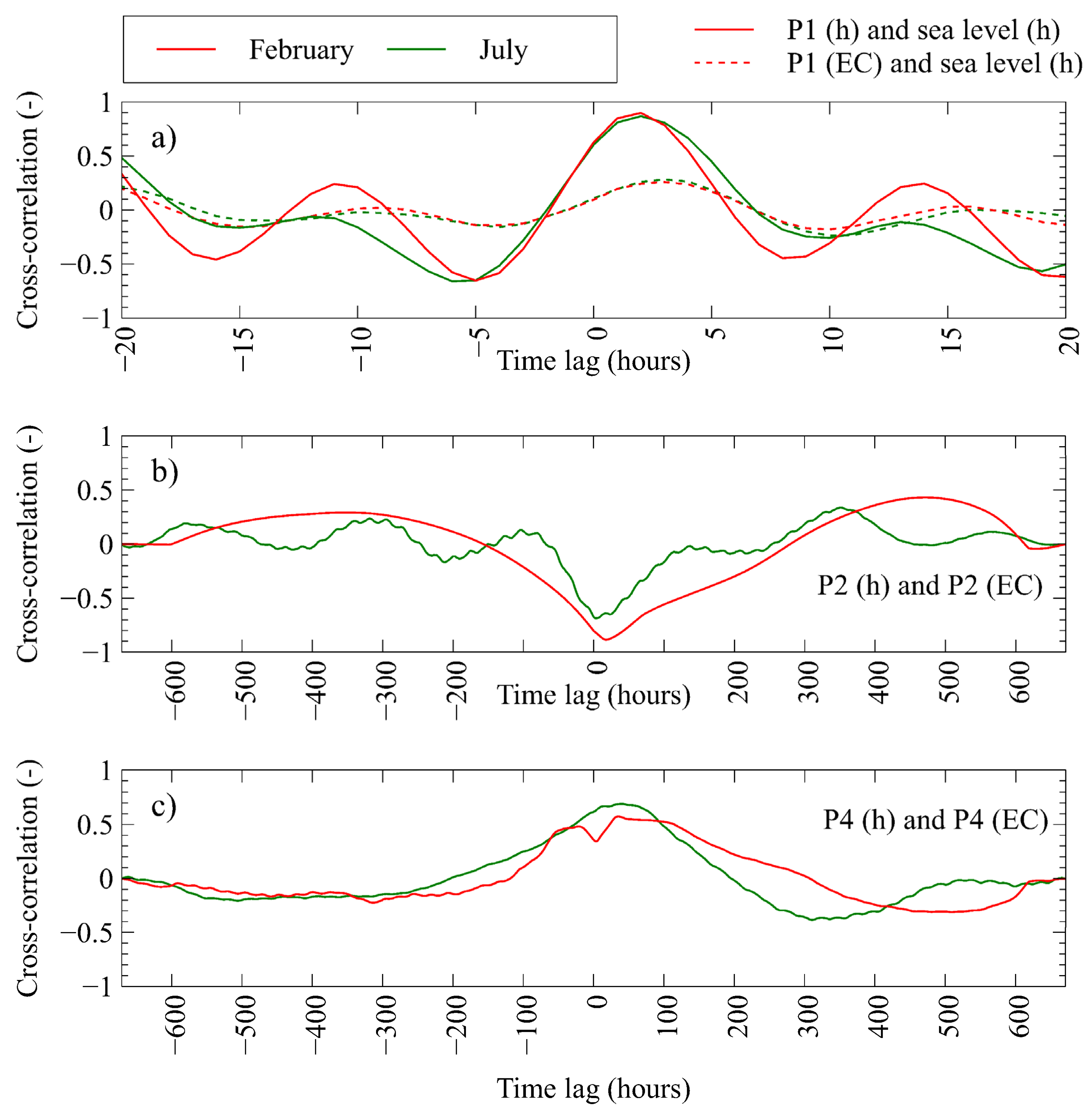
3.2.1. Cross-Correlation Analysis

A cross-correlation model was applied to time series to identify and quantify the relationship between different aquifer input signals such as sea level and aquifer output signals in boreholes, respectively, piezometric head and EC. Auto-correlation is used to describe the periodicity of a signal. If a signal has a strong periodicity, then auto-correlation function will have a small decrease with time shift and if a signal has non-periodic behavior then auto-correlation function will have a sharp decrease. Auto-correlation function is calculated by, Equation (1):
a ( τ ) = C o v X X σ X X σ X X = E [ ( X t μ X ) ( X t τ μ X ) ] E [ ( X t μ X ) 2 ] E [ ( X t μ X ) 2 ]   ( )
where a(τ) is the auto-correlation function, τ is the time shift, CovXX is the cross-covariance, σXX and σYY are standard deviations, E is the expected value, µX is the mean value, and X is the variable of interest. The cross-correlation quantifies the similarity between two signals as a function of time lag in between [50]. The cross-correlation function is calculated by, Equation (2):
c ( τ ) = C o v X Y σ X X σ Y Y = E [ ( X t μ X ) ( Y t τ μ Y ) ] E [ ( X t μ X ) 2 ] E [ ( Y t μ Y ) 2 ]   ( )
where c ( τ ) is the cross-correlation function, τ is the time shift, CovXY is the cross-covariance, σXX and σYY are standard deviations, E is the expected value, µX and µY are mean values of X and Y variables of interest.

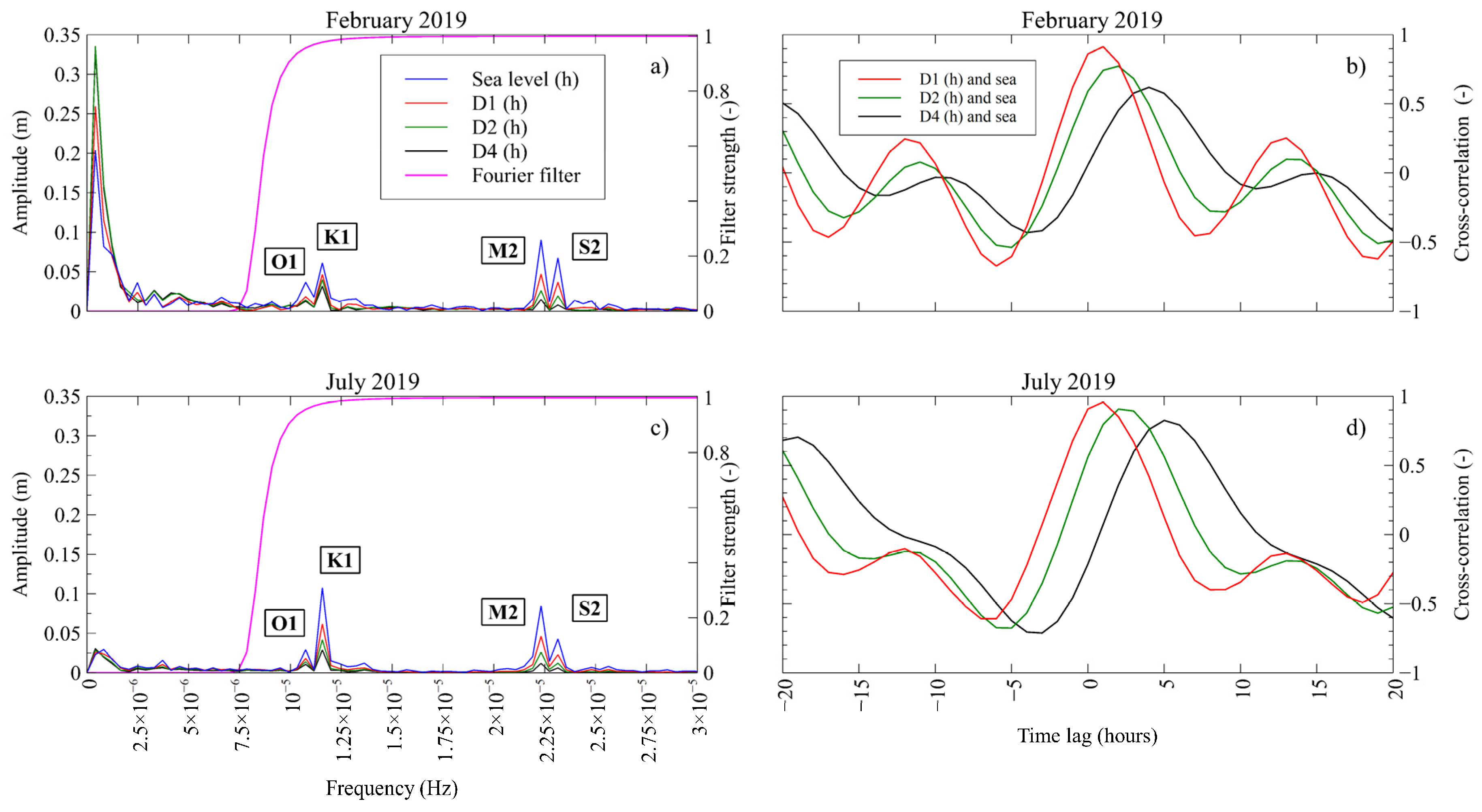
3.2.2. Spectral Domain Analysis

Transformation of observed time series from temporal to spectral domain has been done by Fast Fourier Transform (FFT) application incorporated in Python SciPy library either in R (packages ‘xts’, “TideHarmonics” and “TSA”), thus enabling the insight to time series periodicity and structure of observed signals in way of constituent contribution to observed signal definition. FFT results are of a complex type where absolute value of complex number is recognized as magnitude of given frequency and angle between real and imaginary component in FFT result is recognized as phase of given frequency [51]. Amplitude of each frequency can be obtained by normalizing magnitude results with number of samples [52]. Amplitude spectral density (ASD) is often used for visual interpretation of FFT results [18,53,54] from which amplitude and period values of each constituent in frequency bin can be easily read, while phase was calculated from FFT results [51].
Signal detrending has been done by Fourier magnitude filter [51]. Filtered signals are absent of all external stresses except tidal stresses and signal noise which is considered negligible. Detrendend signals are used for the identification and quantification of tidal influence on coastal aquifers [55,56]. Filtered signals were reconstructed from frequency domain back to time domain with Inverse Fast Fourier Transform (IFFT) also incorporated in Python SciPy library, thus enabling further analysis of detrended signals in time domain. A similar detrending method is used in the Reference [57].

4. Results

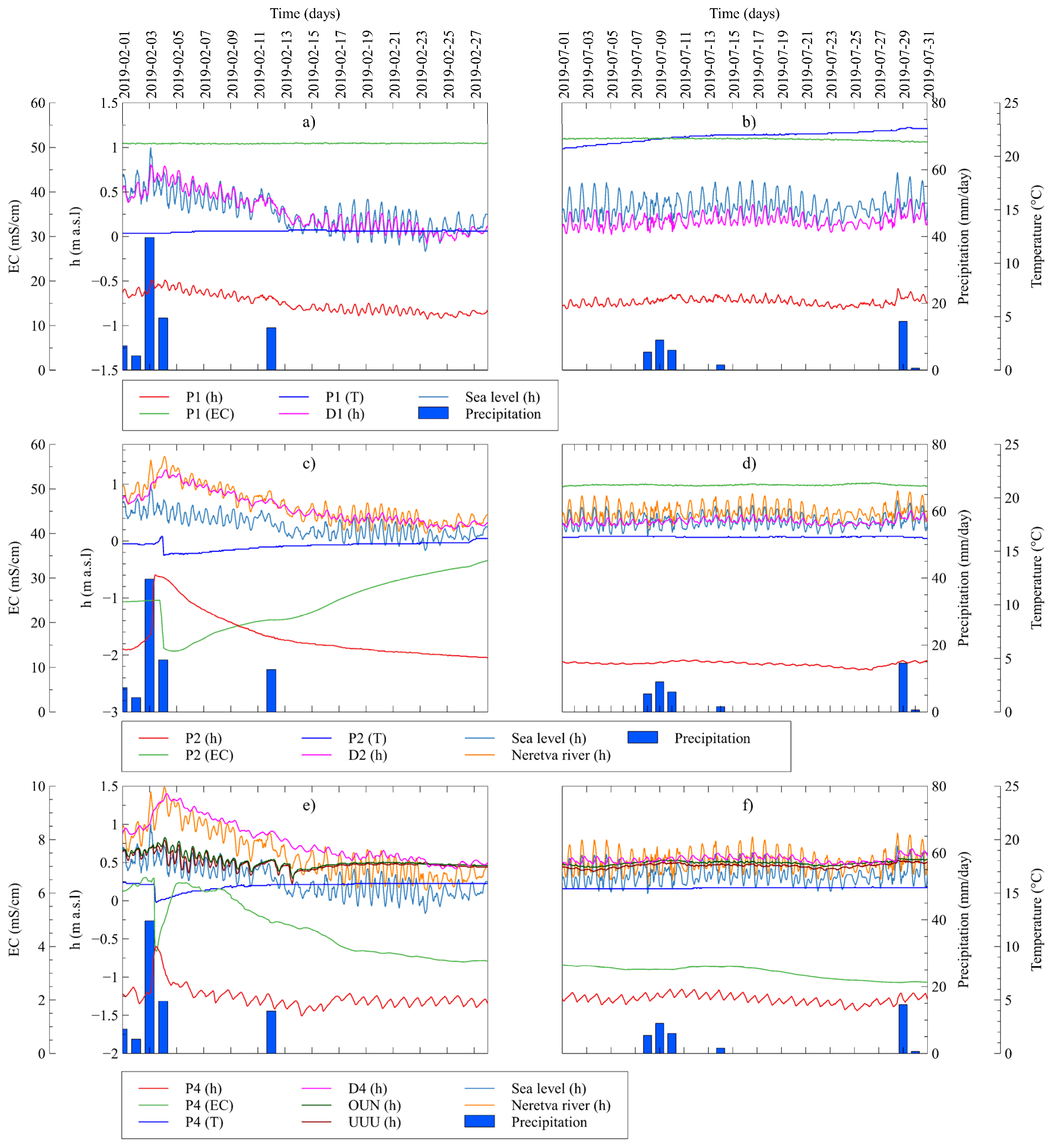
4.1. Neretva Valley Aquifer System

A comprehensive overview of observations taken from Neretva coastal aquifer system is shown in Figure 5a–f, representing both rain and dry periods as well as three monitoring locations covered by the study. Following observed times series in Figure 5, a periodic nature of confined aquifer h time series, similar to those of sea level ones, can be observed. This feature has been previously identified and analyzed to obtain hydrogeological parameters [50,58,59]. During the July 2019 (Figure 5b), D1 piezometric head is constantly kept below sea level, with an average tidal efficiency [58] (TE) equals to 0.63. During the first half of February 2019, the occurrence of a four-day period (February 1st–4th) of precipitation with maximum amount of 39.7 mm day−1 increases the D1 h average value with D1 h values being even greater than sea level ones (Figure 5a). This is explained as a consequence of increased groundwater recharge from inland caused by precipitation, which diminishes with time since precipitation occurrence. Similar findings were present in work by Kim et al. [60].
Compared to D1, piezometer D2 located approximately 4.50 km inland from the Diga coastline is characterized by on average higher h values compared to D1 but with increased attenuation of signal amplitude corresponding to TE value of 0.45 (Figure 5d). The increase in D4 h due to the groundwater recharge component caused by precipitation and related subsurface inflow from catchment area during the first half of February 2019 equals to 48 cm, which makes this location most sensitive to groundwater inflow component (Figure 5e,f). By coupling observed piezometric features in D1, D2, and D4, it is obvious that the groundwater flow within the confined aquifer is directed from east and southeast towards the shoreline located to the west. This is in agreement with previously performed studies [32]. The latter holds for both dry and rain period.
The amplitude spectral density (ASD) of D1, D2, and D4 h signals in Figure 6a,c implies the sea level as a main driving force resulting in groundwater h oscillations as found within the confined aquifer. As evidenced in Figure 6, the sea level trend is characterized by four dominant tidal constituents, M2 and S2 as semidiurnal, and O1 and K1 as diurnal ones. Constituent characteristic values of sea level and h time series are shown in Table 2. Amplitudes and periods are derived from the ASD in Figure 6a,c, while phase values are calculated for each tidal constituent from FFT results as explained in Methodology section. Both rain and dry periods show dominance of tidal constituents in groundwater piezometric head, thus emphasizing the effect of direct connection of this geological unit with the sea. There is an evident dominance of low-frequency components present during rain period (Figure 6a), which is an effect caused by both trends and meteorological changes, especially precipitation followed by the decrease of barometric pressure. The latter is of minor impact in groundwater piezometric head time series recorded during dry period (July 2019).
While the decrease of the TE is visible through ASD components as the distance onshore increases, time lag values are obtained based on cross-correlation analysis. Prior to analysis, signals are detrended by application of Fourier magnitude filter, which enables the removal of components characterized by periods higher than 44 h. The latter ensures the removal of non-tidal cause periodicity like barometric pressure changes, air temperature change caused features, etc. Cross-correlation functions are shown in Figure 6b,d for both analyzed periods. Results demonstrate a significant correlation between sea level and h time series in confined aquifer with values decreasing with distance increase from shoreline. Maximum obtained cross-correlation value equals to 0.93 and corresponds to sea level and D1 h observed during July for time lag of 1 h. During the rain period, the maximum value of cross-correlation function is reduced to 0.90 with the same time lag value. Compared to D1, piezometers D2 and D4 are shown to be more influenced by components different than diurnal and semidiurnal tidal ones during dry and rain period. During July 2019, maximum D2 h cross-correlation function value is found to be 0.88 for 2-h time lag relative to the observed sea level time series. During rain period, cross-correlation function value is reduced to 0.81, still demonstrating significant influence of the sea level to groundwater h. The highest difference in cross-correlation values between dry and rain periods are found for D4 piezometer. While cross-correlation function corresponds to 0.802 in July, it is decreased to 0.70 in February as well as the time lag change, which has been decreased from 5 to 4 h.
Unconfined aquifer observations offer an insight to groundwater level h, EC, and T as shown in Figure 5. Independently of the piezometer location and the period when observation has been done, groundwater level h is lower compared to one characterizing confined aquifer. This is caused by the artificial water drainage/management operated by the pumping stations whose intention is to keep groundwater low ensuring better conditions for agricultural production all over the study area. Apart from confined aquifer, h value in unconfined aquifer is significantly influenced by external loadings, such as precipitation, and shows dominant effect of PS regimes at the same time.
Although P1 piezometer is located only 40 m from the melioration channel, the dominance of the sea water and its influence on groundwater parameters is evidenced in Figure 5a,b. Independently of the season, no significant changes in groundwater h even during intensive precipitation have been detected, keeping the presence of neap and spring tides within the P1 h time series. EC value changes slightly over the periods of interest.
During February 2019, EC took almost constant value of 50.89 mS cm−1 while a slight increase is observed in June (51.88 mS cm−1). Since the groundwater h value is lower than the sea level, there is an active sea water intrusion process [Bakker 2015.], resulting in P1 EC values close to EC values of the seawater. Following Figure 7a,h shows significant cross-correlation with sea level: 0.90 in February and 0.84 in June, with time lags of 2 h. Apart from h, EC shows dependency on sea level as well, with maximum cross-correlation function value of 0.25 and 3-h time lag (February) and 0.30 and 4-h lag (July). Differences in cross-correlation values and appropriate time lags between the sea level and P1 EC values imply the balance effect between dominance of drainage channel level and of sea level. During the dry season, the pumping system works with minimum capacity due to the scarce precipitation, therefore the sea level assumes a dominant role in determining P1 groundwater characteristics. During February 2019, the system operated on a higher capacity with a total of 784 operating hours combined on all pumps, thus causing a deflection from the state found during dry season where less than 300 operating hours were recorded. Since the distance from the channel to P1 piezometer (40 m) is smaller compared to P1 and coastline distance (80 m), reduced cross-correlation value of sea level and P1 EC (0.25) as well as reduced time lag (3 h) implies the dominance of the drainage channel influence to parameters observed within P1 piezometer. T time series from P1 additionally emphasize the interconnection with sea water. In February, mean T was 12.98 °C while in July it reached 21.82 °C with a tendency of a constant increase due to the increased insolation time.
Compared to P1, time series in P2 show sensitivity to precipitation occurrence (Figure 5c,d) through the h, EC, and T values. After 39.7 mm day−1 precipitation rate, h was increased for 1.31 m and was followed up by a decrease in both EC and T. EC value decreased for 11.4 mS cm−1 while groundwater temperature gauge detected a decrease of 1.8 °C. The dry period offers more stability in observed time series without significant changes. This is explained by the inspection of precipitation occurred during dry period. Precipitation absence leads to the convergence of GW parameters to stable behavior without trends. It is important to notice the EC value in July (50.9 mS cm−1 on average) is higher than that obtained for February (24.55 mS cm−1 on average), same year, showing the importance of precipitation occurrence. Precipitation enhances the dilution of the saline and brackish water by ensuring the volume of fresh water at the surface water bodies found within channels. This leads to long-term reduced GW salinity observed during rain period. Cross-correlation function defined for P2 piezometric head and EC in February results in maximum value of −0.88 fitting to time lag of 18 h (Figure 7b). On the contrary, the dry period results in −0.68 cross-correlation value and only 2-h time lag. The difference in time lags implies the effects of spatially global changes during rain period and their influence on P2 EC state, while during dry period, groundwater features within P2 piezometer are dominantly defined by local conditions in the nearest area.
Piezometer P4 is located 20 m from PS Prag intake and 40 m from the Mala Neretva riverbed. As observed at P4, h shows a significant influence of PS Prag, which is mostly operated in night regime (Figure 5e,f) which explains the daily corresponding frequency in P4 h observations. Due to the small distance from PS Prag intake, even the higher amount of precipitation does not lead to a significant h increase (Figure 5e). Strictly, the increase in P4 h during the period February 3rd–February 4th is lower compared to P2 increase caused by same precipitation (h change equals to 0.75 m while P2 h change is 1.31 m). The same figure demonstrates that the maneuver of opening the UUU gates does not influence P4 h, although the regime of Mala Neretva river has been changed drastically as recognized via presence of tidal constituents within OUN and UUU time series. This implies that the Mala Neretva riverbed has low permeability which is ensured by the construction features of its embankment. Groundwater temperature emphasizes constant value over analyzed periods except for the local decrease of 1.9 °C after precipitation observed on 3 February. EC value shows an initial increase but after the precipitation reaches a value of 39.7 mm day−1 it underwent a decrease of 2.74 mS cm−1. On February 4th, after the precipitation of 39.7 mm day−1 on the previous day, EC value shows an almost linear increase with a tendency to converge to some value of 6 mS cm−1. The remaining period shows that the increase in h leads to EC increase and vice versa. Cross-correlation functions calculated for P4 h and EC values show maximum values of 0.57 and 35-h delay in February and 0.69 and 37-h delay in June (Figure 7c).

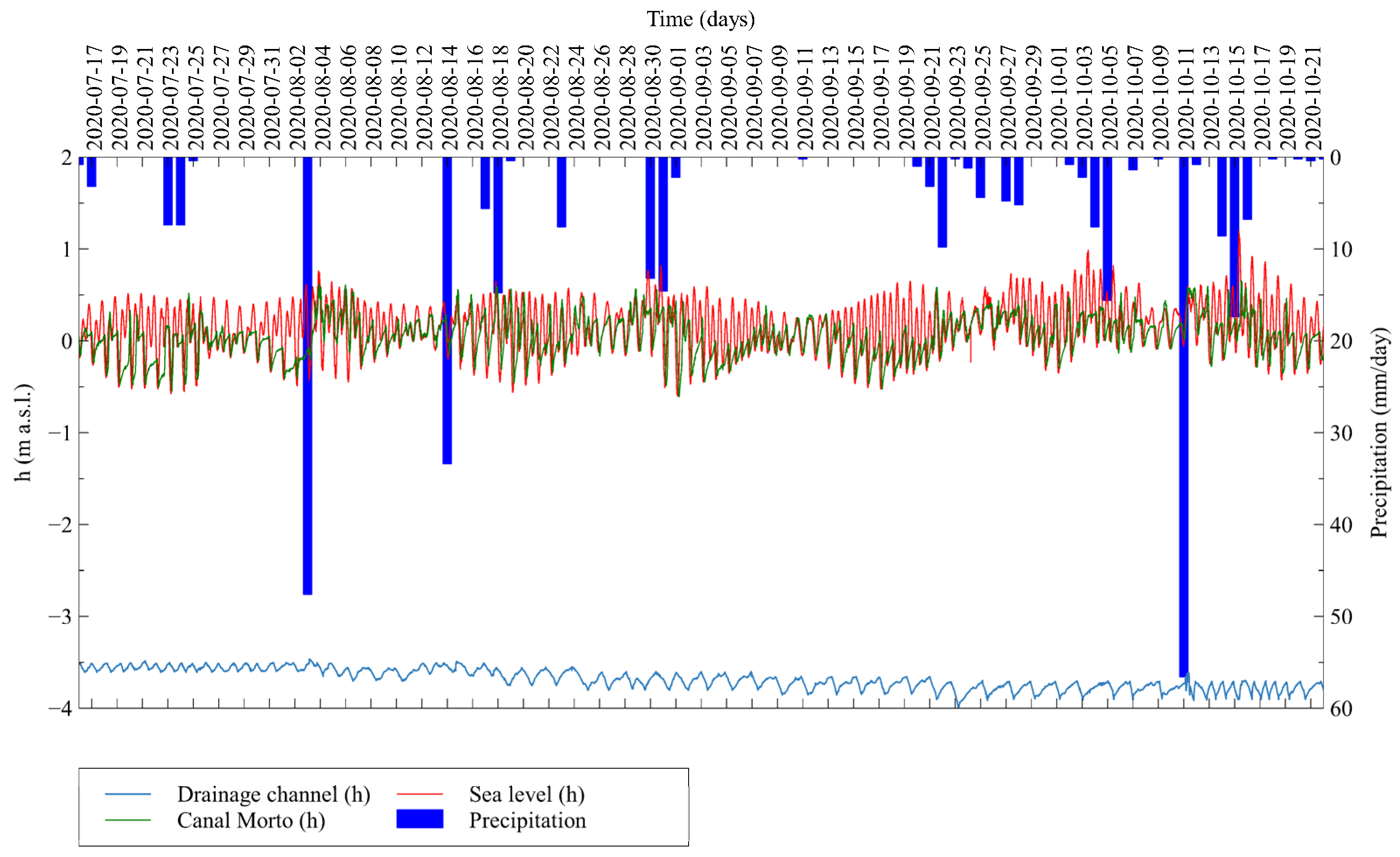
4.2. Venice Coastal System

In this section, the main factors—such as precipitation sea level, Canal Morto, and drainage channel levels—potentially controlling the groundwater dynamics and the data recorded in the shallow locally confined and phreatic aquifers are analyzed.

4.2.1. Forcings

The precipitation regime is characterized by sporadic and quite intense short-term precipitations in July and August, which increases in both frequency and amount in mid-September-October, with some peaks typical of the extreme conditions for this region (Figure 8). TG time series shows the semidiurnal cycle, characteristics of the Adriatic Sea [61] with an approximate maximum amplitude of 1 m and a slightly increasing trend towards the fall season. The CM h value follows that of the sea but with the higher levels significantly reduced by tide GT located at the confluence of the canal with Bacchiglione-Brenta river system. The flow in the canal is in fact strongly dependent on the passive action of GT which, in turn, depends on the interaction of the water levels in the different part of the hydraulic node, i.e., stage/discharge in the two rivers, tidal excursion, and pumping operations in the reclaimed land. To note that when heavy precipitation and irrigation practices maintain a high h value in the channel, its flow prevails on the tidal ingression and the GT closure can be delayed until the tide level is sufficiently high to drive an upstream current that closes the gates. Slight differences in timing between the changes of water levels of the CM and the sea also depend on the distance between the measuring stations.
The DC is located at a lower ground level with respect to the watercourses that naturally flow into the sea (i.e., the Brenta–Bacchiglione–Canal Morto system). It collects the surface water from the drainage ditches of the area and its maximum and minimum levels are controlled by the Casetta PS (PS in Figure 3) in a range of levels determined by the requirements of irrigation and agricultural practices. Specifically, the drainage level was increased by 10 cm in July in order to keep the water table high to sustain the crop production, while it was decreased by 20 cm at the end of the harvesting, in September. In addition, a temporary reduction of the drainage levels is imposed when heavy precipitation is forecasted, e.g., during the heavy precipitation that occurred in early August. It is important to highlight the behavior of the h of the drainage channel, which shows higher frequency oscillations in July when the amplitude is lower, and vice versa in September and October. To note in mid-October, the recorded temporary increase in the frequency of the water level oscillations in the drainage channel is due to the need to evacuate larger volumes of water from farmlands following the heavy rains. EC measured in CM is generally around 1–1.5 mS cm−1, rarely higher and in any case always lower than 3 mS cm−1.
Spectral analysis of CM h value highlighted a frequency content dominated by semidiurnal (12 h 30 min) and diurnal (23 h 40 min) periods, respectively, while the PS inflow levels exhibited dominant periods of 50–45 h, the presence of only the diurnal period, and the absence of the semidiurnal oscillation. Hence, the CM h values are clearly related to tides while the regulation of the drainage ditch operates as a low-pass filter, cutting the semidiurnal tidal component and introducing a slower varying sawtooth profile on the pumping levels with a period of about 2 days depending on the pump flow rate, the volume of the reservoir, and the phreatic aquifer recharge through the leakages (along the CM edges).

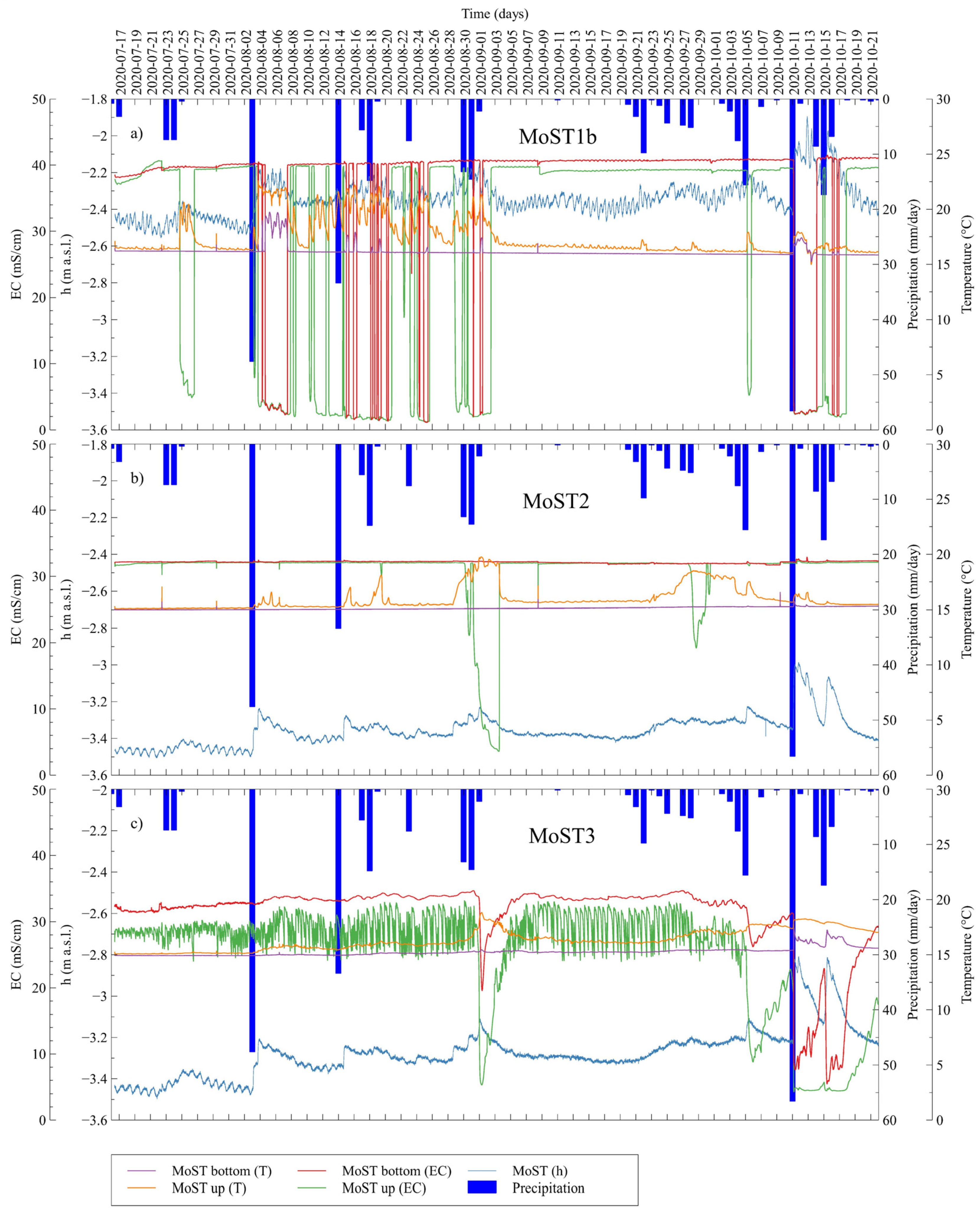
4.2.2. Phreatic Aquifer

The piezometer MoST1b is located in the North-eastern part of the study site, approximately 30 m and 450 m from the CM and the lagoon, respectively (Figure 3). The piezometer is equipped with two sensors, at −3.94 m and −6.48 m a.s.l. h values show an increasing trend of the mean values from −2.5 m a.s.l. in July to–2.3 m a.s.l. in October and very rapid rises of the water table until reaching the highest depth of −1.9 m a.s.l. in mid-October. The water table is also characterized by a daily oscillation with amplitude in the range of about 10 cm (Figure 9a). The EC measured by both sensors shows a background value of about 40 mS cm−1, often interrupted by sudden drops to 2–8 mS cm−1 in correspondence with the water level rises. Groundwater T is in the range of 16–23 °C and 16–19 °C for the upper and lower sensor, respectively, and shows slight increases in correspondence of the EC decreases (Figure 9a). By analyzing together precipitation, h, EC, and T time series, it is clear that the dynamics of groundwater are well correlated with the freshwater recharge during precipitation events and that the freshening effect involves the whole thickness of the aquifer.
The piezometer MoST2, located in the South-eastern part of the study site, is also equipped with two sensors, the upper being placed at −4.11 m a.s.l. and the lower at −7.83 m a.s.l. (Figure 9b). The signature of the h is similar to that of the MoST1b, despite their difference in absolute values that depends on the lower ground elevation of the MoST2 site. It ranges between −3.45 and −3 m a.s.l. in July and October, respectively, and shows high-frequency oscillations with decreasing amplitude from 2–4 cm in July to about 1 cm in September and October. The EC has a background value of about 32 mS cm−1 and shows some sharp decreasing events, of which only two are relevant, up to 4–5 mS cm−1 and around 20 mS cm−1, between the end of August and the beginning of September and at the end of September, respectively. The background value of T in MoST2 is around 15 °C with an increase of up to 20 °C in correspondence with the EC falls and the increase in water level (Figure 9b). Therefore, even the groundwater dynamics at MoST2 are linked to the precipitation, which recharges the aquifer with freshwater. However, the decrease in EC values is reduced compared to MoST1b, and the freshening effect is limited to the upper layer of the aquifer.
The piezometer MoST3 is located in the southern part of the study site and west of MoST2 (Figure 3). It has been equipped with two sensors at −4.03 m a.s.l. and at −10.52 m a.s.l. The piezometric head time series has the same signature as those of MoST1b and MoST2 with a general increasing trend from July (about −3.5 m a.s.l.) to October (about–3.2 m a.s.l.) characterized by high-frequency oscillations decreasing in amplitude from 5 cm in July to 1 cm in October (Figure 9c). The EC shows mean values of about 28 and 34 mS cm−1, in the upper and lower sensor, respectively, and sharply decrease up to 5 mS cm−1 in correspondence of the highest water levels. Higher amplitude oscillations in the range of 2–3 mS cm−1 in July and to 5–8 mS cm−1 in September distinguish this MoST3 site from the other two. T value is about 15 °C, increasing up to 17 °C in phase with the falls in EC and the highest h values (Figure 9c). As highlighted for the other piezometers, most precipitation events induce significant increases in the groundwater level. However, changes in EC and T are here much less sensitive to the aquifer recharge as they are recorded only during major precipitation events.
With the aim of identifying the contribution of the tide and CM and DC water levels on the aquifer dynamics, a cross-correlation analysis between their water levels with the h and EC of the groundwater aquifer detected at MoST1b, MoST2, and MoST3 sites has been performed. Because of the described effect of the daily precipitation in the unconfined aquifer, the dry period 2nd–19th September has been selected to compute cross-correlations.
Observed h and EC at the MoST1b piezometer site are in phase and delayed with respect to the tidal signal (green lines in Figure 10a); the maximum cross-correlation values correspond to +0.55 and +0.12 and the delays are 3 h and 4 h 40 min for the h and EC, respectively. Maximum cross-correlation between h at the MoST1b piezometer and CM levels is in phase without any delay (+0.50 at 0 lags, continuous red line in Figure 10a). Conversely, MoST1b EC correlates with CM levels in phase with about 4h early and maximum cross-correlation 0.16 (dashed red line in Figure 10a). Assuming that the effect of the tide along the CM is minimized by the action of the gates GT at the mouth, the water level changes in the CM should be mainly linked to the upstream water accumulation with slower rise with respect to the that of the sea level with closed GT and the quick downstream discharge, almost simultaneously to that of the sea when the tide recedes and the gates open. Considering that MoST1b level and EC directly rise with CM levels, and that CM brings freshwater, we can assume no direct relationship between them during the rising level, while it occurs during lowering levels. Hence, the freshening of groundwater is not due to the influence of CM but it is likely the effect of leakage from the Brenta–Bacchiglione system, the riverbed is deep enough to intercept the phreatic aquifer. The drainage channel level (pumping station inflow) follows the phreatic aquifer level and, therefore, reaches the maximum water level after the groundwater level has reached its maximum: the maximum cross-correlation between MosST1b water level and the drainage channel is about 8 h 20 min early (0.37, blue continuous line). MoST1b EC and the drainage channel level (PS inflow) show the maximum correlation in opposite phase with 12 h early (−0.2, blue dotted line).
Cross-correlation analysis indicated that sea level is not a driver of h and EC in MoST2 up to 12 h lag. Weak correlations with sea level are observed at 7 h 50 min ahead for h (+0.12) and at 8 h 30 min ahead for EC (−0.09), respectively (green dotted line in Figure 10b). MoST2 h values and EC are correlated in phase (−0.2) and opposite phase (0.20), respectively, 4 h 30 min early with the CM levels. Consequently, we might exclude that CM levels are a driver for the aquifer at MoST2 site. The MoST2 h delays about 3 h 40 min in phase the DC level (0.31, blue continuous line), which is in turn always inversely, though weakly, correlated to the MoST2 EC (minimum cross-correlation −0.2 at 4 h 30 min delay, blue dotted line).
MosST3 h and EC seem to indicate that there is no cause–effect link with tidal forcing (cross-correlation below the limits of significance, Figure 10c, green curve). MosST3 h values lead in counterphase by about 4 h 10 min early the CM level (−0.23, red continuous line), while MoST3 EC directly correlates to CM levels of about 4 h early (+0.24, red dotted line). MoST3 piezometer is in phase with the DC level and exhibits a maximum correlation with 2 h 20 min early (+0.3, blue continuous line). MoST3 EC correlates with the DC (PS inflow) in the opposite phase, with 10 h early (−0.32, blue dotted line).
Summarizing, the cross-correlation analysis combined with the observation of the logged time series recorded in the piezometers confirms the hypothesis that only the drainage channel affects the levels of the phreatic aquifer at both MoST2 and MoST3 sites. The EC background is given by the SWI from the lagoon and the river mouths and is modulated by the freshwater leakage from the Brenta and Bacchiglione river beds especially during the lowering of the tidal level.

4.2.3. Confined Aquifer

CA20 h varies between −1.43 and −1.77 m a.s.l. over the July–November period (Figure 11a), showing daily oscillation frequency, likely linked to the tidal forcing. Maximum values of h frequently occur just after the main raining events. EC measurements, collected during periodic field surveys, are in the range of 31.0–32.5 mS cm−1.
In order to better highlight the influence of the tides on the h values, the spectra contents of the two signals have been computed. The resulting spectra confirms the predominant influence of tides with related harmonics typical of the Northern Adriatic Sea, i.e., semidiurnal tide (M2) and the diurnal tide (K1). In detail, the ASD of sea level computed for the Chioggia site is characterized by amplitudes of 23 cm and 12 h 25 min period, and 17 cm and 23 h 55 min period, for M2 and K1, respectively (Figure 11b). The same spectral content can be observed for the CA20 h with an amplitude of 1.39 and 1.30 cm, for M2 and K1, respectively (Figure 11c).
A detailed short-term analysis has been done over two relatively short periods, 16 July 2020 10:00am–01 August 2020 09:50am and 23 September 2020 03:00pm–09 October 2020 08:00am. An obvious similar behavior of the sea level and h with almost flat trend in the first period and a slightly varying trend in the second period is shown in Figure 12a,b. In both cases, some delays can be observed between the two signals.
The cross-correlation analysis between sea level and CA20 h has been performed in order to better define the time relationships (Figure 12c,d). Using 10-min frequency measurements we found that the aquifer level lags in phase the sea level with a 2 h 30 min delay. This holds for the first and second periods with cross-correlation coefficient values of 0.75 and 0.49, respectively.
A possible influence of the DC h (controlled by pumping station) on the CA20 h has been investigated over the time span July 16th–August 1st. Cross-correlation analysis (Figure 13a,b) reveals that CA20 follows in counter phase the drainage level with a delay of 6 h 20 min with cross-correlation coefficient −0.51.
The role of precipitation on the aquifer h values has also been explored by cross-correlation between CA20 h and daily precipitation recorded in two stations is shown in Figure 13. The groundwater h rise has a maximum correlation with the precipitation of the same day and up to those of the previous 5–6 days recorded in SA and AG meteorological stations.

5. Discussion

The intention of this paper is to demonstrate the potentials of two independent groundwater monitoring systems as implemented at two coastal aquifers in the Adriatic Sea: (i) the Neretva Valley in southern Croatia and (ii) the southern Venice lagoon in northeastern Italy. The aim of the comparative study is to identify the role of external forcing on groundwater dynamics. Results obtained in two systems have been analyzed and described, offering a potential capacity for the analysis of SWI and its influence on the coastal aquifers covered by the study.
Prior to the conducted analysis, specific attention has been given to the identification of temporal periods of interest which are shown to be a result of both, data sets availability and their features corresponding to the response to external loadings and other relevant issues influencing SWI parameters. The selection of the difference in the analyzed periods in between two areas covered by the study does not have a significant impact on conclusions generality, as the two study sites are characterized by different climatic conditions and operative regimes. The investigated periods were chosen to emphasize all the mechanisms that control the dynamics of groundwater.
Following the outcomes described in the previous section, we hereby extend the analysis by additional recognition of dominant features as found at two sites, focusing on the identification of mechanisms determining the groundwater characteristics recorded by the implemented monitoring network.

5.1. Neretva Valley Aquifer System

Based on available studies, the performed analysis, and in situ work, geological settings have been constructed along the study area. Coupling previous studies [18,62,63] resulted in the identification of three dominant geological units relying on bedrock: (i) mostly sandy phreatic layer with on average depth of 10 m, (ii) compact saturated clay layer being identified all along the study area with depth increasing towards the sea, and (iii) confined gravel layer with variable depth up to bedrock.
The results of this study show the dominancy of tidal constituents when analyzing confined aquifer h time series in the frequency domain and their correspondence to observed sea level spectral definition. From a hydrogeological point of view, performed ASD signatures lead to a conclusion on gravel aquifer confinement due to the: (i) K1 and S2 constituents correspond to atmospheric pressure oscillations but their presence is not dominant in h signals [56,64], (ii) the dominance of the M2 constituent, and (iii) the presence of two diurnal and two semidiurnal constituents in piezometric head signature. These spectral constituent features imply aquifers confinement [65].
During 2019, groundwater profiling within D1, D2, and D4 piezometers has been performed five times [66], on: 17th June, 17th July, 22nd August, 18th September, and 9th October, respectively. Below the 10 m depth (relative to piezometer cap), differences in groundwater features like T, pH, and EC have not been detected, implying stable conditions along the water column. An average EC value, as observed within D1 piezometer during five profiling, equals to 55.654 mS cm−1 with a standard deviation value of 0.108 mS cm−1. The average observed EC value at 10 m depth corresponds to 33.636 mS cm−1 and standard deviation of 0.0167 mS cm−1, while D4 average EC value is 21.868 mS cm−1 and standard deviation of 0.0408 mS cm−1. Following observed values, two important findings can be highlighted: (i) EC value decreases with the distance from the coastline and (ii) EC profiles show stability and insensitivity to external loadings during the dry period of the hydrological year.
Following the abovementioned findings, it can be concluded that the confined aquifer of the Neretva Valley coastal system is dominantly influenced by the sea, through both, piezometric state and salinity, as indicators. Precipitation occurrence during the dry period does not influence EC value unless h values are increasingly moving inland (Figure 14a,b).
Contrarily to the confined aquifer, unconfined aquifer is obviously under complex multi-impact simultaneously caused by the sea, river Neretva, artificial drainage, PS regimes, Mala Neretva system, and precipitation caused recharge.
P1 piezometer shows a dominance of the sea which is a consequence of the relatively small distance of piezometer from the coastline (80 m). Due to the direct connection, EC maintains high values during both dry and rain periods. By comparing on average sea level and P1 h, a typical example of active sea water intrusion is recognized [67] along the near shoreline area. The latter is a consequence of both, PS Modrič operative regime and sea level state. Significant correlation determined between sea level and P1 h correlation values between sea level and P1 EC (0.25/3-h and 0.30/4-h) suggests that the change in P1 h is caused by stress transfer, while EC change assumes the volumetric inflow/outflow from/to the sea. During the rain period, the pumping system works with higher capacity to ensure the evacuation of precipitations inputs via PS Modrič to the sea. Even in these situations, EC does not increase significantly which strengthens the dominance of the sea on P1 parameters.
The central area of the Neretva Valley has been analyzed through the parameters observed in P2 piezometer. Compared to P1, EC observed in P2 shows sensitivity to precipitation and river Neretva water level in Opuzen. During the dry period when Neretva river discharge is being controlled, EC shows a constant behavior being kept around 50 mS cm−1, while the rain period results not only in higher discharge and surface elevation of the Neretva river but also in reduced EC values (up to 12 mS cm−1) and increased P2 h. To further elaborate on P2 response behavior on precipitation occurrence and Neretva discharge increase, profiling of P2 has to be done repeatedly to define the response time of P2 parameters to changes in river Neretva flow. From the comparison of dry and rain periods in 2019, this area seems to have a variable influence range. While during the dry period groundwater parameters do not show significant oscillations, the rain period brings a drastic reduction in EC values and increase in h. Due to the fact the drainage channel Jasenska, located 50 m away from piezometer P2 is shallow, potential dominance on groundwater state in P2 is recognized in Neretva river. This is supported by data from EC profiling in the Neretva river, performed five times during 2019 on the same dates as groundwater profiling [66]. EC profiling showed the vertical position of the salt wedge in the water column of the Neretva river, which was found between −3.0 and −4.50 m beneath the surface water elevation.
Vidrice area, when analyzed through P4 piezometer, seems to function as an isolated subsystem. Constrained by river mala Neretva with low permeable bed, no clear interconnection between groundwater h and Mala Neretva surface elevation has been recognized. With higher precipitation rates, P4 groundwater results in increased h, but EC value increased for 3 mS cm−1. The cause of this EC increase can be potentially explained by: (i) existence of sublayer above the probe location with increased EC and salinity and (ii) activation of karstic springs at the Vidrice border (southern and western from P4 location) area. Due to the similar elevation, those sources could result in brackish water inflow into the Vidrice area. The occurrence of higher precipitation reduces the brackish water EC, as detected for the precipitation rate occurred on 3 February 2019.

5.2. Venice Aquifer System

The aquifer salinization in the low-lying farmlands of the Venice site is indubitably caused by the marine water intrusion from the bordering sea-lagoon system, despite a temporary contribution can be given by the farming activities. The complexity of the aquifer salinization has been revealed by several studies, which used various methodologies for mapping the saltwater intrusion, depending on the specific target. However, they have provided a stationary picture of the freshwater–saltwater relationships.
The analysis of the continuous logged time series of piezometers allowed a detailed description of the behavior of the shallow groundwater dynamics during summer and fall seasons. Indeed, by combining data simultaneously recorded in piezometers, watercourses, and sea, together with precipitations, the surface water–groundwater exchanges have been dynamically highlighted. The statistical analysis through cross-correlation between the driving factors and piezometer data supported the understanding of their complex relationships both in terms of exchange and timing.
The new model of the groundwater dynamics at the southern lagoon margin is discussed in the following (Figure 15).

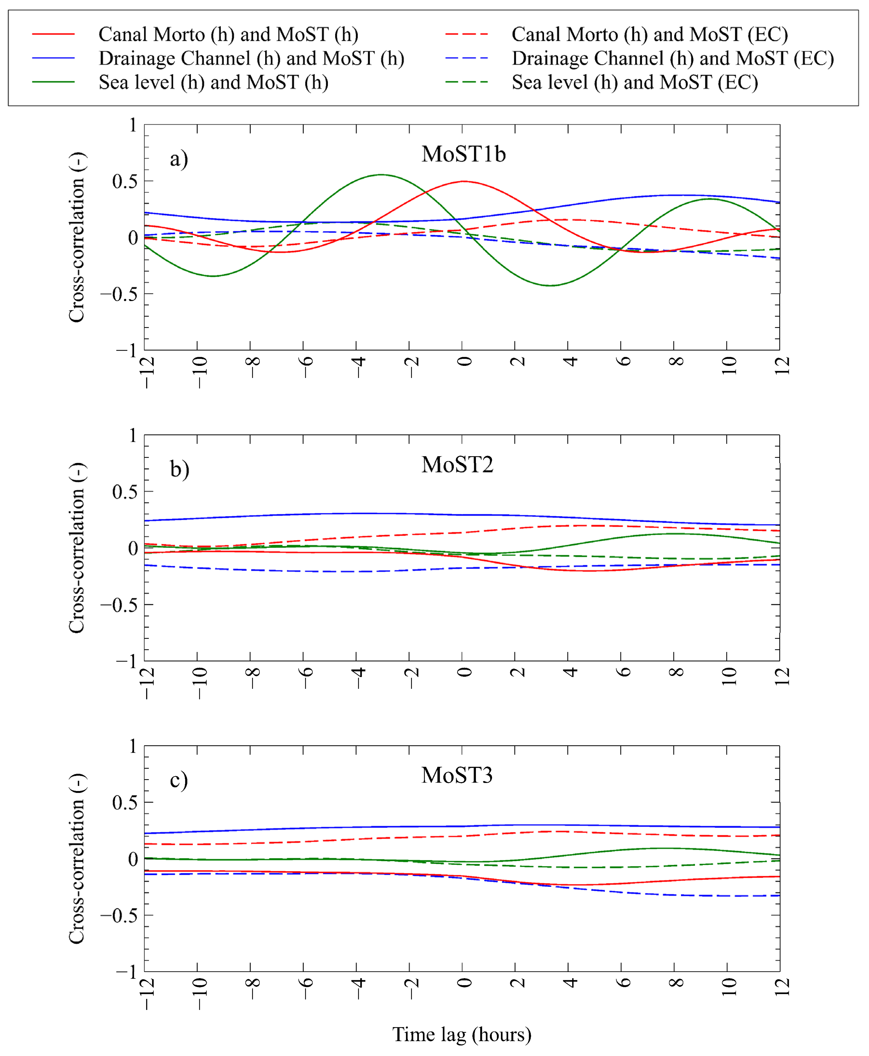
5.2.1. Phreatic Aquifer

The water table of the phreatic aquifer decreases southwards and from north to south with a difference of about 1 m, which is approximatively the same difference in the ground elevation of the farmlands. The aquifer shows background values of EC decreasing southward from 38 to 28 mS cm−1 at the top and from 40 to 33 mS cm−1 at the bottom, according to the increasing distance from the lagoon. In dry conditions, a clear EC stratification is shown only in the site MoST3, while it is quite homogeneous in MoST1b and MoST2.
The collected data, together with the cross-correlation analyses, support that both water levels and EC values in the aquifer, are related to the occurrence, often simultaneous, of several forcing factors such as atmospheric precipitations, tide encroachment, and water management from pumping station, all contributing to the complexity of the system response.
Major water table rises are concomitant to precipitations, which lead to significant EC decreases in the uppermost layer and sometimes in the whole aquifer thickness (Figure 15c). The heavier the events, the longer the decrease in groundwater EC, also with the contribution of the freshwater dispersions from the Brenta and Bacchiglione riverbeds. The increase of water table during rainfall events is generally rapid, often instantaneous, while the decrease in EC is differentiated from the northern and the southern sides of the studied area. The return to the normal conditions is generally quick in the northern part of the aquifer and slower in the southern ones.
EC and h values in the northern sector (MoST1b) are clearly driven by the tide at sea (Figure 15a) (in phase and delayed, 3 h and 4 h 40 min, respectively, with respect to the tidal signal), while they do not show a significant correlation in the southern sector (MoST2 and MoST3 sites), at least for short-term intervals (daily). This different behavior between the northern and the southern part of the aquifer should be explained taking into consideration their distance from the Venice lagoon and the Brenta and Bacchiglione rivers, whose terminal section, next to the river mouths, could be easily affected by salt wedge.
A correlation between the h of the aquifer and the water level of the CM has been observed. The h value is in phase with no delay next to the watercourse and in opposition to phase (4 h delay) in the farthest sector. The EC values in the aquifer correlate in phase 4h early with the CM water level both in the north and south sites (MoST1b, MoST2, and MoST3). This supports that mobile gates prevent the seawater from entering the CM just at the beginning of the tidal rise (Figure 15a).
The drainage channel levels (pumping station inflow) drive the phreatic aquifer levels in MoST2, while at MoST1b and MoST3, the aquifer anticipates in phase the water level of the drainage channel with respect to the aquifer level but shows different behaviors. Specifically, the results of cross-correlation analysis indicate that the drainage channel reaches maximum values after 8 h 20 min of the maximum h in the northern site (aquifer drives the drainage). Conversely, the drainage channel levels anticipate in phase h of about 3 h 40 min at MoST2 (drainage drives the aquifer). At MoST3 site, the h changes in phase with the drainage channel level and exhibits a max correlation with 2 h 20 min early (aquifer drives drainage). The time difference between north and south sectors is related to the distance between the piezometers and the drainage channel. The DC level is inversely correlated with the EC in the aquifer. In the northern site (MoST1b site), the EC leads the channel level but the maximum correlation is not reached within 12 h. In the south, the correlation shows different behavior, at MoST2 site EC is 4 h 30 min delayed and at MoST3 site EC is 10 h in advance. This is quite surprising, given the proximity of the two sites; we hypothesize that such difference is likely depending on the local variability of the subsoil architecture. Therefore, the pumping station drives the phreatic aquifer levels in MoST2, while at MoST1b and MoST3 sites the driver is the aquifer. The lowering of the drainage level, by the operation of the pumping station, causes an increase of the EC in the aquifer with different timing.
The EC changes in the aquifer during the examined dry period, even though in the range of a few mS cm−1, are significant. Being approximative with the same delay of the tide, it is reasonable to suppose that increasing EC values are influenced by the seawater intrusion from the lagoon basin and from the seawater encroachment along the Brenta and Bacchiglione rivers. Decreasing values, vice versa, are driven by the leakages from the watercourse beds when freshwater replaces the marine water towards the mouth at low tide. The contribution from the CM is excluded, or at least negligible, and limited to the proximity of the embankment in the very shallow subsoil (Figure 15b). The regulation gates at the CM mouth contrast the seawater propagation along the channel, maintaining freshwater in the upstream sections. During the closure of the gates, the water level in the CM rises, because of the freshwater accumulation upstream, but slower than the tide. After the opening of the gates, the levels of CM decreases following tide with almost the same timing. The leakage from the CM bed seems negligible as it should be of freshwater and the EC of the aquifer does not show any significant decrease when the regulation gates are closed (Figure 15a). The h and EC in the northern part of the aquifer (MoST1b) are not directly linked with levels of the CM, despite the significant cross-correlation. When EC rises, there is the concurrence of the following events: tidal rising and saltwater accumulation in the aquifer, GA closure and freshwater accumulation in CM. When tide lowers and gates open, EC decreases because of the Brenta–Bacchiglione system leaks freshwater in the aquifer (Figure 15a,b). Hence, the groundwater freshening is definitely not due to the influence of the CM.
In conclusion, the EC background of the phreatic aquifer is given by the seawater intrusion from the lagoon and the river mouths and is modulated by the exchanges with Brenta and Bacchiglione riverbeds especially during the ebb tide phase, while the leakage from CM is negligible.

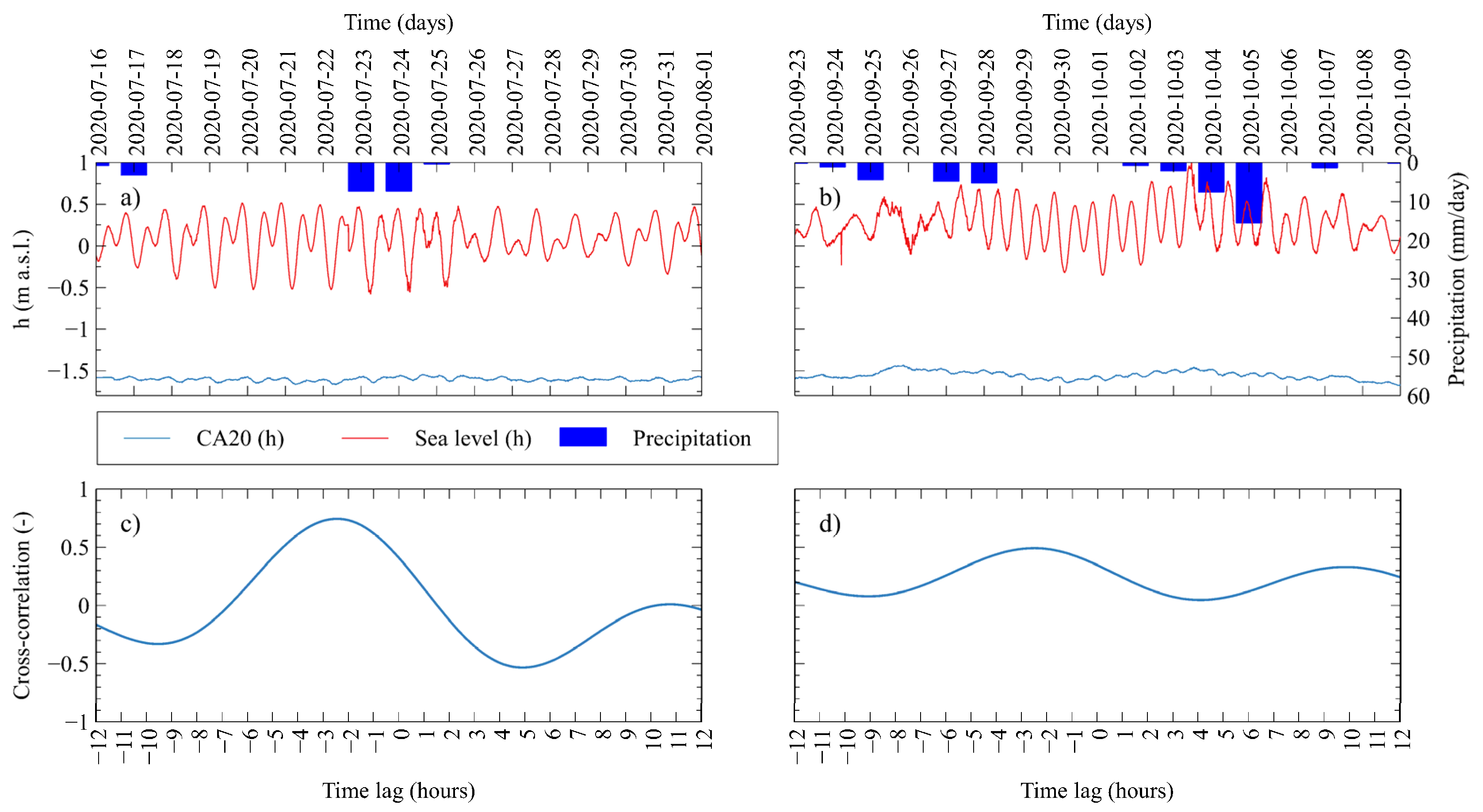
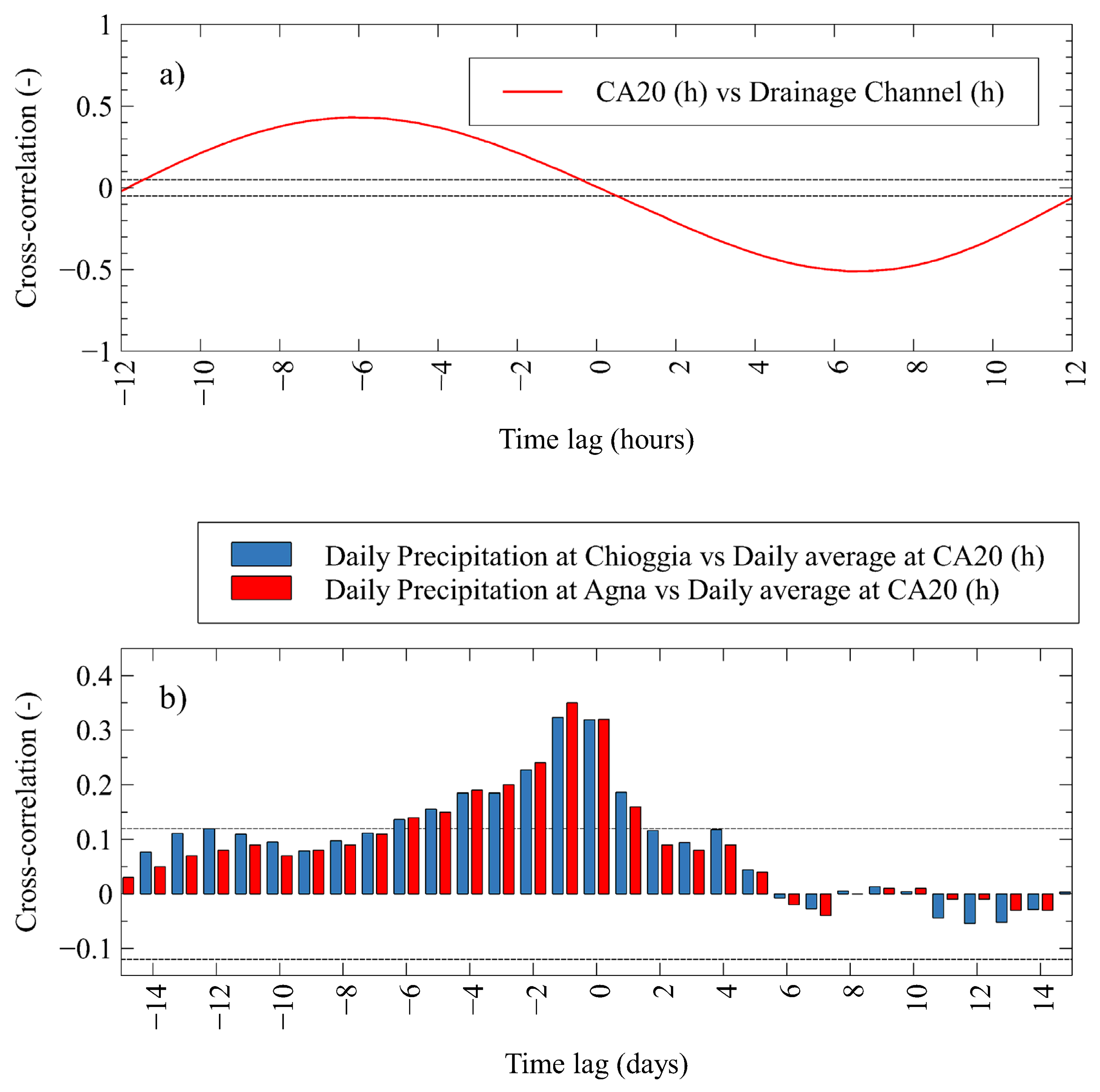
5.2.2. Confined Aquifer

Regarding the shallow confined aquifer, daily and fortnightly periods of sea level changes control the groundwater level, while they do not affect the salinity (Figure 15a,b). Daily changes of aquifer pressure are in phase with tidal cycle exhibiting a delay of 2 h 30 min. Maximum pressure generally occurs during spring tides (syzygy). Piezometer CA20 also follows in counterphase the level of the DC with a delay of 6 h 20 min (cross-correlation equals to 0.51). Regarding the relationship between precipitations and h changes, local precipitation leads to the rise of the groundwater level (Figure 15c) with maximum correlation in the same day, despite significant correlation up to the previous 5–6 days occurs. This suggests that the recharge zone of this aquifer is not far from the study area and in the order of 10 km.

6. Conclusions

The performed study demonstrates the capacity of the two monitoring systems customized and installed in the different locations and scales in successfully tackling the SWI processes and related consequences. The capability of two SWI monitoring systems has been demonstrated with emphasis to analyze and identify circumstances under which the SWI takes place within two coastal systems in the Adriatic Sea. The main outcomes of this study can be summarized as follows:
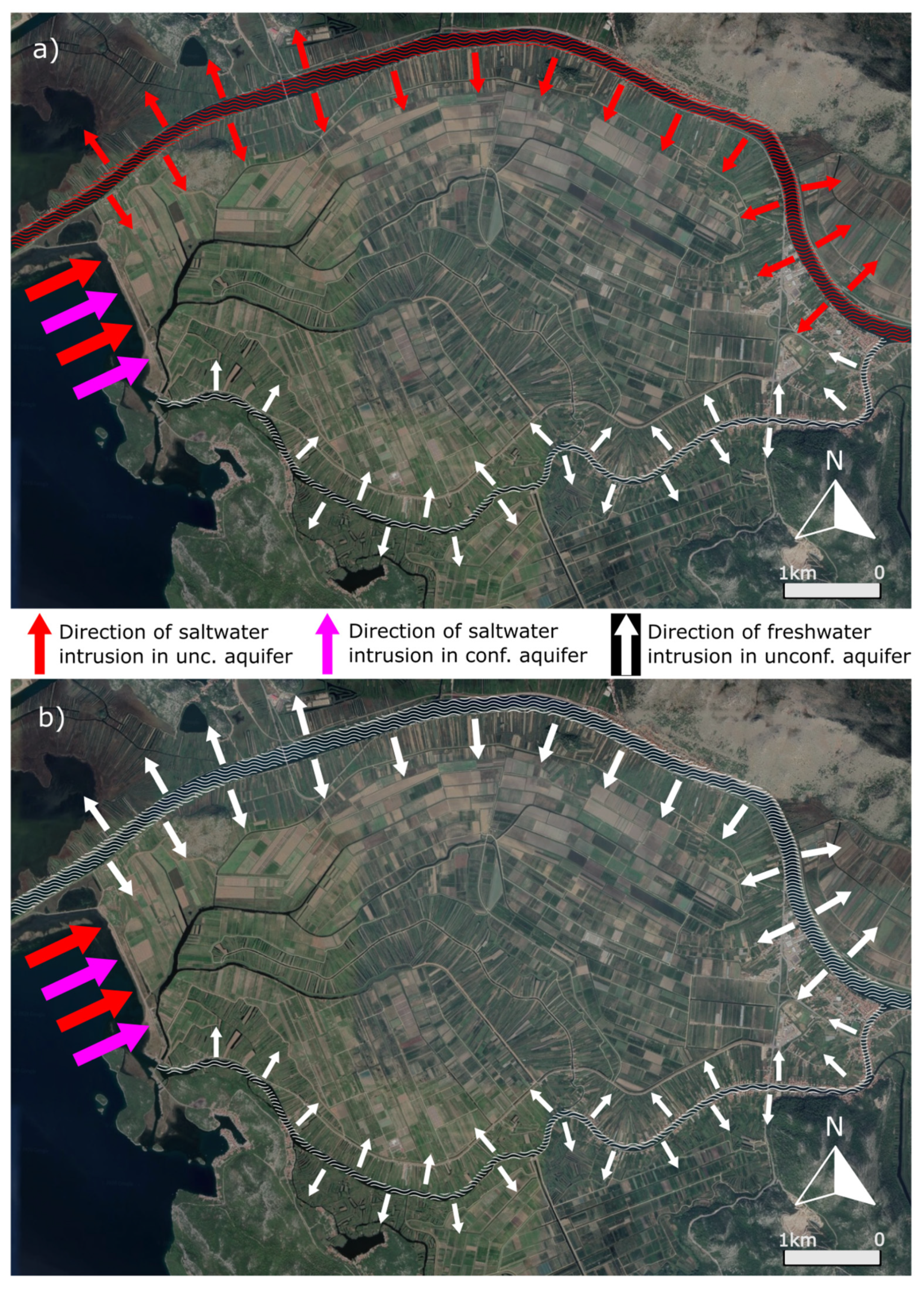
  • The Neretva Valley coastal system is shown to be dominantly influenced by the sea when dealing with salinity dynamics along the coastal area. The main saltwater inflow direction is from the sea. The confined aquifer seems to keep the salinity regime independently of the upper, unconfined aquifer. Contrarily to confined aquifer, an unconfined one is shown to be affected by the sea, artificial drainage, and external loadings.
  • During both rain and dry periods, confined aquifers keep constant EC values at all monitoring locations covered by the study, with almost negligible variations. This leads to a conclusion about the significant connection between this geological unit and the sea. Besides the EC, piezometric regime is shown to keep a frequency signature similar to that of the sea level.
  • Monitoring locations installed in the unconfined aquifer demonstrate fundamentally different behavior of groundwater features. The coastal area is dominantly controlled by the interplay of the sea and pumping station Modrič operative regime keeping the EC level around 50 mS cm−1 due to the active SWI. The central Valley area shows the influence of the river Neretva regime since the distance from P2 to river Neretva is approximately four times smaller than the sea distance from P2. This area is characterized by high EC values during the dry period while during the rain period, especially after the occurrence of intensive precipitation rates, EC is drastically decreased to approximately 10–15 mS cm−1. Vidrice area is a unique subsystem whose EC characteristic is increased during precipitation events. In the case of precipitation depths greater than 40 mm day−1, strict EC decrease is identified. To elaborate this in a comprehensive way, additional in situ observations, either the extension of the existing monitoring system has to be done.
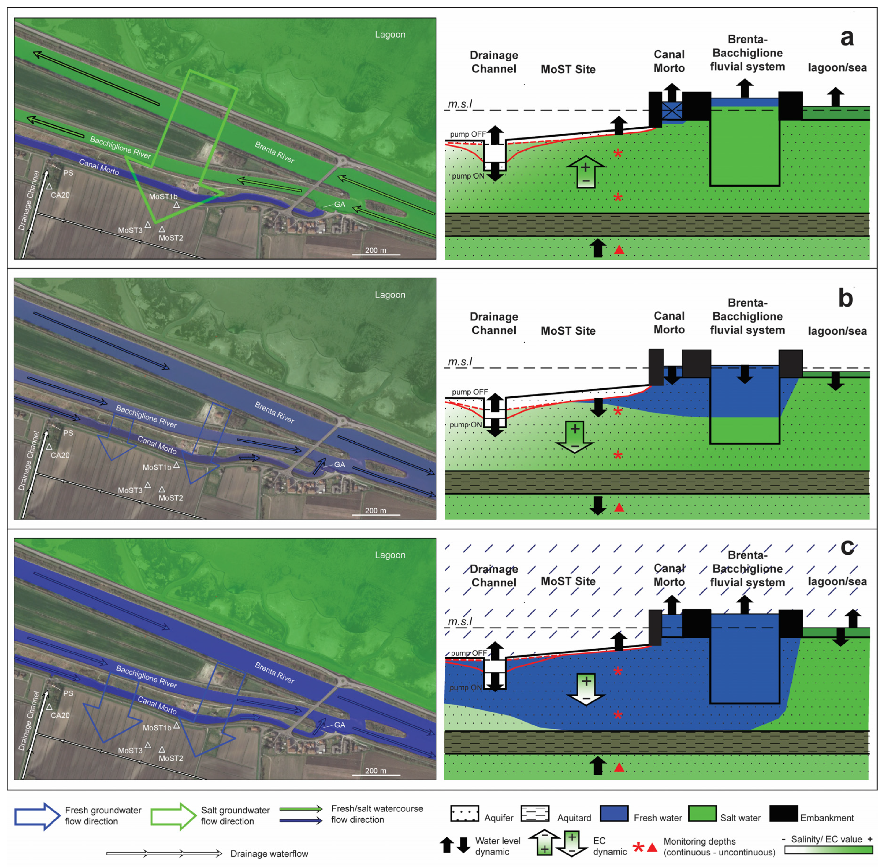
  • In the Venice site, the artificial drainage seasonally constrains the water table levels on the basis of the farmland activities. The rainfall events significantly mitigate the relevant high background of saltwater contamination in the aquifers. Since the almost constant high salinity background, the salinity intake from the Brenta and Bacchiglione river beds during the encroachment phase has been much more important than the dilution effect given by their freshwater outflows during low tides. As for the CM, the tidal regulation gates hamper the seawater encroachment during high sea levels and keep freshwater storage in the last stretch of the watercourse. However, the dispersion of the freshwater from the CM does not seem enough to significantly mitigate the salt background in the aquifer system;
  • Different locations show specific nature of the SWI parameters like temperature and EC;
  • The established monitoring systems enable the identification of processes influencing SWI.
The results of this comparative study allowed a better understanding of the groundwater dynamics and their driving forces. They will help in future management and planning of possible solutions for the mitigation of salt contamination in the highly valuable coastal farmlands of the two sites. Longer time series of data as well as further investigations, including time-lapse geoelectrical prospecting and chemical analysis of the waters, are necessary to fully comprehend the complexity of the continental–marine water exchanges both in the Neretva and Venice coastal aquifers.

Author Contributions

Conceptualization, V.S. and L.T.; methodology, I.L., L.T., A.B., and V.S.; software, A.B. and I.L.; validation, I.L., J.E., D.H., S.D., C.C., and A.B.; formal analysis, I.L., L.T., A.B., C.C., S.D., and V.S; investigation, I.L., V.S., J.E., L.T., A.B., C.C., S.D., and L.Z.; writing—original draft preparation, I.L., V.S., D.H., J.E., L.T., A.B., C.C., S.D., and L.Z.; writing—review and editing, I.L., V.S., D.H., J.E., L.T., A.B., C.C., S.D., and L.Z.; visualization, I.L. and C.C.; supervision, L.T. and V.S. All authors have read and agreed to the published version of the manuscript.

Funding

This research is funded by the contribution from the EU co-financing and the Interreg Italy-Croatia CBC Programme 2014–2020 (Priority Axes: Safety and Resilience) through the European Regional Development Fund as a part of project Monitoring Sea-water intrusion in coastal aquifers and Testing pilot projects for its mitigation (MoST) (AID: 10047742). Moreover, the research in the Croatian site was partially supported through project Monitoring of water and soil salinity for the Neretva valley area—project period 2019–2023. Funded by national water management agency Croatian water.

Institutional Review Board Statement

Not applicable.

Informed Consent Statement

Not applicable.

Data Availability Statement

Data sets available on request.

Acknowledgments

Authors are grateful to Marin Milin and Marko Džaja from Higra LTD for their valuable input and expertise in the monitoring system.

Conflicts of Interest

The authors declare no conflict of interest.

References

  1. Racetin, I.; Krtalic, A.; Srzic, V.; Zovko, M. Characterization of short-term salinity fluctuations in the Neretva River Delta situated in the southern Adriatic Croatia using Landsat-5 TM. Ecol. Indic. 2020, 110, 105924. [Google Scholar] [CrossRef]
  2. Sherif, M.M.; Singh, V.P. Effect of climate change on sea water intrusion in coastal aquifers. Hydrol. Process. 1999, 13, 1277–1287. [Google Scholar] [CrossRef]
  3. Sithara, S.; Pramada, S.K.; Thampi, S.G. Impact of projected climate change on seawater intrusion on a regional coastal aquifer. J. Earth Syst. Sci. 2020, 129. [Google Scholar] [CrossRef]
  4. van Engelen, J.; Verkaik, J.; King, J.; Nofal, E.R.; Bierkens, M.F.P.; Oude Essink, G.H.P. A three-dimensional palaeohydrogeological reconstruction of the groundwater salinity distribution in the Nile Delta Aquifer. Hydrol. Earth Syst. Sci. 2019, 23, 5175–5198. [Google Scholar] [CrossRef] [Green Version]
  5. Paldor, A.; Shalev, E.; Katz, O.; Aharonov, E. Dynamics of saltwater intrusion and submarine groundwater discharge in confined coastal aquifers: A case study in northern Israel. Hydrogeol. J. 2019, 27, 1611–1625. [Google Scholar] [CrossRef]
  6. Stein, S.; Yechieli, Y.; Shalev, E.; Kasher, R.; Sivan, O. The effect of pumping saline groundwater for desalination on the fresh-saline water interface dynamics. Water Res. 2019, 156, 46–57. [Google Scholar] [CrossRef] [PubMed]
  7. Goswami, R.R.; Clement, T.P. Laboratory-scale investigation of saltwater intrusion dynamics. Water Resour. Res. 2007, 43. [Google Scholar] [CrossRef]
  8. Memari, S.S.; Bedekar, V.S.; Clement, T.P. Laboratory and Numerical Investigation of Saltwater Intrusion Processes in a Circular Island Aquifer. Water Resour. Res. 2020, 56. [Google Scholar] [CrossRef]
  9. Nguyen, T.T.M.; Yu, X.; Pu, L.; Xin, P.; Zhang, C.; Barry, D.A.; Li, L. Effects of Temperature on Tidally Influenced Coastal Unconfined Aquifers. Water Resour. Res. 2020, 56, e2019WR026660. [Google Scholar] [CrossRef]
  10. Nepal, C.M.; Vijay, P.S.; Somvir, S.; Vijay, S.S. Hydrochemical characteristic of coastal aquifer from Tuticorin, Tamil Nadu, India. Environ. Monit. Assess. 2011, 175, 531–550. [Google Scholar] [CrossRef]
  11. Fadili, A.; Najib, S.; Mehdi, K.; Riss, J.; Malaurent, P.; Makan, A. Geoelectrical and hydrochemical study for the assessment of seawater intrusion evolution in coastal aquifers of Oualidia, Morocco. J. Appl. Geophys. 2017, 146, 178–187. [Google Scholar] [CrossRef]
  12. Levanon, E.; Yechieli, Y.; Shalev, E.; Friedman, V.; Gvirtzman, H. Reliable monitoring of the transition zone between fresh and saline waters in coastal aquifers. Groundw. Monit. Remediat. 2013, 33, 101–110. [Google Scholar] [CrossRef]
  13. Kim, J.H.; Lee, J.; Cheong, T.J.; Kim, R.H.; Koh, D.C.; Ryu, J.S.; Chang, H.W. Use of time series analysis for the identification of tidal effect on groundwater in the coastal area of Kimje, Korea. J. Hydrol. 2005, 300, 188–198. [Google Scholar] [CrossRef]
  14. Kim, K.Y.; Park, Y.S.; Kim, G.P.; Park, K.H. Dynamic freshwater-saline water interaction in the coastal zone of Jeju Island, South Korea. Hydrogeol. J. 2009, 17, 617–629. [Google Scholar] [CrossRef]
  15. Kim, K.Y.; Chon, C.M.; Park, K.H. A simple method for locating the fresh water-salt water interface using pressure data. Ground Water 2007, 45, 723–728. [Google Scholar] [CrossRef] [PubMed]
  16. Kue-Young, K.; Chul-Min, C.; Ki-Hwa, P.; Yun-Seok, P.; Nam-Chil, W. Multi-depth monitoring of electrical conductivity and temperature of groundwater at a multilayered coastal aquifer: Jeju Island, Korea. Hydrol. Process. 2008, 22, 3724–3733. [Google Scholar] [CrossRef]
  17. Yang, H.; Shimada, J.; Shibata, T.; Okumura, A.; Pinti, D.L. Freshwater lens oscillation induced by sea tides and variable rainfall at the uplifted atoll island of Minami-Daito, Japan. Hydrogeol. J. 2020, 28, 2105–2114. [Google Scholar] [CrossRef]
  18. Srzić, V.; Lovrinović, I.; Racetin, I.; Pletikosić, F. Hydrogeological Characterization of Coastal Aquifer on the Basis of Observed Sea Level and Groundwater Level Fluctuations: Neretva Valley Aquifer, Croatia. Water 2020, 12, 348. [Google Scholar] [CrossRef] [Green Version]
  19. Krvavica, N.; Ružić, I. Estuarine, Coastal and Shelf Science Assessment of sea-level rise impacts on salt-wedge intrusion in idealized and Neretva River Estuary. Estuar. Coast. Shelf Sci. 2020, 234, 106638. [Google Scholar] [CrossRef] [Green Version]
  20. Romić, D.; Castrignanò, A.; Romić, M.; Buttafuoco, G.; Bubalo Kovačić, M.; Ondrašek, G.; Zovko, M. Modelling spatial and temporal variability of water quality from different monitoring stations using mixed effects model theory. Sci. Total Environ. 2020, 704, 135875. [Google Scholar] [CrossRef] [PubMed]
  21. Zovko, M.; Romi, D.; Colombo, C.; Di, E.; Romi, M.; Buttafuoco, G.; Castrignanò, A. Geoderma A geostatistical Vis-NIR spectroscopy index to assess the incipient soil salinization in the Neretva River valley, Croatia. Geoderma 2018, 332, 60–72. [Google Scholar] [CrossRef]
  22. Carbognin, L.; Tosi, L. Interaction between Climate Changes, Eustacy and Land Subsidence in the North Adriatic Region, Italy. Mar. Ecol. 2002, 23, 38–50. [Google Scholar] [CrossRef]
  23. Tosi, L.; Da Lio, C.; Strozzi, T.; Teatini, P. Combining L- and X-Band SAR Interferometry to Assess Ground Displacements in Heterogeneous Coastal Environments: The Po River Delta and Venice Lagoon, Italy. Remote Sens. 2016, 8. [Google Scholar] [CrossRef] [Green Version]
  24. Benvenuti, G.; Norinelli, A.; Zambrano, R. Contributo alla conoscenza del sottosuolo dell’area circumlagunare veneta mediante sondaggi elettrici verticali. Boll. Geofis. Teor. Appl. 1973, 15, 23–38. [Google Scholar]
  25. Di Sipio, E.; Galgaro, A.; Zuppi, G.M. New geophysical knowledge of groundwater systems in Venice estuarine environment. Estuar. Coast. Shelf Sci. 2006, 66, 6–12. [Google Scholar] [CrossRef]
  26. Rapaglia, J. Submarine groundwater discharge into Venice Lagoon, Italy. Estuaries 2005, 28, 705–713. [Google Scholar] [CrossRef]
  27. Gattacceca, J.C.; Vallet-Coulomb, C.; Mayer, A.; Claude, C.; Radakovitch, O.; Conchetto, E.; Hamelin, B. Isotopic and geochemical characterization of salinization in the shallow aquifers of a reclaimed subsiding zone: The southern Venice Lagoon coastland. J. Hydrol. 2009, 378, 46–61. [Google Scholar] [CrossRef]
  28. Teatini, P.; Tosi, L.; Viezzoli, A.; Baradello, L.; Zecchin, M.; Silvestri, S. Understanding the hydrogeology of the Venice Lagoon subsurface with airborne electromagnetics. J. Hydrol. 2011, 411, 342–354. [Google Scholar] [CrossRef]
  29. Viezzoli, A.; Tosi, L.; Teatini, P.; Silvestri, S. Surface water-groundwater exchange in transitional coastal environments by airborne electromagnetics: The Venice Lagoon example. Geophys. Res. Lett. 2010, 37. [Google Scholar] [CrossRef]
  30. De Franco, R.; Biella, G.; Tosi, L.; Teatini, P.; Lozej, A.; Chiozzotto, B.; Giada, M.; Rizzetto, F. Monitoring the saltwater intrusion by time lapse electrical resistivity tomography: The Chioggia test site (Venice Lagoon, Italy). J. Appl. Geophys. 2009, 69, 117–130. [Google Scholar] [CrossRef]
  31. Da Lio, C.; Carol, E.; Kruse, E.; Teatini, P.; Tosi, L. Saltwater contamination in the managed low-lying farmland of the Venice coast, Italy: An assessment of vulnerability. Sci. Total Environ. 2015, 533, 356–369. [Google Scholar] [CrossRef] [PubMed]
  32. Faculty of Civil Engineering. Water Management Solution and Arrangement of the Lower Neretva Basin; Faculty of Civil Engineering: Split, Croatia, 1996. [Google Scholar]
  33. Hrvatske Vode. Provedbeni Plan Obrane od Poplava Branjenog Područja Sektor F—Južni Jadran Branjeno Područje 32: Područja Malih Slivova Neretva—Korčula i Dubrovačko Primorje i Otoci; Hrvatske Vode: Zagreb, Croatia, 2014. [Google Scholar]
  34. Geoid-Beroš Ltd. Piezometer Drilling for Purpose of Groundwater Monitoring System; Geoid-Beroš Ltd.: Jalkovec, Croatia, 2014. [Google Scholar]
  35. Institute IGH PLC. Monitoring Sea-Water Intrusion in Coastal Aquifers and Testing Pilot Projects for Its Mitigation; Geophysical Investigation Report; Institute IGH PLC: Zagreb, Croatia, 2019. [Google Scholar]
  36. Elektrosond. Hydrogeological Investigation Works Opuzen—Mouth of Neretva; Elektrosond: Zagreb, Croatia, 1963. [Google Scholar]
  37. Geofizika. Geophysical Investigations/Geoelectrical and Seismic/at Opuzen—Mouth of Neretva; Geofizika: Zagreb, Croatia, 1962. [Google Scholar]
  38. GEOKON. Drilling Report of Two Pairs of Piezometers Downstream of the Neretva River; GEOKON: Zagreb, Croatia, 2005. [Google Scholar]
  39. GEOKON. Geotechnical Investigation Works for Irrigation System Conceptual Design Downstream of the Neretva River; GEOKON: Zagreb, Croatia, 2008. [Google Scholar]
  40. GEOKON. No Geotechnical Investigation Works for Siphon below Mala Neretva at the Pumping Station Prag (Vidrice); GEOKON: Zagreb, Croatia, 2013. [Google Scholar]
  41. Geofizika. Water Investigation Works at Opuzen—Šetka; Geofizika: Zagreb, Croatia, 1966. [Google Scholar]
  42. Institute IGH PLC. Geotechnical Study for Irrigation System Subsystem Opuzen (Phases A and J); Institute IGH PLC: Zagreb, Croatia, 2013. [Google Scholar]
  43. Tosi, L.; Teatini, P.; Brancolini, G.; Zecchin, M.; Carbognin, L.; Affatato, A.; Baradello, L. Three-dimensional analysis of the Plio-Pleistocene seismic sequences in the Venice Lagoon (Italy). J. Geol. Soc. 2012, 169, 507–510. [Google Scholar] [CrossRef]
  44. Zecchin, M.; Tosi, L. Multi-sourced depositional sequences in the Neogene to Quaternary succession of the Venice area (northern Italy). Mar. Pet. Geol. 2014, 56, 1–15. [Google Scholar] [CrossRef]
  45. Donnici, S.; Serandrei-Barbero, R.; Bini, C.; Bonardi, M.; Lezziero, A. The Caranto Paleosol and Its Role in the Early Urbanization of Venice. Geoarchaeology 2011, 26, 514–543. [Google Scholar] [CrossRef]
  46. Gasparetto-Stori, G.; Strozzi, T.; Teatini, P.; Tosi, L.; Vianello, A.; Wegmüller, U. Dem of the Veneto Plain by Ers2-Envisat Cross-Interferometry. In Proceedings of the 7th EUREGEO European Congress on Regional Geoscientific Cartography and Information Systems, Bologna, Italy, 12–15 June 2012. [Google Scholar]
  47. Tosi, L.; Rizzetto, F.; Bonardi, M.; Donnici, S.; Serandrei Barbero, R.T. Chioggia-Malamocco. In Note Illustrative della Carta Geologica d’Italia alla Scala 1:50.000; SystemCart: Rome, Italy, 2007; pp. 148–149. [Google Scholar]
  48. Tosi, L.; Rizzetto, F.; Zecchin, M.; Brancolini, G.; Baradello, L. Morphostratigraphic framework of the Venice Lagoon (Italy) by very shallow water VHRS surveys: Evidence of radical changes triggered by human-induced river diversions. Geophys. Res. Lett. 2009, 36. [Google Scholar] [CrossRef]
  49. Zecchin, M.; Brancolini, G.; Tosi, L.; Rizzetto, F.; Caffau, M.; Baradello, L. Anatomy of the Holocene succession of the southern Venice lagoon revealed by very high-resolution seismic data. Cont. Shelf Res. 2009, 29, 1343–1359. [Google Scholar] [CrossRef]
  50. Vallejos, A.; Sola, F.; Pulido-Bosch, A. Processes Influencing Groundwater Level and the Freshwater-Saltwater Interface in a Coastal Aquifer. Water Resour. Manag. 2014, 29, 679–697. [Google Scholar] [CrossRef]
  51. Proakis, J.G.; Manolakis, D.G. Digital Signal Processing, 4th ed.; Prentice-Hall, Inc.: Upper Saddle River, NJ, USA, 2006; ISBN 9788578110796. [Google Scholar]
  52. Cerna, M.; Harvey, A.F. The Fundamentals of FFT-Based Signal Analysis and Measurement; Application Note 041; National Instruments: Austin, TX, USA, 2000. [Google Scholar]
  53. Turnadge, C.; Crosbie, R.S.; Barron, O.; Rau, G.C. Comparing Methods of Barometric Efficiency Characterization for Specific Storage Estimation. Groundwater 2019, 57, 844–859. [Google Scholar] [CrossRef]
  54. Fuentes-Arreazola, M.A.; Ramírez-Hernández, J.; Vázquez-González, R. Hydrogeological properties estimation from groundwater level natural fluctuations analysis as a low-cost tool for the Mexicali Valley Aquifer. Water 2018, 10. [Google Scholar] [CrossRef] [Green Version]
  55. Dong, L.; Shimada, J.; Kagabu, M.; Yang, H. Barometric and tidal-induced aquifer water level fluctuation near the Ariake Sea. Environ. Monit. Assess. 2015, 187. [Google Scholar] [CrossRef]
  56. Merritt, M.L. Estimating Hydraulic Properties of the Floridan Aquifer System by Analysis of Earth-Tide, Ocean-Tide, and Barometric Effects, Collier and Hendry Counties, Florida; U.S. Geological Survey: Reston, VA, USA, 2004. [Google Scholar]
  57. Levanon, E.; Yechieli, Y.; Gvirtzman, H.; Shalev, E. Tide-induced fluctuations of salinity and groundwater level in unconfined aquifers—Field measurements and numerical model. J. Hydrol. 2017, 551, 665–675. [Google Scholar] [CrossRef]
  58. Jiao, J.J.; Tang, Z. An analytical solution of groundwater response to tidal fluctuation in a leaky confined aquifer. Water Resour. Res. 1999, 35, 747–751. [Google Scholar] [CrossRef] [Green Version]
  59. Dong, L.; Chen, J.; Fu, C.; Jiang, H. Analysis of groundwater-level fluctuation in a coastal confined aquifer induced by sea-level variation. Hydrogeol. J. 2012, 20, 719–726. [Google Scholar] [CrossRef]
  60. Kim, K.Y.; Seong, H.; Kim, T.; Park, K.H.; Woo, N.C.; Park, Y.S.; Koh, G.W.; Park, W.B. Tidal effects on variations of fresh-saltwater interface and groundwater flow in a multilayered coastal aquifer on a volcanic island (Jeju Island, Korea). J. Hydrol. 2006, 330, 525–542. [Google Scholar] [CrossRef]
  61. Ferla, M.; Cordella, M.; Michielli, L.; Rusconi, A. Long-term variations on sea level and tidal regime in the lagoon of Venice. Estuar. Coast. Shelf Sci. 2007, 75, 214–222. [Google Scholar] [CrossRef]
  62. Lovrinović, I.; Srzić, V.; Vranješ, M.; Džaja, M. Coastal aquifer characteristics determination based on in-situ observations: River Neretva Valley Aquifer. In Proceedings of the European Water Resources Association (EWRA), General Assembly, Madrid, Spain, 25–29 June 2019. [Google Scholar]
  63. Lovrinović, I.; Srzić, V.; Matić, I.; Krnić, P. Multi component analysis of processes controlling seawater intrusion dynamics in Neretva delta area. In Proceedings of the AGU—American Geoscience Union, New Orleans, LA, USA, 1–17 December 2020. [Google Scholar]
  64. McMillan, T.C.; Rau, G.C.; Timms, W.A.; Andersen, M.S. Utilizing the Impact of Earth and Atmospheric Tides on Groundwater Systems: A Review Reveals the Future Potential. Rev. Geophys. 2019, 57, 281–315. [Google Scholar] [CrossRef] [Green Version]
  65. Rahi, K.A.; Halihan, T. Identifying aquifer type in fractured rock aquifers using harmonic analysis. Groundwater 2013, 51, 76–82. [Google Scholar] [CrossRef]
  66. Faculty of Civil Engineering, Geodesy and Architecture, University of Split. Salinity Monitoring at Lower Neretva Area—Report for the Year 2020; Faculty of Civil Engineering, Geodesy and Architecture, University of Split: Split, Croatia, 2020. [Google Scholar]
  67. Badaruddin, S.; Werner, A.D.; Morgan, L.K. Water table salinization due to seawater intrusion. Water Resour. Res. 2015, 51, 8397–8408. [Google Scholar] [CrossRef]
Figure 1. River Neretva valley area of interest with locations of boreholes, observation piezometers, surface water gauges, and geological profiles.
Water 13 00561 g001
Figure 2. Geological cross-sections 1-1 and 2-2 of the River Neretva valley.
Water 13 00561 g002
Figure 3. The southern Venice lagoon—coastal area test site with the location of the piezometers (MoST1b, MoST2, MoST3, and CA20), the monitoring points of the surface water levels of the drainage channel (DC) controlled by the pumping station (PS), and the Canal Morto (CM). SA and AG are the locations of meteorological stations, Sant’ Anna and Agna, respectively, while Chioggia tide gauge station is denoted by TG and GA indicates gates at CM.
Water 13 00561 g003
Figure 4. Hydrogeological setting of the upper Pleistocene and Holocene depositional units.
Water 13 00561 g004
Figure 5. Observed time series from Neretva valley coastal aquifer system: (a) h in confined aquifer D1, h, T and electrical conductivity (EC) in unconfined aquifer P1, sea level and precipitation during February 2019; (b) h in confined aquifer P1, h, T and EC in unconfined aquifer P1, sea level and precipitation during July 2019; (c) h in confined aquifer D2, h, T and EC in unconfined aquifer P2, sea level, river surface elevation and precipitation during February 2019; (d) h in confined aquifer D2, h, T and EC in unconfined aquifer P2, sea level, river surface elevation and precipitation during July 2019; (e) h in confined aquifer D4, h, T and EC in unconfined aquifer P4, sea level, river surface elevation, OUN h and UUU h and precipitation during February 2019; (f) h in confined aquifer D4, h, T and EC in unconfined aquifer P4, sea level, river surface elevation, OUN and UUU h and precipitation during July 2019.
Water 13 00561 g005
Figure 6. Analysis of observed time series: (a) Amplitude spectral density (ASD) for sea level and piezometric head D1, D2, and D4—February 2019; (b) cross-correlation functions for sea level and piezometric head D1, D2, and D4—February 2019; (c) Amplitude spectral density (AD) for sea level and piezometric head D1, D2, and D4—July 2019; (d) cross-correlation functions for sea level and piezometric head D1, D2, and D4—July 2019.
Water 13 00561 g006
Figure 7. Cross-correlation functions determined for February and July 2019: (a) Sea level—h and sea level—EC cross-correlation functions for P1; (b) h and EC cross-correlation functions for P2 and (c) h and EC cross-correlation functions for P4.
Water 13 00561 g007
Figure 8. Time series of forcing factors of the aquifer dynamics in the southern Venice Lagoon during the period July 16th–October 22nd: Daily precipitation from SA meteorological station, Sea level observed at TG; CM water level (PS outflow) and DC h (PS inflow).
Water 13 00561 g008
Figure 9. Groundwater dynamics of the unconfined aquifer in the period July 16th–October 22nd. EC and T detected at the top and the bottom of the aquifer: (a) piezometer MoST1b at −3.94 and −6.48 m a.s.l.; (b) piezometer MoST2 at −4.11; and −7.83 m a.s.l.; and (c) piezometer MoST3 at −4.03 and −10.52 m a.s.l.
Water 13 00561 g009
Figure 10. Cross-correlation functions determined for the period 2–19 September 2020: (a) piezometer MoST1b; (b) piezometer MoST2; and (c) piezometer MoST3.
Water 13 00561 g010
Figure 11. (a) Measurements taken at piezometer CA20 compared with the sea level data recorded at the Chioggia tide gauge station and daily precipitation at Sant’Anna (SA); (b) resulting amplitude spectral density (ASD) from the Fourier analyses applied to the pressure signal recorded in Chioggia tide gauge station; and (c) CA20 h amplitude spectral density (ASD).
Water 13 00561 g011
Figure 12. Detailed short-term analysis for (a) 16 July 2020 10:00am–01 August 2020 09:50am and (b) 23 September 2020 03:00pm–09 October 2020 08:00am; (c) and (d) are the cross-correlation between sea level and CA20 piezometric head over the two short periods.
Water 13 00561 g012
Figure 13. (a) DC level and CA20 h cross-correlation over the time span 16th July–1st August (2303 values); (b) Cross-correlation functions between daily precipitation in the close neighbors (SA and AG) and CA20 water level over the period 31 January 2020 to 10 November 2020.
Water 13 00561 g013
Figure 14. Conceptual definition of the Neretva Valley area sea water intrusion (SWI) pathways: (a) summer (dry) period; (b) winter (rain) period.
Water 13 00561 g014
Figure 15. Schematic representation of the SWI and freshwater pathways, obtained over the monitoring period July–October 2020, in three different scenarios: (a) dry periods with high tide and CM gate closed; (b) dry periods with low tide and CM gate opened; and (c) wet periods with heavy precipitations (regardless of high or low tide and gate closed or opened).
Water 13 00561 g015
Table 1. Summary of the characteristic of the monitoring piezometers at the Venice coastal aquifer site.
PiezometerGround Level
(m a.s.l.)
Screen Section
(m a.s.l.)
Upper Sensor Depth
(m a.s.l.)
Lower Sensor Depth
(m a.s.l.)
Observed Variables
MoST1b−1.73−2.73 to −11.73−3.94−6.48P, EC, T
MoST2−2.51−3.71 to −11.91−4.11−7.83P, EC, T
MoST3−2.35−3.55 to −12.05−4.03−10.52P, EC, T
CA20−1.94−16.94 to −21.94−2.89P
Table 2. Harmonic constituent variables for sea level and piezometric head signals in D1, D2, and D4 for period of February and July 2019.
2019FebruaryJuly
Sea Level
ConstituentsO1K1M2S2O1K1M2S2
Amplitude (m)0.0370.0610.0900.0680.0290.1080.0850.043
Period (h)25.8524.0012.4412.0025.8524.0012.4412.00
Phase (°)24.541.4920.43−113.46−167.61149.93−32.46−103.00
D1
ConstituentsO1K1M2S2O1K1M2S2
Amplitude (m)0.0180.0470.0470.0370.0180.0620.0460.023
Period (h)25.8524.0012.4412.0025.8524.0012.4412.00
Phase (°)−7.84−32.23−5.80−128.43160.36127.32−55.51−124.96
D2
ConstituentsO1K1M2S2O1K1M2S2
Amplitude (m)0.0140.0400.0260.0190.0140.0420.0270.012
Period (h)25.8524.0012.4412.0025.8524.0012.4412.00
Phase (°)−40.10−41.67−32.33−148.18129.6698.92−92.03−158.43
D4
ConstituentsO1K1M2S2O1K1M2S2
Amplitude (m)0.0130.0320.0150.0080.0110.0290.0120.006
Period (h)25.8524.0012.4412.0025.8524.0012.4412.00
Phase (°)−68.10−79.93−85.65154.6691.6453.48−158.64138.56
Publisher’s Note: MDPI stays neutral with regard to jurisdictional claims in published maps and institutional affiliations.

