Trend Analyses of Baseflow and BFI for Undisturbed Watersheds in Michigan—Constraints from Multi-Objective Optimization

Abstract

Documenting how ground- and surface water systems respond to climate change is crucial to understanding water resources, particularly in the U.S. Great Lakes region, where drastic temperature and precipitation changes are observed. This study presents baseflow and baseflow index (BFI) trend analyses for 10 undisturbed watersheds in Michigan using (1) multi-objective optimization (MOO) and (2) modified Mann–Kendall (MK) tests corrected for short-term autocorrelation (STA). Results indicate a variability in mean baseflow (0.09–8.70 m³/s) and BFI (67.9–89.7%) that complicates regional-scale extrapolations of groundwater recharge. Long-term (>60 years) MK trend tests indicate a significant control of total precipitation (P) and snow- to rainfall transitions on baseflow and BFI. In the Lower Peninsula Rifle River watershed, increasing P and a transition from snow- to rainfall has increased baseflow at a lower rate than streamflow; an overall pattern that may contribute to documented flood frequency increases. In the Upper Peninsula Ford River watershed, decreasing P and a transition from rain- to snowfall had no significant effects on baseflow and BFI. Our results highlight the value of an objectively constrained BFI parameter for shorter-term (<50 years) hydrologic trend analysis because of a lower STA susceptibility.

1. Introduction

Considered to be in the “bullseye” of climate change, watersheds in the U.S. Great Lakes Basin, and in the state of Michigan in particular, have undergone dramatic hydrologic transformations [1]. Despite the documented increases in temperature and extreme precipitation events [2,3,4], resulting effects on water balance parameters (e.g., total precipitation, evapotranspiration, groundwater recharge) have shown to be highly complex [4,5,6,7,8], as evidenced by the spatiotemporal variability of precipitation, streamflow, groundwater, and lake level trends [5,8,9,10]. Of the hydro-climate time series data used for trend evaluations of water balance parameters, baseflow (defined as the streamflow component sourced from groundwater) is usually not included. This likely reflects the uncertainty associated with the various estimation procedures [11,12] or data shortage from unregulated/undisturbed watersheds [7,13,14]. Nevertheless, baseflow constraints are of key importance in the assessment of water quality and stream biodiversity in droughts [15,16,17,18,19,20,21,22], as well as in the calibration of hydrologic models of groundwater recharge [6,23,24,25,26]. Moreover, a comparison of the concurrent trends of hydrograph components through the baseflow index (BFI = ratio of mean baseflow over mean streamflow) allows for an assessment of the relative impacts of climatic stressors on groundwater and surface water resources.

Baseflow is commonly estimated from streamflow records using hydrograph separation techniques such as graphical-, recession-curve-, chemical mass balance (CMB)-, and/or recursive digital filter (RDF)-based methods. Although widely accepted, each of these methods relies on subjective input parameters such as the choice of algorithm to draw connecting lines in the streamflow hydrograph [27,28,29], the distinction of recession periods [30,31], the selection of appropriate groundwater and surface runoff end-member chemistries [18,32,33], or the choice of filter parameters in the RDF methods [11,34,35,36]. While some guidance exists for method implementation and choice of input parameters based on hydrogeologic regime and data availability [29,34,36,37,38], uncertainty is generally not addressed based on the informed choice of input parameter range applicable to a specific setting, but rather through the use of multiple methods run on default parameters [11,12,25,36].

A recent study [39] presented a new objective hydrograph separation approach that accounts for both saline and dilute baseflow sources of variable residence times. The approach combines RDF and CMB methods through multi-objective optimization (MOO), where the first objective aims to reproduce measured, daily stream specific conductance (SC), and the second objective minimizes the occurrences in which the measured stream SC exceeds the baseflow SC end-member. This end-member varies in time and is generated through linear interpolation of stream SC on baseflow days determined by the RDF in the optimization. The method has been successfully implemented for an alpine headwater stream in eastern California, but its utility for analyses of lowland streams, such as those of the U.S. Great Lakes Basin, has not yet been tested.

The purpose of this investigation is to evaluate how recent changes in temperature, total precipitation, and associated snow- to rainfall transitions in the U.S. Great Lakes region have individually affected baseflow and surface runoff components of the stream hydrograph. This is accomplished through a sequence of steps in which we (1) establish multidecadal baseflow and BFI records for various stream gages through multi-objective optimization (MOO), and (2) evaluate these records through a series of Mann–Kendall (MK) trend analyses, corrected for short-term autocorrelation effects via pre-whitening, variance correction, and block bootstrapping techniques. We focus this study on the U.S. state of Michigan (Figure 1) because of the availability of daily streamflow and stream SC records from pristine and largely undisturbed watersheds. However, the investigation steps outlined in this study could be extended to comparable settings, adding to the existing efforts to quantify climate change effects on sustainable groundwater yields.

2. Materials and Methods

2.1. Study Area and Datasets

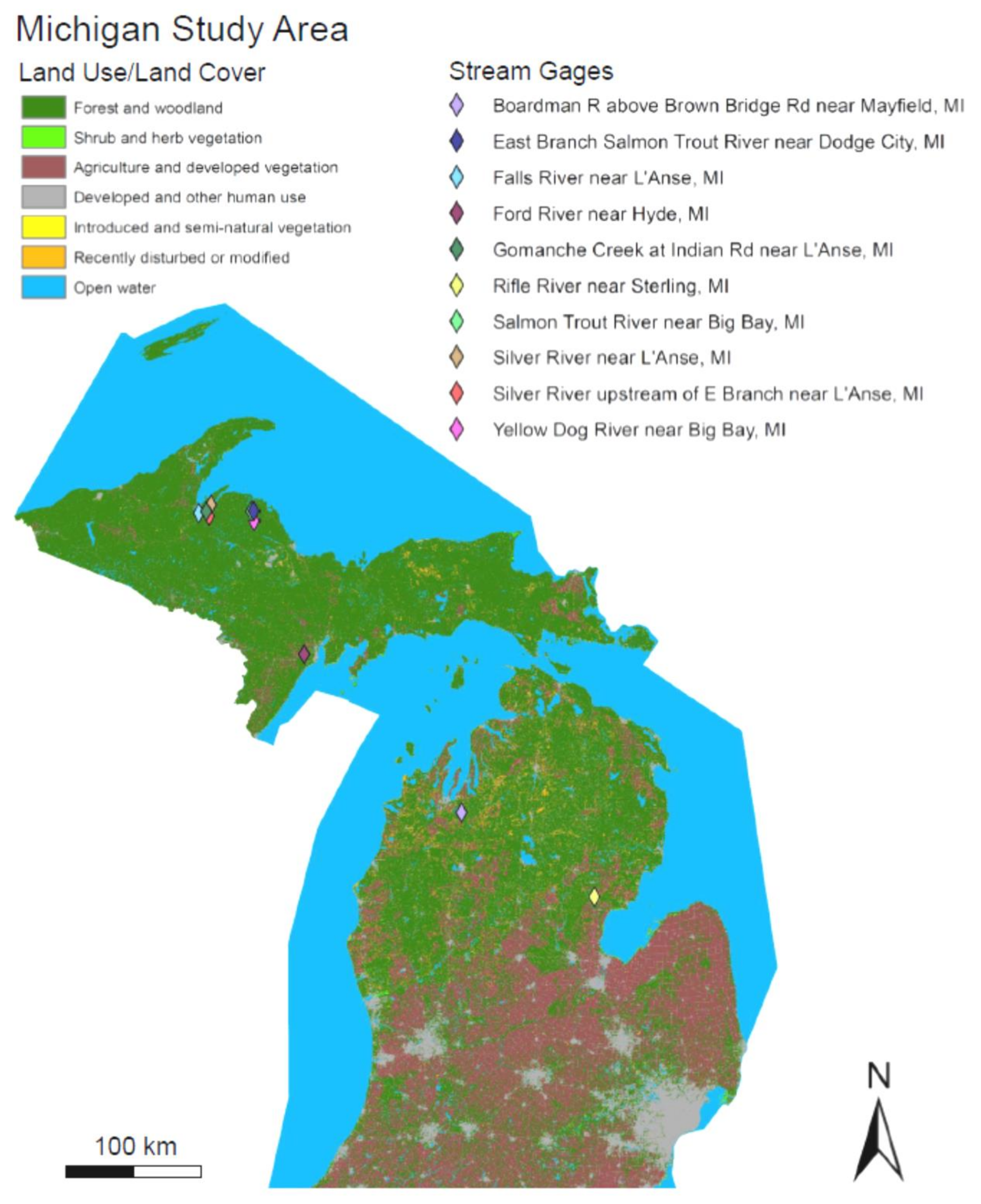
The state of Michigan is located in the Great Lakes region of the northern United States (Figure 1). Approximately 58% of the state consists of forest and woodland. Agriculture and developed urban land cover are primarily concentrated in the state’s more populated Lower Peninsula. Much of the surficial geology of Michigan is a result of Late Wisconsin glaciation, resulting in generally low relief topography and a nearly ubiquitous surficial layer of outwash, till, and lacustrine and/or moraine deposits [40].

This study was conducted on watersheds and gaging stations (

Table 1. Site locations and data records.

USGS Gage ID	Lat.	Long.	Streamflow Record	Stream SC Record	Missing Data Streamflow (%)	Missing Data SC (%)
Boardman R above Brown Bridge Road near Mayfield	44°39’24”	85°26’12”	1997-09-10–current	1997-11-05–1998-09-30	0	9.09
Falls River near L’Anse	46°44’05”	88°26’35”	2014-07-01–current	2014-09-30–2020-03-03	0	14.5
Ford River near Hyde	45°45’18”	87°12’07”	1954-10-01–current	1975-09-24–current	0	29.8 a
Gomanche Creek at Indian Road near L’Anse	46°45’04”	88°21’42”	2007-10-01–2013-09-29	2007-10-01–2013-09-29	0	35.9
Rifle River near Sterling	44°04’21”	84°01’12”	1937-01-13–current	1975-08-28–current	0	12.4 b
Salmon Trout River near Big Bay	46°46’56”	87°52’39”	2004-12-01–current	2004-12-01–2020-07-29	0	13.5 c
East Branch Salmon Trout River near Dodge City	46°47’09”	87°51’08”	2005-10-01–current	2005-12-06–current	0	1.95
Silver River near L’Anse	46°48’15”	88°19’01”	2001-10-01–current	2005-10-15–2013-09-29	0	35.2
Silver River Upstream of East Branch near L’Anse	46°43’16”	88°19’48”	2008-10-01–2013-09-29	2008-09-30–2013-09-29	0	35.2
Yellow Dog River near Big Bay	46°42’49”	87°50’26”	2004-12-01–2016-10-17	2004-12-22–2017-01-23	0	1.86

SC, specific conductance. ^a Calculation excludes no SC data period 1980-09-29 to 2011-04-25. ^b Calculation excludes no SC data period 1981-10-01 to 2011-06-07. ^c Calculation excludes no SC data period 2005-09-30 to 2013-06-28.

) selected from available U.S. Geological Survey (USGS) water data for the nation network [41]. Selection criteria were as follows: (1) availability of consecutive daily discharge and SC data for >1 year; (2) data spanning a time frame extending until >2010; (3) absence of major diversions or regulations through, e.g., dams, inflow from reservoirs, irrigation return flows or hydro electrical power plants; and (4) limited (i.e., <5%) urbanization or agriculture land use/land cover upstream of the stream gauge. For a reliable MK trend analysis, gages furthermore had to (5) exhibit a record of at least 50 years of daily streamflow records. All selected gages are unevenly distributed across the state, due mainly to flow regulation as well as urban/agricultural development in the state’s Lower Peninsula (Figure 1). Of the 10 gages that fit selection criteria 1 to 4, only two, Ford and Rifle River, fit selection criterion 5.

Daily discharge data of all considered gages reveal a seasonality related to precipitation and snowmelt trends, with peaks usually occurring between March and April and troughs in August through September. Daily SC data reveal an opposite pattern with the lowest values in spring, likely reflecting dilution from snowmelt, and the highest in summer/fall, consistent with more intense evapotranspiration and baseflow. There is a remarkable SC scatter among the different sites with mean values ranging from as low as 58.6 µS/cm at Yellow Dog River to as high as 420 µS/cm at Rifle River. This range in SC data could reflect the spatial variability of watershed bedrock and aquifer mineralogies. All Upper Peninsula rivers, with the exception of Ford River, drain Archean-age igneous and metamorphic rocks and associated sediments [42]. These lithologies consist primarily of low-solubility aluminosilicate minerals, which should produce low-SC stream- and groundwater [43,44]. By contrast, Ford, Boardman, and Rifle rivers drain larger proportions of more soluble carbonate/dolomite units of the Michigan Basin (e.g., Bayport Limestone, Niagara/Clinton Formations, etc.), which could explain the higher SC values of those streams. The overall SC variability attests to the importance of establishing temporally and spatially constrained and locally representative SC source end-members for a reliable hydrograph separation.

2.2. MOO Modeling of Baseflow

2.2.1. Conceptual Approach

This study estimates baseflow through optimization of the Lyne and Hollick (LH) RDF [45] (Equation (1)) via CMB benchmarks (Equation (2)) as follows:

$${\mathrm{q}}_{\mathrm{i}}={\mathrm{kq}}_{\mathrm{i}-1}+\frac{1+\mathrm{k}}{2}({\mathrm{y}}_{\mathrm{i}}-{\mathrm{y}}_{\mathrm{i}-1});{\mathrm{with}\mathrm{y}}_{\mathrm{i}}={\mathrm{b}}_{\mathrm{i}}+{\mathrm{q}}_{\mathrm{i}}$$

(1)

$${\mathrm{SC}}_{\mathrm{yi}}=\frac{{\mathrm{SC}}_{\mathrm{bi}}{\mathrm{b}}_{\mathrm{i}}+{\mathrm{SC}}_{\mathrm{qi}}{\mathrm{q}}_{\mathrm{i}}}{{\mathrm{y}}_{\mathrm{i}}}$$

(2)

where b_i, q_i, and y_i denote baseflow, quickflow (i.e., surface runoff), and total discharge on day i, respectively, and k is the RDF parameter. SC_bi and SC_qi are specific conductance values of the baseflow and quickflow sources on day i, and SC_yi represents the modeled stream SC value on day i. The approach is based on the assumption that when y_i = b_i, SC_bi = SC_yi and when y_i > b_i, SC_bi > SC_yi > SC_qi.

Two minimizing objective functions (F1, F2) are considered for the solution of Equations (1) and (2). The first gages the model’s performance of reproducing stream SC (SC_y) via the normalized Nash–Sutcliffe efficiency index (nNSE) [46] as follows:

$$\begin{gathered} \mathrm{F}1=1-\mathrm{nNSE}, \\ \mathrm{with}\mathrm{nNSE}=1-\frac{1}{{({\mathrm{n}}_{\mathrm{t}}+1)}^2}{\mathrm{and}\mathrm{n}}_{\mathrm{t}}=\frac{\mathrm{Standard}\mathrm{Deviation}}{\mathrm{RMSE}} \end{gathered}$$

(3)

The second objective function, F2, minimizes the occurrence of unrealistic events in which the measured river SC_y exceeds an interpolated baseflow SC_b end-member. To avoid optimization toward a local optimum (i.e., F2 = 0) by converging on a very low baseflow output (high k parameter) and short optimization period, F2 compares the sum of unrealistic SC_yi > SC_bi events to that of the more realistic SC_bi > SC_yi events as follows:

$$\mathrm{F}2={{\displaystyle \sum }}_{\mathrm{i}=1}^{\mathrm{n}}{({\mathrm{SC}}_{\mathrm{y}}>{\mathrm{SC}}_{\mathrm{b}})}_{\mathrm{i}}-{{\displaystyle \sum }}_{\mathrm{i}=1}^{\mathrm{n}}{({\mathrm{SC}}_{\mathrm{b}}>{\mathrm{SC}}_{\mathrm{y}})}_{\mathrm{i}}$$

(4)

Only optimization results for non-baseflow days (y_i > b_i, SC_yi ≠ SC_bi ≠ SC_qi) were considered. Periods of missing SC data (Table 1) were excluded, as were SC interpolation segments falling on a baseflow day coinciding with a missing SC record.

For the LH RDF in Equation (1), we followed the approach of [39] and (1) set the initial condition as y = q; (2) passed the LH RDF over the data up to three times (i.e., forward, backward, forward); (3) replaced the time step i −1 with i+1 when running the backward pass; (4) substituted y_i after the first pass by the computed baseflow calculated from the previous pass; (5) assigned baseflow to be equal to the current y_i if q_i is smaller than zero; and (6) applied ≥60 days flow prior to and at the end of the SC time series to resolve issues of “warm up” and “cool down” as the RDF is passed through the dataset [34].

The parameters k (Equation (1)) and SC_q (Equation (2)) are adjustable continuous variables determined via optimization. SC_b (Equation (2)) was generated via linear interpolation of SC_y records for consecutive baseflow days (i.e., y = b, q = 0) determined by the RDF in a given pass scenario in the optimization. This approach assumes that, when baseflow equals streamflow, the stream SC (SC_y) is representative for inflowing groundwater (SC_b). The interpolation of SC_y for all baseflow days is assumed to generate a baseflow SC_b time series that is representative for groundwater on baseflow days and when streamflow exceeds baseflow. Because of the baseflow and baseflow day timing dependency on k and RDF pass number, each iteration of k and pass number in the optimization translates into changing baseflow day occurrences, associated SC_b values, and period of daily SC_b interpolation. k optimization bounds were determined from trial runs for individual stream sites and were set from 0 (highest possible number of baseflow days) to an upper bound of >0.999 that was manually derived for each site to ensure >1 baseflow days.

To account for seasonality with potential differences in contributions from dilute snowmelt in spring vs. more saline surface runoff in summer/fall, SC_q was set as an adjustable parameter for three distinct seasonal time frames [47,48], i.e., November through February, March through June, and July through October. SC_q optimization bounds were set from a low of 0 µS/cm to an upper bound corresponding to the lower 25th percentile of the measured stream SC in the specific season. The selection of the lower 25th percentile over the absolute minimum reflects the influences of outliers, measurement error, as well as a priori uncertainty regarding the representativeness of the specific seasons for the studied river system.

2.2.2. MOO Algorithm

This study applied the Mixed Integer Distributed Ant Colony Optimization (MIDACO) algorithm [49] programmed in MATLAB. MIDACO is based on probability density functions that generate samples of iterates, referred to as ants or individuals [50,51] for the decision variables (in this study: k and SC_q) to be optimized. The ants cooperate on finding solutions to the problem through communication mediated by artificial pheromone trails. The seed operator introduces random changes into iterates, thereby, assisting in the search’s escape from local optima. Performance evaluations against other genetic algorithms such as Nondominated Sorting Genetic Algorithm (NSGA-II) [52,53] and Multi-Objective Particle Swarm Optimization (MOPSO) [54] indicate MIDACO to compare favorably [55,56]. This and the demonstrated performance on CPU time-expensive problems [57,58,59] support the utility of the algorithm for multiyear datasets as used in this study.

2.2.3. MOO Performance Evaluation

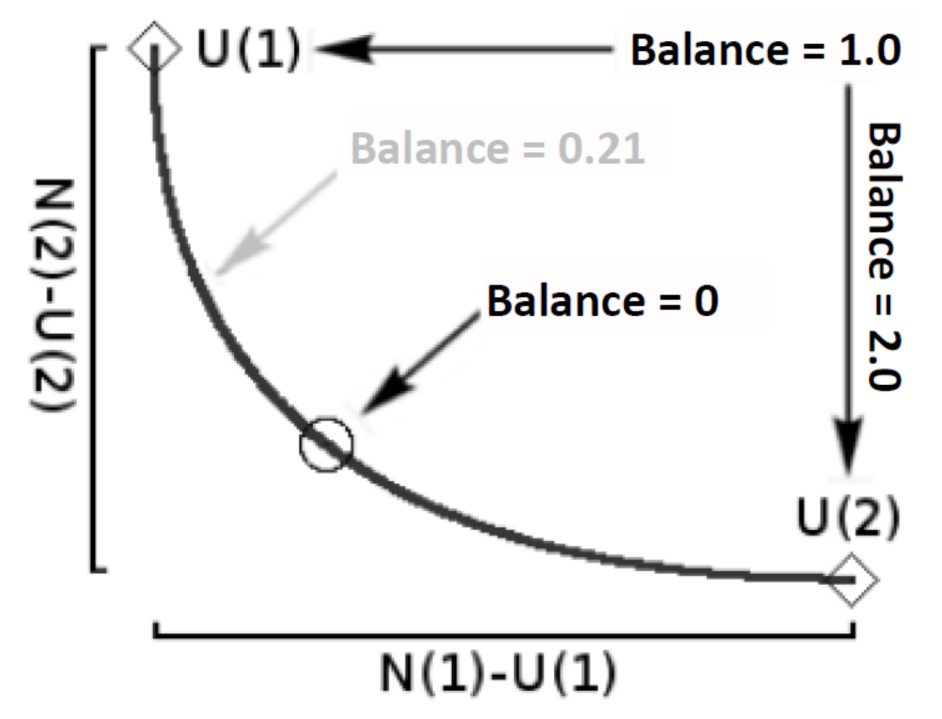
MOO generates not one unique solution, but a set of nondominated trade-off or compromise solutions (i.e., Pareto optimum solutions; see Figure 2 and Figure 3) from which one optimum can be selected [60,61,62]. MIDACO applies a Utopia–Nadir balance decomposition concept [59] to concentrate the search effort for the optimum trade-off solution on a particular segment of the Pareto front (Figure 2). The utopia (U) represents the global optimum (i.e., minimum) of the respective objective, while the nadir (N) corresponds to the worst possible (i.e., maximum) objective function. The search for a trade-off solution on the Pareto front is based on the average distance of a solution with respect to the U and N points of each objective. In MIDACO, the search is focused with the balance parameter (Figure 2). Set to zero, as done in this study, MIDACO will identify the trade-off solution on the central (or middle) part of the Pareto front to yield the best equally balanced solution among all objectives [49].

Another performance evaluation challenge relevant to this study is that there is no clear consensus on the optimum number of applied RDF passes. Running the RDF over multiple passes (forward, backward, forward, etc.) attenuates peaks and generates smoother baseflow hydrographs [63] and a lower total number of baseflow days [39], but this may come at a trade-off of missing short-term baseflow peaks typical for more flashy systems [11]. Based on previous baseflow analyses [11,39,64,65] that showed that both two-pass and three-pass implementations provide the best calibration results, we used outputs from both two-pass and three-pass model optimizations as a measure of uncertainty. All outputs were evaluated based on nNSE statistics (Equation (3)) of obtained trade-off solutions (

Table 2. MOO results for trade-off solutions.

Site and Model Scenario a	F1	F2	k (--)	SCq Nov–Feb (µS/cm)	SCq Mar–Jun (µS/cm)	SCq Jul–Oct (µS/cm)	Mean Baseflow (m3/s)	BFI (%) b
Boardman 2p	0.11	−120	0.96	248	159	242	3.16	91.6
Boardman 3p	0.10	−117	0.96	248	159	242	2.95	85.4
Falls 2p	0.14	−660	0.74	77	73	103	1.33	74.6
Falls 3p	0.14	−698	0.88	89	83	115	1.14	63.8
Ford 2p	0.17	−961	0.36	216	194	223	9.22	90.0
Ford 3p	0.19	−1169	0.56	246	219	259	8.19	79.9
Gomanche 2p	0.14	−545	0.41	104	84	113	0.09	84.1
Gomanche 3p	0.17	−545	0.10	111	98	126	0.10	86.4
Rifle 2p	0.16	−1576	0.25	247	235	327	8.68	90.6
Rifle 3p	0.18	−1653	0.27	309	280	354	8.34	87.1
Salmon Trout 2p	0.21	−448	0.50	69	43	58	0.16	91.8
Salmon Trout 3p	0.26	−411	0.66	69	53	63	0.15	87.7
East Branch Salmon Trout 2p	0.14	−1896	0.79	77	55	88	0.47	84.9
East Branch Salmon Trout 3p	0.14	−2067	0.99	85	62	91	0.39	69.1
Silver 2p	0.10	−816	0.72	66	46	76	1.49	74.3
Silver 3p	0.12	−898	0.71	76	55	84	1.35	67.3
Silver Upstream 2p	0.16	−519	0.27	20	25	29	0.61	84.6
Silver Upstream 3p	0.15	−482	0.90	32	41	50	0.37	51.2
Yellow Dog 2p	0.19	−1694	0.89	28	13	46	0.62	72.1
Yellow Dog 3p	0.21	−1620	0.83	33	17	47	0.61	70.6

^a 2p/3p indicates the use of either the two-pass or three-pass Lyne and Hollick recursive digital filter (RDF) in the MOO. ^b Baseflow index = mean baseflow to mean streamflow ratio.

).

2.3. Mann–Kendall Trend Analysis

2.3.1. Conventional MK Test

The nonparametric MK test was used to determine the statistical significance of time trends for modeled baseflow, streamflow, and BFIs for the Ford and Rifle rivers for a concurrent study period 12/01/1955–09/08/2020. As a first step in the test, datasets were reclassified into monthly, seasonal, and annual mean datasets to analyze short-term and long-term fluctuations (e.g., multiyear, decadal, and multidecadal events). The seasonal classification was based on the previously discussed three time frames of November through February, March through June, and July through October. Annual data refer to water years, which represent the 12-month period from October 1 through September 30, designated by the calendar year in which it ends.

After reclassification, the S statistic was calculated to predict an upward or downward trend of identically and independently distributed data as follows [66]:

$${\mathrm{S}}_{\mathrm{t}}={\displaystyle \sum }_{\mathrm{c}=1}^{\mathrm{n}-1}{\displaystyle \sum }_{\mathrm{d}=\mathrm{c}+1}^{\mathrm{n}}\mathrm{sign}\left({\mathrm{X}}_{\mathrm{d}}-{\mathrm{X}}_{\mathrm{c}}\right)$$

(5)

where X_c and X_d correspond the ranked values of the data, n is the length of the data record and

$$\mathrm{sign}\left({\mathrm{X}}_{\mathrm{d}}-{\mathrm{X}}_{\mathrm{c}}\right)=\left\{\begin{array}{c}1 \mathrm{when} {\mathrm{X}}_{\mathrm{d}}>{\mathrm{X}}_{\mathrm{c}} \\ 0 \mathrm{when} {\mathrm{X}}_{\mathrm{d}}={\mathrm{X}}_{\mathrm{c}}\\ -1 \mathrm{when} {\mathrm{X}}_{\mathrm{d}}<{\mathrm{X}}_{\mathrm{c}}\end{array}\right.$$

(6)

Next, the variance of S (σ²) was calculated assuming identically distributed data with a zero mean [67]:

$${\mathsf{\sigma }}^2=\left\{\mathrm{n}\left(\mathrm{n}-1\right)\left(2\mathrm{n}+5\right)-\left.{\displaystyle \sum }_{\mathrm{c}=1}^{\mathrm{n}}{\mathrm{t}}_{\mathrm{c}}\left(\mathrm{c}\right)\left(\mathrm{c}-1\right)\left(2\mathrm{c}+5\right)\right\}/18\right.$$

(7)

where t_c is the sum of t, which is the number of tied values to the extent of c [47]. Finally, the standardized MK statistic, Z (Equation (8)), was computed as a measure of significance of the trend [68]:

$$\mathrm{Z}=\left\{\begin{array}{c}\frac{{\mathrm{S}}_{\mathrm{t}}-1}{\sqrt{{\mathsf{\sigma }}^2}} \mathrm{if} {\mathrm{S}}_{\mathrm{t}}>0\\ 0 \mathrm{if} {\mathrm{S}}_{\mathrm{t}}=0\\ \frac{{\mathrm{S}}_{\mathrm{t}}+1}{\sqrt{{\mathsf{\sigma }}^2}} \mathrm{if} {\mathrm{S}}_{\mathrm{t}}<0\end{array}\right.$$

(8)

If |Z| > Zα/2, where α represents the chosen significance level (in this study: 5% with Z_0.025 = 1.96), then the null hypothesis is invalid, implying that the trend is significant and either positive (positive Z) or negative (negative Z).

2.3.2. Modified MK Test

Although the traditional MK test is appropriate for time series that are independent and identically distributed, autocorrelation (i.e., the persistence of previous observations) can cause an inflation of p-values resulting in increased type I errors; that is, accepting a trend as significant when, in fact, no trend exists [5]. The effect of long-term autocorrelation [69] was not considered a major concern for this study (<65 years of streamflow). However, short-term autocorrelation (STA) is of potential concern in trend analysis of monthly, seasonal, and annual mean hydrologic data [70]. In this study, we screened data for STA using the Ljung–Box test [71] from the R stats package. Following the approach of [5], we considered STA statistically significant for p-values ≤ 0.1 for lags ≤ 3 in the time series.

STA was accounted for in a modified MK analyses using six correction measures as implemented in the modifiedmk R package [72], specifically: pre-whitening (pw), bias-corrected pre-whitening (bcpw), trend-free pre-whitening (tfpw), variance correction after Hamed and Rao [73], variance correction after Yue and Wang [74] (hereafter referred to as vcHR98 and vcYH04, respectively), and block bootstrapping (bbs). Detailed descriptions on individual correction measures are provided elsewhere [73,75,76,77,78,79]; but briefly summarized, the pw, tfpw, and bcpw approaches are all based on the assumption that the time series of hydrological variables can be adequately described by an autoregressive process of order one, i.e., AR(1). In tfpw, a linear trend component is removed from the original data prior to pre-whitening [79], while in bcpw, ordinary least squares are used to bias-correct the lag-1 serial correlation coefficient [80]. The vc approach detrends data using Sen’s slope and the lag-1 autocorrelation coefficient of the ranks of the data. It calculates effective sample size using the ranks of significant serial correlation coefficients, which are used to correct the inflated (or deflated) variance of the test statistic. The vcHR98 method uses only significant lags of autocorrelation coefficients in calculating the effective sample size, whereas the vcYH04 approach uses correlation coefficients for all lags [72]. In bbs, predetermined block lengths are used in resampling the original time series, thus retaining the memory structure of the data. The test statistic is then calculated for each sample, and its probability distribution is estimated. Because any existing trend will be eliminated due to shuffling, the derived distribution is that of the test statistic for trend-free data [78]. Assuming a confidence interval of 95% and a sampling size of 2000 [81], the hypothesis of no trend is rejected if the trend of the original data series is outside the 5% and 95% percentiles of the ranked trends of the resamples. Block lengths are automatically selected in modifiedmk using the number of contiguous significant serial correlations and a default eta (η) parameter of 1 as per [77]. Results of all MK tests are listed in Supplementary Table S1.

3. Results and Discussion

3.1. Baseflow Results

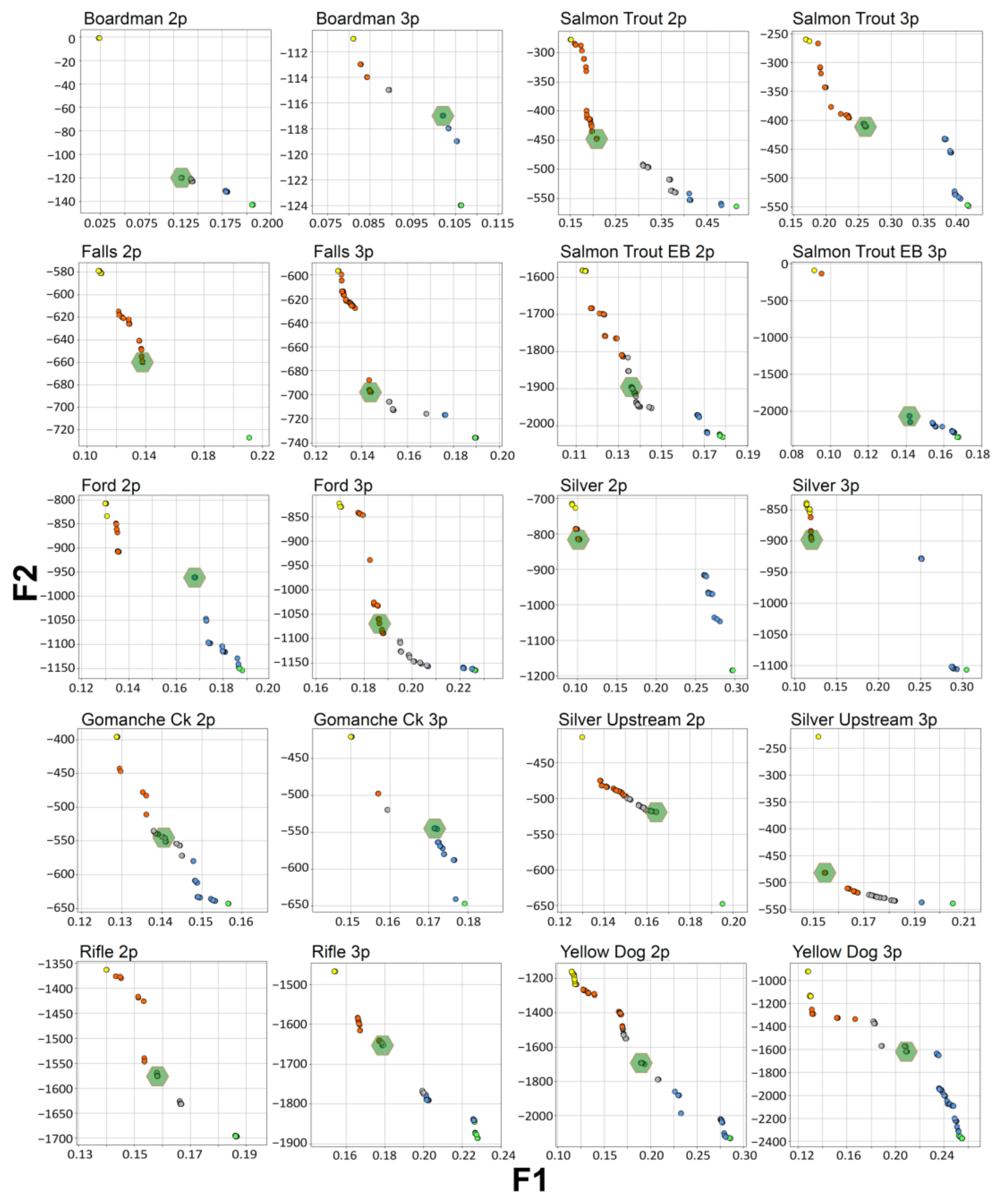
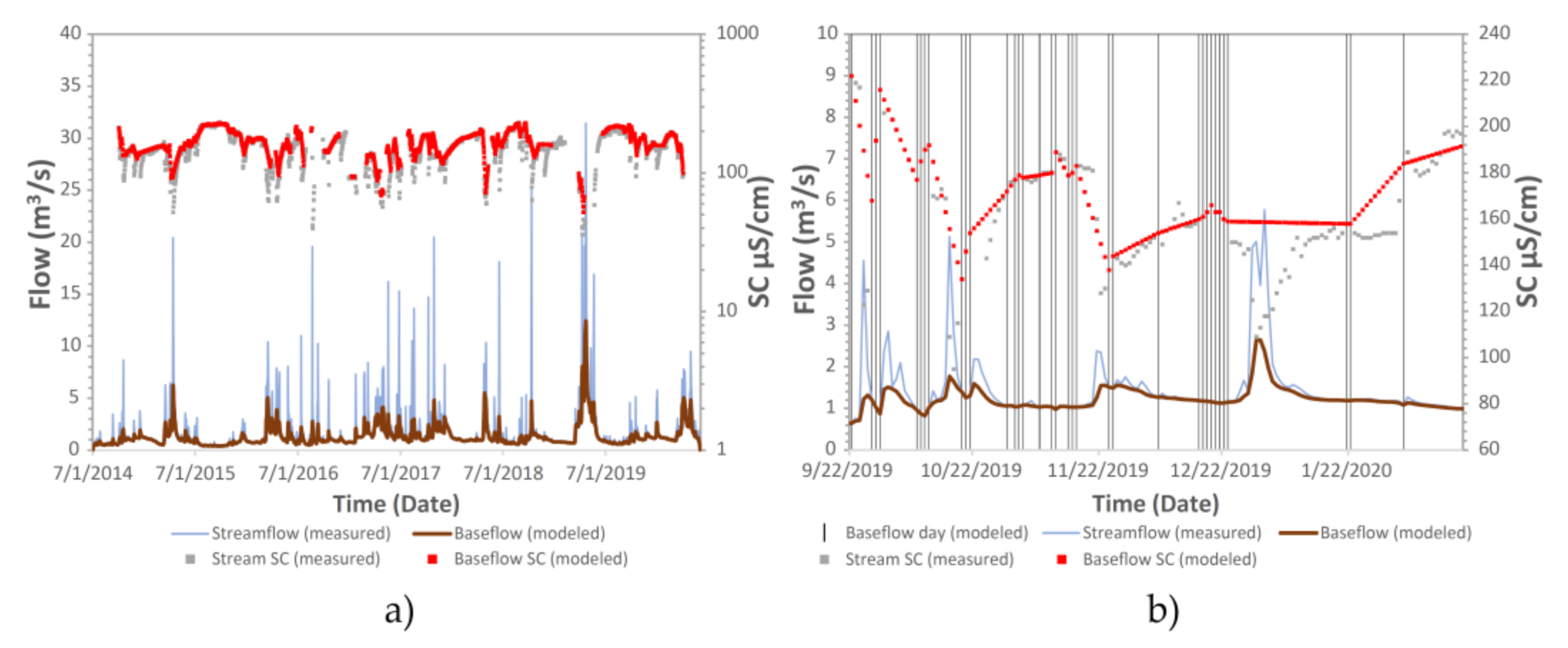
The results of the MOO models are shown in Figure 3 and Table 2. Pareto optimum fronts for all 10 USGS gages clearly highlight the opposing nature of the objective functions, as an optimized F1 (Equation (3)) is accomplished by an increased error in F2 (Equation (4)) and vice versa. Pareto optimum fronts furthermore exhibited nonconvex, as well as disconnected segments (Figure 3), which is consistent with the nonlinear nature of the optimization problem [62]. All trade-off solutions reveal a seasonality in the calibrated SC_q that follows the expected pattern of more saline composition in the dry period July through October and more dilute SC_q in the snowmelt period March through June (Table 2). Importantly, all calibrated SC_q values were well below the optimization bounds, i.e., the lower 25th of the seasonal SC_y. These observations and the good to very good nNSE (i.e., 1−F1) statistics [46] of the trade-off solutions indicate that the applied modeling approach describes the watersheds well (see, e.g., Figure 4a).

The two-pass scenario generally yields superior results for objective function 1 but is outperformed by the three-pass scenario for objective function 2. This can be explained by the attenuating effect of an RDF pass number increase from 2 to 3 on the baseflow hydrograph that results in (1) lower occurrences of baseflow days, (2) less pronounced baseflow responses to short-term discharge peaks, and (3) lower overall occurrences of SC_y exceeding SC_b. This is accomplished at the trade-off of potentially missing several short-term or “flashy” baseflow SC_b dilution events required for a better objective function 1 calibration. On the other hand, short-term SC_b dilutions are well reproduced by the two-pass scenario at the cost of not representing many of those as dilute quick flow peaks, and thus not capturing all SC_y peaks underneath the SC_b interpolation line (Figure 4b). There is a tendency for the MOO to counteract the attenuating effect on baseflow amounts from increasing the LH RDF pass number from 2 to 3 by decreasing the k parameter. This pattern is one of the key advantages of the applied method over traditional baseflow quantification measures, as it limits the uncertainty in the baseflow and BFI outputs to relatively narrow ranges (e.g., BFI = 70.6–72.1% at Yellow Dog River).

Mean baseflow estimates obtained from both the two-pass and three-pass MOO scenarios vary between 0.09 ± 0.001 m³/s at Gomanche Creek and 8.70 ± 0.51 m³/s at Ford River. BFIs range from 67.9% ± 16.7% at the Silver River upstream to 89.7% ± 2.04% at Salmon Trout River. Seasonal patterns of baseflow are similar for all gages, with the lowest values in the annual dry period of late summer/early fall (August–October) and the highest values in the spring snowmelt period (March–May) and in the fall/early winter (November–December). The latter distinct “fall bump” in baseflow (Figure 5) that follows snowmelt recession is attributed to a reversal in the hydraulic gradient as stream levels and rates of evapotranspiration drop [33,82]. The lag between the annual streamflow and mean baseflow maxima is relatively short, ranging from 0 days at Falls River, Gomanche Creek, and Rifle River to up to 10 days at Salmon Trout River East Branch.

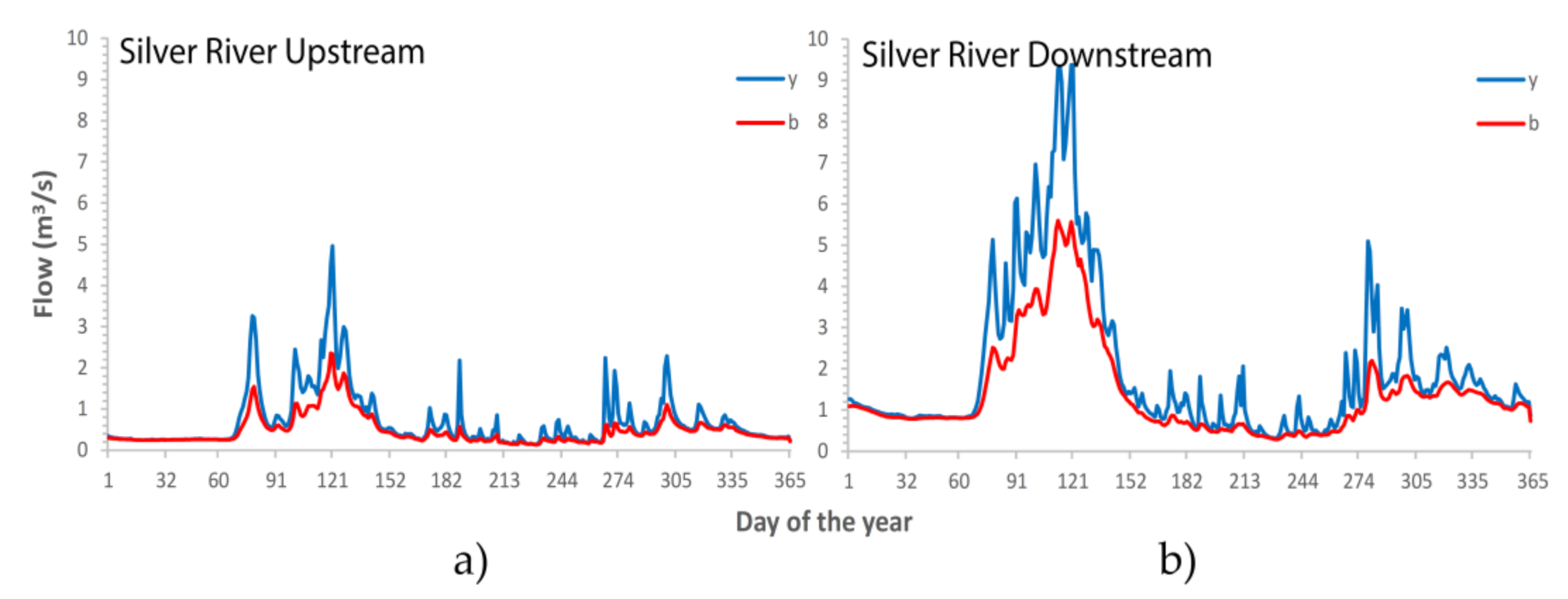
Using concurrent data for the Silver River watershed, for which data from two stream gages were analyzed, mean baseflow increases downstream from 0.49 to 1.38 m³/s while the mean BFI decreases downstream from 0.68 to 0.70. This spatial pattern is consistent with hydraulic loading toward the lowlands, which increases baseflow volume but not the BFI due to the cumulative effects of tributary inflow. Additionally, the thicker unsaturated zone at the higher-altitude upstream site should result in less pronounced head reversals and, thus, a lower “fall bump” in baseflow (Figure 5a,b).

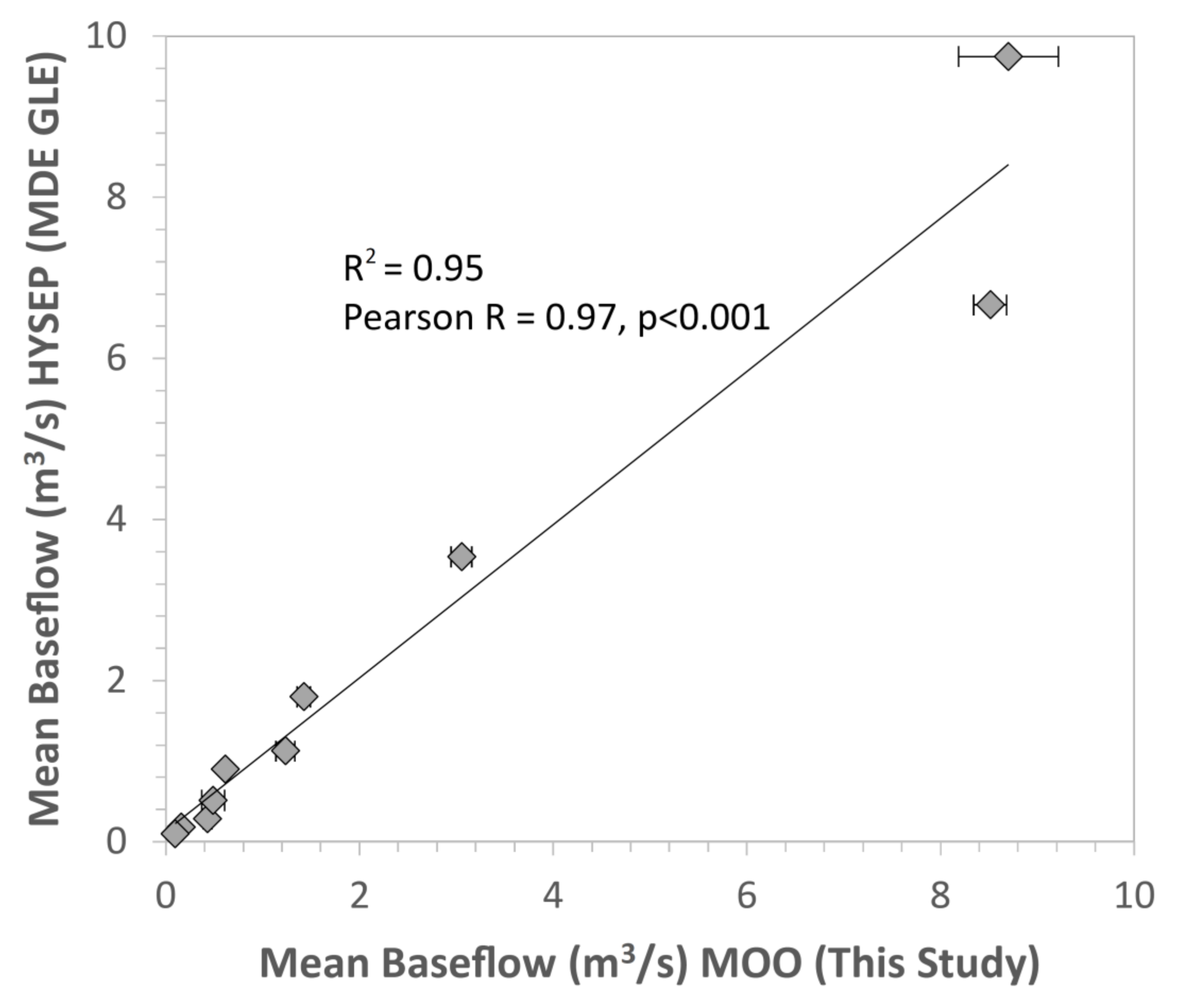
There is a strong positive correlation (Pearson R = 0.97, p < 0.001) between our MOO-derived baseflow estimates and previous estimates [83] derived upon the more standardized HYSEP program [27] which applies simple graphical methods for baseflow quantification (Figure 6). It is, however, not clear to what degree deviations from the regression line in Figure 6 should be attributed to methodological differences or comparison of streams with data from different time periods. To the authors’ knowledge, there is no clear information about the specific dataset length of the HYSEP-based estimates. We, however, have found striking temporal patterns in our estimates that could very well explain the deviations from the trendline. As an illustration, for the two streams for which long-term data are available—Ford and Rifle rivers—there is a near 30-year SC data gap from 1980/1981 until 2011 (Table 1). Mean baseflow estimates for the Ford and Rifle rivers change from 7.82–7.88 m³/s, respectively, if the concurrent streamflow and SC_y dataset of 1975–1981 is used, to values of 9.29–9.94 m³/s, respectively, if the concurrent dataset of 2011–2020 is used. This and the remarkable variability in streamflow and SC values of the sites considered highlight the dynamic characteristics of this setting and the associated challenge of reliable hydrologic trend analysis in this area.

3.2. Autocorrelation Results

For both long-term monitoring sites, significant STA is documented, particularly in the higher-frequency (monthly/seasonal) baseflow and streamflow time series (

Table 3. Ljung–Box (L-B) test results for 1956–2019 time series.

USGS Site	Data	Time Series	L-B Test Statistic lag 1	p-Value Lag 1	L-B Test Statistic Lag 2	p-Value Lag 2	L-B Test Statistic Lag 3	p-Value Lag 3	STA b
FORD RIVER NEAR HYDE, MI	Streamflow	Monthly	104	<0.1	105	<0.1	136	<0.1	yes
		Seasonal	8.60	<0.1	17.2	<0.1	105	<0.1	yes
		Annual	2.15	0.14	2.84	0.24	3.20	0.36	no
	Baseflow	Monthly	109	<0.1	110	<0.1	139	<0.1	yes
		Seasonal	7.56	<0.1	16.1	<0.1	102	<0.1	yes
		Annual	1.99	0.16	2.64	0.27	3.05	0.38	no
	BFI a	Monthly	48.0	<0.1	49.7	<0.1	54.4	<0.1	yes
		Seasonal	9.49	<0.1	24.1	<0.1	72.8	<0.1	yes
		Annual	0.86	0.35	2.64	0.27	3.30	0.35	no
RIFLE RIVER NEAR STERLING, MI	Streamflow	Monthly	168	<0.1	177	<0.1	185	<0.1	yes
		Seasonal	7.28	<0.1	17.9	<0.1	101	<0.1	yes
		Annual	3.63	<0.1	4.84	<0.1	5.15	0.16	no
	Baseflow	Monthly	193	<0.1	206	<0.1	213	<0.1	yes
		Seasonal	7.51	<0.1	18.6	<0.1	105	<0.1	yes
		Annual	3.44	<0.1	4.41	0.11	4.80	0.19	no
	BFI a	Monthly	24.5	<0.1	24.9	<0.1	27.2	<0.1	yes
		Seasonal	1.45	0.23	5.96	<0.1	52.8	<0.1	no
		Annual	4.04	<0.1	8.85	<0.1	10.0	<0.1	yes

^a Baseflow index = mean baseflow to mean streamflow ratio. ^b STA = short-term autocorrelation based on the highest p-value of lag 1–3 analyses.

). As typically seen in hydrologic data [70], STA is positive (Ljung–Box statistics > 0) for all timeseries, in that, high values are followed by high values and low values are followed by low values. Interestingly, STA is most significant in baseflow, followed by streamflow and BFI (Table 3). This observation is consistent with the stronger memory effect of slower moving groundwater and baseflow as compared to streamflow (and BFI) that are more influenced by sudden, quickflow responses to short-term rain events [84]. Comparing results for a concurrent time period from both sites, STA is slightly more pronounced at Rifle River (mean lag 1 to lag 3 Ljung–Box test statistic: 58.7, p = 0.04) than at Ford River (mean lag 1 to lag 3 Ljung–Box test statistic: 45.9, p = 0.09). This observation is consistent with the higher overall BFI value for the Rifle River (Table 2).

The presence of STA generally mandates large sampling sizes (i.e., multidecade monitoring durations) for hydrologic trend analysis [70]. However, the lower degree of STA in the BFI time series (Table 3) indicates that the BFI parameter may be a useful alternative over streamflow or baseflow data for trend analyses over shorter time frames.

3.3. MK Test Results

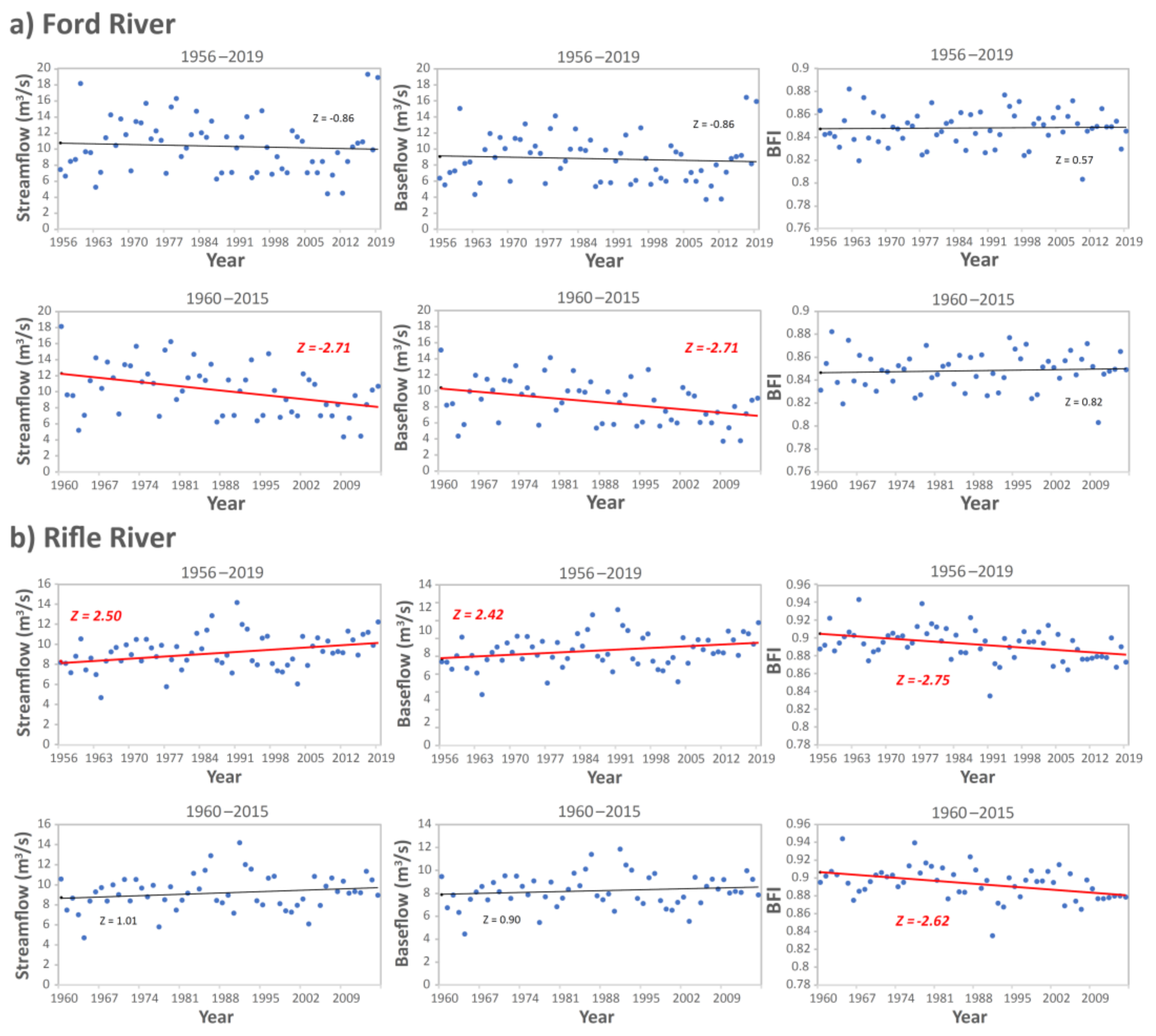
Despite the concurrent data, proximity of the monitoring stations (~313 km), and the largely undisturbed nature of both watersheds, MK trend analysis reveals strikingly contrasting results for Ford and Rifle rivers (Supplementary Table S1 and Figure 7). For Ford River, all analyses yielded no significant trend, with the exception of annual BFI analyzed via the vcYH04 method (Z value = 2.09). For Rifle River, nearly all MK tests revealed statistically significant trends, i.e., positive for streamflow and baseflow (Z value = 1.74 to 15.9; mean value = 3.67) and negative for BFI (Z value = −1.94 to −14.7; mean value = −4.26). Trends were most significant in the monthly and least significant in the annual time series. Among the different methods applied for Rifle River, the vcHY04 method produced the most significant results while the pw method produced the least significant Z values.

Even though numerous studies have tested appropriate MK approaches for addressing potential effects of STA, these approaches are not universally accepted, and studies have applied multiple correction methods as a measure for uncertainty [68,85]. We have no preference for any of the applied correction methods and, thus, rely on the results of all procedures as a measure for uncertainty. Nevertheless, the annual BFI trend at Ford River from the vcYH04 method is considered a Type I error because (1) it was the only statistically significant result and (2) the variance correction approach has shown to be particularly prone to such errors at small sampling sizes, i.e., annual data as compared to seasonal or monthly time series [78]. We, therefore, conclude no significant climate change effects on streamflow and groundwater recharge in the Upper Peninsula Ford River watershed. In the Lower Peninsula Rifle watershed, increases in baseflow (and by implication, groundwater recharge) are observed, albeit at a lower rate than the surface runoff component (decreasing BFI). The more attenuated increase in baseflow suggest groundwater recharge to be less impacted by climatic drivers than surface runoff components; the latter likely contributing to the reported flood frequency increases in the region [2,10].

To further evaluate the potential causes for the trends (and lack thereof), results were compared to previously reported trend analyses for climatic parameters in the region, i.e., 1960−2015 total precipitation (P), minimum temperature (T_min), and maximum temperature (T_max) [5], as well as 1960−2009 total snowfall (SF) and snow depth (SD) [86]. For these climatic parameters, there were also strikingly different results between Michigan’s Upper and Lower Peninsula. The former exhibited a significant decline in P coupled with significant upward trends in T_min and SF and no significant trends in T_max and SD. The reported trends are generally indicative for evapotranspiration rate (ET) increase [87], extended growing season length [88], a transition from rain to snow precipitation [86], larger accumulation of spring snowmelt pulses [3] and shifts in snowmelt-related streamflow timing to earlier dates [85]. These patterns have apparently not caused any significant baseflow or BFI trends; however, despite the concurrent decrease in P, which should exacerbate streamflow and baseflow declines caused by more intense ET. As will be discussed at more detail later, the lack of Ford River stream- and baseflow trends is likely associated with the high-water-flow years 1960, 2017, and 2019 (see Figure 7a, left and middle panels), which were not accounted for in the P, T_min, T_max, SF, and SD trend analyses.

In the Lower Peninsula, P and T_min increased, SD decreased, and no significant trends were reported for T_max or SF. In contrast to the Northern Peninsula, these findings are generally more indicative for a snow- to rain transition [86], as well as a lower accumulation of snowpack storage and a lower snowmelt pulse [3]. In the Rifle River watershed, these patterns apparently led to increases in baseflow and streamflow; the latter increasing at a higher rate, as evidenced by the decreasing BFI. A compounding factor on these trends in the Rifle watershed could be the documented increasing frequency and intensity of heavy rain events, which reportedly have contributed to more frequent flooding [2] and apparently favor the surface runoff over the baseflow component. Interestingly, the significant upward trend in T_min, and by association ET, in the Lower Peninsula also does not appear to exert significant effects, as it is insufficient to offset the upward trend in P. Time series major ion and stable isotope data may provide further insights as to the specific effects of ET changes on the stream hydrograph [89,90,91].

3.4. Transferability of Results

It is important to note that the previously published P, SF, SD, T_min, and T_max trends we used for the comparison with baseflow and BFI trends were derived upon slightly shorter study periods and should, as such, be treated with caution for longer-term implications. The importance of this limitation is well exemplified when comparing our annual mean streamflow MK test results to those previously reported (Figure 7). For their study period 1960−2015, [5] discerned a statistically significant downward trend in streamflow for Ford River and an insignificant upward trend in streamflow for Rifle River. We were able to reproduce these results through the traditional and modified MK tests for this particular time frame. However, extending the time period to include the years 1956, 1957, 1958, 1959, 2016, 2017, and 2018 completely changes these results (Figure 7), with Ford River streamflow trends becoming insignificant and Rifle River trends becoming significant, even if STA is accounted for (as shown by the block bootstrapped Z values shown in Figure 7). This change in MK trend test results for the Ford River is likely associated with the fact that both tails of the 1956−2019 time period, specifically the water years 1960, 2017, and 2019, coincide with the highest flow water years of the study period. While a change in the study period from 1960−2015 to 1956−2019 alters calculated annual streamflow and baseflow trends for both rivers, there is no change in the BFI trend in that it remains insignificant for Ford River and significant (i.e., negative) for Rifle River (Figure 7). This persistence again highlights the value of the BFI parameter, if objectively constrained, for a refined hydrological trend analysis for watersheds where streamflow or baseflow statistics indicate no significant trend.

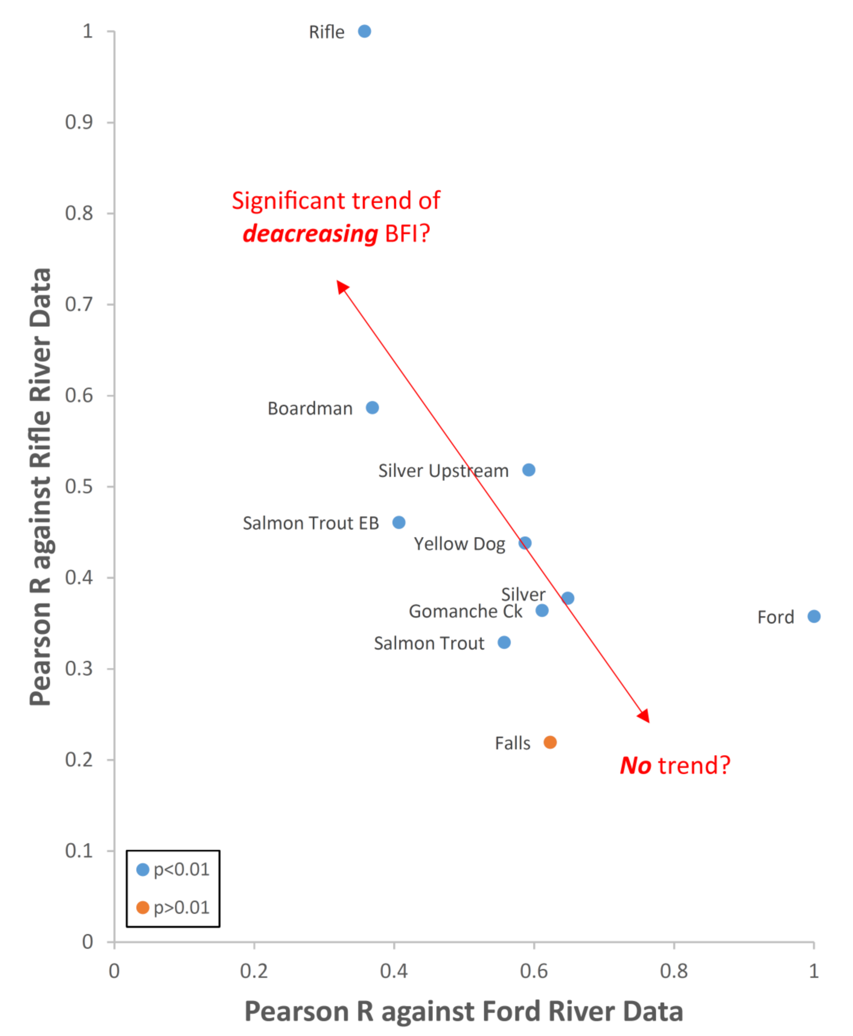
As a first step to discern potential long-term BFI trends across the study area, i.e., in the remaining eight stream sites that meet selection criteria 1 through 4 (see Section 2.1), a linear regression analysis was conducted against concurrent monthly BFI data from the long-term record stream sites, Ford and Rifle Rivers (Figure 8). The results show a strong effect of spatial autocorrelation, in that, stream gages closest to the long-term sites show stronger positive correlation coefficients for monthly BFI and vice versa. This suggests that the MK test results for Ford River (no trend in BFI) could also apply to the other sites located in the Upper Peninsula, while Rifle River MK test results (negative BFI) are potentially also valid for Boardman River; the sole other gage considered from the Lower Peninsula. Interestingly, of all sites considered, only the Silver River Upstream gage exhibited a strong and significant (Pearson R > 0.5, p-value <0.01) correlation with data from both Ford and Rifle rivers. This suggests somewhat of an intermediate BFI pattern in Silver River in relation to the long-term monitoring sites and should be investigated further. Conversely, the Salmon Trout East Branch site shows only a moderate (Pearson R < 0.5; p < 0.01) correlation for both sites, which indicates a more localized response to temperature and precipitation change. However, because this correlation analysis relies on concurrent BFI data covering different time spans, a comparison of correlation statistics between different sites should be treated with some caution [92]. Moreover, despite the variability of recession properties across the study catchments, recent work has shown that streamflow (and potentially also BFI) spatial correlation among neighboring watersheds can be overwhelmed by the spatial variability of frequency and intensity of effective rainfall events [93]. A detailed analysis of watershed-specific trends in P, SF, SD, T_min, and T_max and a comparison with associated BFI patterns may provide more valuable predictors for trends in ungaged watersheds.

4. Conclusions and Implications

This study highlights the value of MOO for objective baseflow modeling and long-term hydrologic trend analysis in lowland streams. One key advantage of the hydrograph separation method presented in this paper is that it accounts for difficult-to-measure spatial and temporal variations in baseflow and quickflow chemistry (i.e., SC). Our study specifically emphasizes the importance of site-specific determinations of MOO parameters k, SC_q, and SC_b rather than the application of non-distributed parameters for one region. As such, our results should be treated as cursory estimates of baseflow trends in undisturbed parts of the state that should be refined and validated not only with new daily flow and SC geochemical data for MOO, but also with estimates from other, independent baseflow quantification approaches [94].

The MK trend analysis reveals an important finding, i.e., decreasing P, increasing T_min, and a shift in P from rain- to snowfall in the state’s Upper Peninsula exerted no significant effects on baseflow or BFI, while increasing P, T_min, and a transition from snow- to rainfall in the Lower Peninsula have increased baseflow and decreased the BFI. The latter observation suggests an attenuated effect on groundwater recharge that should be considered carefully in future groundwater availability projections. Unlike the streamflow and baseflow parameters, the trend for BFI is persistent for both a shorter-term (1960−2015) and longer-term (1956−2019) dataset. This finding in conjunction with the lower degree of STA effects supports the value of the BFI parameter in trend analysis over shorter (i.e., <50 year) time frames.

Future research should address extrapolation of our baseflow and BFI values to ungaged watersheds for more refined regional assessments of climate-change-induced trends. Studies should furthermore test the utility of the presented MOO approach to calibrate and validate soil water balance models in complex watersheds with pronounced spatiotemporal variability in the stream hydrograph and SC.

References

- U.S. Global Change Research Program. Fourth National Climate Assessment Chapter 21: Midwest. Available online: https://nca2018.globalchange.gov/chapter/21 (accessed on 22 September 2020).
- Wuebbles, D.; Cardinale, B.; Cherkauer, K.; Davidson-Arnott, R.; Hellmann, J.; Infante, D.; Johnson, L.; de Loë, R.; Lofgren, B.; Packman, A.; et al. An Assessment of the Impacts of Climate Change on the Great Lakes by Scientists and Experts from Universities and Institutions in the Great Lakes Region; Environmental Law & Policy Center: Chicago, IL, USA, 2019; p. 74. [Google Scholar]
- Christiansen, D.E.; Walker, J.F.; Hunt, R.J. Basin-Scale Simulation of Current and Potential Climate Changed Hydrologic Conditions in the Lake Michigan Basin, United States; Scientific Investigations Report; U.S. Geological Survey: Reston VA, USA, 2014; p. 86. [Google Scholar]
- Markstrom, S.L.; Hay, L.E.; Ward-Garrison, D.C.; Risley, J.C.; Battaglin, W.A.; Bjerklie, D.M.; Chase, K.J.; Christiansen, D.E.; Dudley, R.W.; Hunt, R.J.; et al. Integrated Watershed-Scale Response to Climate Change for Selected Basins across the United States; Scientific Investigations Report; U.S. Geological Survey: Reston, VA, USA, 2012; p. 153. [Google Scholar]
- Norton, P.A.; Driscoll, D.G.; Carter, J.M. Climate, Streamflow, and Lake-Level Trends in the Great Lakes Basin of the United States and Canada, Water Years 1960–2015; Scientific Investigations Report; U.S. Geological Survey: Reston, VA, USA, 2019; p. 58. [Google Scholar]
- Gebert, W.A.; Walker, J.F.; Kennedy, J.L. Estimating 1970-99 Average Annual Groundwater Recharge in Wisconsin Using Streamflow Data; Open-File Report; U.S. Geological Survey: Reston, VA, USA, 2011. [Google Scholar]
- Neff, B.P.; Day, S.M.; Piggott, A.R.; Fuller, L.M. Base Flow in the Great Lakes Basin; Scientific Investigations Report; U.S. Geological Suvey: Reston, VA, USA, 2005. [Google Scholar]
- Hodgkins, G.A.; Dudley, R.W.; Aichele, S.S. Historical Changes in Precipitation and Streamflow in the U.S. Great Lakes Basin, 1915–2004; Scientific Investigations Report; Geological Survey (U.S.): Reston, VA, USA, 2007. [Google Scholar]
- Croley, T.; Luukkonen, C. Potential Effects of Climate Change on Ground Water in Lansing, Michigan. JAWRA J. Am. Water Resour. Assoc. 2007, 39, 149–163. [Google Scholar] [CrossRef]
- Gronewold, A.D.; Rood, R.B. Recent Water Level Changes across Earth’s Largest Lake System and Implications for Future Variability. J. Gt. Lakes Res. 2019, 45, 1–3. [Google Scholar] [CrossRef]
- Zhang, J.; Zhang, Y.; Song, J.; Cheng, L. Evaluating Relative Merits of Four Baseflow Separation Methods in Eastern Australia. J. Hydrol. 2017, 549, 252–263. [Google Scholar] [CrossRef]
- Shao, G.; Zhang, D.; Guan, Y.; Sadat, M.A.; Huang, F. Application of Different Separation Methods to Investigate the Baseflow Characteristics of a Semi-Arid Sandy Area, Northwestern China. Water 2020, 12, 434. [Google Scholar] [CrossRef] [Green Version]
- Zhang, Y.; Ahiablame, L.; Engel, B.; Liu, J. Regression Modeling of Baseflow and Baseflow Index for Michigan USA. Water 2013, 5, 1797–1815. [Google Scholar] [CrossRef] [Green Version]
- Ahiablame, L.; Chaubey, I.; Engel, B.; Cherkauer, K.; Merwade, V. Estimation of Annual Baseflow at Ungauged Sites in Indiana USA. J. Hydrol. 2013, 476, 13–27. [Google Scholar] [CrossRef]
- Beatty, S.J.; Morgan, D.L.; McAleer, F.J.; Ramsay, A.R. Groundwater Contribution to Baseflow Maintains Habitat Connectivity for Tandanus Bostocki (Teleostei: Plotosidae) in a South-Western Australian River. Ecol. Freshw. Fish 2010, 19, 595–608. [Google Scholar] [CrossRef]
- Boutt, D.F.; Hyndman, D.W.; Pijanowski, B.C.; Long, D.T. Identifying Potential Land Use-Derived Solute Sources to Stream Baseflow Using Ground Water Models and GIS. Groundwater 2001, 39, 24–34. [Google Scholar] [CrossRef]
- Choi, B.; Kang, H.; Lee, W.H. Baseflow Contribution to Streamflow and Aquatic Habitats Using Physical Habitat Simulations. Water 2018, 10, 1304. [Google Scholar] [CrossRef] [Green Version]
- McCallum, J.L.; Cook, P.G.; Brunner, P.; Berhane, D. Solute Dynamics during Bank Storage Flows and Implications for Chemical Base Flow Separation. Water Resour. Res. 2010, 46, W07541. [Google Scholar] [CrossRef] [Green Version]
- Murray, B.; Zeppel, M.; Hose, G.; Eamus, D. Groundwater-Dependent Ecosystems in Australia: It’s More than Just Water for Rivers. Ecol. Manag. Restor. 2008, 4, 110–113. [Google Scholar] [CrossRef]
- Power, G.; Brown, R.S.; Imhof, J.G. Groundwater and Fish—Insights from Northern North America. Hydrol. Process. 1999, 13, 401–422. [Google Scholar] [CrossRef]
- Reichard, J.S.; Brown, C.M. Detecting Groundwater Contamination of a River in Georgia, USA Using Baseflow Sampling. Hydrogeol. J. 2009, 17, 735–747. [Google Scholar] [CrossRef]
- Malcolm, I.A.; Soulsby, C.; Youngson, A.F.; Hannah, D.M.; McLaren, I.S.; Thorne, A. Hydrological Influences on Hyporheic Water Quality: Implications for Salmon Egg Survival. Hydrol. Process. 2004, 18, 1543–1560. [Google Scholar] [CrossRef]
- Combalicer, E.; Lee, S.-K.; Ahn, S.; Kim, D.; Im, S. Comparing Groundwater Recharge and Base Flow in the Bukmoongol Small-Forested Watershed, Korea. J. Earth Syst. Sci. 2008, 117, 553–566. [Google Scholar] [CrossRef] [Green Version]
- Arnold, J.G.; Muttiah, R.S.; Srinivasan, R.; Allen, P.M. Regional Estimation of Base Flow and Groundwater Recharge in the Upper Mississippi River Basin. J. Hydrol. 2000, 227, 21–40. [Google Scholar] [CrossRef]
- Nielsen, M.G.; Westenbroek, S.M. Groundwater Recharge Estimates for Maine Using a Soil-Water-Balance Model—25-Year Average, Range, and Uncertainty, 1999 to 2015; Scientific Investigations Report; U.S. Geological Survey: Reston, VA, USA, 2019; p. 68. [Google Scholar]
- Zomlot, Z.; Verbeiren, B.; Huysmans, M.; Batelaan, O. Spatial Distribution of Groundwater Recharge and Base Flow: Assessment of Controlling Factors. J. Hydrol. Reg. Stud. 2015, 4, 349–368. [Google Scholar] [CrossRef] [Green Version]
- Sloto, R.A.; Crouse, M.Y. HYSEP: A Computer Program for Streamflow Hydrograph Separation and Analysis: U.S. Geological Survey Water-Resources Investigations Report 96–4040; U.S. Geological Survey: Reston, VA, USA, 1996; p. 46. [Google Scholar]
- Aksoy, H.; Kurt, I.; Eris, E. Filtered Smoothed Minima Baseflow Separation Method. J. Hydrol. 2009, 372, 94–101. [Google Scholar] [CrossRef]
- Wahl, K.L.; Wahl, T.L. Determining the Flow of Comal Springs at New Braunfels, Texas; Texas Water ’95; American Society of Civil Engineers: San Antonio, TX, USA, 1995; pp. 77–86. [Google Scholar]
- Rammal, M.; Archambeau, P.; Erpicum, S.; Orban, P.; Brouyère, S.; Pirotton, M.; Dewals, B. Technical Note: An Operational Implementation of Recursive Digital Filter for Base Flow Separation. Water Resour. Res. 2018, 54, 8528–8540. [Google Scholar] [CrossRef]
- Rorabaugh, M.I. Estimating Changes in Bank Storage and Ground-Water Contribution to Streamflow. Int. Assoc. Sci. Hydrol. 1964, 63, 432–441. [Google Scholar]
- Cartwright, I.; Gilfedder, B.; Hofmann, H. Contrasts between Estimates of Baseflow Help Discern Multiple Sources of Water Contributing to Rivers. Hydrol. Earth Syst. Sci. 2014, 18, 15–30. [Google Scholar] [CrossRef] [Green Version]
- Miller, M.P.; Susong, D.D.; Shope, C.L.; Heilweil, V.M.; Stolp, B.J. Continuous Estimation of Baseflow in Snowmelt-Dominated Streams and Rivers in the Upper Colorado River Basin: A Chemical Hydrograph Separation Approach. Water Resour. Res. 2014, 50, 6986–6999. [Google Scholar] [CrossRef]
- Ladson, A.R.; Brown, R.; Neal, B.; Nathan, R. A Standard Approach to Baseflow Separation Using The Lyne and Hollick Filter. Australas. J. Water Resour. 2013, 17, 25–34. [Google Scholar] [CrossRef]
- Nathan, R.J.; McMahon, T.A. Evaluation of Automated Techniques for Base Flow and Recession Analyses. Water Resour. Res. 1990, 26, 1465–1473. [Google Scholar] [CrossRef]
- Eckhardt, K. A Comparison of Baseflow Indices, Which Were Calculated with Seven Different Baseflow Separation Methods. J. Hydrol. 2008, 352, 168–173. [Google Scholar] [CrossRef]
- Arnold, J.G.; Allen, P.M.; Muttiah, R.; Bernhardt, G. Automated Base Flow Separation and Recession Analysis Techniques. Groundwater 1995, 33, 1010–1018. [Google Scholar] [CrossRef]
- Rutledge, A.T. Computer Programs for Describing the Recession of Ground-Water Discharge and for Estimating Mean Ground-Water Recharge and Discharge from Streamflow Records-Update; Water-Resources Investigations Report; U.S. Geological Survey: Reston, VA, USA, 1998. [Google Scholar]
- Hagedorn, B. Hydrograph Separation through Multi Objective Optimization: Revealing the Importance of a Temporally and Spatially Constrained Baseflow Solute Source. J. Hydrol. 2020, 125349. [Google Scholar] [CrossRef]
- Rapp, G.; Liukkonen, B.W.; Allert, J.D.; Sorensen, J.A.; Glass, G.E.; Loucks, O.L. Geologic and Atmospheric Input Factors Affecting Watershed Chemistry in Upper Michigan. Environ. Geol. Water Sci. 1987, 9, 155–171. [Google Scholar] [CrossRef]
- USGS Water Data for the Nation. Available online: http://Waterdata.Usgs.Gov/Nwis (accessed on 8 December 2020).
- UM University of Michigan. Bedrock Geology of Michigan | U-M LSA Earth and Environmental Sciences. Available online: https://lsa.umich.edu/earth/community-engagement/downloadable-resources/bedrock-geology-of-michigan.html (accessed on 8 February 2021).
- Hagedorn, B.; Whittier, R.B. Solute Sources and Water Mixing in a Flashy Mountainous Stream (Pahsimeroi River, U.S. Rocky Mountains): Implications on Chemical Weathering Rate and Groundwater–Surface Water Interaction. Chem. Geol. 2015, 391, 123–137. [Google Scholar] [CrossRef]
- Harrington, G.A.; Herzceg, A.L. The Importance of Silicate Weathering of a Sedimentary Aquifer in Central Australia Indicated by Very High Sr-87/Sr-86 Ratios. Chem. Geol. 2003, 199, 281–292. [Google Scholar] [CrossRef]
- Lyne, V.; Hollick, M. Stochastic Time-Variable Rainfall-Runoff Modelling; Hydrology and Water Resources Symposium; Institution of Engineers: Perth, Australia, 1979. [Google Scholar]
- Ritter, A.; Muñoz-Carpena, R. Performance Evaluation of Hydrological Models: Statistical Significance for Reducing Subjectivity in Goodness-of-Fit Assessments. J. Hydrol. 2013, 480, 33–45. [Google Scholar] [CrossRef]
- Nalley, D.; Adamowski, J.; Khalil, B. Using Discrete Wavelet Transforms to Analyze Trends in Streamflow and Precipitation in Quebec and Ontario (1954–2008). J. Hydrol. 2012, 475, 204–228. [Google Scholar] [CrossRef]
- Chen, Y.; Guan, Y.; Shao, G.; Zhang, D. Investigating Trends in Streamflow and Precipitation in Huangfuchuan Basin with Wavelet Analysis and the Mann-Kendall Test. Water 2016, 8, 77. [Google Scholar] [CrossRef] [Green Version]
- Schlüter, M. Mixed Integer Distributed Ant Colony Optimization (MIDACO)-Solver. User Manual. Available online: http://midaco-solver.com/ (accessed on 10 February 2020).
- Blum, C. Ant Colony Optimization: Introduction and Recent Trends. Phys. Life Rev. 2005, 2, 353–373. [Google Scholar] [CrossRef] [Green Version]
- Socha, K.; Dorigo, M. Ant Colony Optimization for Continuous Domains. Eur. J. Oper. Res. 2008. [Google Scholar] [CrossRef] [Green Version]
- Deb, K.; Pratap, A.; Agarwal, S.; Meyarivan, T. A Fast and Elitist Multiobjective Genetic Algorithm: NSGA-II. IEEE Trans. Evol. Comput. 2002, 6, 182–197. [Google Scholar] [CrossRef] [Green Version]
- Srinivas, N.; Deb, K. Muiltiobjective Optimization Using Nondominated Sorting in Genetic Algorithms. Evol. Comput. 1994, 2, 221–248. [Google Scholar] [CrossRef]
- Kennedy, J.; Eberhart, R. Particle Swarm Optimization. In Proceedings of the ICNN’95—International Conference on Neural Networks, Perth, Australia, 27 November–1 December 1995; Volume 4, pp. 1942–1948. [Google Scholar]
- Lenz, M.; Jöst, D.; Thiel, F.; Pischinger, S.; Sauer, D.U. Identification of Load Dependent Cell Voltage Model Parameters from Sparse Input Data Using the Mixed Integer Distributed Ant Colony Optimization Solver. J. Power Sources 2019, 437, 226880. [Google Scholar] [CrossRef]
- Zobaa, A.F. Mixed-Integer Distributed Ant Colony Multi-Objective Optimization of Single-Tuned Passive Harmonic Filter Parameters. IEEE Access 2019, 7, 44862–44870. [Google Scholar] [CrossRef]
- Schlueter, M. MIDACO Software Performance on Interplanetary Trajectory Benchmarks. Adv. Space Res. 2014, 54, 744–754. [Google Scholar] [CrossRef]
- Schlueter, M.; Erb, S.O.; Gerdts, M.; Kemble, S.; Rückmann, J.-J. MIDACO on MINLP Space Applications. Adv. Space Res. 2013, 51, 1116–1131. [Google Scholar] [CrossRef]
- Schlueter, M.; Yam, C.H.; Watanabe, T.; Oyama, A. Parallelization Impact on Many-Objective Optimization for Space Trajectory Design. Int. J. Mach. Learn. Comput. 2016, 6, 9. [Google Scholar]
- Wang, Z.; Rangaiah, G.P. Application and Analysis of Methods for Selecting an Optimal Solution from the Pareto-Optimal Front Obtained by Multiobjective Optimization. Ind. Eng. Chem. Res. 2017, 56, 560–574. [Google Scholar] [CrossRef]
- Coello, C.A. Multi-objective optimization. In Handbook of Heuristics; John Wiley & Sons: Hoboken, NJ, USA, 2018; pp. 177–204. [Google Scholar]
- Deb, K. Multi-Objective Optimization Using Evolutionary Algorithms; John Wiley & Sons: Hoboken, NJ, USA, 2001; ISBN 978-0-471-87339-6. [Google Scholar]
- Spongberg, M.E. Spectral Analysis of Base Flow Separation with Digital Filters. Water Resour. Res. 2000, 36, 745–752. [Google Scholar] [CrossRef]
- Li, L.; Maier, H.R.; Partington, D.; Lambert, M.F.; Simmons, C.T. Performance Assessment and Improvement of Recursive Digital Baseflow Filters for Catchments with Different Physical Characteristics and Hydrological Inputs. Environ. Model. Softw. 2014, 54, 39–52. [Google Scholar] [CrossRef]
- Li, L.; Maier, H.R.; Lambert, M.F.; Simmons, C.T.; Partington, D. Framework for Assessing and Improving the Performance of Recursive Digital Filters for Baseflow Estimation with Application to the Lyne and Hollick Filter. Environ. Model. Softw. 2013, 41, 163–175. [Google Scholar] [CrossRef] [Green Version]
- Hirsch, R.M.; Slack, J.R. A Nonparametric Trend Test for Seasonal Data With Serial Dependence. Water Resour. Res. 1984, 20, 727–732. [Google Scholar] [CrossRef] [Green Version]
- Adamowski, K.; Bougadis, J. Detection of Trends in Annual Extreme Rainfall. Hydrol. Process. 2003, 17, 3547–3560. [Google Scholar] [CrossRef]
- Yagbasan, O.; Demir, V.; Yazicigil, H. Trend Analyses of Meteorological Variables and Lake Levels for Two Shallow Lakes in Central Turkey. Water 2020, 12, 414. [Google Scholar] [CrossRef] [Green Version]
- Cohn, T.A.; Lins, H.F. Nature’s Style: Naturally Trendy. Geophys. Res. Lett. 2005, 32. [Google Scholar] [CrossRef] [Green Version]
- Spooner, J.; Harcum, J.B.; Meals, D.W.; Dressing, S.A.; Richards, R.P. Chapter 7 Data Analysis. In Monitoring and Evaluating Nonpoint Source Watershed Projects - Monitoring Guide; U.S. Environmental Protection Agency: Washington, DC, USA, 2016; 118p. [Google Scholar]
- Ljung, G.; Box, G. On a Measure of Lack of Fit in Time Series Models. Biometrika 1978, 65. [Google Scholar] [CrossRef]
- Patakamuri, S.K.; O’Brien, N. Modifiedmk: Modified Versions of Mann Kendall and Spearman’s Rho Trend Tests. Available online: https://CRAN.R-project.org/package=modifiedmk (accessed on 4 July 2020).
- Hamed, K.H.; Rao, A.R. A Modified Mann-Kendall Trend Test for Autocorrelated Data. J. Hydrol. 1998, 204, 182–196. [Google Scholar] [CrossRef]
- Yue, S.; Wang, C. The Mann-Kendall Test Modified by Effective Sample Size to Detect Trend in Serially Correlated Hydrological Series. Water Resour. Manag. 2004, 18, 201–218. [Google Scholar] [CrossRef]
- Dinpashoh, Y.; Mirabbasi, R.; Jhajharia, D.; Abianeh, H.Z.; Mostafaeipour, A. Effect of Short-Term and Long-Term Persistence on Identification of Temporal Trends. J. Hydrol. Eng. 2014, 19, 617–625. [Google Scholar] [CrossRef]
- Hamed, K.H. Trend Detection in Hydrologic Data: The Mann–Kendall Trend Test under the Scaling Hypothesis. J. Hydrol. 2008, 349, 350–363. [Google Scholar] [CrossRef]
- Khaliq, M.N.; Ouarda, T.B.M.J.; Gachon, P.; Sushama, L.; St-Hilaire, A. Identification of Hydrological Trends in the Presence of Serial and Cross Correlations: A Review of Selected Methods and Their Application to Annual Flow Regimes of Canadian Rivers. J. Hydrol. 2009, 368, 117–130. [Google Scholar] [CrossRef]
- Önöz, B.; Bayazit, M. Block Bootstrap for Mann–Kendall Trend Test of Serially Dependent Data. Hydrol. Process. 2012, 26, 3552–3560. [Google Scholar] [CrossRef]
- Yue, S.; Pilon, P.; Phinney, B.; Cavadias, G. The Influence of Autocorrelation on the Ability to Detect Trend in Hydrological Series. Hydrol. Process. 2002, 16, 1807–1829. [Google Scholar] [CrossRef]
- Hamed, K.H. Enhancing the Effectiveness of Prewhitening in Trend Analysis of Hydrologic Data. J. Hydrol. 2009, 368, 143–155. [Google Scholar] [CrossRef]
- Svensson, C.; Kundzewicz, W.Z.; Maurer, T. Trend Detection in River Flow Series: 2. Flood and Low-Flow Index Series / Détection de Tendance Dans Des Séries de Débit Fluvial: 2. Séries d’indices de Crue et d’étiage. Hydrol. Sci. J. 2005, 50, 811–824. [Google Scholar] [CrossRef] [Green Version]
- Huntington, J.L.; Niswonger, R.G. Role of Surface-Water and Groundwater Interactions on Projected Summertime Streamflow in Snow Dominated Regions: An Integrated Modeling Approach. Water Resour. Res. 2012, 48. [Google Scholar] [CrossRef] [Green Version]
- MDEGLE Base Flow of Michigan Streams—Michigan Department of Environment, Great Lakes and Eneregy. Available online: http://gis-michigan.opendata.arcgis.com/datasets/base-flow-of-michigan-streams (accessed on 29 August 2020).
- Chiaudani, A.; Di Curzio, D.; Palmucci, W.; Pasculli, A.; Polemio, M.; Rusi, S. Statistical and Fractal Approaches on Long Time-Series to Surface-Water/Groundwater Relationship Assessment: A Central Italy Alluvial Plain Case Study. Water 2017, 9, 850. [Google Scholar] [CrossRef] [Green Version]
- Dudley, R.; Hodgkins, G.; McHale, M.R.; Kolian, M.; Renard, B. Trends in Snowmelt-Related Streamflow Timing in the Conterminous United States. J. Hydrol. 2017. [Google Scholar] [CrossRef] [Green Version]
- Suriano, Z.; Robinson, D.; Leathers, D. Changing Snow Depth in the Great Lakes Basin: Implications and Trend. Anthropocene 2019, 26. [Google Scholar] [CrossRef]
- Xu, Y.-P.; Pan, S.; Fu, G.; Tian, Y.; Zhang, X. Future Potential Evapotranspiration Changes and Contribution Analysis in Zhejiang Province, East China. J. Geophys. Res. Atmospheres 2014, 119, 2174–2192. [Google Scholar] [CrossRef] [Green Version]
- Bai, X.; Wang, J. Atmospheric Teleconnection Patterns Associated with Severe and Mild Ice Cover on the Great Lakes, 1963–2011. Water Qual. Res. J. 2012, 47, 421–435. [Google Scholar] [CrossRef] [Green Version]
- Guo, X.; Tian, L.; Wang, L.; Yu, W.; Qu, D. River Recharge Sources and the Partitioning of Catchment Evapotranspiration Fluxes as Revealed by Stable Isotope Signals in a Typical High-Elevation Arid Catchment. J. Hydrol. 2017, 549, 616–630. [Google Scholar] [CrossRef]
- Haiyan, C.; Yaning, C.; Weihong, L.; Xinming, H.; Yupeng, L.; Qifei, Z. Identifying Evaporation Fractionation and Streamflow Components Based on Stable Isotopes in the Kaidu River Basin with Mountain–Oasis System in North-West China. Hydrol. Process. 2018, 32, 2423–2434. [Google Scholar] [CrossRef]
- Simpson, H.J.; Herczeg, A.L. Salinity and Evaporation in the River Murray Basin, Australia. J. Hydrol. 1991, 124, 1–27. [Google Scholar] [CrossRef]
- Helsel, D.R.; Hirsch, R.M. Statistical Methods in Water Resources—Hydrologic Analysis and Interpretation: Techniques of Water-Resources Investigations of the U.S. Geological Survey, Chap. A3, Book 4; Elsevier: Amsterdam, The Netherlands, 2002. [Google Scholar]
- Betterle, A.; Radny, D.; Schirmer, M.; Botter, G. What Do They Have in Common? Drivers of Streamflow Spatial Correlation and Prediction of Flow Regimes in Ungauged Locations. Water Resour. Res. 2017, 53, 10354–10373. [Google Scholar] [CrossRef] [Green Version]
- Partington, D.; Brunner, P.; Simmons, C.T.; Werner, A.D.; Therrien, R.; Maier, H.R.; Dandy, G.C. Evaluation of Outputs from Automated Baseflow Separation Methods against Simulated Baseflow from a Physically Based, Surface Water-Groundwater Flow Model. J. Hydrol. 2012, 458–459, 28–39. [Google Scholar] [CrossRef] [Green Version]
Figure 1.
State of Michigan, land use and U.S. Geological Survey (USGS) stream gages that fit outlined selection criteria for undisturbed streams.
Figure 2.
Illustration of the Utopia (U)–Nadir (N) balance decomposition concept for the selection of a trade-off solution in multi-objective optimization (MOO) (modified after [56]). The applied balance value of 0 indicates equal importance of both objectives.
Figure 3.
Pareto optimum fronts of the two-pass (2p) and three-pass (3p) MOO scenarios for all 10 stream gages. Selected trade-off solutions are highlighted in green.
Figure 4.
(a) Calibrated model outputs of streamflow, baseflow, stream SC, and baseflow SC for the two-pass (2p) scenario at Falls River, Michigan. (b) Close-up results showing the pattern of modeled baseflow and baseflow SC, which depends on the timing and stream SC value on consecutive baseflow days (vertical lines) determined through the optimization. Note the underprediction of modeled baseflow SC (i.e., SCb < SCy) on several occasions (e.g., February 2020), which increases the error in objective function 2.
Figure 5.
Mean daily streamflow (y) and baseflow (b) hydrographs for Silver River Upstream (a) and Silver River Downstream (b) gages. Note the distinct “fall bump” in baseflow starting around Day of the Year 250.
Figure 6.
Regression of MOO-derived mean baseflow (this study) vs. mean baseflow obtained via the HYSEP program [83]. Error bars reflect range obtained by MOO for two- and three-pass scenarios.
Figure 7.
Annual trends in streamflow (left panel), baseflow (mid panel) and BFI (right panel) for Ford River (a) and Rifle River (b) long-term monitoring sites. Z values reflect results from block bootstrapped Mann–Kendall (MK) test. Significant trends are highlighted in red. Note the consistent trends for BFI and inconsistent trends for streamflow and baseflow for the different time periods: 1956–2019 (this study) and 1960–2015 [5].
Figure 8.
Pearson R correlation coefficients for concurrent monthly BFI of stream sites against long-term monitoring sites. Samples plotting close to the Rifle River end-member could be affected by a similar long-term trend of increasing baseflow and decreasing BFI.