An Innovative Hourly Water Demand Forecasting Preprocessing Framework with Local Outlier Correction and Adaptive Decomposition Techniques

Abstract

Accurate forecasting of hourly water demand is essential for effective and sustainable operation, and the cost-effective management of water distribution networks. Unlike monthly or yearly water demand, hourly water demand has more fluctuations and is easily affected by short-term abnormal events. An effective preprocessing method is needed to capture the hourly water demand patterns and eliminate the interference of abnormal data. In this study, an innovative preprocessing framework, including a novel local outlier detection and correction method Isolation Forest (IF), an adaptive signal decomposition technique Complete Ensemble Empirical Mode Decomposition with Adaptive Noise (CEEMDAN), and basic forecasting models have been developed. In order to compare a promising deep learning method Gated Recurrent Unit (GRU) as a basic forecasting model with the conventional forecasting models, Support Vector Regression (SVR) and Artificial Neural Network (ANN) have been used. The results show that the proposed hybrid method can utilize the complementary advantages of the preprocessing methods to improve the accuracy of the forecasting models. The root-mean-square error of the SVR, ANN, and GRU models has been reduced by 57.5%, 27.8%, and 30.0%, respectively. Further, the GRU-based models developed in this study are superior to the other models, and the IF-CEEMDAN-GRU model has the highest accuracy. Hence, it is promising that this preprocessing framework can improve the performance of the water demand forecasting models.

1. Introduction

Due to phenomena such as climate change, overpopulation, groundwater depletion, and energy tension, many water utilities around the world face stresses from societies and nature [1,2,3]. To address these problems, accurate water demand forecasting and effective operation of water distribution networks are essential. The water demand forecasting horizon depends on the planning level, decision problem, and data periodicity. In terms of the forecasting horizon, water demand forecasting can be divided into short-term forecasting (hourly to monthly forecasting), medium-term forecasting (annual forecasting for 1 to less than 10 years), and long-term forecasting (annual forecasting for more than 10 years) [4]. Medium-term and long-term forecasting contribute to the tactical decision making about investment planning and capacity expansion [5]. Short-term forecasting influences operational decisions for water utilities [6,7]. Especially, hourly water demand forecasting is vital for pump schedule, leakage reduction, and energy conservation. With the development of smart water, the high-frequency measuring system of District Metering Areas (DMAs) is becoming mature [8,9]. That makes it possible to obtain high-frequency data for hourly water demand forecasting. However, hourly water demand of small- and medium-sized DMAs is complex with a large number of fluctuations, and it is easily affected by short-term abnormal events, such as communication problems and water facility damage [10]. Therefore, it is a great challenge to improve the accuracy of hourly water demand forecasting.

Water demand forecasting models can be broadly classified into linear models and nonlinear models [11]. Linear models include some univariate time series methods, such as Multiple Linear Regression models (MLR) [3,12], Exponential Smoothing [13,14], Autoregressive Integrated Moving Averages (ARIMA) [12,15], and Seasonal Autoregressive Integrated Moving Averages (SARIMA) [16]. Nonlinear models include Support Vector Machine (SVM) [14], Artificial Neural Network (ANN) [17], tree-based models [18], and some other soft computing methods [19]. Comparing with regression and time series analyses, ANNs do not require as many hypotheses and can model nonlinear relationships between input and output [19]. Bougadis et al. investigated a time series model, a regression analysis, and an ANN model for short-term peak water demand forecasting of the Ottawa region, Canada. They found that the ANN model is more accurate than the regression and time series analyses [20]. Ghiassi et al. compared the water demand forecasts of San Jose, California by a Dynamic Artificial Neural Network (DAN2) and ARIMA at hourly, daily, weekly, and monthly horizons. The results showed that DAN2 outperformed ARIMA at all the time intervals [21]. However, ANN has the problem of overfitting and can easily fall into a local extremum [22]. On the other hand, SVM, another popular machine learning method, achieves its function by mapping the nonlinear input to the linear trend in a higher-dimensional space and shows excellent generalization performance [19]. Herrera et al. found SVM as the most accurate model among Multivariate Adaptive Regression Splines, ANN, Projection Pursuit Regression, Random Forests, and SVM models for the hourly water demand forecasting of an urban area in south-eastern Spain [18]. With the development of computational intelligence models, a lot of attention has been paid to a promising algorithm of deep learning recently [23]. The deep learning method has more processing layers than the conventional methods and can convert features into more abstract expressions [24]. However, the performance and potential of deep learning in water demand forecasting is still unknown as compared to the conventional models.

As the characteristics of hourly water demand time series are inherently nonlinear and nonstationary, it is hard to capture its variation characteristics and the evolution law. On the other hand, hybrid approaches combining the advantages of filters show excellent performance for chaotic series [11]. The filter methods of Wavelet Decomposition (WD) and Empirical Mode Decomposition (EMD) are two effective time frequency resolution methods for nonlinear and nonstationary time series. The WD refines a signal into different resolutions by telescopic translation. Adamowski et al. combined the discrete Wavelet Transforms (WA) and ANN to forecast the daily water demand of Montreal, Canada and compared the performances of the WA-ANN with the MLR, Multiple Nonlinear Regression models, ARIMA, and ANN models [3]. The results showed that the WA-ANN is the most accurate among all the models. The EMD is an adaptive method that can decompose the nonstationary signal into several Intrinsic Mode Functions (IMFs). Ren et al. [25] combined EMD and a dynamic architecture of ANN for daily water demand forecasting and showed that the multi-scale method is superior in processing complex signals. To solve the problem of mode-mixing of the EMD, Wu et al. developed the Ensemble Empirical Mode Decomposition (EEMD) by adding white noise with finite variance [26]. Xiao et al. [27] proved the efficiency of the EEMD-based hybrid models in which the EEMD was combined with the Elman Neural Network and Phase Space Reconstruction methods. Comparing with the WD methods, the EMD techniques are adaptive and not affected by the wavelet base. However, the EEMD cannot estimate the influence of adding white noise. Therefore, in this study, the Complete Ensemble Empirical Mode Decomposition with Adaptive Noise (CEEMDAN) method has been selected to decompose complex water demand time series into IMFs. The CEEMDAN can reduce the influence of white noise.

Hourly water demand data are not only nonstationary but can also be easily affected by short-term abnormal events. There are two kinds of abnormal events that may cause abnormal data. One is the transmission problems that transport missing data or incorrect data. The other is caused by abnormal behaviors, such as water facility damage, maintenance, and festivities [10]. These abnormal water demand data greatly affect the accuracy of water demand forecasting. Especially, when the data set is small or medium size, such as using a data set comprising recent time information for model development, the problem is more obvious. Hence, a proper outlier detection and correction method is needed, and it is essential for hourly water demand forecasting. Outlier detection has been widely used in many other fields such as energy consumption [28], archaeological sciences [29], geotechnical engineering [30], healthcare [31], and network monitoring [32]. The outlier detection methods can be briefly classified into statistical-based methods (e.g., box-plot [33], regression model [34]), distance-based methods (e.g., the local distance-based outlier factor [35]), density-based methods (e.g., the local outlier factor [36]), and clustering-based methods [37]. Each method has its own strengths and limitations. When the probabilistic distribution models are given, the statistical-based methods show efficient results, but it cannot be applied to the data with unknown distribution. Distance-based and density-based methods are independent of data distribution, but computationally expensive for large data. The cluster-based methods have fewer restrictions on data, but they need too many parameters. Given the limitations of the above methods, Isolation Forest (IF) is a useful and robust choice with fewer parameters, which does not limit on the distribution of data and costs less computer load.

Although the importance of outlier detection has aroused widespread concern, the existing water demand forecasting preprocessing hybrid models still focus only on signal decomposition techniques, and neglect outlier correction and detection methods [38]. Hence, the eventual forecasting accuracy is limited. In view of this, in this study, a prediction framework including an outlier detection and correction method, adaptive decomposition algorithm and basic forecasting models has been developed. This study has the following innovations:

• The earlier models usually neglect the importance of outlier processing. As such, they cannot improve the accuracy of the hourly forecasting models. In this study, in order to improve the accuracy of water demand forecasting models, a global Isolation Forest model and a local Isolation Forest model have been compared to detect and correct outliers.
• In this study, an effective signal decomposition technique of CEEMDAN has been introduced to decompose a complex original signal into sub-signals, which makes water demand forecasting easier.
• A promising deep learning method of Gated Recurrent Unit (GRU) has been introduced and compared with the conventional ANN and Support Vector Regression (SVR) to explore the potential of the deep learning method for hourly water demand forecasting.
• To the best of our knowledge, this study is the first to integrate two preprocessing methods (i.e., signal decomposition and outlier detection and correction methods) for water demand forecasting.

The rest of this paper is summarized as follows. Section 2 describes the structure of Isolation Forest, CEEMDAN, ANN, GRU, SVR, and the framework of the method proposed in this study. Section 3 describes the data of the case study, and the development of the proposed method. The results and discussions are shown in Section 4. Section 5 presents the final conclusions including recommendations for future work.

2. Methods

2.1. Isolation Forest

Isolation Forest (IF) is an ensemble tree-based method. Essentially, the Isolation Forest algorithm is based on the facts that the abnormal data usually take a small proportion of the whole data sets and tend to alienate the normal data in the feature space [39]. Owing to these properties, the mechanism of isolation shows great advantages in detecting abnormal data. The Isolation Forest is an efficient algorithm based on the mechanism of isolation and is fundamentally different from all existing statistical-based, distance-based, density-based, and clustering-based methods. This method achieves abnormal detection function by isolating instances instead of constructing a profile of normal data, which greatly improves the computational performance.

The isolation processes of Isolation Forest are completed by decision trees and these trees are integrated into a forest under the ensemble idea. The Isolation Forest can be described by the following two steps. First, select a subsample from a set of training data and build a decision tree by randomly splitting a value of a random feature between the minimum and the maximum of that feature. Repeat the process of subsampling and building trees until the number of trees reaches the required value. The idea of subsampling can reduce the influence of swamping and masking. Then, calculate the anomaly score of each point in these isolation trees as follows:

$$s\left(x,n\right)=2^{-\frac{E\left(h\left(x\right)\right)}{c\left(n\right)}},$$

(1)

where h(x) is the number of edges that a point $x$ traverses from the root node until the traversal is terminated at an external node in the isolation tree, which is also called the “path length”; $E\left(h\left(x\right)\right)$ is the expected path length of point $x$ in all the isolation trees; n is the number of instances; and $c\left(n\right)$ is the average path length of n given points. The threshold of the abnormal score is determined by the contamination level of anomalies. In this study, the contamination level of the water demand data is unknown. Hence, it needs to be determined by trial and error.

2.2. Complete Ensemble Empirical Mode Decomposition with Adaptive Noise

2.2.1. Empirical Mode Decomposition

Empirical Mode Decomposition (EMD) is a data-driven method, which decomposes a nonlinear and nonstationary signal into several Intrinsic Mode Functions (IMFs) and a residue based on the time scale feature of the original signal [40]. These IMFs contain characteristics of local oscillation frequency of the original signal. There are two essential conditions of an IMF:

• the number of extreme points and the zero crossings are equal or differ at the most by one; and
• the mean value of the upper and lower envelopes is zero at any point.

The EMD algorithm can be described as:

• Generate a new sequence $S\left(t\right)$ by calculating the mean value of the upper envelope and the lower envelope of the original signal $O\left(t\right)$.
• Subtracting $S\left(t\right)$ from $O\left(t\right)$ gives an IMF candidate $C\left(t\right)$, where $C\left(t\right)=O\left(t\right)-S\left(t\right)$.
• Set $C\left(t\right)$ as the original signal, repeat the above steps, and obtain the first IMF signal $im{f}_1$ when $C\left(t\right)$ satisfies the conditions of an IMF.
• Set $O_1\left(t\right)$ as the original signal, where $O_1\left(t\right)=O\left(t\right)-im{f}_1$. Repeat Steps (1) to (3) until the residue $R\left(t\right)$ is a monotonic function or satisfies the predefined stopping criterion, where $R\left(t\right)=O\left(t\right)-{\sum }_i^{I}im{f}_i$. Then, end the decomposition process, and all the IMFs and the residue of the original signal are obtained.

2.2.2. Ensemble Empirical Mode Decomposition

As EMD has a problem of mode-mixing, an IMF contains signals with very different oscillations, or different IMFs have similar oscillations at the corresponding position. Ensemble Empirical Mode Decomposition (EEMD) has been proposed to overcome these shortcomings by adding white noise with finite variance to the original signal. The detailed steps are as follows:

• Add the Gaussian white noise $w^k\left(t\right)\left(k=1,2,\dots ,K\right)$ to the original signal $O\left(t\right)$ and determine $O^k\left(t\right)$, where $O^k\left(t\right)=O\left(t\right)+w^k\left(t\right)$.
• Decompose the improved original signal $O^k\left(t\right)$ by an EMD algorithm and determine all the$im{f}_i^k$ ($im{f}_i^k$ is the $i$th IMF of the EMD decomposition when adding the white noise at the $k$th time).
• Repeat Steps (1) and (2) for $K$ times. It is worth noting that the added Gaussian white noise is different each time.
• The true $\overline{im{f}_i}$ is the sequence constructed by the mean value of the $im{f}_i^k\left(k=1,2,\dots ,K\right)$:

  $$\overline{im{f}_i}=\frac{1}{K}{{\displaystyle \sum }}_{k=1}^{K}im{f}_i^k\left(i=1,2,\cdots I, k=1,2,\cdots ,K\right).$$

  (2)

2.2.3. Complete Ensemble Empirical Mode Decomposition with Adaptive Noise

Although the problem of mode-mixing is solved by EEMD to some extent, the influence of adding the white noise cannot be estimated, which reduces the precision of the decomposition. As such, Torres et al. proposed the Complete Ensemble Empirical Mode Decomposition with Adaptive Noise (CEEMDAN) to improve the EEMD algorithm [41]. CEEMDAN adds a particular noise at each decomposition stage and makes the decomposition process more complete. The detailed steps of CEEMDAN are as follows:

• In CEEMDAN, the way to determine the first decomposition mode $\overline{im{f}_1}$ is the same as the EEMD. Decompose the signal $O^k\left(t\right)=O\left(t\right)+{\epsilon }_0{w}^k\left(t\right)$ for the $k$th computation of CEEMDAN, where ${\epsilon }_0$ is the signal-to-noise ratio. Calculate the first IMF as follows:

  $$\overline{im{f}_1}=\frac{1}{K}{{\displaystyle \sum }}_{k=1}^{K}im{f}_1^k.$$

  (3)
  The first residue $r_1\left(t\right)$ is:

  $$r_1\left(t\right)=O\left(t\right)-\overline{im{f}_1}.$$

  (4)
• Determine the second decomposition mode $\overline{im{f}_2}$ and the residue $r_2\left(t\right)$ as follows:

  $$\overline{im{f}_2}=\frac{1}{K}{\sum }_{k=1}^K{E}_1\left(r_1\left(t\right)+{\epsilon }_1{E}_1\left(w^k\left(t\right)\right)\right),$$

  (5)

  $$r_2\left(t\right)=r_1\left(t\right)-\overline{im{f}_2},$$

  (6)

  where $E_i\left(x\right)$ is the ith decomposition mode of $x$ by EMD.
• Similarly, for $i$ = 3,4,$\cdots$, I, the $\overline{im{f}_i}$ and $r_i\left(t\right)$ can be calculated as follows:

  $$\overline{im{f}_i}=\frac{1}{K}{\sum }_{k=1}^K{E}_1\left(r_{i-1}\left(t\right)+{\epsilon }_{i-1}{E}_{i-1}\left(w^k\left(t\right)\right)\right),$$

  (7)

  $$r_i\left(t\right)=r_{i-1}\left(t\right)-\overline{im{f}_i}.$$

  (8)
• Repeat Step (3) until the residue $R\left(t\right)$ is a monotonic function or satisfies the predefined stopping criterion. The final residue can be calculated as follows:

  $$R\left(t\right)=O\left(t\right)-{\sum }_i^I\overline{im{f}_i}.$$

  (9)
  Therefore, the original signal can be described as follows:

  $$O\left(t\right)={\sum }_i^I\overline{im{f}_i}+R\left(t\right).$$

  (10)

2.3. Artificial Neural Network

Artificial Neural Network (ANN) is an artificial intelligence technique that can extract trends and patterns from imprecise data and be trained to be an expert to provide projections. ANN has powerful attributes of adaptive learning, self-organization, and fault tolerance. As the basis of many emerging AI algorithms, ANN is often used as a benchmark model to compare the performance of the proposed models [18,42]. ANN is basically composed of neurons, synapses, activation functions, weights, and biases. Neurons are basic units of an ANN and can be classified as three groups. Input neurons can receive information from the external environment. Hidden neurons can process information passing though synapses with different weights. Finally, output neurons produce a conclusion. In this study, the conclusion is the forecasting water demand. Neurons are organized in layers according to their groups, including an input layer, one or more hidden layers, and an output layer. The information will be transformed layer by layer as:

$$y_i=f\left({{\displaystyle \sum }}_{j=1}^J\left(w_{ij}{x}_j\right)+b_i\right),$$

(11)

where $y_i$ is the output of the ith neuron unit, $x_j$ is the jth input data from the last layer, $w_{ij}$ is the weight of the jth input data for the ith neuron unit, $b_i$ is the bias, and $f$ is the activation function to determine the transformed result.

In this study, a common three-layer feed-forward neural network has been used. A back-propagation technique is used to recalibrate the connection between the neural units, weights, and bias. The weights are updated proportionally to the errors that they are responsible for. The learning weights are usually multiplied by an update degree to control the update schedule and avoid overshooting the optimum. In this study, we have used an Adam optimizer that can effectively perform the updates. The optimization of the two hyperparameters of the initial learning rate of Adam, and the units of the hidden layer are presented in Section 3.2.

2.4. Gated Recurrent Unit

Deep learning methods are large neural networks that can extract features into more abstract expressions by learning complex functions and mapping the input to the output based on the raw data. Among them, the Gated Recurrent Unit (GRU) is an effective chained deep learning model that considers the previous information and is good at sequence data analysis [43]. GRU has a reset gate and update gate to avoid vanishing and exploding gradient problems, and is able to determine which information should be passed to the output. The reset gate determines the degree of ignoring information of the previous state. The smaller the value of the reset gate, the more information of the previous state is ignored. The update gate is used to control how much information of the previous moment should be brought to the current state. When the value of the update gate is close to 1, almost all the information of the previous state is used in the current moment. The transition process between the neurons can be expressed as follows:

$$r_t=\sigma \left(W_r\left[h_{t-1},x_t\right]\right),$$

(12)

$$z_t=\sigma \left(W_z\left[h_{t-1},x_t\right]\right),$$

(13)

$${\tilde{h}}_t=tanh\left(W\left[r_t\odot h_{t-1},x_t\right]\right),$$

(14)

$$h_t=\left(1-z_t\right)\odot h_{t-1}+z_t\odot {\tilde{h}}_t,$$

(15)

where $r_t$ is the reset gate, $z_t$ is the update gate, $W_r$ and $W_z$ are the correspondent weight matrices,$\sigma$ and tanh are the activation functions, and$x_t$ is the input of the current time step. Furthermore, $h_{t-1}$, $h_t$, and ${\tilde{h}}_t$ are the output of the last step, output of the current step, and the candidate output, respectively. The product of the matrices is expressed as $\odot$, and the connection of the vectors is represented as in Equations (12)–(14).

2.5. Support Vector Regression

Support Vector Regression (SVR) is the application of SVM in a regression field that can support both linear and nonlinear regressions. SVR shows excellent capability of generalization with high accuracy. The basic idea of SVR is to map the nonlinear input data into a higher-dimensional feature space and form a linear function as follows [44,45,46,47,48]:

$$f\left(x\right)=\left(w·\varphi \left(x\right)\right)+b,$$

(16)

where $w$ is the weight vector,$\varphi$ is the mapping function, $\varphi \left(x\right)$ is the transformed input data, and b is the error value. A kernel function, such as a sigmoid kernel, polynomial kernel, Gaussian kernel, and radial basis function, can be used to map the training data into a high-dimensional space without increasing computational cost. To determine $w$, a quadratic programming problem is solved to minimize the sum of the empirical risk and the complexity term. Specifically, SVR introduces an insensitive region around the function to balance the prediction error and the complexity of the model. When the absolute values fall within this region, the errors are ignored. On the other hand, the data outside this region are penalized. In this study, this method has been used as one of the basic models to explore the potential of the proposed preprocessing framework for traditional models.

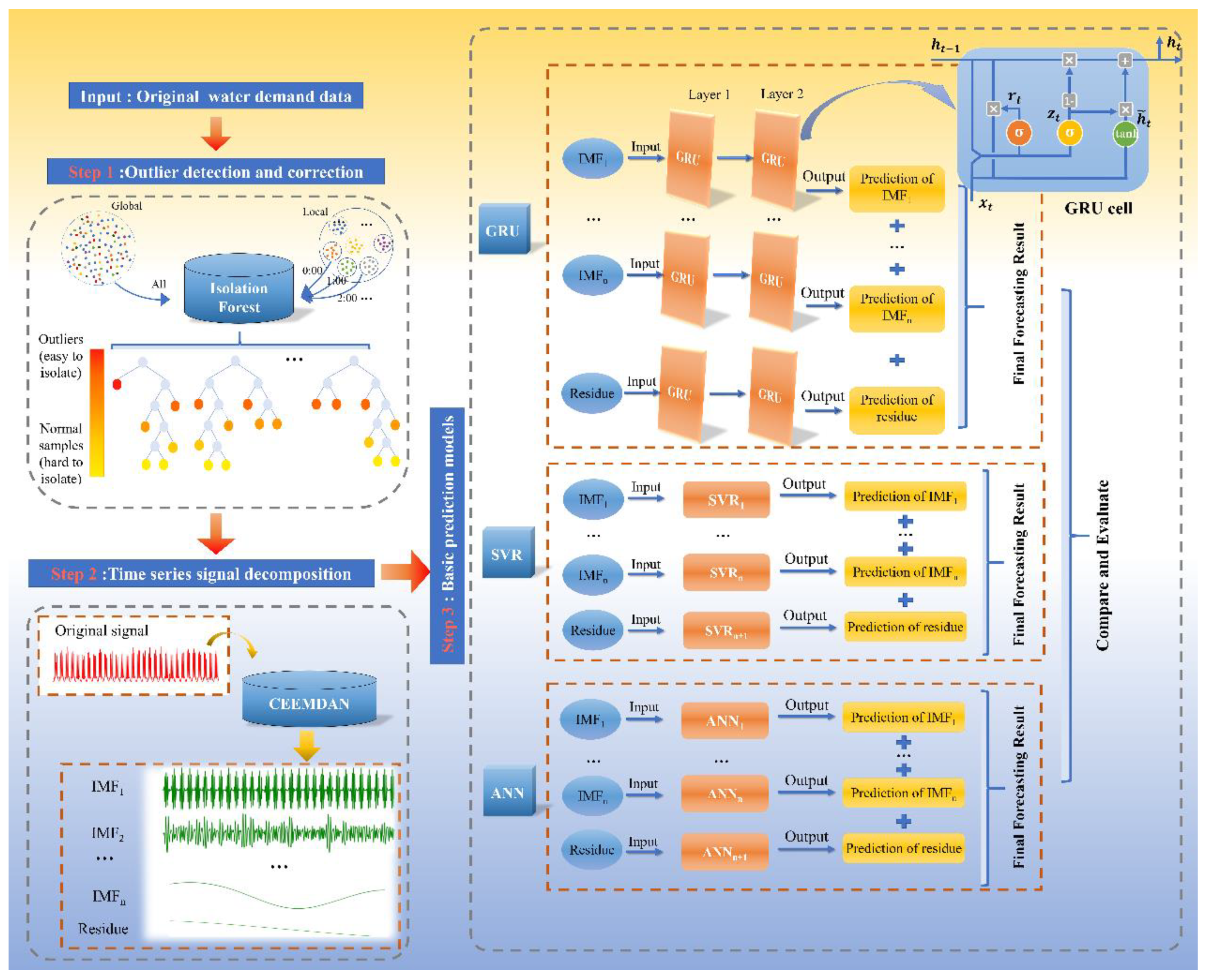
2.6. Research Flowchart

Figure 1 shows the flowchart of the proposed method, and the entire process of this paper is as follows:

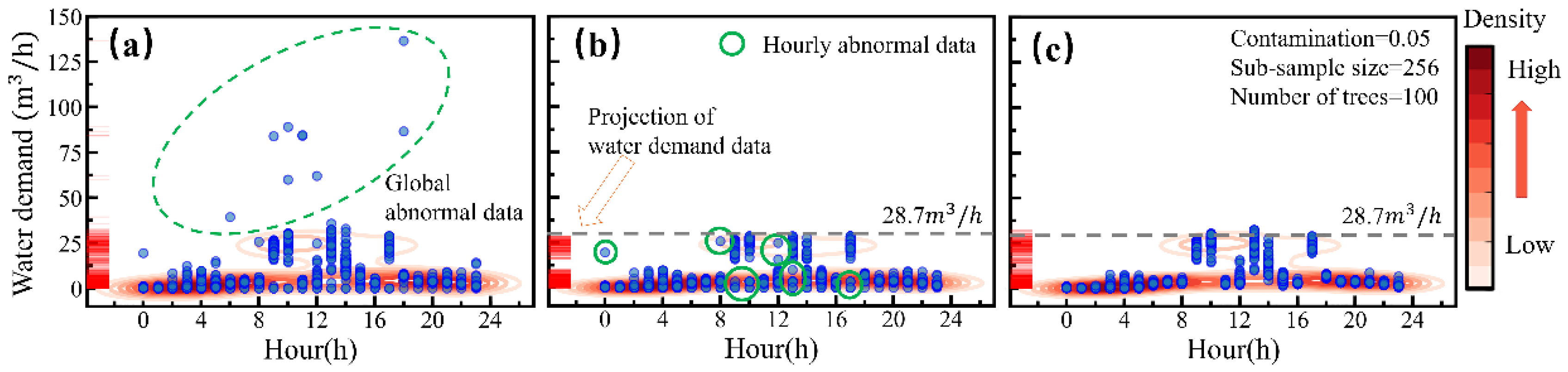
• Through the outlier detection and correction process, the original water demand data are cleaned (i.e., Step 1 in Figure 1). In this study, we have compared the proposed local outlier detection and correction method, and a global outlier detection and correction method. In the local outlier detection and correction method, water demand data are assumed to follow a specific distribution for each hour. First, the water demand data are classified hourly into 24 clusters. Then, 24 Isolation Forest models are built for each cluster to detect the outliers. The outliers are then corrected by the mean value of that hour instead of the global mean value. In the global method, an Isolation Forest model is built based on all the data of water demand, and the outliers are corrected by the global mean value.
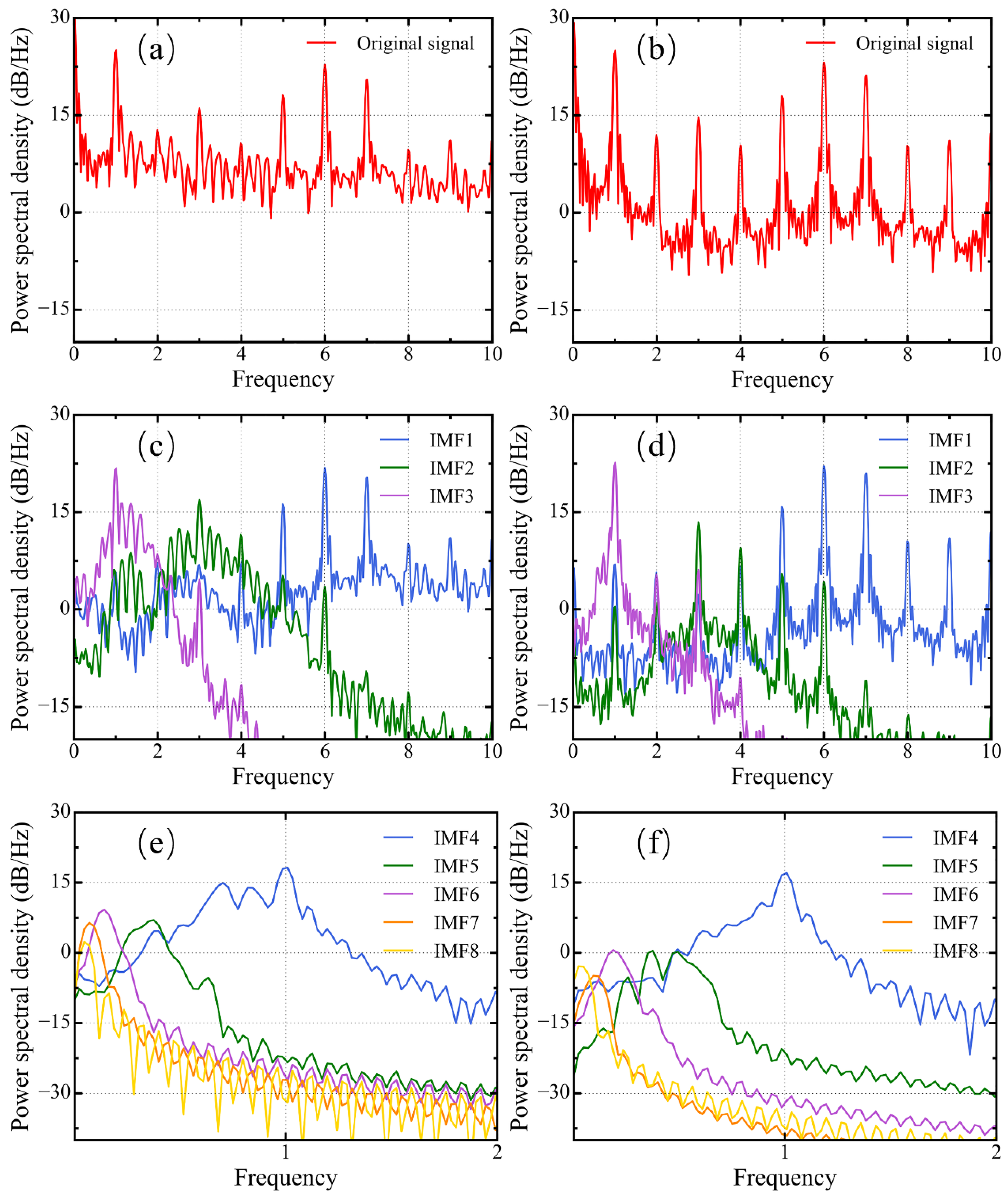
• After outlier correction, the nonstationary and nonlinear time series signal is decomposed adaptively by CEEMDAN and turned into simpler sub-signals (i.e., Step 2 in Figure 1). It is easier for these sub-signals to extract the features.
• The GRU, SVR, and ANN models are built based on each sub-series to explore the efficiency of the proposed preprocessing framework on different forecasting models (i.e., Step 3 in Figure 1). The forecasting result of a water demand time series is the sum of the forecasting results of all the sub-signals.

3. Case Study

3.1. Data Description

As the small- or medium-size data are more sensitive to outliers, in this study, a data set comprising recent time information has been used to investigate the performance of the proposed method. The data set is the hourly water demand data of a DMA in Shanghai, China, from 1 September 2016 to 9 November 2016. The average daily water demand of this area is 170.11 ${\mathrm{m}}^3/\mathrm{d}$. A total of 75% (or 1260 data points) of the water demand data have been used as the training set. Another 15% (or 252 data points) of the data have been used as the validation set to optimize the hyperparameters. The remaining 10% (or 168 data points) have been used as the testing data to evaluate the performance of the models. This study uses the water demand data as the only input, as other meteorological information is usually difficult to obtain for water utilities and previous studies have proved that a single input of water demand history is sufficient for developing accurate models [49,50].

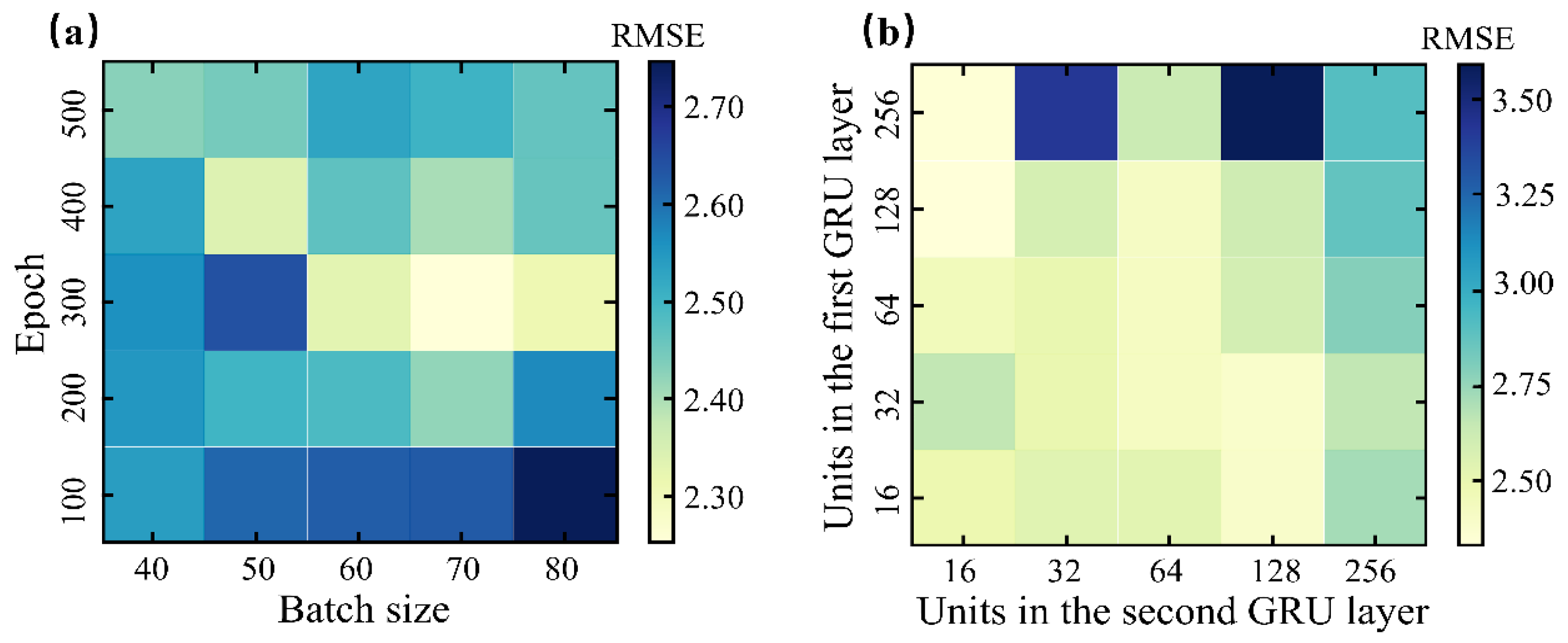
3.2. Model Development

The values of the model hyperparameters determine the performance of the model. Therefore, it is necessary to use the validation set to select the optimal hyperparameters according to the performance of different hyperparameters. The methods of hyperparameter optimization are varied, including Grid Search [51], Genetic Algorithm [52], Particle Swarm Optimization [53], and so on. In this study, we chose Grid Search, which is a commonly used hyperparameter optimization method in water demand forecasting, to optimize the hyperparameters. For the Isolation Forest model, we have tried values from 0.03 to 0.07 with an increment of 0.01 for the hyperparameter of contamination, as shown in Figure S1. The value of the sub-sample size has been set as 256, as this size is big enough to provide information for outlier detection [54]. An earlier study showed that the length of the path converges to an ideal state before 100 trees [39]. Hence, we have set 100 as the number of trees in the Isolation Forest model. The ensemble size I and the amplitude of white noise $\epsilon$ in CEEMDAN have been set as I = 100 and $\epsilon =0.2$, respectively, according to Colominas et al. and Lei et al. [55,56].

The basic forecasting models including the GRU, ANN, and SVR models have been developed to predict the IMFs and the residue. All the input data of the basic forecasting models are first normalized into a range from 0 to 1. The input water demand series comprising $x\left(t-1\right)$, $x\left(t-2\right)$,…$x\left(t-w\right)$ has been used to determine the output $x\left(t\right)$, where $w$ is the window size. We have tried values from 1 to 30 for $w$, as shown in Figure S2, and $w$ = 15 has been set for the GRU, ANN, and SVR forecasting models.

As for the GRU model, there are four important hyperparameters that need to be optimized: (1) Batch size (ranges from 40 to 80, with an increment of 10); (2) epoch (ranges from 100 to 500, with an increment of 100); (3) units in the first GRU layer (i.e., 16, 32, 64, 128, and 256); (4) units in the second GRU layer (i.e., 16, 32, 64, 128, and 256). As the first step, the batch size and epoch have been chosen for the grid search, as shown in Figure 2a. The deeper the blue color, the larger the root-mean-square error (RMSE). As such, the middle right area shows higher accuracy. When the batch size and epoch are set to 70 and 300, respectively, the model achieves the lowest RMSE. As the second step, the hyperparameters of the units in the first and second GRU layers are searched, as shown in Figure 2b. The influence of the units of the GRU layers on the model accuracy is greater than those of the batch size and epoch. The results show that the GRU model does not behave well when the numbers of units for both first and second GRU layers are set to 256. Inversely, the lower left area shows higher accuracy. When the number of units in the first layer is set to 128 and that in the second layer is set to 16, the RMSE is lowest.

For the ANN model, the number of hidden nodes and the initial learning rate need to be optimized. We have tried 2, 5, 7, 10, 20, 30, 40, 50, 60, 70, and 80 for the number of hidden nodes, and 0.0001, 0.001, 0.01, and 0.1 for the initial learning rate. That is, we have tried 44 different combinations of the two hyperparameters for the ANN model.

As for the SVR model, the radial basis function has been chosen as the kernel function, and there are two important hyperparameters, C and gamma, that need to be optimized. C is the hyperparameter of regularization that can adjust the weight of the prediction error and the complexity of the model, and gamma is the kernel coefficient for the radial basis function. We have tried ${\mathrm{e}}^{-2}$, ${\mathrm{e}}^{-1}$, ${\mathrm{e}}^0$, ${\mathrm{e}}^1$, ${\mathrm{e}}^2$, ${\mathrm{e}}^3$, ${\mathrm{e}}^4$, and ${\mathrm{e}}^5$ for the hyperparameter C, and ${\mathrm{e}}^{-4}$, ${\mathrm{e}}^{-3}$, ${\mathrm{e}}^{-2}$, ${\mathrm{e}}^{-1}$, ${\mathrm{e}}^0$, and ${\mathrm{e}}^1$ for the hyperparameter gamma. That is, we have tried 40 different combinations of the two hyperparameters for the SVR model.

3.3. Performance Evaluation Indices

In this study, we have used two absolute error indices (mean absolute error (MAE) and root-mean-square error (RMSE)) and one nondimensional evaluation metric (Nash–Sutcliffe model efficiency coefficient (NSE)) to assess the performance of the forecasting models. Additionally, as forecasting results are supposed to be linear to observed values, the Pearson correlation coefficient (r) has also been used in this study. The indices are defined as:

$$MAE=\frac{1}{N}{\sum }_{i=1}^N\left|Q_i-Q_i^{\prime }\right|,$$

(17)

$$RMSE=\sqrt{\frac{1}{N}{\sum }_{i=1}^N{\left(Q_i-Q_i^{\prime }\right)}^2},$$

(18)

$$NSE=1-\frac{{\sum }_{i=1}^N{\left(Q_i-Q_i^{\prime }\right)}^2}{{\sum }_{i=1}^N{\left(Q_i-\overline{Q_i}\right)}^2},$$

(19)

$$r=\frac{{\sum }_{i=1}^N\left(Q_i-\overline{Q_i}\right)\left(Q_i^{\prime }-\overline{Q_i^{\prime }}\right)}{\sqrt{{\sum }_{i=1}^N{\left(Q_i-\overline{Q_i}\right)}^2{\sum }_{i=1}^N{\left(Q_i^{\prime }-\overline{Q_i^{\prime }}\right)}^2}},$$

(20)

where $Q_i$ is the observed water demand, $Q_i^{\prime }$ is the forecasted water demand, $\overline{Q_i}$ is the mean of the observed water demand, and $\overline{Q_i^{\prime }}$ is the mean of the forecasted water demand. Both MAE and RMSE reflect the deviations between the forecasted and the observed water demands, while the RMSE pays more attention to the large errors. NSE compares the forecasted water demands with the mean of the observed water demand. The Pearson correlation coefficient reflects the strength of the linear relationship between the forecasted and the observed water demands. For the forecasting models with an NSE and Pearson correlation coefficient closer to 1, the forecasts are more accurate.

4. Results and Discussion

This section shows the results and discussion in three aspects. Section 4.1 and Section 4.2 focus on the effect of the proposed preprocessing method. In Section 4.1, the effect of the local outlier detection and correction model is demonstrated. In Section 4.2, the features of the sub-signals after decomposition have been studied. Finally, Section 4.3 explores whether the proposed preprocessing method can improve the accuracy of water demand forecasting.

4.1. Outlier Detection and Correction

Figure 3 shows the original water demand, and the corrected water demand by the global and local outlier detection and correction models. The global abnormal data (Figure 3a) are effectively detected by both methods. Further, the global method has detected few hourly abnormal data (Figure 3b). This is attributed to the subsample function of the Isolation Forest model, which have fewer normal points interfering with the isolation process of abnormal data [57]. However, it is not enough for practical preprocessing engineering of water demand forecasting. The local outlier correction method (Figure 3c) shows great advantages in processing the hourly abnormal data including: (1) Abnormal single points that are overlapped with normal clusters of other hours; (2) abnormal clusters near zero during the peak hours (i.e., 9, 10, 13, and 17 h). Moreover, the local outlier correction method reduces misidentification of the normal samples. For example, the normal points above 28.7 ${\mathrm{m}}^3/\mathrm{h}$ have been misidentified as abnormal data in the global outlier detection and correction method (Figure 3b), while the local detection and correction method has retained these points as normal data according to the distribution of the hourly water demand (Figure 3c). Hence, using the local detection and correction method, more useful information of the raw data will be used for water demand forecasting.

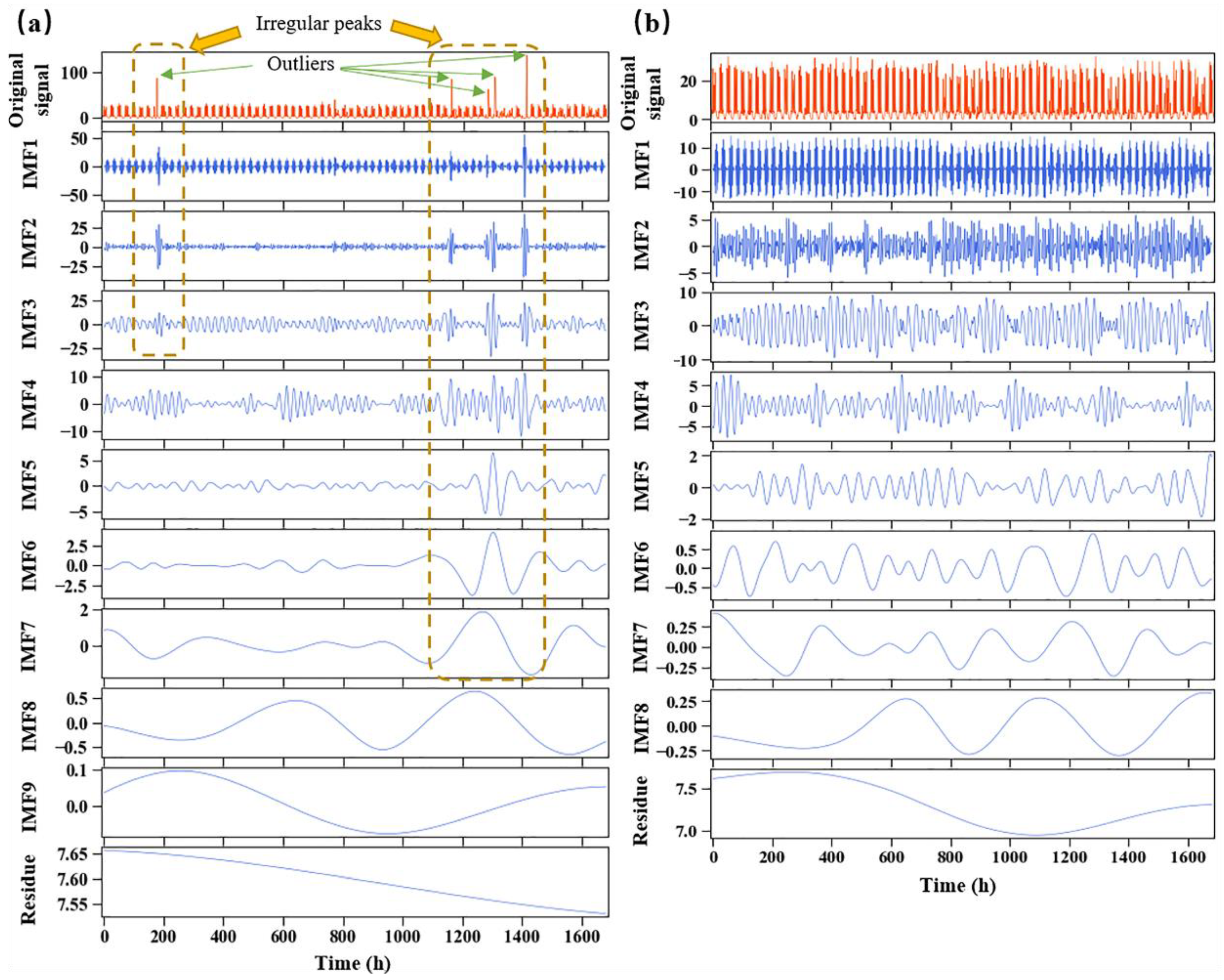
4.2. Time Series Signal Decomposition

Figure 4 shows the results of CEEMDAN including the original signals, the IMFs and the residues of the initial time series (Figure 4a), and the time series processed by the Isolation Forest model (Figure 4b). From Figure 4, it can be seen that the nonstationary and nonlinear original signals have been decomposed by CEEMDAN into several sub-signals, which vary from high frequency to low frequency. The outliers of the initial time series (Figure 4a) have a negative effect on the decomposition process. There are obvious irregular peaks from IMF 1 to IMF 7 caused by the outliers. On the other hand, the IMFs of the time series after outlier correction are smoother and have less signal saltation.

The power spectral densities of the original signal and IMF 1–8 at different levels of frequencies for the time series with and without outlier corrections are shown in Figure 5. The original signals for the original water demand (Figure 5a) and the corrected water demand (Figure 5b) have multiple discrete peaks, resulting in a difficulty in distinguishing the main peak. That is to say, there are strong noise background and different frequency modes in the original signals. On the other hand, each sub-signal of CEEMDAN has an obvious main power spectral density peak. In other words, these sub-signals are more periodic, which makes it easier to capture the signal characteristics for prediction. With the progress of decomposition, the peak moves toward the lower frequency direction and becomes more concentrated. There are several sub-peaks in IMF 1–3, while it is still able to distinguish the main peak. Comparing with IMF 1–3 without Isolation Forest treatment (Figure 5c), the attenuation velocities of the corrected IMFs (Figure 5d) on both sides of the main peak are faster and the kurtosis is more likely to be leptokurtic. IMF 4–8 (Figure 5d,e) can be approximately regarded as unimodal, and the power is concentrated in the peak frequency. The corrected IMFs have less overlap, that is, the characteristic of the signal is well dispersed in the sub-signals.

It can be qualitatively concluded that it is easier to extract the features of the sub-signals processed by CEEMDAN, and the outlier correction method makes a contribution to the efficiency of the decomposition process.

4.3. Overall Performance

With the aim of evaluating the performance of the proposed preprocessing method, and assessing the forecasting performance of different forecasting models, twelve water demand forecasting models have been developed, i.e., SVR, IF-SVR, ANN, IF-ANN, GRU, IF-GRU, CEEMDAN-SVR, IF-CEEMDAN-SVR, CEEMDAN-ANN, IF-CEEMDAN-ANN, CEEMDAN-GRU, and IF-CEEMDAN-GRU. The performance results of these models are shown in

Table 1. Performance results of different models for testing data.

Model	MAE	RMSE	${\mathit{R}}^2$	r
SVR	4.60996	5.58961	0.50343	0.75491
IF-SVR	2.23167	2.95628	0.861099	0.928563
CEEMDAN-SVR	2.60908	3.56389	0.798133	0.904639
IF-CEEMDAN-SVR	1.79512	2.37339	0.910473	0.955239
ANN	2.59636	3.60472	0.793481	0.89321
IF-ANN	2.07612	3.17677	0.839606	0.917693
CEEMDAN-ANN	2.99397	3.99805	0.745954	0.878257
IF-CEEMDAN-ANN	1.9694	2.6012	0.892461	0.945378
GRU	2.27949	3.32249	0.824554	0.910801
IF-GRU	1.98076	3.26109	0.830978	0.916113
CEEMDAN-GRU	1.67429	2.35978	0.911497	0.957639
IF-CEEMDAN-GRU	1.52313	2.32435	0.914134	0.956688

.

Firstly, to verify the importance of the proposed hybrid preprocessing method, the first groups of comparisons are SVR vs. IF-CEEMDAN-SVR, ANN vs. IF-CEEMDAN-ANN, and GRU vs. IF-CEEMDAN-GRU. According to Table 1, the basic forecasting models combined with IF-CEEMDAN can achieve higher accuracy of prediction. For example, the RMSEs of IF-CEEMDAN-SVR, IF-CEEMDAN-ANN, and IF-CEEMDAN-GRU have reduced by 57.5%, 27.8%, and 30.0% as compared to those of SVR, ANN, and GRU, respectively. Therefore, according to Section 4.1 and Section 4.2, the sub-signals whose features are easier to extract contribute to improving the performance of the forecasting.

Secondly, besides CEEMDAN-ANN, all the other single preprocessing technique-based models, i.e., IF-SVR, IF-ANN, IF-GRU, CEEMDAN-SVR, and CEEMDAN-GRU, have improved the accuracy of the basic forecasting models, as shown in Table 1. For instance, the MAE of CEEMDAN-SVR and IF-SVR have reduced from 4.61 to 2.61 ${\mathrm{m}}^3/\mathrm{h}$ and from 4.61 to 2.23 ${\mathrm{m}}^3/\mathrm{h}$, respectively. The exception of CEEMDAN-ANN may be due to the overfitting problem of ANN. The overfitting problem makes ANN susceptible to outliers. According to Section 4.2, the outliers cause irregular peaks in the IMFs. Hence, the prediction accuracy can be influenced by the overfitting problem of ANN and the error has been accumulated in the decomposition and integration process of CEEMDAN, which makes the performance of CEEMDAN-ANN inferior to the ANN model.

Thirdly, from Table 1, it can be seen that the GRU-based models are superior to the other models due to its excellent feature extraction ability. The IF-CEEMDAN-GRU obtains a minimum RMSE of 2.32 ${\mathrm{m}}^3/\mathrm{h}$ among the twelve water demand forecasting models. Even the GRU without the preprocessing technique can achieve similar or even better performance than the ANN and SVR models with a single preprocessing technique. The GRU method shows great potential in water demand forecasting. Additionally, it is worth noting that although the SVR model has a disappointing result, the IF-CEEMDAN-SVR can achieve an accuracy close to that of IF-CEEMDAN-GRU.

To investigate how the outlier correction and signal decomposition methods improve the accuracy of water demand prediction intuitively, the profiles of the predicted and observed water demand time series are shown in Figure 6. According to Figure 6d, the predictions by the IF-CEEMDAN-based models are closer to the observed water demand curve. The IF-based models can improve the accuracy of the water demand predictions during the nonpeak period, as shown in Figure 6b. On the other hand, the CEEMDAN-based models (Figure 6c) show better performance at peak hours, especially for the peaks between 80 and 120 h. It can be inferred that Isolation Forest and CEEMDAN supplement each other throughout the whole water demand time series.

Additionally, the computation time has been used to quantify the forecasting speed, as shown in

Table 2. Comparison of CPU time for different models.

Model	CPU Time (s)	Model	CPU Time (s)
SVR	0.008	CEEMDAN-SVR	13.579
IF-SVR	3.584	IF-CEEMDAN-SVR	17.134
ANN	0.075	CEEMDAN-ANN	14.641
IF-ANN	3.668	IF-CEEMDAN-ANN	18.529
GRU	192.128	CEEMDAN-GRU	1934.022
IF-GRU	194.508	IF-CEEMDAN-GRU	1996.464

. The computer environment is AMD Ryzen5 3600 CPU at 3.60 GHz and NVIDIA GeForce RTX 2060 SUPER GPU at 1695 MHz equipped with Python 3.6.9. As shown in Table 2, the CPU Times used by the GRU-based models are much longer than those by the ANN and SVR models. This indicates that the structure of the GRU-based models is more complex and hence leads to a higher computational load. Although the GRU-based models need more computational time, they can achieve superior prediction performance. Besides the GRU-based model, IF-CEEMDAN-SVR is a noteworthy model that can achieve an accuracy close to that of IF-CEEMDAN-GRU and requires less CPU time.

5. Conclusions

In this study, the potential of the preprocessing process in hourly water demand forecasting has been investigated. For the first time, the outlier detection and correction model Isolation Forest, and the adaptive signal decomposition technique CEEMDAN have been introduced to water demand forecasting. Moreover, a promising deep learning method of GRU, which has an excellent feature extraction ability for time series, has been used as a basic forecasting model. The results have been compared with those of ANN and SVR to investigate the efficiency of the proposed preprocessing framework on different models. Combining the advantages of the two preprocessing methods, the hybrid IF-CEEMDAN-based models have been developed for hourly water demand forecasting, which can produce high accuracy in predictions. The conclusions of this study are as follows:

• The proposed preprocessing method can greatly improve the accuracy of hourly water demand forecasting models. The RMSE of the SVR, ANN, and GRU models has reduced by 57.5%, 27.8%, and 30.0%, respectively.
• The local outlier detection and correction method not only effectively identifies global outlier and outlier clusters that are overlapped with other normal data, but also reduce misidentification of normal samples.
• The CEEMDAN model is able to decompose nonstationary and nonlinear water demand time series into sub-signals with an obvious main power spectral density peak, which makes it easier to capture the signal characteristics for prediction.
• Despite the higher computational load, the GRU-based models always perform better than the ANN and SVR-based models. The IF-CEEMDAN-GRU model is the most accurate model among the twelve models examined in this study. The prediction by the SVR model without preprocessing is poor, but the IF-CEEMDAN-SVR model can achieve an accuracy close to that of the IF-CEEMDAN-GRU model with lower computational load. That is, the proposed method can also exert great potential on some of the conventional models.

In the practical engineering of hourly water demand forecasting, the proposed hybrid preprocessing method has great superiority in predicting complex nonstationary hourly water demand time series, which is vital for pump schedule, energy conservation, and leakage reduction. Hence, the proposed method has great potential to help to achieve sustainable operation and cost-effective management of water distribution networks.

Future work should test other preprocessing techniques to further improve the performance of hourly water demand forecasting models, and test the water demand of different cities to explore the stability of the framework. Moreover, due to the lack of information about abnormal events that cause the outliers, this paper can only identify the outliers rather than distinguishing the abnormal events. Future studies can focus on identifying the abnormal events of outliers after collecting more information, and achieve additional functions such as leakage detection.

References

1. Hao, L.; Sun, G.; Liu, Y.; Qian, H. Integrated Modeling of Water Supply and Demand under Management Options and Climate Change Scenarios in Chifeng City, China. JAWRA J. Am. Water Resour. Assoc. 2015, 51, 655–671. [Google Scholar] [CrossRef]
2. Kifle Arsiso, B.; Mengistu Tsidu, G.; Stoffberg, G.H.; Tadesse, T. Climate change and population growth impacts on surface water supply and demand of Addis Ababa, Ethiopia. Clim. Risk Manag. 2017, 18, 21–33. [Google Scholar] [CrossRef]
3. Adamowski, J.; Fung Chan, H.; Prasher, S.O.; Ozga-Zielinski, B.; Sliusarieva, A. Comparison of multiple linear and nonlinear regression, autoregressive integrated moving average, artificial neural network, and wavelet artificial neural network methods for urban water demand forecasting in Montreal, Canada. Water Resour. Res. 2012, 48. [Google Scholar] [CrossRef]
4. Donkor, E.A.; Mazzuchi, T.A.; Soyer, R.; Roberson, J.A. Urban Water Demand Forecasting: Review of Methods and Models. J. Water Resour. Plan. Manag. 2014, 140, 146–159. [Google Scholar] [CrossRef]
5. Polebitski, A.S.; Palmer, R.N. Seasonal Residential Water Demand Forecasting for Census Tracts. J. Water Resour. Plan. Manag. 2010, 136, 27–36. [Google Scholar] [CrossRef]
6. Francesca, G.; Stefano, A.; Zoran, K.; Marco, F. A probabilistic short-termwater demand forecasting model based on the Markov chain. Water 2017, 9, 507. [Google Scholar]
7. Duerr, I.; Merrill, H.R.; Wang, C.; Bai, R.; Boyer, M.; Dukes, M.D.; Bliznyuk, N. Forecasting urban household water demand with statistical and machine learning methods using large space-time data: A Comparative study. Environ. Model. Softw. 2018, 102, 29–38. [Google Scholar] [CrossRef]
8. McKenna, S.A.; Fusco, F.; Eck, B.J. Water Demand Pattern Classification from Smart Meter Data. Procedia Eng. 2014, 70, 1121–1130. [Google Scholar] [CrossRef] [Green Version]
9. Mamade, A.; Loureiro, D.; Covas, D.; Coelho, S.T.; Amado, C. Spatial and Temporal Forecasting of Water Consumption at the DMA Level Using Extensive Measurements. Procedia Eng. 2014, 70, 1063–1073. [Google Scholar] [CrossRef] [Green Version]
10. Seok, J.; Kim, J.; Lee, J.; Lee, J.; Song, Y.; Shin, G. Abnormal data refinement and error percentage correction methods for effective short-term hourly water demand forecasting. Int. J. Control Autom. 2014, 12, 1245–1256. [Google Scholar] [CrossRef]
11. De Souza Groppo, G.; Costa, M.A.; Libânio, M. Predicting water demand: A review of the methods employed and future possibilities. Water Supply 2019, 19, 2179–2198. [Google Scholar] [CrossRef]
12. Adamowski, J.F. Peak Daily Water Demand Forecast Modeling Using Artificial Neural Networks. J. Water Resour. Plan. Manag. 2008, 134, 119–128. [Google Scholar] [CrossRef] [Green Version]
13. Caiado, J. Performance of Combined Double Seasonal Univariate Time Series Models for Forecasting Water Demand. J. Hydrol. Eng. 2010, 15, 215–222. [Google Scholar] [CrossRef] [Green Version]
14. Oyebode, O.; Ighravwe, D.E. Urban Water Demand Forecasting: A Comparative Evaluation of Conventional and Soft Computing Techniques. Resources 2019, 8, 156. [Google Scholar] [CrossRef] [Green Version]
15. Shvartser, L.; Shamir, U.; Feldman, M. Forecasting Hourly Water Demands by Pattern Recognition Approach. J. Water Resour. Plan. Manag. 1993, 119, 611–627. [Google Scholar] [CrossRef]
16. Arandia, E.; Ba, A.; Eck, B.; McKenna, S. Tailoring Seasonal Time Series Models to Forecast Short-Term Water Demand. J. Water Resour. Plan. Manag. 2016, 142, 4015067. [Google Scholar] [CrossRef] [Green Version]
17. Adamowski, J.; Karapataki, C. Comparison of Multivariate Regression and Artificial Neural Networks for Peak Urban Water-Demand Forecasting: Evaluation of Different ANN Learning Algorithms. J. Hydrol. Eng. 2010, 15, 729–743. [Google Scholar] [CrossRef] [Green Version]
18. Herrera, M.; Torgo, L.; Izquierdo, J.; Pérez-García, R. Predictive models for forecasting hourly urban water demand. J. Hydrol. 2010, 387, 141–150. [Google Scholar] [CrossRef]
19. Ghalehkhondabi, I.; Ardjmand, E.; Weckman, G.; Young, W. Water Demand Forecasting: Review of Soft Computing Methods. Environ. Monit. Assess. 2017, 189, 313. [Google Scholar] [CrossRef]
20. Bougadis, J.; Adamowski, K.; Diduch, R. Short-term municipal water demand forecasting. Hydrol. Process. 2005, 19, 137–148. [Google Scholar] [CrossRef]
21. Ghiassi, M.; Zimbra, D.K.; Saidane, H. Urban Water Demand Forecasting with a Dynamic Artificial Neural Network Model. J. Water Resour. Plan. Manag. 2008, 134, 138–146. [Google Scholar] [CrossRef]
22. Fei, S.; He, Y. Wind speed prediction using the hybrid model of wavelet decomposition and artificial bee colony algorithm-based relevance vector machine. Int. J. Electr. Power Energy Syst. 2015, 73, 625–631. [Google Scholar] [CrossRef]
23. Shen, C. A Transdisciplinary Review of Deep Learning Research and Its Relevance for Water Resources Scientists. Water Resour. Res. 2018, 54, 8558–8593. [Google Scholar] [CrossRef]
24. Guo, G.; Liu, S.; Wu, Y.; Li, J.; Zhou, R.; Zhu, X. Short-Term Water Demand Forecast Based on Deep Learning Method. J. Water Resour. Plan. Manag. 2018, 144, 04018076. [Google Scholar] [CrossRef]
25. Ren, Z.; Li, S. Short-term demand forecasting for distributed water supply networks: A multi-scale approach. In Proceedings of the 2016 12th World Congress on Intelligent Control and Automation (WCICA), Guilin, China, 12–15 June 2016; pp. 1860–1865. [Google Scholar]
26. Wu, Z.; Huang, N.E. Ensemble Empirical Mode Decomposition: A Noise-Assisted Data Analysis Method. Adv. Adapt. Data Anal. 2009, 1, 1–41. [Google Scholar] [CrossRef]
27. Deng, X.; Hou, S.; Li, W.; Liu, X. Hourly Campus Water Demand Forecasting Using a Hybrid. EEMD-Elman Neural Network Model; Dong, W., Lian, Y., Zhang, Y., Eds.; Springer International Publishing: Cham, Switzerland, 2019; pp. 71–80. [Google Scholar]
28. Himeur, Y.; Ghanem, K.; Alsalemi, A.; Bensaali, F.; Amira, A. Artificial intelligence based anomaly detection of energy consumption in buildings: A review, current trends and new perspectives. Appl. Energy 2021, 287, 116601. [Google Scholar] [CrossRef]
29. Santos, F. Modern methods for old data: An overview of some robust methods for outliers detection with applications in osteology. J. Archaeol. Sci. Rep. 2020, 32, 102423. [Google Scholar] [CrossRef]
30. Zheng, S.; Zhu, Y.X.; Li, D.Q.; Cao, Z.J.; Phoon, K.K. Probabilistic outlier detection for sparse multivariate geotechnical site investigation data using Bayesian learning. Geosci. Front. 2020, 12, 425–439. [Google Scholar] [CrossRef]
31. Van Capelleveen, G.; Poel, M.; Mueller, R.M.; Thornton, D.; Van Hillegersberg, J. Outlier detection in healthcare fraud: A case study in the Medicaid dental domain. Int. J. Account. Inf. Syst. 2016, 21, 18–31. [Google Scholar] [CrossRef]
32. Michalak, M.; Wawrowski, U.; Sikora, M.; Kurianowicz, R.; Bialas, A. Outlier Detection in Network Traffic Monitoring. In Proceedings of the 10th International Conference on Pattern Recognition Applications and Methods (ICPRAM 2021), Vienna, Austria, 4–6 February 2021. [Google Scholar]
33. Laurikkala, J.; Juhola, M.; Kentala, E. Informal Identification of Outliers in Medical Data. In Proceedings of the Fifth International Workshop on Intelligent Data Analysis in Medicine and Pharmacology, Berlin, Germany, 22 August 2000. [Google Scholar]
34. Rousseeuw, P.J.; Driessen, K.V. Computing LTS Regression for Large Data Sets. Data Min. Knowl. Discov. 2006, 12, 29–45. [Google Scholar] [CrossRef] [Green Version]
35. Zhang, K.; Hutter, M.; Jin, H. A New Local Distance-Based Outlier Detection Approach for Scattered Real-World Data. In Pacific-asia Conference on Knowledge Discovery & Data Mining; Springer: Berlin/Heidelberg, Germany, 2009. [Google Scholar]
36. Breunig, M.; Kriegel, H.; Ng, R.; Sander, J. LOF: Identifying Density-Based Local Outliers. In Proceedings of the 2000 ACM SIGMOD International Conference on Management of Data, Dallas, TX, USA, 16–18 May 2000; Volume 29, pp. 93–104. [Google Scholar]
37. Smiti, A. A critical overview of outlier detection methods. Comput. Sci. Rev. 2020, 38, 100306. [Google Scholar] [CrossRef]
38. Chan, T.K.; Chin, C.S. Unsupervised Bayesian Nonparametric Approach with Incremental Similarity Tracking of Unlabeled Water Demand Time Series for Anomaly Detection. Water 2019, 11, 2066. [Google Scholar] [CrossRef] [Green Version]
39. Liu, F.T.; Ting, K.M.; Zhou, Z.H. Isolation Forest. In Proceedings of the 2008 Eighth IEEE International Conference on Data Mining, Pisa, Italy, 15–19 December 2008. [Google Scholar]
40. Huang, N.E.; Shen, Z.; Long, S.R.; Wu, M.C.; Shih, H.H.; Zheng, Q.; Yen, N.; Tung, C.C.; Liu, H.H. The empirical mode decomposition and the Hilbert spectrum for nonlinear and non-stationary time series analysis. Proc. R. Soc. Lond. Ser. A Math. Phys. Eng. Sci. 1998, 454, 903–995. [Google Scholar] [CrossRef]
41. Torres, M.E.; Colominas, M.A.; Schlotthauer, G.; Flandrin, P. A complete ensemble empirical mode decomposition with adaptive noise. In Proceedings of the 2011 IEEE International Conference on Acoustics, Speech and Signal Processing (ICASSP), Prague, Czech Republic, 22–27 May 2011; pp. 4144–4147. [Google Scholar]
42. Seo, Y.; Kwon, S.; Choi, Y. Short-Term Water Demand Forecasting Model Combining Variational Mode Decomposition and Extreme Learning Machine. Hydrology 2018, 5, 54. [Google Scholar] [CrossRef] [Green Version]
43. Cho, K.; van Merriënboer, B.; Bahdanau, D.; Bengio, Y. On the Properties of Neural Machine Translation: Encoder-Decoder Approaches. arXiv 2014, arXiv:1409.1259. [Google Scholar]
44. Pesantez, J.E.; Berglund, E.Z.; Kaza, N. Smart meters data for modeling and forecasting water demand at the user-level. Environ. Model. Softw. 2020, 125, 104633. [Google Scholar] [CrossRef]
45. Antonio, C. Clustering and Support Vector Regression for Water Demand Forecasting and Anomaly Detection. Water 2017, 9, 224. [Google Scholar]
46. Candelieri, A.; Archetti, F. Identifying Typical Urban Water Demand Patterns for a Reliable Short-term Forecasting—The Icewater Project Approach. Procedia Eng. 2014, 89, 1004–1012. [Google Scholar] [CrossRef] [Green Version]
47. Candelieri, A.; Giordani, I.; Archetti, F.; Barkalov, K.; Meyerov, I.; Polovinkin, A.; Sysoyev, A.; Zolotykh, N. Tuning hyperparameters of a SVM-based water demand forecasting system through parallel global optimization. Comput. Oper. Res. 2018, 106, 202–209. [Google Scholar] [CrossRef]
48. Bernhard Scholkopf, A.J.S. Learning with Kernels: Support Vector Machines, Regularization, Optimization, and Beyond; Adaptive Computation and Machine Learning Series; The MIT Press: Cambridge, MA, USA, 2018. [Google Scholar]
49. Bakker, M.; Vreeburg, J.H.G.; van Schagen, K.M.; Rietveld, L.C. A fully adaptive forecasting model for short-term drinking water demand. Environ. Model. Softw. 2013, 48, 141–151. [Google Scholar] [CrossRef]
50. Alvisi, S.; Franchini, M.; Marinelli, A. A short-term, pattern-based model for water-demand forecasting. J. Hydroinform. 2007, 9, 39–50. [Google Scholar] [CrossRef] [Green Version]
51. Carriero, A.; Kapetanios, G.; Marcellino, M. Forecasting large datasets with Bayesian reduced rank multivariate models. J. Appl. Econ. 2011, 26, 735–761. [Google Scholar] [CrossRef] [Green Version]
52. Zhou, Z.; Xiong, F.; Huang, B.; Xu, C.; Jiao, R.; Liao, B.; Yin, Z.; Li, J. Game-Theoretical Energy Management for Energy Internet With Big Data-Based Renewable Power Forecasting. IEEE Access 2017, 5, 5731–5746. [Google Scholar] [CrossRef]
53. Raza, M.Q.; Nadarajah, M.; Ekanayake, C. Demand forecast of PV integrated bioclimatic buildings using ensemble framework. Appl. Energy 2017, 208, 1626–1638. [Google Scholar] [CrossRef]
54. Ding, Z.; Fei, M. An Anomaly Detection Approach Based on Isolation Forest Algorithm for Streaming Data using Sliding Window. IFAC Proc. Vol. 2013, 46, 12–17. [Google Scholar] [CrossRef]
55. Colominas, M.A.; Schlotthauer, G.; Torres, M.E. Improved complete ensemble EMD: A suitable tool for biomedical signal processing. Biomed. Signal Process. Control 2014, 14, 19–29. [Google Scholar] [CrossRef]
56. Lei, Y.; Liu, Z.; Ouazri, J.; Lin, J. A fault diagnosis method of rolling element bearings based on CEEMDAN. Proc. Inst. Mech. Eng. Part C J. Mech. Eng. Sci. 2015, 231, 1804–1815. [Google Scholar] [CrossRef]
57. Liu, F.T.; Ting, K.; Zhou, Z. Isolation-Based Anomaly Detection. ACM Trans. Knowl. Discov. Data TKDD 2012, 6, 1–39. [Google Scholar] [CrossRef]
Figure 1. The flowchart of the proposed method including outlier detection and correction, time series signal decomposition, and basic forecasting models.
Water 13 00582 g001
Figure 2. The parametric heatmap for (a) batch size and epoch, and (b) the numbers of units in the first layer and the second layer of the Gated Recurrent Unit (GRU) models.
Water 13 00582 g002
Figure 3. Scatter and density contour map of (a) the observed water demand; (b) the results of global outlier detection and correction; (c) the results of local outlier detection and correction. Blue scatters represent the hourly water demand data in different hours. The right color bar shows the density contour map for water demand data. Red lines near the y-axis are the projections of water demand data.
Water 13 00582 g003
Figure 4. Original signals, their corresponding Intrinsic Mode Functions (IMFs), and residue results of Complete Ensemble Empirical Mode Decomposition with Adaptive Noise (CEEMDAN) for (a) initial time series, and (b) time series processed by Isolation Forest.
Water 13 00582 g004
Figure 5. Spectra of (a) original signal, (c) IMF 1–3, and (e) IMF 4–8 of initial time series and spectra of (b) original signal, (d) IMF 1–3, and (f) IMF 4–8 of time series processed by Isolation Forest.
Water 13 00582 g005
Figure 6. Water demand forecasting results of: (a) GRU, Artificial Neural Network (ANN), and Support Vector Regression (SVR); (b) Isolation Forest (IF)-GRU, IF-ANN, and IF-SVR; (c) CEEMDAN-GRU, CEEMDAN-ANN, and CEEMDAN-SVR; and (d) IF-CEEMDAN-GRU, IF-CEEMDAN-ANN, and IF-CEEMDAN-SVR.
Water 13 00582 g006