
Water Leak Localization Using High-Resolution Pressure Sensors


Faculty of Civil and Environmental Engineering, Technion—Israel Institute of Technology, Haifa 32000, Israel
*
Author to whom correspondence should be addressed.
Water 2021, 13(5), 591; https://doi.org/10.3390/w13050591
Submission received: 22 January 2021
/
Revised: 19 February 2021
/
Accepted: 19 February 2021
/
Published: 25 February 2021
(This article belongs to the Section Hydraulics and Hydrodynamics)
Abstract
:A new method for identifying a leaking pipe within a pressurized water distribution system is presented. This novel approach utilizes transient modeling to analyze water networks. Urban water supply networks are important infrastructure that ensures the daily water consumption of urban residents and industrial sites. The aging and deterioration of drinking water mains is the cause of frequent burst pipes, thus making the detection and localization of these bursts a top priority for water distribution companies. Here we describe a novel method based on transient modeling of the water network and produces high-resolution pressure response under various scenarios. Analyzing this data allows the prediction of the leaking pipe. The transient pressure data is classified as leaking pipes or no leak clusters using the K-nearest neighbors (K-NN) algorithm. The transient model requires a massive computation effort to simulate the network’s performance. The classification model presented good performance with an overall accuracy of 0.9 for the basic scenarios. The lowest accuracy was obtained for interpolated scenarios the model had not been trained on; in this case, the accuracy was 0.52.
1. Introduction
Many water distribution systems lose a significant amount of water as a result of leaks in the distribution pipes [1]. Studies indicate that 15–35% of the potable water supply in the United States, 6.5–25% in Europe, and 4–27% in Korea is lost in the form of non-revenue water. A leak in a water network is typically characterized by a weak flow hidden in the background flow, while water pipe bursts are often identified by a flow change or pressure drop [2]. Most water supply lines are buried underground, making leaks difficult to detect and locate [3]. Water leaking from buried pipes is an increasing concern because of changes in rainfall patterns and the ever-increasing water demand [4]. To tackle this challenge of detecting and locating leaks, some works examined the best locations of the sensors [5], while others developed sensors to monitor parameters in water grids. Rocher et al. [6] suggested an inductive sensor for monitoring the water level in tubes of water distribution systems grids, based on measuring changes in the sensor magnetic field. Zhang et al. [7] introduced a self-powered water level sensor for the marine industry using a liquid–solid tubular triboelectric nanogenerator (LST-TENG). Both sensors can potentially be adapted for sensitive measurements of water distribution systems’ storage levels which are important in the overall analysis of transients in water systems [6].
Recent technological progress makes it possible for water utilities to collect increasing amounts of data from water distribution systems via loggers and telemetry systems [8]. Analyzing the data accumulated can contribute to making the water network more reliable and efficient. Kühnert et al. [9] applied principal component analysis to detect anomalies in the streaming data gained by water distribution network (WDN) sensors. Aminravan et al. [10] suggested a hierarchical rule-based approach to account for the spatial nature of occurrences in WDNs. Stephens et al. [11] applied acoustic signal processing to detect water leaks in city networks. Other methods used a multistage approach combining hydraulic modeling with mathematical analysis. Steffelbauer et al. [12] used dual network with a genetic algorithm (GA). Li et al. [13] used a gradient-based algorithm for model calibration, then cluster leak candidates using the K-means algorithm. Machine-learning-based methods were also used for the purpose of leak detection. Izquierdo et al. [14] assessed anomalies utilizing a hybrid model composed of a deterministic part (flow rates and head at the nodes) coupled with a state estimation technique and artificial neural networks (ANN). Zhang et al. [15] used the K-means algorithm to classify the water network into several zones and then used support vector machine (SVM) to locate the zones containing the leakages. Another approach suggested by Fang et al. [16] is a prediction of leakage events with a convolutional neural network (CNN) dependent on historical data. The methods described above focused on standard pressure data, whether modeled or measured. A new approach is suggested here. It includes generating high-resolution pressure data using TSnet, a novel transient water network modeling application [17]. Then, analyze the data to represent the WDN response to the modeled transient scenarios. It is expected that the high-resolution data, resulting from transient modeling, will reveal patterns that cannot be recognized in the standard pressure measured data. The generation of an artificial high-resolution database might reveal other opportunities for improvement in WDN operation and reliability.
This study consists of two main parts. The first part is the transient model of WDN. This part is described in the Materials and Methods section as Database Formation. The second part classifies the database sampled events. This part is described in the Materials and Methods section as Data Analysis and Classification Algorithm.
2. Materials and Methods
Leak location modeling requires generating a database that represents a transient state of a specific water network under various consumption load configurations, water leak locations, and magnitudes. To evaluate the water network reaction to a specific leak scenario, a transient model is required. Here, we used TSnet version 0.1.2 written in Python [18]. Since the data are not dependent on external measurements, we were able to model leaks in a range of leak diameters, demand configurations, and leak locations in the network. Using this transient model, we established a database representing the network’s pressure response to the leakages’ scenario space. The data consisted of high-resolution pressure values series, each labeled by the pipe’s ID, the distance from the pipe’s start, and the leak diameter. To utilize this dataset in favor of the leak localization model, a machine learning algorithm was used. There are several machine learning classification algorithms appropriate for this task, such as K-nearest neighbors (K-NN), SVM, Random Forest, etc. Here, K-NN was used to predict the leaks in the pipes according to the pressure observed in the network.
2.1. Database Formation
Database creation took place in two steps. Step 1, simulated leak location and diameter were defined. Step 2 consisted of a hydraulic transient simulation of the water network incorporating the newly defined leak. To simulate water leakage from a specific pipe and its location, the network must be reconfigured to generate a node at the leak’s defined location. To form the node in the right place, we first selected which pipe we wanted to leak. Then we used the EPANET python wrapper WNTR version 0.2.1 [19] to obtain the start and end nodes of this pipe and their locations. The new node was configured by stating its location between the start and end nodes with a distance from the start node that matched our decision. The new node was connected to the network with new pipes that replaced the original one. When designating a new node as a leak, the leak properties need to be defined as stipulated in TSnet. In the TSnet model, the leak discharge is defined by using the orifice plate equation (Equation (1)):
where Ql is the leak discharge, k is the leak constant, and H is the pressure head at the leak node. This equation, however, is not specific enough because it does not include information on the leak diameter. To overcome this, we used Crowl and Louvar’s leakage equation [20] (Equation (2)):
where Ql is the leak discharge, Cd is the discharge coefficient, and for turbulent flow taken as Cd = 0.75, D is the leak diameter, p is the gauge water pressure inside the pipe, α is the discharge coefficient, where α = 0.5 assuming a steel pipe with a large hole and ρ is the density of the fluid. To simplify Equation (2), we used the pressure head definition (Equation (3)):
where H is the head, p is the liquid pressure, ρ is the density of the fluid, and g is the gravity acceleration. Manipulating Equations (1)–(3) defines the leak constant k in terms of the leak diameter (Equation (4)):
Next, we defined the transient simulation as a pressure-driven demand (PDD) and ran the simulation. In our database, all leaks started at the same time during the simulation (10 s after the simulation began) and developed over the same period (1 s). Our simulation modeled five minutes of network function. The size of the database depended on the network configuration, the number of load configurations applied, the distance between the simulated leaks, the number of leak sizes, and the sampling resolution. When building the database, each run simulated a specific leaking pipe, its location along the pipe, and the leak diameter. The model iterated through every location and diameter combination to produce the full network scenario simulations. After each simulation, the pressure heads from all of the nodes were saved to the database.
2.2. Data Analysis
The database consisted of a time series of the pressure measured at the network’s nodes. The length of the series depended on the duration of the simulation and the sampling resolution. The database structure is presented in Table 1.
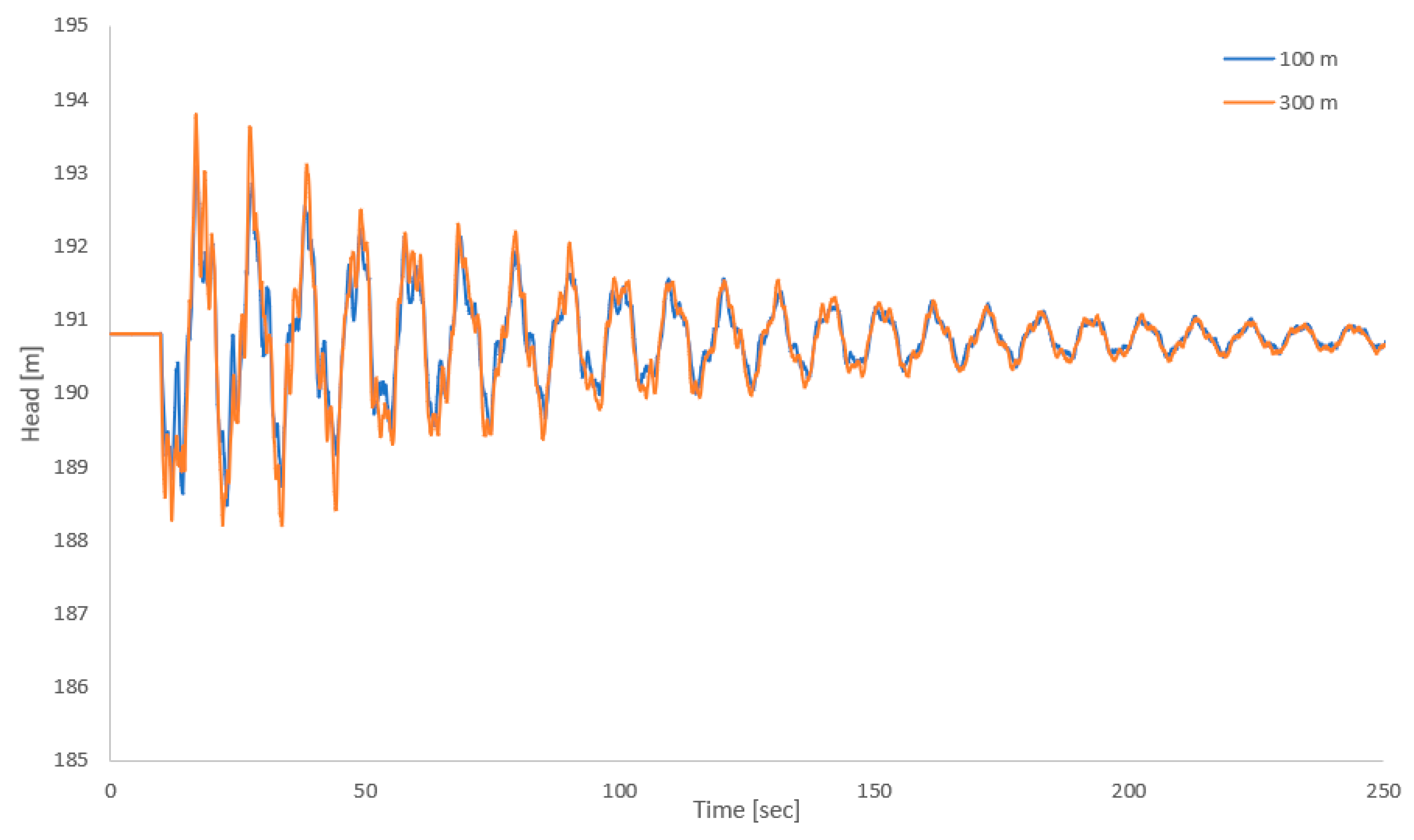
Before the computer-based data analysis, an intuitive evaluation of the impact of different leaks on the water network was conducted. Figure 1 presents the impact of a leak with a 5 mm diameter on the measured head at the neighbor node. This figure shows the impact of shifting the leak 200 m on the same pipe from 100 m from the pipe’s start to 300 m from the pipe’s start. It clearly depicts the amplitude difference caused by the different leak locations. Although the pattern of the main shock wave was very similar in both leak locations, the small waves on top acted very differently from one another. Looking at the figure, one can see that the blue and orange lines were acting similarly, while they were not located exactly one on top of the other. The reason for them not to be exactly on top of each other is the small waves on top and the time difference between the shock wave arrival.
This kind of analysis proves that using a proper computerized analysis might be possible to predict leaks in a pipe. However, to make the simulation more realistic, the measured heads were noised by a factor correlated to the head at the node before the leak burst. In real water networks, the pressures are never steady due to changes in demands, the water level at the tanks, pumps trembling, etc. The purpose of the noise added to the measured pressure values is to simulate the real behavior of water networks by adding the factor that is not considered in the transient modeling.
2.3. Classification Algorithm
K-nearest neighbors [21] is a supervised classification algorithm, which means that given a labeled dataset, it classifies unlabeled samples to one of the labels in the dataset. The principle behind K-NN is that similar observations should have the same labels. The algorithm classifies each unlabeled sample to the class that is most common among its k “nearest” neighbors, where “nearest” in our case was the minimum Euclidean distance (Equation (5)).
where d was the Euclidian n-dimensional distance between points p and q, both points from dimension n. The classification of the unlabeled sample was assigned to the most common class of the sample K neighbors. Since the algorithm is based on distances between points which might have different scales, the data must be normalized to a uniform scale before training the algorithm such that after normalizing, every feature in the data set will have mean = 0 and standard deviation = 1. As described above, the database features were the pressure values at each time step in each node. Therefore, the normalization was calculated as follows (Equation (6)):
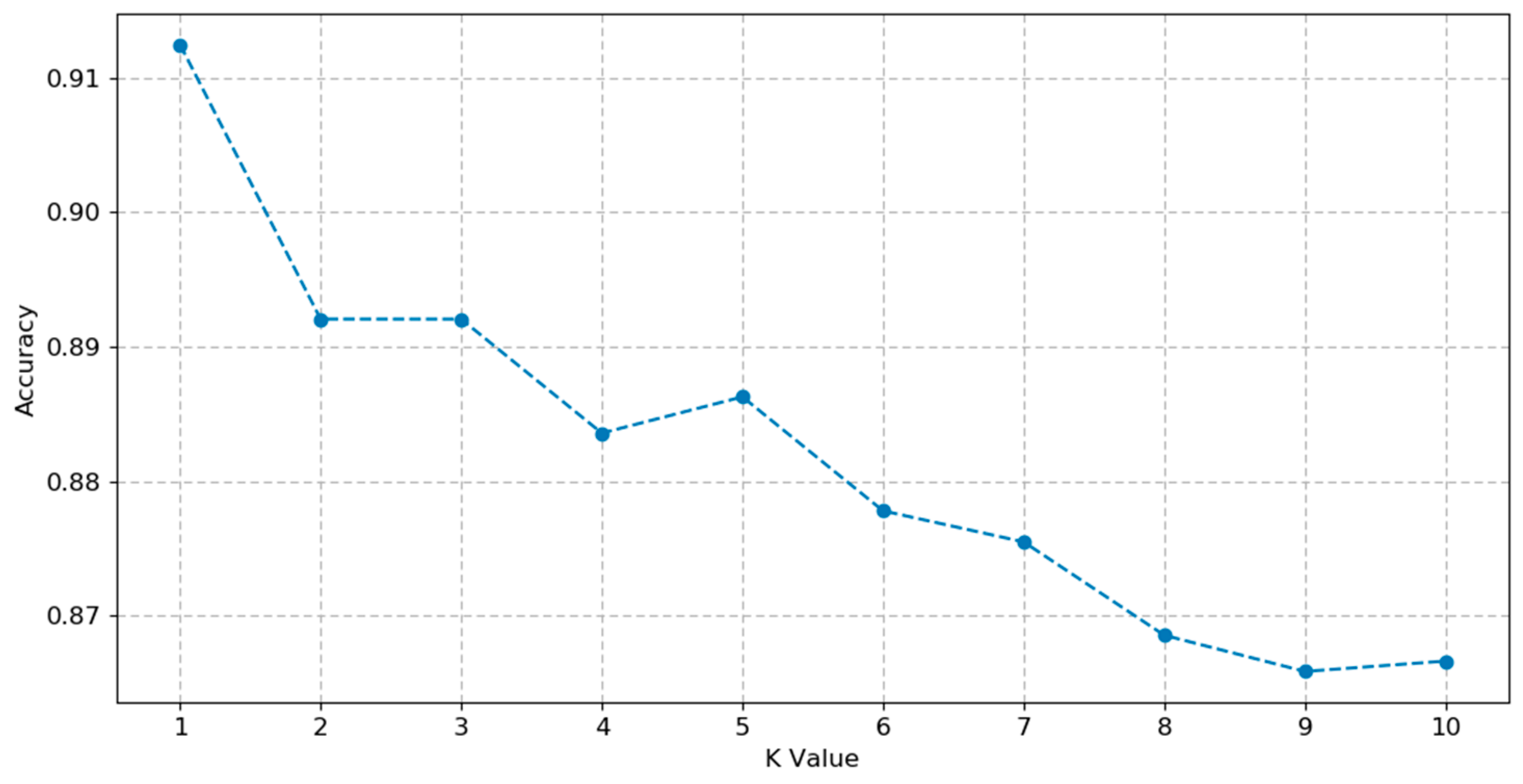
where P(t,N) is the simulated pressure for a specific time step t at a specific node N. is the mean pressure value for time step t and at node N for all samples. is the standard deviation of pressure suitable for time step t and at node N. To train the K-NN algorithm, 5-fold cross-validation was conducted. K was in the range of 1 to 10 and evaluated with accuracy parameter defined as the rate of correct predictions out of total prediction (Equation (7)):
The mean accuracy of the 5-fold cross-validation splits was calculated as shown in Figure 2. In most cases, K = 1 indicated overfitting of the model. This may have been due to an overly small database with a low variance between samples. In this case, increasing K would result in a more complex prediction model and increase the prediction bias. When testing the method on a “noised” database, the bias was significantly increased, and the best K was larger than 1.
3. Results
3.1. Tnet1 Network
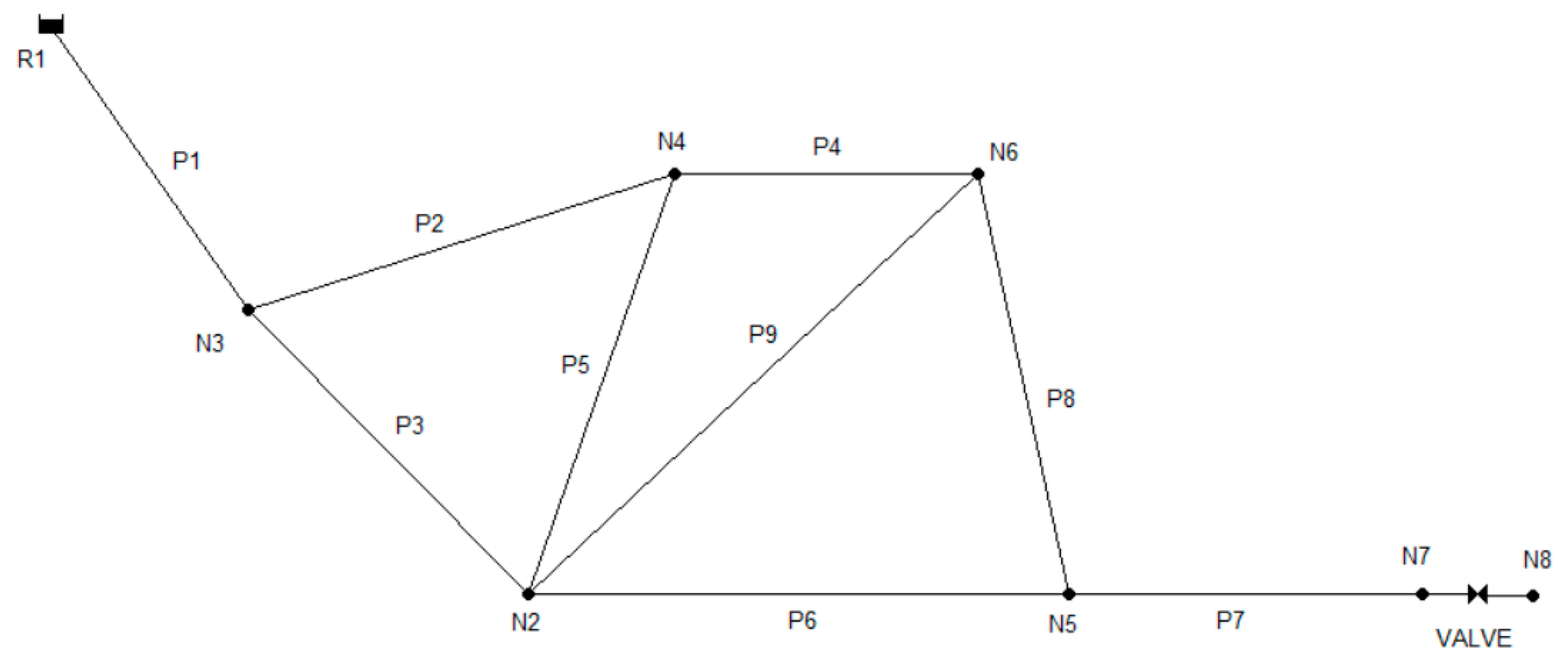
To explore the transient model’s ability to detect leaks in a water network, we started by applying this method to a relatively small network (nine pipes and six operative nodes). Figure 3 presents the Tnet1 layout.
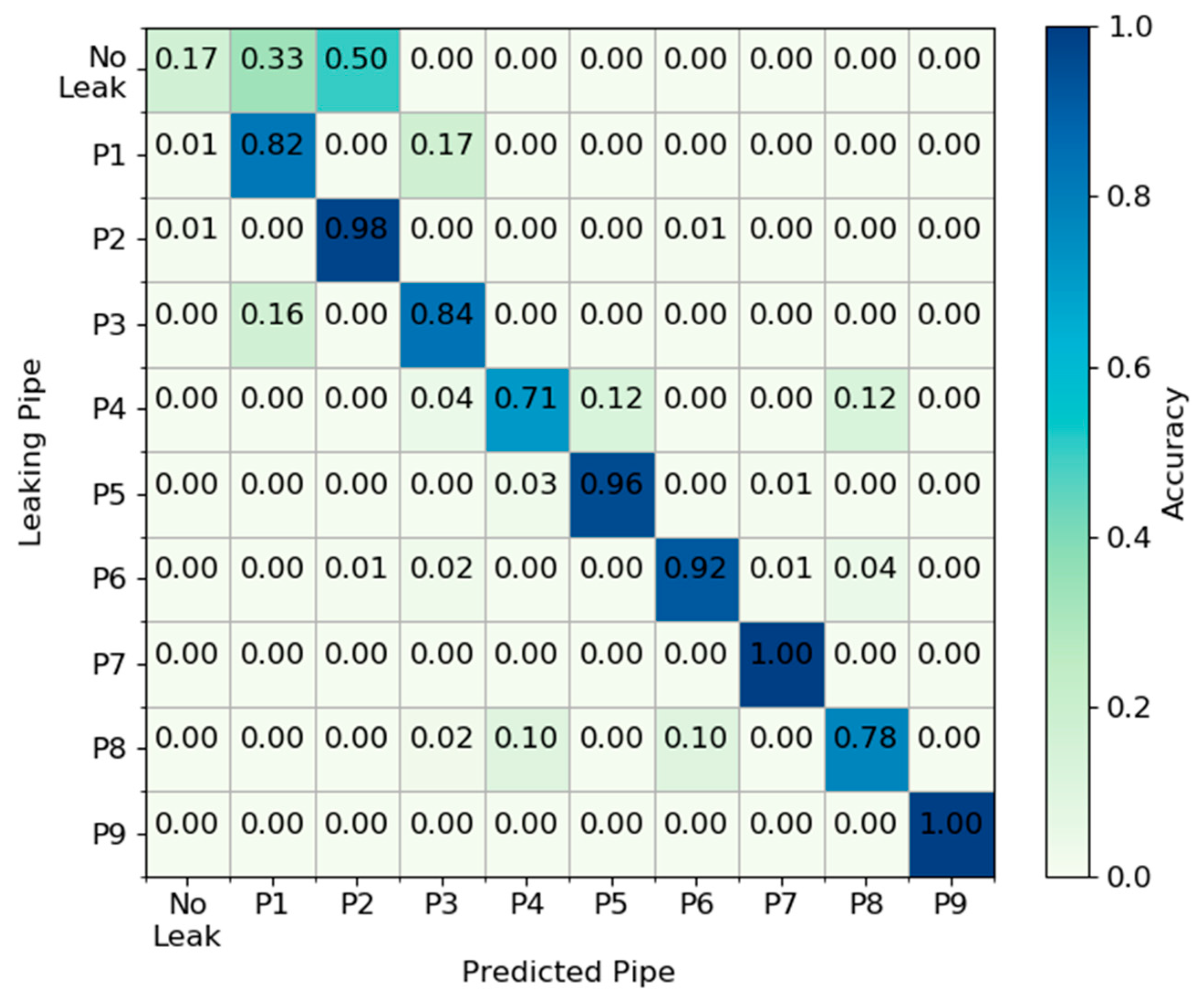
When generating the database, we defined the distance between the leak locations to be 100 m, with a leak size in the range of 0 to 15 mm with a 1 mm difference and six demand load configurations. The sampling pressure resolution was 25 Hz, and the simulation duration was 300 s, with pressure sensors in every node of the network except N8. The database was composed of 3706 samples and 7500 features. Although this is definitely a small database for learning algorithms, it was suitable as a proof of concept for the suggested methodology, which should yield better results with larger datasets. The first step was to train the K-NN model using 70% of the generated data and validate it using the other 30%. The result of this validation is presented in Figure 4. The overall accuracy of the validation set was 0.9. The model classified some pipes more accurately than others and failed to classify the ‘No leakage’ samples. To evaluate the model’s performance for every individual class (pipe), the Precision and Recall metrics were calculated. Precision states the number of actual leaking pipes among those that predicted as such (Equation (8)). Recall states for true positive rate meaning the rate of correctly predicted as leaking pipes out of the total number of leaking pipes (Equation (9)). Another metric calculated was F1, which states the harmonic average between Precision and Recall (Equation (10)). Table 2 illustrates a very strong correlation between the three parameters.
where TP is the number of true positive predictions (leaking and predicted as leaking pipe), FP is the number of false positive predictions (not leaking but predicted as leaking pipe), FN is the number of false negative predictions (does leaks but predicted as not leaking).
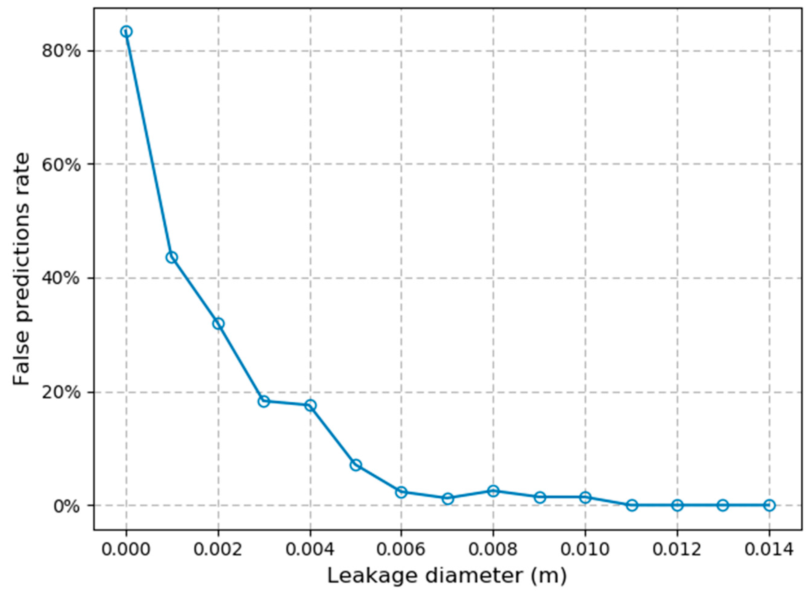
Figure 5 shows the dependence of the false prediction rate on the leak diameter, except for the ‘No leaks’ scenarios. This figure suggests that accurate prediction was more likely as the leak diameter increases. This result makes sense since bigger leaks will have a greater impact on network pressure.
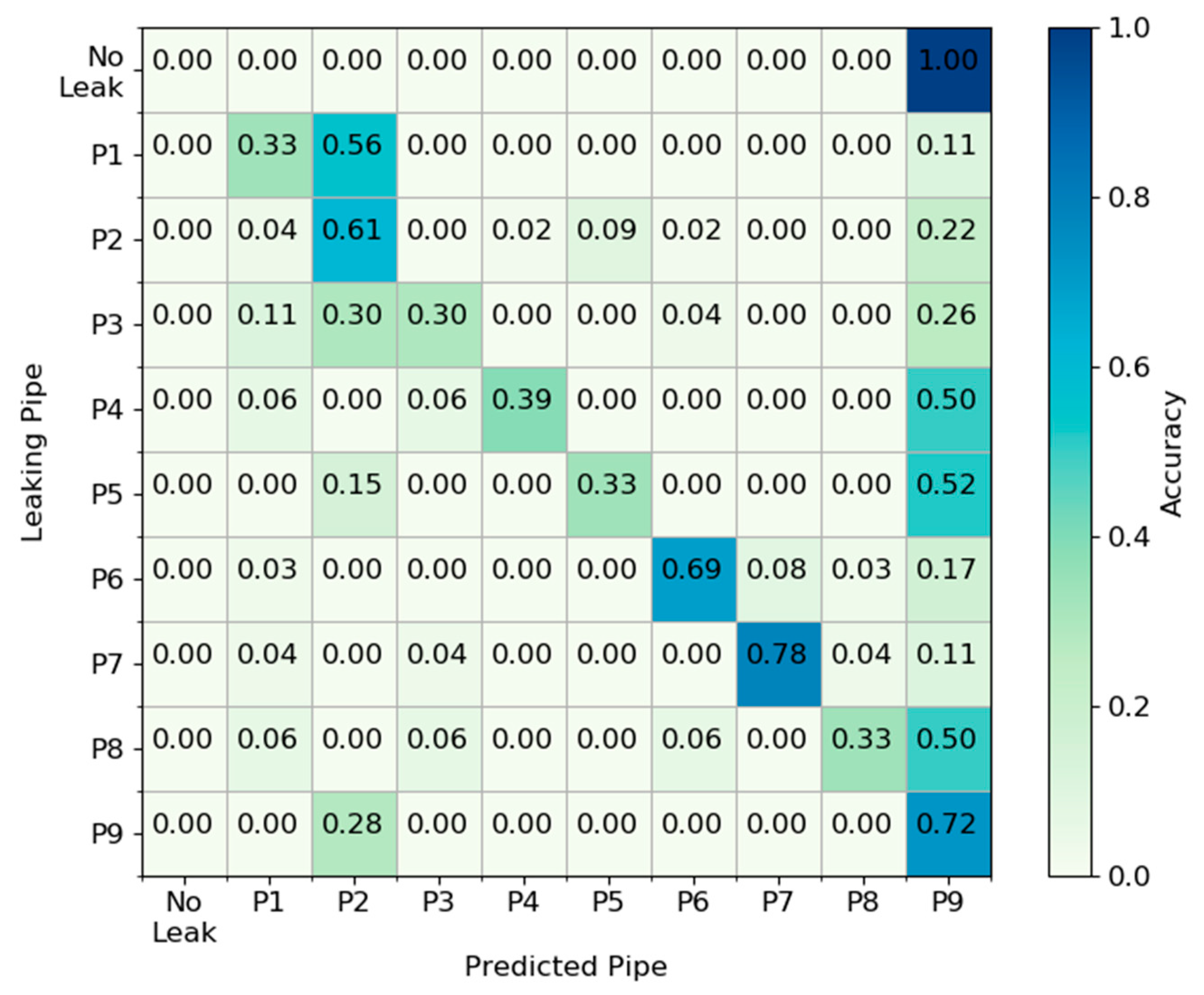
The next step was to test the trained K-NN algorithm using yet another database with one load configuration (different from the other six), where the distance between the leaks was 175 m, which located the leaks in places the algorithm had not seen before. The leak diameters were 1.5–15 mm with a 1.5 mm difference (diameters the algorithm had not seen before). The results of this test are presented in Figure 6, where the overall observed accuracy was 0.52. Although the accuracy was lower compared to the validation set, most of the false predictions occurred when the model predicted that the leakage was at pipe P9. This means that in these cases, further examination could have improved these results significantly.
3.2. Sensitivity Analysis
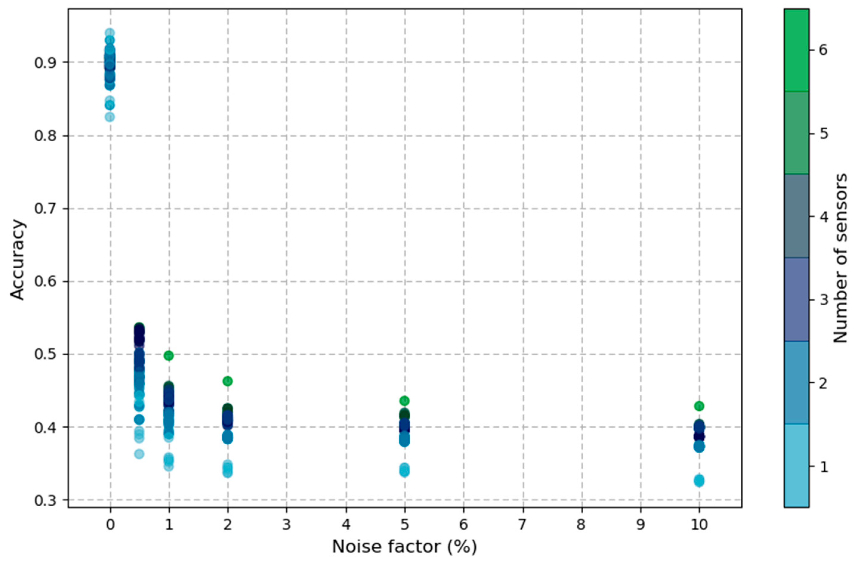
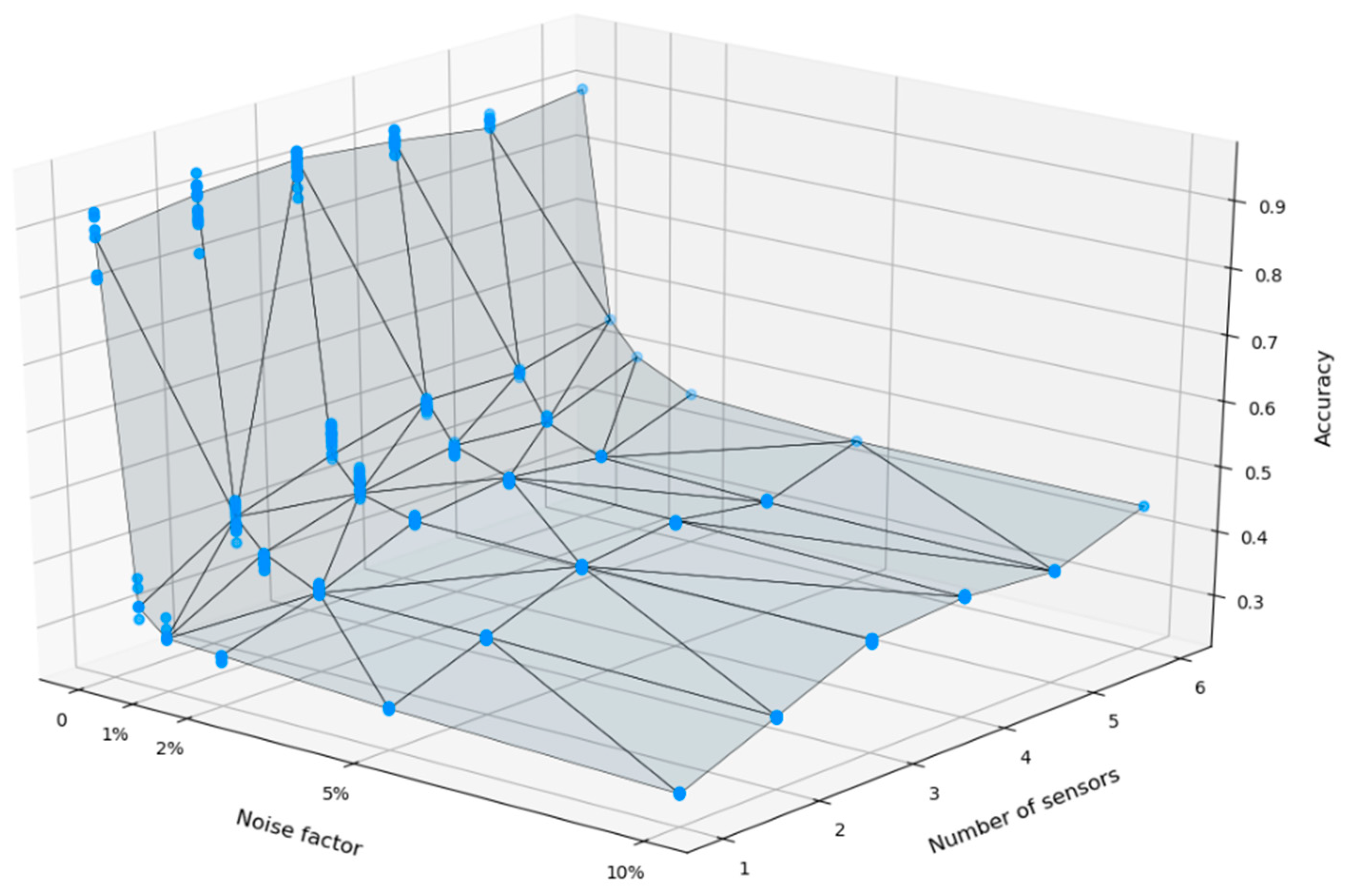
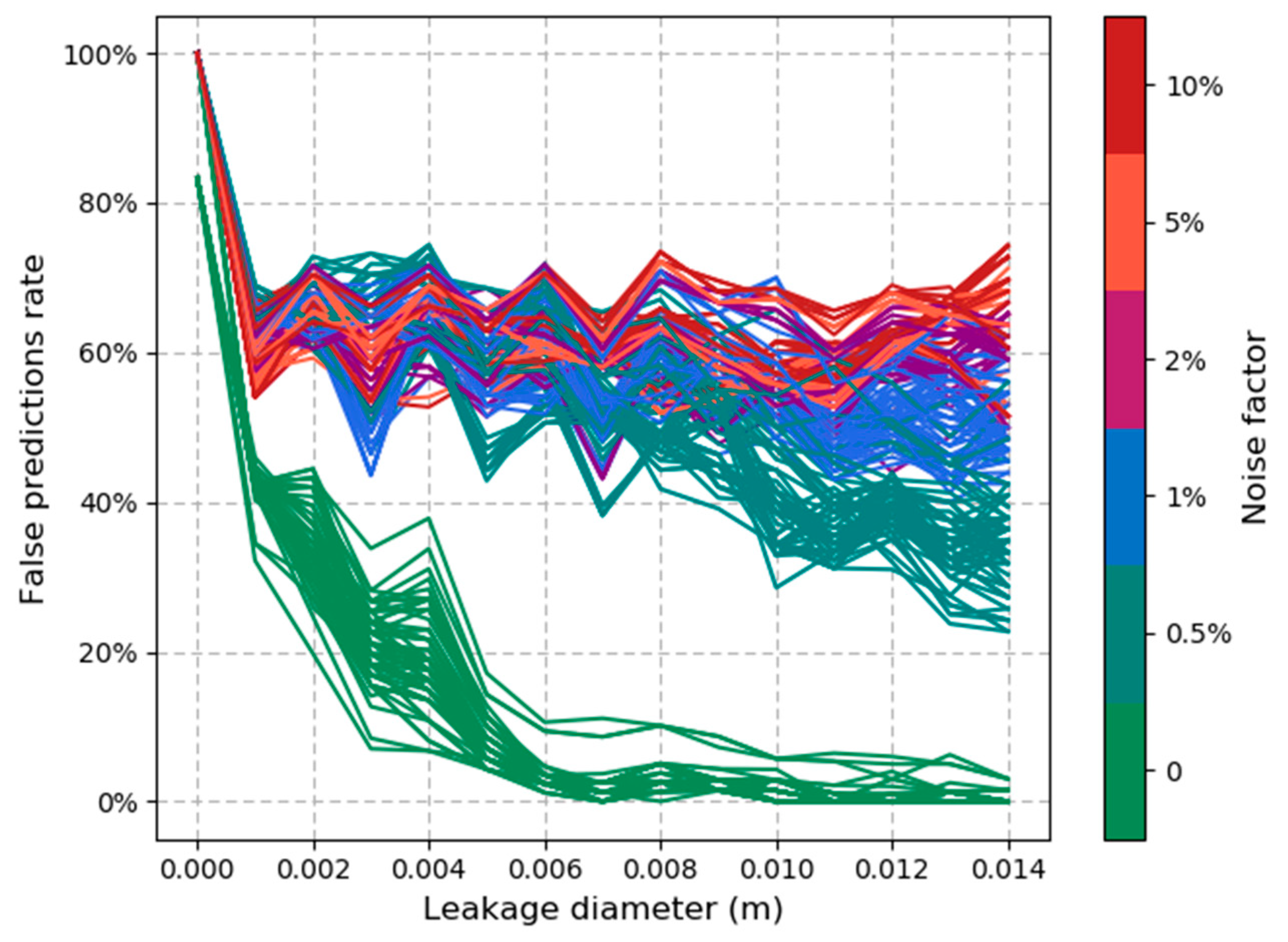
Figure 7 and Figure 8 present a sensitivity analysis for the methodology. They confirm that accuracy depended on the noise factor applied and the number of pressure sensors installed in the water network. Figure 7 shows that, as expected, with an increase in the noise factor, the ability to predict the leak location decreased accurately. As the noise factor increased, accurate prediction depended, to a greater extent, on the number of sensors installed. Even for a relatively small noise factor, the ability to accurately predict the leak location was affected considerably. This figure also presents the slight effect of enlarging the noise factor from 1 to 10%.
Another analysis was designed to identify the crucial factors responsible for accurate predictions. Figure 9 presents the Recall values for all the noise and sensor combination scenarios and shows the clear-cut influence of noised pressure values and leak diameters. This suggests that the methodology is highly sensitive to noising pressure values. Even a small factor of 0.5% impacted the prediction accuracy dramatically, as illustrated in Figure 9.
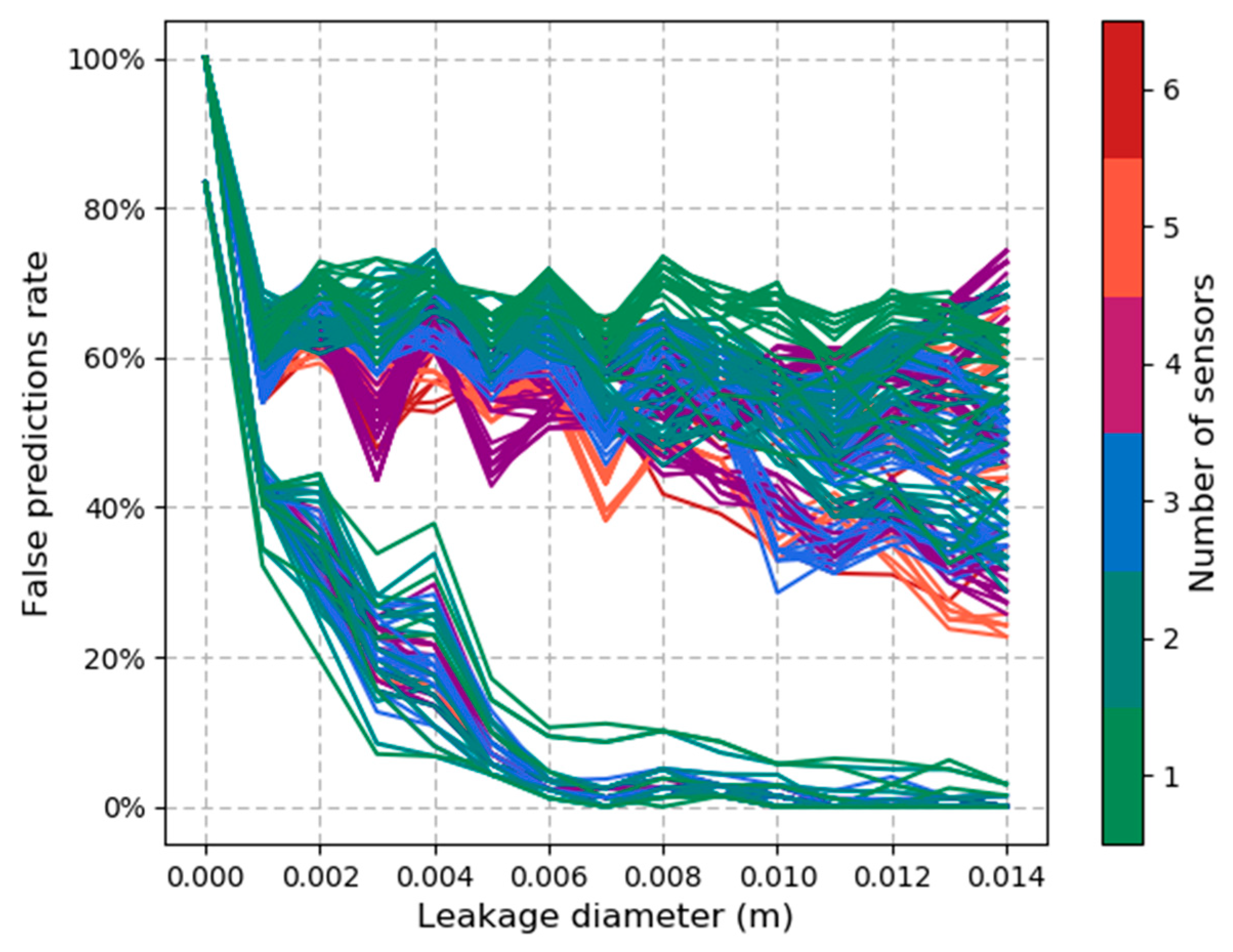
Similarly, another analysis investigated the influence of the network sensors. An examination of all the sensor combinations failed to identify one sensor that was more dominant than the others. Unexpectedly, Figure 10 shows that more sensors did not necessarily mean greater accuracy. In some cases, scenarios with the same noise factor achieved better results with three or four sensors than those with five or six sensors, as can be seen in Figure 10.
4. Conclusions and Research Opportunities
Water leakage is one of the acutest problems for water utilities. It causes water and energy loss as well as damage to other infrastructure and raises the risk for water contamination. As most pipes are buried underground, locating bursts is a challenging task. This study proposed a method that enables the prediction of whether a single pipe is leaking or not. The method based on advanced transient modeling generates a database describing the network’s response to varied leak scenarios. A new leak scenario can be classified according to the generated database using the K-NN algorithm. The model was tested on a small network and achieved satisfying results. In the current study, although the high-resolution pressures database was generated successfully, it was costly in terms of computer resources and its uncontrolled data size. The use of TSnet forced us to run the simulations with a time step that was smaller than desired. This small-time step required a heavier computing process and yielded overly detailed pressure head data. While diluting the database is possible, this would not reduce the burden of the computing process. On the other hand, once the database has been generated, the detection part can be executed immediately. Due to this limitation of computation resources, the method was tested only on a small network, and this is indeed the major limitation of the method, opening the door to a future research challenge to enable modeling a transient scenario in large networks and in a reasonable time. This will allow the generation of transient databases, which will open a wide range of methods that can analyze this data.
The second part classified measured pressure data to leakage events and showed good results, demonstrating the capabilities of this method. In a simple scenario, when the pressures in the network were not noised, an accuracy of 0.9 was obtained. However, the outcome was considerably degraded after we noised the data. Although this degraded, it was still capable of accurately predicting the leaking pipes in most cases. Attempting to classify interpolated data derived from the same water network but under consumption load we had not added to the generated database, the algorithm’s performance declined and only managed to classify some cases. The algorithm showed poor differentiation when the consumption load was an interpolation of the K-NN training data. When the consumption load was an extrapolation of the K-NN training data, the algorithm did not manage to predict the leaking pipes at all. Overall, the algorithm achieved a good result on a simple example but struggled as the problem complexity increased. Therefore, further research can analyze high-resolution noised pressure data to improve classification accuracy. This might be done with other, more sophisticated classification algorithms. Despite the limitations, it seems that transient modeling has the potential to uncover some hydraulic patterns not recognizable in regular hydraulic simulation. This type of modeling depends on larger data sets and requires computational power larger than other methods used in the past. With the growth in computer abilities, the authors expect that the suggested approach will be useful in the near future.
Author Contributions
Conceptualization and methodology, D.L. and G.P., supervision, A.O. All authors have read and agreed to the published version of the manuscript.
Funding
This research was funded by the Israel Science Foundation (grant No. 555/18).
Data Availability Statement
The data presented in this study are available on request from the corresponding author.
Conflicts of Interest
The authors declare no conflict of interest.
References
- Stephens, M.; Gong, J.; Zhang, C.; Marchi, A.; Dix, L.; Lambert, M.F. Leak-Before-Break Main Failure Prevention for Water Distribution Pipes Using Acoustic Smart Water Technologies: Case Study in Adelaide. J. Water Resour. 2020, 146, 05020020. [Google Scholar] [CrossRef]
- Cody, R.A.; Tolson, B.A.; Orchard, J. Detecting Leaks in Water Distribution Pipes Using a Deep Autoencoder and Hydroacoustic Spectrograms. J. Comput. Civ. Eng. 2020, 34, 04020001. [Google Scholar] [CrossRef]
- Choi, J.; Shin, J.; Song, C.; Han, S.; Park, D.I. Leak detection and location of water pipes using vibration sensors and modified ML prefilter. Sensors 2017, 17, 2104. [Google Scholar] [CrossRef] [PubMed] [Green Version]
- Gao, Y.; Brennan, M.J.; Joseph, P.F.; Muggleton, J.M.; Hunaidi, O. A model of the correlation function of leak noise in buried plastic pipes. J. Sound Vib. 2004, 277, 133–148. [Google Scholar] [CrossRef]
- Pérez, R.; Puig, V.; Pascual, J.; Peralta, A.; Landeros, E.; Jordanas, L. Pressure sensor distribution for leak detection in Barcelona water distribution network. Water Sci. Technol. Water Supply 2009, 9, 715–721. [Google Scholar] [CrossRef]
- Rocher, J.; Parra, L.; Lloret, J.; Mengual, J. An Unductive Sensor for Water Level Monitoring in Tubes for Water Grids. In Proceedings of the 2018 IEEE/ACS 15th International Conference on Computer Systems and Applications, Aqaba, Jordan, 28 October–1 November 2018. [Google Scholar]
- Zhang, X.; Yu, M.; Ma, Z.; Ouyang, H.; Zou, Y.; Zhang, S.L.; Niu, H.; Pan, X.; Xu, M.; Li, Z.; et al. Self-Powered Distributed Water Level Sensors Based on Liquid–Solid Triboelectric Nanogenerators for Ship Draft Detecting. Adv. Funct. Mater. 2019, 29, 1900327. [Google Scholar] [CrossRef]
- Wang, Z.; Song, H.; Watkins, D.W.; Ong, K.G.; Xue, P.; Yang, Q.; Shi, X. Cyber-Physical Systems for Water Sustainability: Challenges and Opportunities. IEEE Commun. Mag. 2015, 53, 216–222. [Google Scholar] [CrossRef] [Green Version]
- Kühnert, C.; Bernard, T.; Montalvo Arango, I.; Nitsche, R. Water quality supervision of distribution networks based on machine learning algorithms and operator feedback. Procedia Eng. 2014, 89, 189–196. [Google Scholar] [CrossRef]
- Aminravan, F.; Sadiq, R.; Hoorfar, M.; Rodriguez, M.J.; Najjaran, H. Multi-level information fusion for spatiotemporal monitoring in water distribution networks. Expert Syst. Appl. 2015, 42, 3813–3831. [Google Scholar] [CrossRef]
- Stephens, M.; Gong, J.; Marchi, A.; Dix, L.; Lambert, M. Field Testing of Adelaide CBD Smart Network Acoustic Technologies. In Proceedings of the 1st International WSDA/CCWI 2018 Joint Conference, Kingston, ON, Canada, 23–25 July 2018. [Google Scholar]
- Steffelbauer, D.B.; Deuerlein, J.; Gilbert, D.; Piller, O.; Abraham, E. A Dual Model For Leak Detection and Localization: BattLeDIM 2020-Battle of the Leakage Detection and Isolation Methods Team: Under Pressure. In Proceedings of the 2nd International CCWI / WDSA, Beijing, China, 30 June 2020. [Google Scholar] [CrossRef]
- Li, Z.; Xin, K. Fast Localization of Multiple Leaks in Water Distribution Network Jointly Driven By Simulation and Machine Learning. Zenodo 2020. [Google Scholar] [CrossRef]
- Izquierdo, J.; López, P.A.; Martínez, F.J.; Pérez, R. Fault detection in water supply systems using hybrid (theory and data-driven) modelling. Math. Comput. Model. 2007, 46, 341–350. [Google Scholar] [CrossRef]
- Zhang, Q.; Wu, Z.Y.; Zhao, M.; Qi, J.; Huang, Y.; Zhao, H. Leakage Zone Identification in Large-Scale Water Distribution Systems Using Multiclass Support Vector Machines. J. Water Resour. 2016, 142, 04016042. [Google Scholar] [CrossRef]
- Fang, Q.S.; Zhang, J.X.; Xie, C.L.; Yang, Y.L. Detection of multiple leakage points in water distribution networks based on convolutional neural networks. Water Sci. Technol. Water Supply 2019, 19, 2231–2239. [Google Scholar] [CrossRef]
- Xing, L.; Sela, L. Transient simulations in water distribution networks: TSNet python package. Adv. Eng. Softw. 2020, 149, 102884. [Google Scholar] [CrossRef]
- Xing, L.; Sela, L. TSNet Documentation Release 0.2.0. Available online: https://www.researchgate.net/publication/341434146 (accessed on 23 February 2021).
- Klise, K.; Hart, D.; Moriarty, D.; Bynum, M.; Murray, R. Water Network Tool for Resilience (WNTR) User Manual, 2017, United States Environmental Protection Agency Office of Research and Development, Washington, DC, USA. Available online: https://cfpub.epa.gov/si/si_public_record_report.cfm?dirEntryId=337888&Lab=NRMRL (accessed on 23 February 2021).
- Crowl, D.A.; Louvar, J.F. Chemical Process Safety—Fundamentals with Applications, 2nd ed.; Prentice Hall PTR: Upper Saddle River, NJ, USA, 2019; pp. 112–116. ISBN 10:0130181765. [Google Scholar]
- Cover, T.M.; Hart, P.E. Nearest neighbor pattern classification. IEEE Trans. Inf. Theory 1967, 13, 21–27. [Google Scholar] [CrossRef]
Figure 1.
Two leaks located on the same pipe as seen from a neighbor node.

Figure 2.
Mean accuracy as a function of K.

Figure 3.
Tnet1 network layout.

Figure 4.
Tnet1 K-nearest neighbor (K-NN) algorithm first validation.

Figure 5.
Tnet1 false predictions as a function of leak diameter.

Figure 6.
Tnet1 K-NN second validation.

Figure 7.
Tnet1 accurate leak location prediction as a function of the noise factor and the number of sensors.
Figure 7.
Tnet1 accurate leak location prediction as a function of the noise factor and the number of sensors.

Figure 8.
Tnet1 accurate leak location prediction as a function of the noise factor and the number of sensors—3D.
Figure 8.
Tnet1 accurate leak location prediction as a function of the noise factor and the number of sensors—3D.

Figure 9.
The impact of the noise factor on the prediction accuracy.

Figure 10.
The impact of the number of sensors on prediction accuracy.


Table 1.
The structure of the database.
| N1, t1 | N1, t2 | … | N2, t1 | N2, t2 | … | Nn, t1 | Nn, T | Pipe | Distance | Diameter |
|---|---|---|---|---|---|---|---|---|---|---|
| 190.99 | 190.99 | 190.98 | 190.98 | 190.97 | 190.97 | P6 | 500 | 0.004 | ||
| ⋮ | ⋮ | ⋮ | ⋮ | ⋮ | ⋮ | ⋮ | ⋮ | ⋮ | ⋮ | ⋮ |
Table 2.
Leaking pipe prediction parameters.
| Pipe ID | Precision | Recall | F1-Score | Support |
|---|---|---|---|---|
| No Leakage | 0.25 | 0.17 | 0.2 | 6 |
| 1 | 0.83 | 0.82 | 0.82 | 128 |
| 2 | 0.98 | 0.98 | 0.98 | 195 |
| 3 | 0.78 | 0.84 | 0.81 | 124 |
| 4 | 0.81 | 0.71 | 0.76 | 73 |
| 5 | 0.92 | 0.96 | 0.94 | 101 |
| 6 | 0.91 | 0.92 | 0.92 | 127 |
| 7 | 0.99 | 1 | 0.99 | 196 |
| 8 | 0.83 | 0.78 | 0.8 | 89 |
| 9 | 1 | 1 | 1 | 73 |
| accuracy | 0.9 | 1112 | ||
| macro avg. | 0.83 | 0.82 | 0.82 | 1112 |
| weighted avg. | 0.9 | 0.9 | 0.9 | 1112 |
Publisher’s Note: MDPI stays neutral with regard to jurisdictional claims in published maps and institutional affiliations. |
© 2021 by the authors. Licensee MDPI, Basel, Switzerland. This article is an open access article distributed under the terms and conditions of the Creative Commons Attribution (CC BY) license (http://creativecommons.org/licenses/by/4.0/).
Share and Cite
MDPI and ACS Style
Levinas, D.; Perelman, G.; Ostfeld, A. Water Leak Localization Using High-Resolution Pressure Sensors. Water 2021, 13, 591. https://doi.org/10.3390/w13050591
AMA Style
Levinas D, Perelman G, Ostfeld A. Water Leak Localization Using High-Resolution Pressure Sensors. Water. 2021; 13(5):591. https://doi.org/10.3390/w13050591
Chicago/Turabian StyleLevinas, Daniel, Gal Perelman, and Avi Ostfeld. 2021. "Water Leak Localization Using High-Resolution Pressure Sensors" Water 13, no. 5: 591. https://doi.org/10.3390/w13050591
Note that from the first issue of 2016, this journal uses article numbers instead of page numbers. See further details here.