Study of the Wet Bulb in Stratified Soils (Sand-Covered Soil) in Intensive Greenhouse Agriculture under Drip Irrigation by Calibrating the Hydrus-3D Model

Abstract

The development of the wet bulb under drip irrigation in sand-covered soils presents a different behavior compared to the one observed in homogeneous soils. Moreover, the presence of a very active crop imposes a series of variations that have not been fully characterized. The aim of this work is to present the data acquisition methodology to calibrate and validate the Hydrus-3D model in order to safely define the evolution of moisture in wet bulbs generated in stratified “sanded” soils characteristic of greenhouses with intensive pepper crop under drip irrigation. The procedure for collecting and processing moisture data in stratified soils has been defined. Soil permeability; retention curve, texture, and bulk density have been measured experimentally for each material. It has been found that the inclusion of a previous day in the simulation improves model predictions of soil moisture distribution. In soils with less gravel, a lower average stress and a more homogeneous moisture distribution were observed. It has been proved that the Hydrus-3D model can reproduce the behavior of sand covered soils under intensive greenhouse growing conditions, and it has been possible to verify that the predictions are adequate to what has been observed in the field. In view of the results, the Hydrus-3D model could be used to establish future irrigation strategies or to locate the optimal placement point of tensiometers that control irrigation in sandy soils for intensive agriculture.

1. Introduction

Greenhouse cultivation has proven to be an energy [1] and water [2] efficient solution for extra-early vegetable production, which allows maintaining the vegetable production cycle throughout the year. This production depends on many factors, perhaps the main one being the localized irrigation system. In this area, the availability and quality of irrigation water will be one of the most limiting factors for the development of this agricultural practice.

The use of sand covers to improve soil moisture and temperature has been known for a long time [3,4]. In the intensive crops of the Spanish Southeast, it began to be used from the middle of the 20th century, fundamentally to avoid evaporation from the soil [5] and the capillary rise of the salts contained in the water available for irrigation [6]. This fact, together with the poor quality of the available soils and the presence of more or less large pieces of limestone at the base of these, frequently appearing in extensive areas, made the farmer seek to improve it with the contribution of fertile soil from other areas.

Fortunately, in the zone there are lacustrine deposits of clayey materials that were used almost immediately for this purpose. A thin layer of organic matter (manure, compost, or peat) was added to the layer of more or less clayey soil and the layer of sand to improve the root environment. Sandblasting, as it has become standardized today, is a technique that consists of placing a layer of soil between 0.15 and 0.40 m above the original material, a thin layer (0.005 to 0.010 m) of organic matter, and on top of this a layer of sand of about 0.05 to 0.10 m. An outline of this arrangement is shown in Figure 1.

For the correct design and management of localized irrigation systems, it is necessary to know the shape of the wet bulb formed by the emitters [7]. Flow from a drip emitter, due to its multi-dimensional nature and high frequency of water application, entails a certain complexity of soil moisture modeling dynamics [8]. Therefore, numerous authors have attempted to define the evolution of the wet bulb in drip irrigation using macroscopic models. For example, Schwartzman and Zur [9] developed an empirical model to estimate the vertical and horizontal distances of a wetting front from a surface point source. Amin and Ekhmaj [10] verified this model using several experimental data sets and modified it by including saturated soil water content as one of the model parameters. Finally, Kandelous et al. [11] developed an empirical model to estimate the upward, downward, and horizontal distances of the wetting front from a subsurface point source. There have also been attempts to approach the problem from a more rational point of view [12,13].

In stratified soils, such as “sanded” soils, water distribution can change substantially with respect to the case of homogeneous soils [14]. The characteristics of the base layer and sand cover have a great influence [15], as it does not allow a clear view of the wet or dry area and may also favor the circulation of water through preferential routes. In addition, it is possible that the wet bulbs overlap in a relatively short time since the usual practice is to separate the emitters a very small distance, typically 0.2 to 0.5 m [16].

The influence of the root is also not negligible, since the consumption must be attended from a relatively small volume of soil so that the drying of the profile can be quite fast [17]. Different measurement techniques have been used to visualize the role of the root in the wet bulbs formation of in this type of soil, from direct measurements in soil profile cuts [18] to the direct monitoring of root distribution [19] or different soil parameters such as water tension in the soil or moisture content [20].

The Hydrus Model, originally proposed by Šimunek et al. [21] can be used both for direct problems when the initial and boundary conditions of all processes involved and for the corresponding model parameters are known, and for inverse problems when some of the parameters must be calibrated or estimated from observed data. The movement of water in the soil, in this model, is based on the numerical resolution of the Richards’ equation [22].

This model has been widely used to simulate water flow and solute transport in soils and groundwater with varying saturation [23,24]. Surface [25] and sprinkler irrigation [26] processes have also been successfully simulated with this tool. However, where this model reaches one of its greatest potential is in the study of localized irrigation [27,28] in its 2D and 3D versions. Elnesr and Alazba [29] showed that 3D simulations are more successful and reliable than 2D simulations in terms of mass balance error.

Several authors [30], using tensiometers and neutron probe, have addressed the parameterization of this model and they found that the fit of the simulations was better at positions close to the dripper and worse at positions outside its wetting pattern. Even the overlap between wet bulbs has been studied with this model [31] and simulations of the water content and wetting front were close to the observed data.

However, although there are studies on the application of Hydrus on stratified soils [32,33,34], in general, they refer to vertical infiltration processes and there are few works on the application of Hydrus 3D on moisture movement processes in three dimensions in stratified soils [35,36]. It is important to note, however, that this type of soil requires careful analysis since it is made up of layers of different origins, with a very homogeneous texture in each layer but is very different between them, which would never be found arranged in such a pattern in natural soils. Furthermore, Hydrus has not been applied or, consequently, calibrated in this type of soils typical of these greenhouses with intensive production.

Proposing solutions for this kind of soils is of enormous scientific and economic interest since crops managed in this way are estimated to provide fresh vegetables to 56 million people in Europe during the winter [37]. The aim of this work is to present the methodology of data acquisition and the actions carried out to properly calibrate the Hydrus-3D model in order to safely define the evolution of moisture in wet bulbs generated in stratified “sanded” soils used in intensive horticultural greenhouse crops under the usual irrigation conditions in this area.

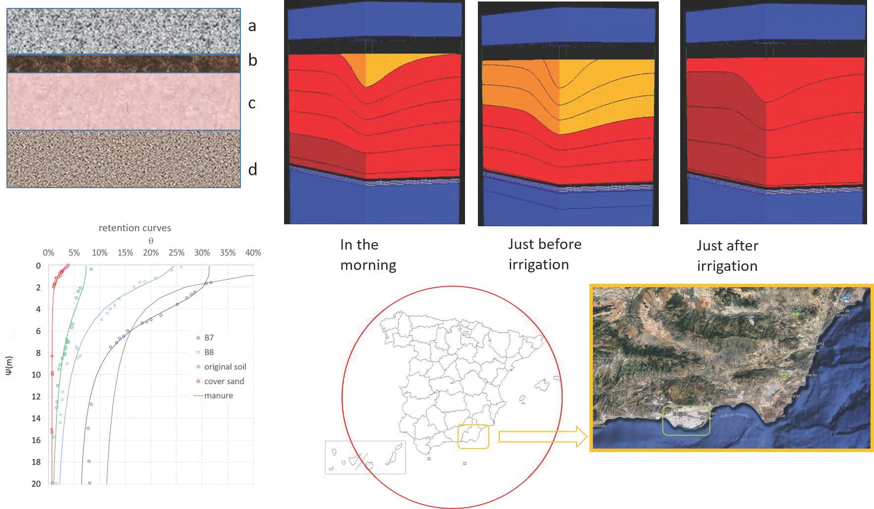
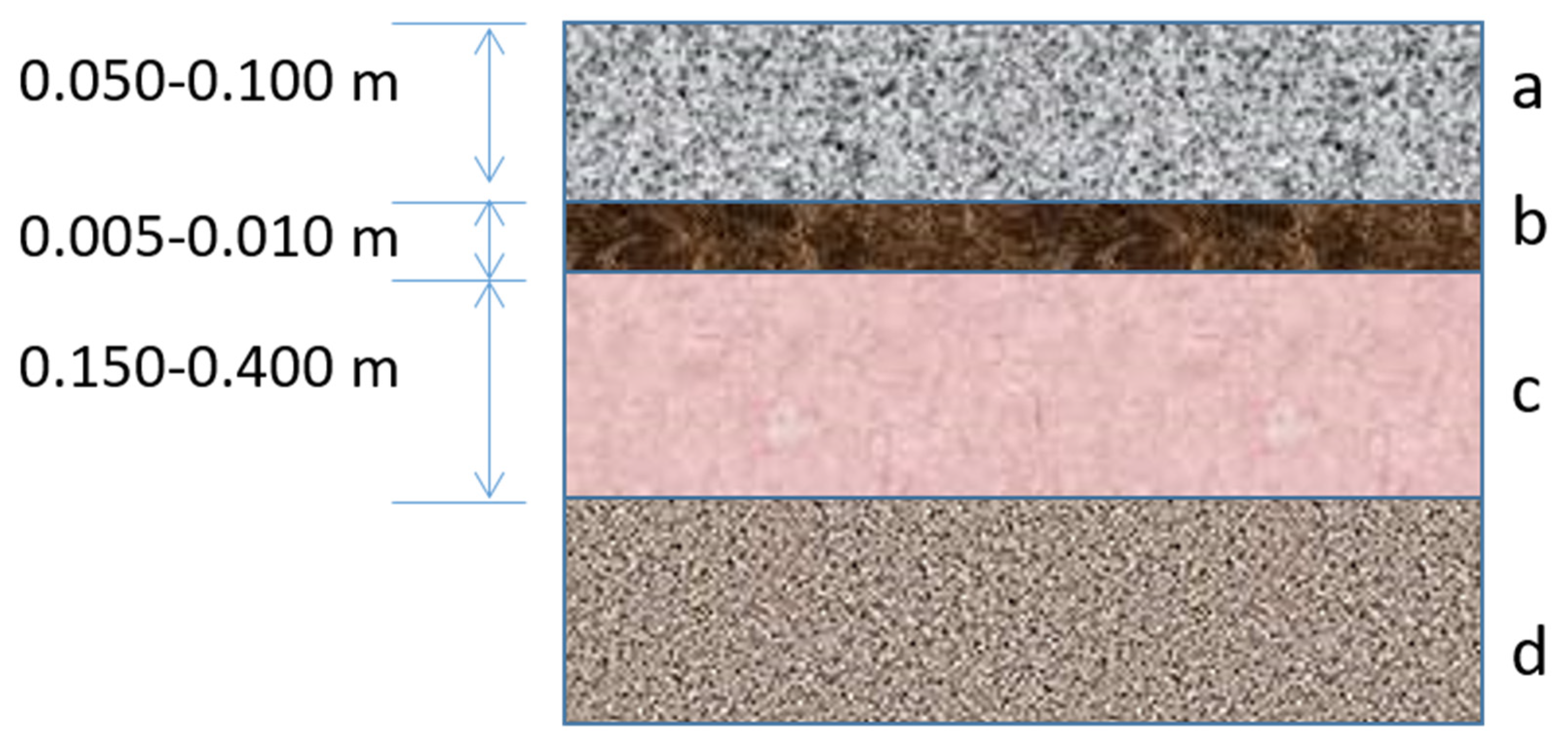
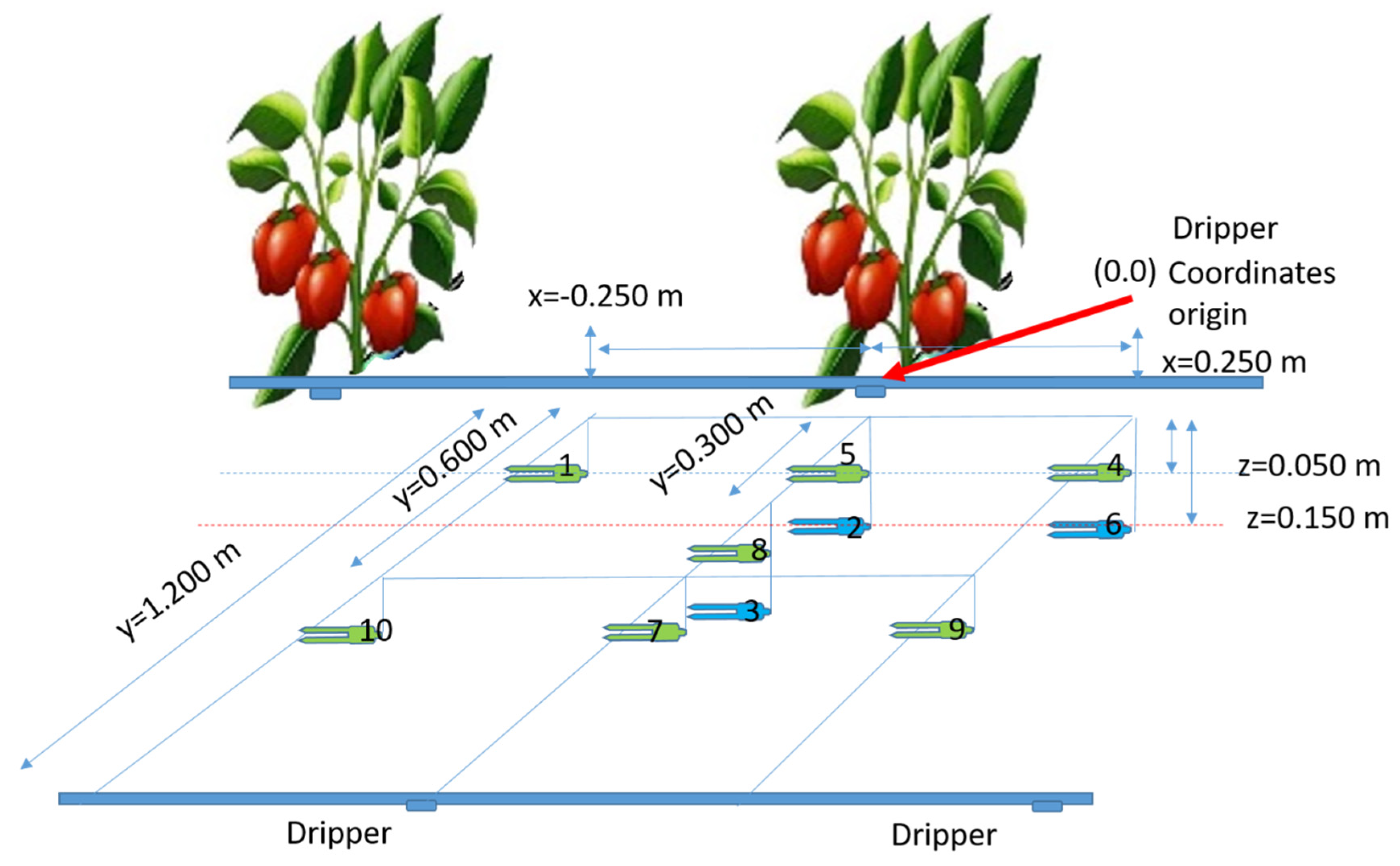
2. Materials and Methods

Test location

The trials were carried out at the IFAPA Center La Mojonera (Almeria, Spain). For the experimentation, two multi-tunnel type greenhouses of 900 m² called B7 and B8 were used. The position of the center as well as the precise location of the tests are shown in Figure 2.

Watering system

The watering system is automatic, with drippers of nominal flow Qn = 8.33 × 10⁻⁷ m³·s⁻¹, self-compensating, and Netafim PJC Anti-drainage. The irrigation pipes are arranged in paired lanes, with a distance between them of 0.65 m and a distance between lanes of 1.20 m. Within the watering line, the emitters are spaced by 0.5 m apart. The arrangement of the watering frame is shown in Figure 3. Irrigation control is carried out by means of classic tensiometers with a built-in pressure transducer, which indicates to a computer that the set tension has been reached and this commands the irrigation automaton to carry it out by automatically opening and closing electrovalves. Following the usual recommendations for irrigation in the area, for sweet pepper, a tension of ψ = 1 m was set, the programmed irrigation time was of 1200 s. Under these conditions, humidity variations are expected to be minimal that will allow testing the sensitivity of the probes and the model.

Soil

The soil, in both greenhouses, is the typical layered soil used for horticultural crop in Almeria. The sand layer was 0.050 m, the organic layer 0.005 m, and the added soil layer 0.150 m. On the other hand, the added soil is different in both cases, and although both are of a clayey texture, B8 soil has 33% coarse materials (D > 0.002 m), and the one corresponding to greenhouse B7, only contains 3% coarse materials. The original material varied from sandy loam to clay loam as depth increased.

A vertical core was taken on each kind of soil and each sample was subdivided respecting the changes in material and in any case with a maximum thickness of 0.050 m. Each sample was dried in the laboratory and each subsample was analyzed separately. The gravel and coarse sand were separated by sieving at 0.002 m and 0.0005 m, the rest, the fine fraction, was analyzed by the Bouyoucos densimeter technique [38] to obtain the different textural classes (clay, silt, and sand). The variation of each fraction obtained as a function of depth is shown in Figure 4.

From a textural point of view both soils are clayey in its contributed part and sandy loam in its basal part. This circumstance can lead to calculation errors since both are different in the distribution of the coarser elements. For this reason, it is necessary to measure the soil moisture retention curve.

The textures of the soils provided are representative of the horticultural crop of Almeria. The contributed soil with very few coarse elements, obtained by decanting clays from materials coming from quarries is called B7, and the soil with a clayey material coming directly from quarries and containing a considerable fraction of coarse materials is called B8. The original soil layer is highly permeable alluvial gravel. This soil allows the washing of salts, but requires a finer control of the irrigation water so that it is not lost excessively in the form of drainage.

In Figure 4 and Figure 5, the blue zone represents the original soil, the ochre zone represents the added soil, and the dark band represents the manure layer.

It has been observed that the bulk density took very high values, so a determination of this was made. The obtained values are shown in Figure 5.

In both cases, a high bulk density is observed for the clayey texture layer in the first centimeters, probably due to the passage of the people tending the crop and the compaction that the material suffers during its addition. This circumstance favors a more horizontal distribution of the roots since the penetration in depth is difficult. The original soil, on the other hand, presents normal characteristics for its texture.

Crop management

The crop was sweet pepper (Capsicum annuum L var. Mazo) planted on 17 September, 2018. The water was obtained from desalinated water and saline well water, which was mixed until the desired conductivity was achieved, in this case CEw = 1 dS·m⁻¹. In addition, an irrigation control was carried out by means of Irrometer-SR tensiometers, 30 cm in length with a coupled transducer that allows automating the irrigation. They were installed at 0.130 m from the irrigation line and at 0.130 m from the line perpendicular to the pipe, which crosses the plant’s stem. The installation depth was also, 0.130 m with respect to the level of the soil provided. In the study area, it is common to use this type of tensiometer, and in this specific case, the activation tension was 1 m. Once the watering was activated, the duration was fixed on 1200 s.

Moisture measurement

The control was carried out at two depths: Just under the sand layer (z = 0.100 m) and at the bottom of the crop profile (z = 0.200 m). In these facilities, a weather station records data of reference evapotranspiration inside an Almeria type greenhouse every hour to monitor the crop water extractions.

Moisture was measured at 10 points distributed around a dripper as indicated in Figure 3. Seven probes at 0.050 m depth in the added soil layer (z = 0.100 m) and three probes at a 0.150 m depth were placed near the original soil layer (z = 0.200 m). The sensor used is the so-called TE5 from Decagon Devices Inc. (Pullman Washington, DC, USA). The signal from each sensor was collected through a communication protocol that allows the sequential collection of a very high number of signals (more than 20 different ones), then scaled by a processor, and stored in a small internal memory. When the system detects that it has coverage, it is sent to the network where it is stored on the manufacturer’s website and from there it can be downloaded to the research team’s computers. The sampling frequency has been set at one piece of data every minute.

Installation of the equipment

The planting frame coincides with the drippers, being the separation between drippers, Sg = 0.500 m and the separation between irrigation pipes, Sr = 1.200 m, for this reason the probes were placed up to the middle of the planting frame. The coordinates of each probe were taken with respect to the dripper and the factory reference of each probe was noted to always check the consistency of the data series. In this first phase, it was considered that the soil was homogeneous in each layer and therefore a quadrant of the drip frame was checked

On 16 October 2018, the sensors were installed in the first test point, with B7 soil. Days later, on 26 October 2018, the second unit was also installed in the soil B8 and the arrangement of the probes was identical in each test and is shown in Figure 3, although the numbering has sometimes changed for reasons of equipment configuration. On the other hand, the exact positions of each probe are shown in

Table 1. Position of probes, considering the dripper as (0,0,0) coordinates, in sweet pepper (2018–19).

Equipment 1 Soil B7				Equipment 2 Soil B8
Probe	x (m)	y (m)	z (m)	Probe	x (m)	y (m)	z (m)
1	0.250	0	0.050	1	−0.250	0	0.050
2	−0.250	0	0.050	2	0	0	0.150
3	0	0.300	0.050	3	0	0.300	0.150
4	−0.250	0	0.150	4	0.250	0	0.050
5	−0.250	0	0.050	5	0	0	0.050
6	0.250	0	0.050	6	0.250	0	0.150
7	0	0	0.150	7	0	0.600	0.050
8	0	0	0.050	8	0	0.300	0.050
9	0	0.300	0.150	9	0.250	0.600	0.050
10	0	0.600	0.050	10	−0.250	0.600	0.050

. This distribution was considered adequate to have more information about the points, a priori more interesting, with the possibility of changing it if the results would make it advisable later. According to the manufacturer, the probes integrate measurements of a volume of about 250 cm³ and their influence extends about 3 cm around the probe. Therefore, they were installed horizontally in order to collect data from depths as close as possible.

Figure 6 shows a diagram of the arrangement of the probes on the ground B8 indicating the position of the probes in the two selected depths.

The equipment is removed for maintenance and recalibration in July, when the cultivation period ends, following the usual practice in the area.

Characterization of soil parameters for the Hydrus-3D model

The Hydrus-3D model, with which the data was processed, is demanding in terms of parameters. For a good result, it is necessary to characterize the texture, the distribution of roots, the retention curve, as well as the permeability of each proposed material.

The soil moisture retention curve is an interesting tool for agronomic management and is important in the characterization of water and salt movement in soils. This expression estimates the soil moisture retention as a function of humidity [39,40] and in our case the best adjustments were obtained with those proposed by Van Genuchten, as a function of moisture θ, residual moisture θr, porosity θs, inverse of air entry potential α, an exponent n, and the tension ψ.

In this work the retention curve used is (Equation (1)):

$$S=\frac{\theta -{\theta }_r}{{\theta }_s-{\theta }_r}={\left(1+{\left(\alpha \psi \right)}^n\right)}^{-\left(1-\frac{1}{n}\right)}$$

(1)

where the different coefficients can be obtained from texture data or from the curves measured directly from soil samples. In this case, it was decided to determine the curve directly and then adjust the parameters through an optimization scheme based on minimizing the sum of squared errors. The nonlinear Generalized Reduced Gradient GRG resolution method has been used.

Soil samples were taken from the greenhouses where the test was conducted. Soil samples were also taken from the base, which had a sandy texture and included gravel. Finally, a sample of the surface sand was taken. The samples were taken in 1-L cans, all of them equal, trying to keep the sample unaltered.

Moisture was measured by weighing the sample on consecutive days and drying it in an oven at the end of the series of measurements. For this reason, and so that the data was suitable for the Hydrus-3D model, the bulk density of the sample was also measured. The tension was measured with Irrometer Watermark plaster block tensiometers and the recording was made with the device offered by the manufacturer.

Samples and sensors were arranged on 11 December 2018 and data was recorded until 18 February 2019. The device was set up in a laboratory at room temperature and the measurements were all taken at 8:30 am. The units of measurement for humidity were those offered by the device (%) and the tension measurements were in the same way in cbar and then converted in m.

The hydraulic conductivity at saturation, ks, was determined by means of a vertical permeameter with a constant load under saturation conditions. The sample was taken by means of a cylinder tapered towards the interior and in this same device, the permeability was measured.

Root calibration for Hydrus-3D model

The root distribution was determined by sampling with controls at different points around the plant. Each sample was subdivided into subsamples 0.050 m deep and the length of roots was counted using Newman’s technique [18]. These data were used to fit the model by Vrugt et al. [41,42], which is the model used by Hydrus-3D to characterize root water extraction.

The Hydrus model needs a description of the root, to quantify its extraction capacity and the distribution of this capacity in the soil. The extraction model used by Hydrus provides a dimensionless value for water extraction capacity, so the root density values per unit volume have been normalized by dividing them by the highest value found in the analyses. With these normalized data, the Vrugt model has been adjusted using the nonlinear GRG resolution method. The parameters found are x_m, = 0.2551 m, y_m = 0.2164 m, z_m = 0.1585 m, x* = 0.0561 m, y* = 0.0 m, z* = 0.0766 m, p_x = −4.05, p_y = 2.42, and p_z = 5.85 (p_x, p_y, and p_z are non-dimensional).

The adjustment was made by means of least squares between the measured and estimated data. The restriction that the variables x_m, y_m, z_m, x*, y*, and z* were greater than zero was imposed since they express real lengths. Given the high number of parameters, the adjustment process was carried out in phases, adjusting the parameters by similar groups, that is, the model was adjusted for x_m, y_m, and z_m, then x*, y*, and z* were adjusted, and finally p_x, p_y, and p_z. After a previous iterative process, we worked with all parameters at the same time. This method obtained satisfactory results. Adjustments were made considering the depth z from the soil surface, that is, including the sand layer (0.050 m) in which roots are not normally observed. In a previous test, considering only from organic matter downwards, the adjustments were better, which reveals the difficulty of the model to reflect the presence of rootless layers. Further information on root behavior in stratified soils can be found in other works of the research team [43].

Data Collection

After several days of testing, data transmission began on 23 October 2018. The data was received through an application called zGreen, provided by the manufacturer that allows access through any Internet browser.

The application allows one to download data and review it, using the corresponding buttons. The data can be downloaded in text format separated by commas (csv) which facilitates its acquisition by the most used calculation programs.

After a preliminary analysis of the data, abnormally low values were observed in the near-surface probes. Initially, the most superficial probes were placed 0.020 m below the sand. After a few days of measuring, it was found that the result they offered could be more difficult to interpret since the sensor had a cylindrical influence surface and was 0.055 m in diameter. Consequently, part of the reading was being made in the sand layer, which contains very little moisture. The probes were then reinstalled at a depth of 0.050 m. This operation was carried out on 30 November 2018.

Goodness of fit

To evaluate the goodness of the adjustments obtained, the so-called index of agreement was used [44], which, as a standardized measure of the model’s degree of prediction error, varies between 0 and 1. A fit value of 1 indicates a perfect match, and 0 indicates no fit at all. The adjustment index can detect additive and proportional differences in the means and variations observed and simulated, however, it is overly sensitive to extreme values due to squared differences (Equation (2)).

$$I_a=1-\frac{{{\displaystyle \sum }}_{i=1}^n{\left(o_i-p_i\right)}^2}{{{\displaystyle \sum }}_{i=1}^n{\left(\left|p_i-\overline{o}\right|+\left|o_i-\overline{o}\right|\right)}^2}$$

(2)

where o_i is the observed value, p_i the simulated value, and ō the mean value of the measured values.

3. Results

In the sweet pepper crop cycle, given the large amount of data, some of which was the result of measurement errors, the average monthly distribution of moisture was studied. The data collected, as expected, shows little variation in humidity over time [45,46]. In other words, the soil provided, with a clayey texture, quickly redistributes the humidity and the probes register very small variations. This circumstance presents a scenario of maximum demand for the probes and for the equipment used. The rapid variation of humidity at times around irrigation makes a much more detailed treatment necessary.

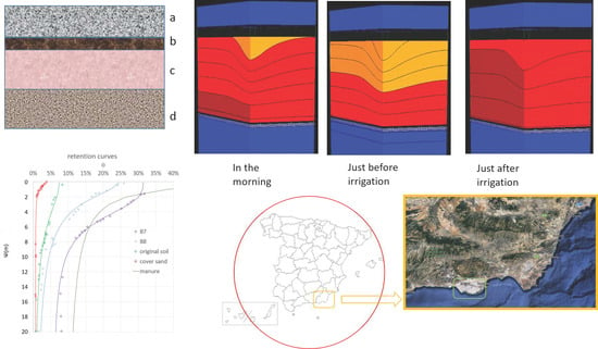
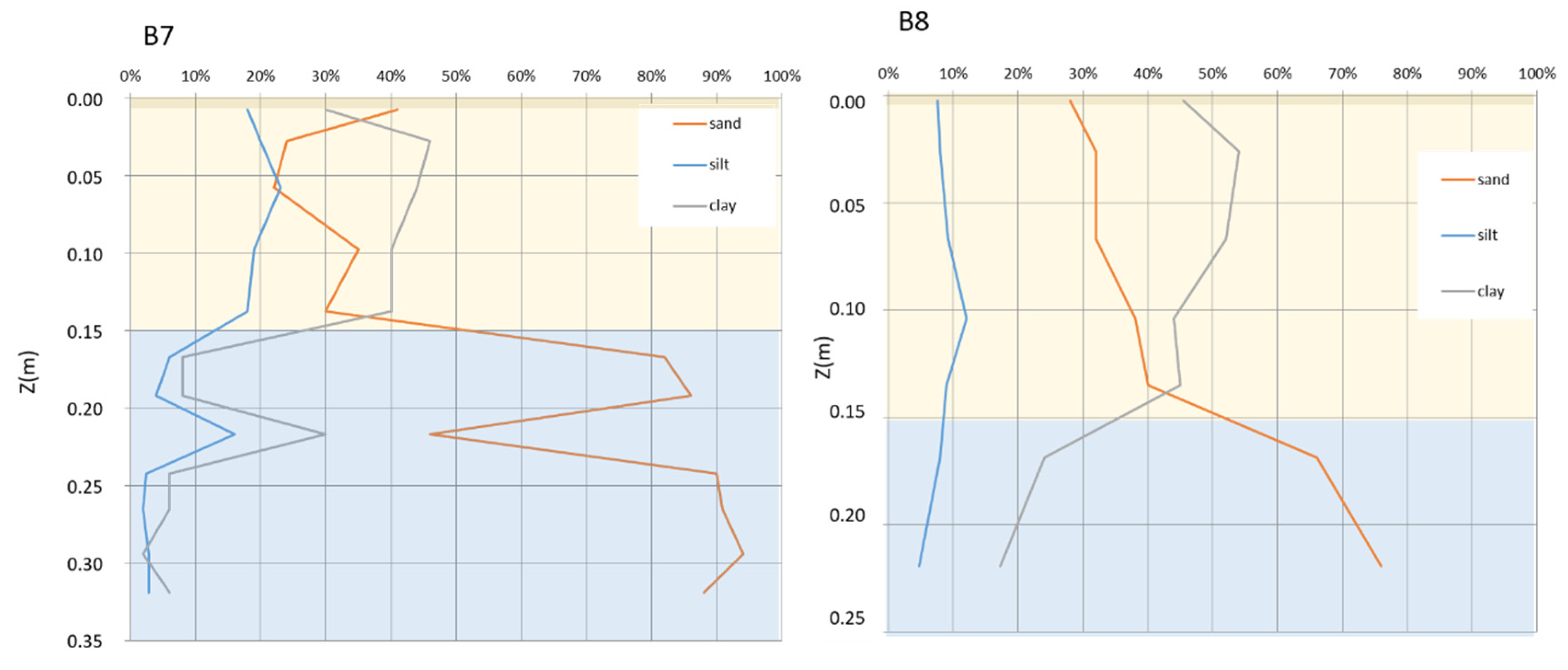
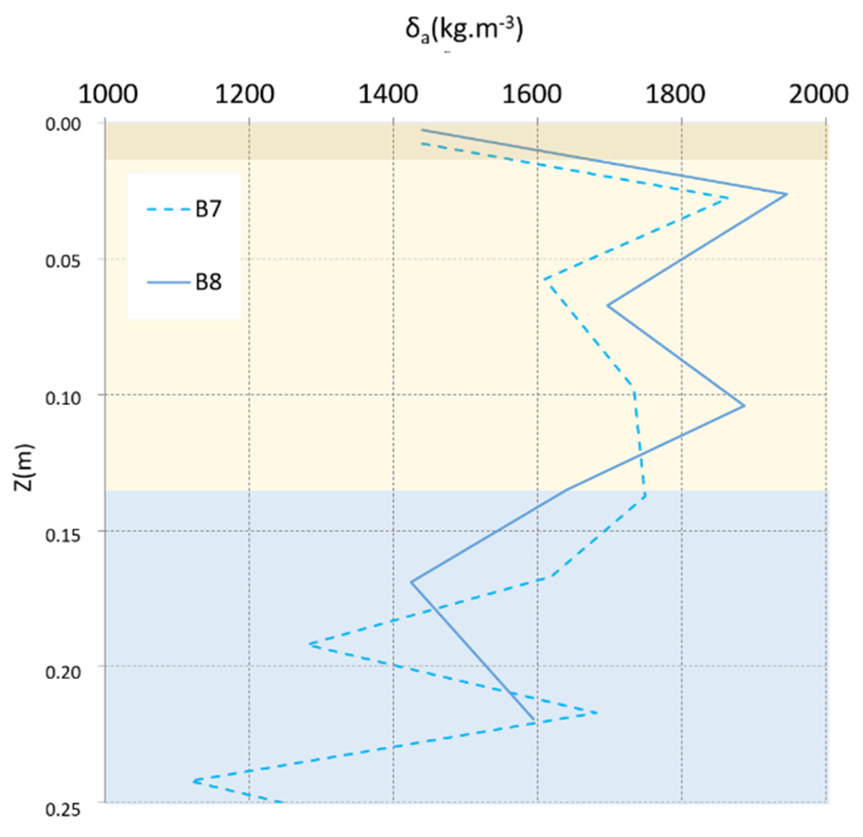
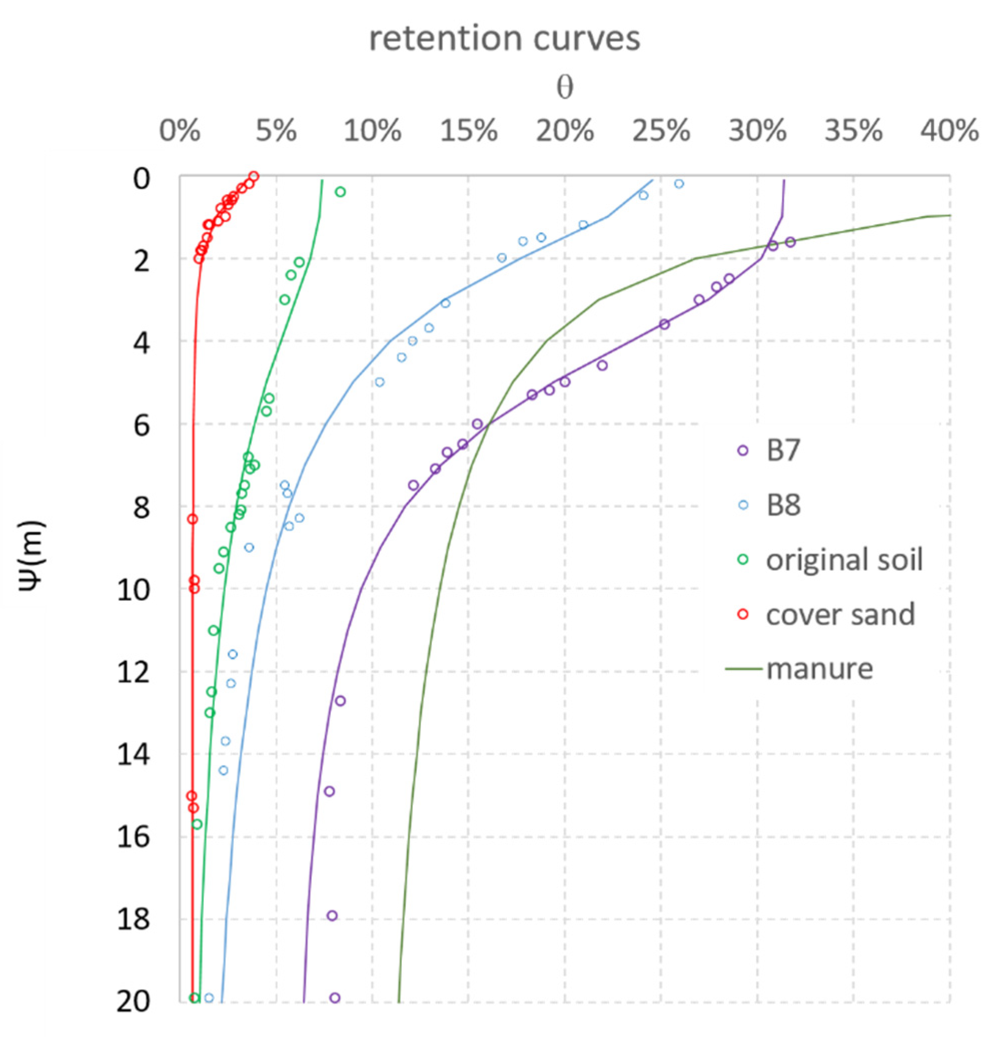
3.1. Moisture Retention Curve of Greenhouse Soils

Once the values specified in the methodology have been measured, the theoretical curves have been calibrated. To do this, the least-squares adjustment of Equation (1) is performed, using the Excel Solver routine to find the best values of the parameters θs, θr, α, and n.

Table 2. Van Genuchten curve parameters obtained by the least squares adjustment procedure. δa, ks and Index of agreement, Ia, for the best fit is also given.

	B7	B8	Original Soil	Organic Matter	Cover Sand
θs (%)	31.99	24.56	7.403	89.50	3.51
θr (%)	5.62	0.00	0.00	8.69	0.63
α (m−1)	2.24 × 10−7	4.72 × 10−7	2.33 × 10−7	2.7 × 10−6	1.496 × 10−6
n	3.310	2.077	2.282	1.391	2.593
δa (kg·m−3)	1740	1490	1790	1440	1510
ks(m·s−1)	2.93 × 10−8	6 × 10−7	1.2858 × 10−5	2.199 × 10−5	9.334 × 10−4
Ia (%)	99.97	99.84	99.39	99.70	98.20

shows these values, as well as the bulk density δa and the Index of agreement, Ia, for the best fit. The moisture measurements were made on weight values and have subsequently been converted to volumetric values by means of the measured bulk density and considering apparent volume of the sample. Organic matter parameters were obtained from bibliography [47].

Figure 7 shows the point cloud of the measured data (moisture in weight) and the best fitting curve for each material.

3.2. Estimation of Water Movement Using the Hydrus-3D Program

With the data and measured curves, the information that the Hydrus-3D model needs is provided. This operation resulted in the definition of a simple multi-layered 3D model. The most superficial layer, 0.050 m thick, will be of coarse sand with the properties measured for this material. The layer of organic matter is 0.005 m, in line with what was observed in the experimental plot. The layer of material provided will be 0.150 m, which is the average thickness observed in the experimental plots. A very thick layer (>0.800 m) has also been prepared with the characteristics of the original material.

The simulations were implemented in simple 3D geometry, with lengths in mm, and the working block size was 0.250 × 0.600 × 1.000 m. The processes activated were water flow and root water extraction. For water extraction by the roots, the Feddes option was used with P0 = −0.100 m, P0pt = −0.250 m, P2H = −8.000 m, P2L = −15.000 m, P3 = −80.000 m, r2H = 5.787 × 10⁻⁸ m·s⁻¹, and r2L = 1.1566 × 10⁻⁸ m·s⁻¹. The time unit was minutes up to a total of 2880, with 144 variable boundary values, every 20 min each, coming from data taken by a nearby weather station inside a similar greenhouse. Figure 8 shows the evapotranspiration data used as boundary variable values.

The maximum number of iterations was set at 20, with a 0.001 tolerance for moisture content and 0.010 m for tension. The initial condition was established as a constant stress of 0.500 m throughout the profile.

It has been observed that the initial soil conditions can only be set as a constant value for each depth. Since the initial soil conditions should be variable in the 3 dimensions of space, two consecutive days in February were chosen to reproduce this situation, of which the hourly evaporation is known and whose irrigation episode occurred on the second day. In this way, it is possible to reach the beginning of the second day with variable tension conditions around the emitter and the plant. The irrigation programmed for the crop, once the tension of ψ = 1.000 m is reached, is always 20 min long.

In the localized irrigation process, a small-saturated zone is formed under the dripper from which the infiltration takes place [13]. In line with the findings of other authors [29], some instability of the model has been observed when the flow was too high. For this reason, a variable flow source 1.333 × 10⁻⁴ m·s⁻¹, corresponding to a quarter of the emitter’s flow in a surface of 0.0015625 m² was applied. This simulates a quarter of the soil, since the model places the root in the coordinates (0.0) of the simulated block by default. For the lateral surfaces and the bottom of the prism, it was considered that the most appropriate boundary condition was that of no flow, whose main characteristic is that water would not pass through this surface. Given the conditions of the test and taking into account that both the emitter and plant are located in the upper left corner, it was considered the most appropriate condition. The upper surface was considered under atmospheric conditions. To adjust the model, different initial tension values were proposed, uniform throughout the profile, with the requirement that, at the time of irrigation, the expected tension of ψ = 1.000 m should be reached at the position of the tensiometer. The recorded time of irrigation on the chosen day, 10 February 2018, was 15:00 h and the simulation began at 00:00 h the previous day. Therefore, irrigation starts at time t = 2340 min.

As an example, in Figure 9, critical moments of the day are selected. As commented, the simulation is started the day before so that the day to be simulated finds the pressure conditions correctly distributed in the 3 dimensions. The beginning of the day is presented at minute 1440 of the simulation, which corresponds to midnight. The effect of the water extraction by the crop on the previous day persists. The beginning of the day, and consequently, the beginning of the crop’s evapotranspiration occurs at minute 1800 of the simulation. It can be observed that the humidity has been redistributed and the profile presents an almost homogeneous humidity. In minute 2180, a remarkable extraction by the crop has already been reached, which reaches its greatest extension in minute 2320, when the irrigation takes place (the irrigation starts in minute 2340). From there, areas with a moisture deficit are filled from the water provided and from the redistribution from other points of the profile. At the end of the day a situation very similar to that of the beginning has been reached.

The thermal oscillation and the evaporation, inside a greenhouse, remain very similar for different days of February. For this example, any day was chosen when an irrigation was applied.

A series of observation points were defined in the model, coinciding with the positions of the probes installed in the field, in order to compare the field measurements with the values predicted by the Hydrus-3D model. Figure 10 shows the simulated (S) with Hydrus-3D and values measured (M) with the probes, shown in series of the same color, follow the same evolution. A similar behavior was observed in a vineyard [48] using a procedure like the one presented in this work.

Although measurements are available every second, some of them have been removed to make the dots on the graph more visible.

The slope of the simulated vs. measured value line and the adjustment index for each observation point tested, are shown in

Table 3. Slope m of the simulated vs. measured value line passing through the origin and adjustment index, Ia, for a series of probes.

	P5	P2	P8	P6	P3	P10–P9	P7	P4–P1
m(0,0)	0.990	0.999	1.002	0.993	1.002	1.004	0.996	0.995
Ia	1.000	0.997	0.988	1.000	1.000	1.000	1.000	0.999

and suggest an adequate representation of water movement in this type of soil.

For the fitting of the model, the condition that the moment in which the set point tension was reached in the place where the tensiometer was placed. For this test, the tensiometer was placed 0.130 m from the dripper and 0.130 m perpendicular to the drip line. The depth of the capsule was 0.100 to 0.150 m measured below the surface of the soil provided. Figure 11 shows the evolution of tension (m) for 0.130 m depth below the surface of the added soil (z = 0.180 m from the soil surface).

It can be seen that the 1.000 m tension line passes through the position of the tensiometer approximately at the time when irrigation started. The tension conditions are maintained for a few minutes and by midnight, the initial conditions have been recovered.

Once the model was adjusted for both soils, the influence of root distribution on the evolution of moisture and tension was studied. Figure 12 shows the tension distribution for t = 2320 min (just before irrigation) for the two crops in both soils and in several sections of the crop profile. We selected z = 0.060 m, right in the organic matter layer, z = 0.100 m, where the most superficial probes were placed, z = 0.180 m, in position of the tensiometer capsule that directs the irrigation operation, and z = 0.200 m, where the deepest probes were placed.

In the figure, the influence of the soil type can be clearly seen, which configures the general stress state of the soil water, as was to be expected in view of the parameters of the retention curves.

4. Discussion

There seem to be differences between the different substrates. Soil B8 contains more gravel and this seems to determine a more irregular distribution of moisture. In practice, it is to be expected that no differences appear between the measurements of the probes. If we add to this the differences in the calibration of the probe itself, the data should not show clear differences, as is the case in practice.

Considering the evolution of soil moisture (Figure 8), the clayey texture of both soils, together with the effect of the organic layer, makes the humidity spread rapidly through the soil layers and, after watering, the humidity reaches an almost constant value. There are times of the year in which a predictable distribution appears, in which the most humid area is around the dripper, but there are other times, coinciding with the complete development of the plant, in which a drying area appears around the plant or no recognizable distribution appears. This behavior coincides with that observed by Coelho and Dani [49] in corn. This circumstance sheds light on the importance of the extraction of the plant in intensive layered soil crop systems.

4.1. Moisture Retention Curve of Greenhouse Soils

The soil sample B7 was subdivided into two subsamples corresponding to consecutive depth parts of the core taken from the profile. It can be observed that soils B7-a and B7-b are practically the same, which seems to confirm that the profile is homogeneous. The two soils, B7 and B8, also show a similar curve, in spite of their textural differences. The bases also show the same behavior which is in line with the fact that the two substrates are almost identical in terms of texture. The sand cover, due to its granulometry, presents an extreme retention curve, in the sense that its capacity to store water is very low and falls very quickly when the tension increases, even slightly. Some authors [50] have found similar behavior in mulching materials. These results are consistent with the estimates made based on the texture of each sample (see Figure 7).

4.2. Estimation of Water Movement Using the Hydrus-3D Program

In general, the model predicts well the behavior of moisture in the conditions posed. On the other hand, the model predicts smoother variations in moisture than those recorded in the field. This behavior may be because the roots increase the heterogeneity of the soil and the variations in humidity are somewhat amplified.

The results show that the heavier B7 soil causes greater tension throughout the profile for both crops. On the other hand, the sweet pepper crop occupies the soil and causes a great tension gradient around the plant.

The observed behavior implies that the set point tension is reached earlier in heavy soils, such as B7. For this type of soil, a higher set point tension or a wider distance of the tensiometer from the plant is recommended so that the watering frequency would not be excessive. Some researchers trying to determine the optimum stress point for a crop came to the same conclusion [51], although in this case they worked with sandy soils.

Although high irrigation efficiencies are achieved in this geographical area, the study shows that it is possible to improve irrigation management, reduce water consumption, and therefore reduce pollutants from agricultural practice. In summary, the knowledge of wet bulb distribution according to the type of soil, can allow farmers to establish future irrigation strategies, and promote a more resilient greenhouse agriculture.

5. Conclusions

A procedure was defined for collecting and processing moisture data in layered soils.

It proceeded to reproduce in the model Hydrus-3D the conditions of behavior of a layered soil and it was possible to verify that the predictions were adapted to what has been observed. It was thus defined that the procedure could adequately simulate the evolution of moisture in stratified “sanded” soils used in intensive horticultural greenhouse crops under the usual irrigation conditions in this area.

It was found that the inclusion of a previous day in the simulation improved model predictions of soil moisture distribution.

Under the conditions of the test and with a correct adjustment of the soil and root parameters, the Hydrus model could adequately predict the moment when the tensiometer launched the irrigation process, which allowed it to be used to optimize the control of the irrigation process.

In soils with less gravel, a lower average stress and a more homogeneous moisture distribution were observed.

In view of the results, the Hydrus-3D model could be used to establish future irrigation strategies or to locate the optimal placement point of tensiometers that control irrigation in sanded soils for intensive agriculture.

References

1. Chico, D.; Salmoral, G.; Llamas, M.R.; Garrido, A.; Aldaya, M.M. The Water Footprint and Virtual Water Exports of Spanish Tomatoes; Fundación Botín: Madrid, Spain, 2010; Volume 8. [Google Scholar]
2. Neira, D.P.; Montiel, M.S.; Cabeza, M.D.; Reigada, A. Energy use and carbon footprint of the tomato production in heated multi-tunnel greenhouses in Almeria within an exporting agri-food system context. Sci. Total Environ. 2018, 628–629, 1627–1636. [Google Scholar] [CrossRef]
3. Modaihsh, A.S.; Horton, R.; Kirkham, D. Soil Water Evaporation Suppression by Sand Mulches. Soil Sci. 1985, 139, 357–361. [Google Scholar] [CrossRef]
4. Wang, Y.; Xie, Z.; Sukhdev, S.; Vera, C.L.m.; Zhang, Y.; Guo, Z. Effects of gravel–sand mulch, plastic mulch and ridge and furrow rainfall harvesting system combinations on water use efficiency, soil temperature and watermelon yield in a semi-arid Loess Plateau of northwestern China. Agric. Water Manag. 2011, 101, 88–92. [Google Scholar] [CrossRef]
5. Bonachela, S.; López, J.C.; Granados, M.R.; Magán, J.J.; Hernández, J.; Baille, A. Effects of gravel mulch on surface energy balance and soil thermal regime in an unheated plastic greenhouse. Biosyst. Eng. 2020, 192, 1–13. Available online: http://www.sciencedirect.com/science/article/pii/S1537511020300222 (accessed on 19 February 2021). [CrossRef]
6. Pérez, J.; López, J.; Fernández, M.D. La Agricultura del Sureste: Situación Actual y Tendencias de las Estructuras de Producción en la Horticultura Almeriense 2a. Edición; Editorial Caja Rural Intermediterránea: Madrid, Spain, 2002. [Google Scholar]
7. Arbat, G.; Puig-Bargués, J.; Duran-Ros, M.; Barragán, J.; De Cartagena, F.R. Drip-Irriwater: Computer software to simulate soil wetting patterns under surface drip irrigation. Comput. Electron. Agric. 2013, 98, 183–192. [Google Scholar] [CrossRef]
8. Singh Lubana, P.P.; Narda, N.K. Soil and Water: Modelling Soil Water Dynamics under Trickle Emitters—A Review. J. Agric. Eng. Res. 2001, 78, 217–232. Available online: http://www.sciencedirect.com/science/article/pii/S0021863400906504 (accessed on 7 February 2013). [CrossRef]
9. Schwartzman, M.; Zur, B. Emitter spacing and geometry of wetted soil volume. J. Irrig. Drain. Eng. 1986, 112, 242–253. [Google Scholar] [CrossRef]
10. Amin, M.S.M.; Ekhmaj, A.I.M. DIPAC-Drip Irrigation Water Distribution Pattern Calculator. In Proceedings of the 7th International Micro Irrigation Congress, Pwtc, Kuala Lumpur, Malaysia, 10–16 September 2006. [Google Scholar]
11. Kandelous, M.M.; Šimůnek, J. Comparison of numerical, analytical, and empirical models to estimate wetting patterns for surface and subsurface drip irrigation. Irrig. Sci. 2010, 28, 435–444. [Google Scholar] [CrossRef] [Green Version]
12. Philip, J.R. Steady infiltration from buried, surface and perched point and line sources in heterogeneous soils, I. Analysis. Soil Sci. Soc. Am. Proc. 1972, 36, 268–273. [Google Scholar] [CrossRef]
13. Chu, S.-T. Geen-Ampt Analysis of wetting patterns for surface emitters. J. Irrig. Drain Eng. 1994, 120, 414–421. [Google Scholar] [CrossRef]
14. Hill, D.E.; Parlange, J.-Y. Wetting Front Instability in Layered Soils. Soil Sci. Soc. Am. J. 1972, 36, 697–702. [Google Scholar] [CrossRef]
15. Li, Z.; VanderBorght, J.; Smits, K.M. The effect of the top soil layer on moisture and evaporation dynamics. Vadose Zone J. 2020, 19, 10. [Google Scholar] [CrossRef]
16. Garcia-Caparros, P.; Contreras, J.I.; Baeza, R.; Segura, M.L.; Lao, M.T. Integral Management of Irrigation Water in Intensive Horticultural Systems of Almería. Sustainability 2017, 9, 2271. [Google Scholar] [CrossRef] [Green Version]
17. Fernández, J.E.; Moreno, F.; Cabrera, F.; Arrúe, J.L.; Martin-Aranda, J. Drip irrigation, soil characteristics and the root distribution and root activity of olive trees. Plant Soil 1991, 133, 239–251. [Google Scholar] [CrossRef]
18. Newman, E.I. A Method of Estimating the Total Length of Root in a Sample. J. Appl. Ecol. 1966, 3, 139. [Google Scholar] [CrossRef]
19. Steudle, E. Water uptake by plant roots: An integration of views. Plant Soil 2000, 226, 45–56. [Google Scholar] [CrossRef]
20. Prasad, R. A linear root water uptake model. J. Hydrol. 1988, 99, 297–306. [Google Scholar] [CrossRef]
21. Šimunek, J.; Van Genuchten, M.T.; Šejna, M. HYDRUS: Model use, calibration, and validation. Trans. ASABE 2012, 55, 1263–1274. [Google Scholar]
22. Richards, L.A. Capillary conduction of liquids through porous mediums. Physics 1931, 1, 318–333. [Google Scholar] [CrossRef]
23. Simunek, J. Modeling Water Flow and Contaminant Transport in Soils and Groundwater Using the HYDRUS Computer Software Packages; International Groundwater Modeling Center, Colorado School of Mines: Golden, CO, USA, 2006; pp. 12–28. [Google Scholar]
24. Sasidharan, S.; Bradford, S.A.; Šimůnek, J.; Kraemer, S.R. Groundwater recharge from drywells under constant head conditions. J. Hydrol. 2020, 583, 124569. [Google Scholar] [CrossRef]
25. Crevoisier, D.; Popova, Z.; Mailhol, J.; Ruelle, P. Assessment and simulation of water and nitrogen transfer under furrow irrigation. Agric. Water Manag. 2008, 95, 354–366. [Google Scholar] [CrossRef] [Green Version]
26. Honar, M.R.; Shamsnia, S.A.; Gholami, A. Evaluation of water flow and infiltration using HYDRUS model in sprinkler irrigation systems. In Proceedings of the 2nd International Conference on Environmental Engineering and Applications, Shanghai, China, 19 August 2011; Volume 17. [Google Scholar]
27. Kandelous, M.M.; Šimůnek, J. Numerical simulations of water movement in a subsurface drip irrigation system under field and laboratory conditions using HYDRUS-2D. Agric. Water Manag. 2010, 97, 1070–1076. [Google Scholar] [CrossRef]
28. Provenzano, G. Using HYDRUS-2D Simulation Model to Evaluate Wetted Soil Volume in Subsurface Drip Irrigation Systems. J. Irrig. Drain. Eng. 2007, 133, 342–349. [Google Scholar] [CrossRef]
29. ElNesr, M.; Alazba, A. Computational evaluations of HYDRUS simulations of drip irrigation in 2D and 3D domains (ii-subsurface emitters). Comput. Electron. Agric. 2019, 163, 104879. [Google Scholar] [CrossRef]
30. Domínguez-Niño, J.M.; Arbat, G.; Raij-Hoffman, I.; Kisekka, I.; Girona, J.; Casadesús, J. Parameterization of Soil Hydraulic Parameters for HYDRUS-3D Simulation of Soil Water Dynamics in a Drip-Irrigated Orchard. Water 2020, 12, 1858. [Google Scholar] [CrossRef]
31. Shan, Y.; Wang, Q. Simulation of salinity distribution in the overlap zone with double-point-source drip irrigation using HYDRUS-3D. Aust. J. Crop Sci. 2012, 6, 238. [Google Scholar]
32. Mao, X.M.; Shang, S.H. Method of minimum flux in saturation layer for calculating stable water infiltration through layered soil. J. Hydraul. Eng. 2010, 41, 810–817. [Google Scholar]
33. Ma, Y.; Feng, S.; Su, D.; Gao, G.; Huo, Z. Modeling water infiltration in a large layered soil column with a modified Green–Ampt model and HYDRUS-1D. Comput. Electron. Agric. 2010, 71, S40–S47. [Google Scholar] [CrossRef]
34. Tan, X.; Shao, D.; Gu, W.; Liu, H. Field analysis of water and nitrogen fate in lowland paddy fields under dif-ferent water managements using HYDRUS-1D. Agric. Water Manag. 2015, 150, 67–80. [Google Scholar] [CrossRef]
35. Antonov, D.; Mallants, D.; Šimůnek, J.; Karastanev, D. Application of the HYDRUS (2D/3D) Inverse Solution Module for Estimating the Soil Hydraulic Parameters of a Quaternary Complex in Northern Bulgaria. In Proceedings of the HYDRUS Software Applications to Subsurface Flow and Contaminant Transport Problems, Prague, Czech Republic, 21–22 March 2013; p. 47. [Google Scholar]
36. Mohammed, A.K.; Abed, B.S. Water distribution and interference of wetting front in stratified soil under a continues and an intermittent subsurface drip irrigation. J. Green Eng. 2020, 10, 268–286. [Google Scholar]
37. Becerra, A.T.; Bravo, X.B.L.; Membrive, V.J.F. Huella hídrica y sostenibilidad del uso de los recursos hídricos. M A Rev. Electrónica Medioambiente 2013, 14, 56. [Google Scholar]
38. Bouyoucos, G.J. Directions for making mechanical analyses of soils by the hydrometer method. Soil Sci. 1936, 42, 225–230. [Google Scholar] [CrossRef]
39. Brooks, R.; Corey, T. Hydraulic Properties of Porous Media; Hydrology Papers n° 3, Fort Collings; Colorado State University: Fort Collins, CO, USA, 1964. [Google Scholar]
40. Van Genuchten, M.T. A Closed-form Equation for Predicting the Hydraulic Conductivity of Unsaturated Soils. Soil Sci. Soc. Am. J. 1980, 44, 892–898. [Google Scholar] [CrossRef] [Green Version]
41. Vrugt, J.A.; Hopmans, J.W.; Šimůnek, J. Calibration of a Two-Dimensional Root Water Uptake Model. Soil Sci. Soc. Am. J. 2001, 65, 1027–1037. [Google Scholar] [CrossRef]
42. Vrugt, J.A.; Van Wijk, M.T.; Hopmans, J.W.; Šimunek, J. One-, two-, and three-dimensional root water uptake functions for transient modeling. Water Resour. Res. 2001, 37, 2457–2470. [Google Scholar] [CrossRef] [Green Version]
43. Zapata-Sierra, A.; Pérez, M.M.; Requena, R.R.; Manzano-Agugliaro, F. Root distribution with the use of drip irrigation on layered soils at greenhouses crops. Sci. Total. Environ. 2021, 144944. [Google Scholar] [CrossRef]
44. Willmott, C.J. ON THE VALIDATION OF MODELS. Phys. Geogr. 1981, 2, 184–194. [Google Scholar] [CrossRef]
45. Zapata-Sierra, A.J.; López-Segura, J.G.; Cánovas-Fernández, G.; Baeza-Cano, R. Caracterización del bulbo mojado por un gotero en suelos arenados mediante sondas fdr. In XXXVI Congreso Nacional de Riegos, Valladolid; Colegio Oficial de Ingenieros Agronomos de Centro y Canarias: Madrid, Spain, 2018; pp. 1–8. [Google Scholar] [CrossRef]
46. Zapata-Sierra, A.J.; Contreras, J.; Usero, F.; Baeza, R. Influencia de la textura del suelo en los bulbos húmedos desarrollados en suelo enarenado con emisores de riego localizado de bajo caudal. In XXXIII Congreso Nacional de Riegos; Universitat Politecnica de Valencia: Valencia, Spain, 2015; pp. 74–84. [Google Scholar] [CrossRef] [Green Version]
47. Sutitarnnontr, P.; Hu, E.; Tuller, M.; Jones, S.B. Physical and Thermal Characteristics of Dairy Cattle Manure. J. Environ. Qual. 2014, 43, 2115–2129. [Google Scholar] [CrossRef]
48. Zhou, Q.; Kang, S.; Zhang, L.; Li, F. Comparison of APRI and Hydrus-2D models to simulate soil water dynamics in a vineyard under alternate partial root zone drip irrigation. Plant Soil 2007, 291, 211–223. [Google Scholar] [CrossRef]
49. Coelho, E.F.; Or, D. Root distribution and water uptake patterns of corn under surface and subsurface drip irrigation. Plant Soil 1998, 206, 123–136. [Google Scholar] [CrossRef]
50. Tejedor, M.; Jimenez, C.; Díaz, F. Volcanic materials as mulches for water conservation. Geoderma 2003, 117, 283–295. [Google Scholar] [CrossRef]
51. Caron, J.; Bonin, S.; Pepin, S.; Kummer, L.; Vanderleest, C.; Bland, W.L. Determination of irrigation set points for cranberries from soil- and plant-based measurements. Can. J. Soil Sci. 2016, 96, 37–50. [Google Scholar] [CrossRef] [Green Version]
Figure 1. Diagram of layered soil. (a) Sand cover, (b) organic matter, (c) added crop soil, and (d) original soil.
Water 13 00600 g001
Figure 2. Location of the tests.
Water 13 00600 g002
Figure 3. Arrangement of paired lanes typical of intensive agriculture (units in m). Water 13 00600 i001 Indicates probes position.
Water 13 00600 g003
Figure 4. Fine fraction texture of soils B7 and B8, used in the tests.
Water 13 00600 g004
Figure 5. Variation of bulk density δa (kg·m−3) as a function of depth for soils B7 and B8.
Water 13 00600 g005
Figure 6. Arrangement and numbering of the probes in soil B8. ( Water 13 00600 i002 z = 0.050 m, Water 13 00600 i003, z = 0.150 m).
Water 13 00600 g006
Figure 7. Best-fit point cloud and moisture retention curve for the soils tested.
Water 13 00600 g007
Figure 8. Time variable boundary conditions for 9 and 10 February 2018.
Water 13 00600 g008
Figure 9. Evolution of soil moisture (fraction) simulated with Hydrus-3D for a day of cultivation and irrigation operation of 20 min. Variation over the second full day is shown. Sweet pepper soil B8.
Water 13 00600 g009
Figure 10. Evolution of measured (M) and simulated with Hydrus-3D (S) soil moisture for 10 February, 2018. Numbered probes according to the distribution in Figure 6.
Water 13 00600 g010
Figure 11. Tension evolution (m) for 10 February 2018. The position of the tensiometer is shown with a red cross +. Soil B8, 0.130 m depth in the added soil layer.
Water 13 00600 g011
Figure 12. Soil water tension simulated by Hydrus-3D for different soil depths for t = 2320 min for sweet pepper in soils B7 and B8.
Water 13 00600 g012