
Quantifying the Response of Grass Carp Larvae to Acoustic Stimuli Using Particle-Tracking Velocimetry

Department of Civil and Environmental Engineering, University of Illinois At Urbana-Champaign, 205 N Mathews Ave. M/C 250, Urbana, IL 61801, USA
*
Author to whom correspondence should be addressed.
Water 2021, 13(5), 603; https://doi.org/10.3390/w13050603
Submission received: 8 January 2021
/
Revised: 17 February 2021
/
Accepted: 19 February 2021
/
Published: 25 February 2021
(This article belongs to the Section Biodiversity and Functionality of Aquatic Ecosystems)
Abstract
:Acoustic deterrents are recognized as a promising method to prevent the spread of invasive grass carp, Ctenopharyngodon idella (Valenciennes, 1844) and the negative ecological impacts caused by them. As the efficacy of sound barriers depends on the hearing capabilities of carp, it is important to identify whether carps can recognize acoustic signals and alter their swimming behavior. Our study focuses on quantifying the response of grass carp larvae when exposed to out-of-water acoustic signals within the range of 100–1000 Hz, by capturing their movement using particle-tracking velocimetry (PTV), a quantitative imaging tool often used for hydrodynamic studies. The number of responsive larvae is counted to compute response ratio at each frequency, to quantify the influence of sound on larval behavior. While the highest response occurred at 700 Hz, we did not observe any clear functional relation between frequency of sound and response ratio. Overall, 20–30% of larvae were consistently reacting to sound stimuli regardless of the frequency. In this study, we emphasize that larval behaviors when exposed to acoustic signals vary by individual, and thus a sufficient number of larvae should be surveyed at the same time under identical conditions, to better quantify their sensitivity to sound rather than repeating the experiment with individual specimens. Since bulk quantification, such as mean or quantile velocities of multiple specimens, can misrepresent larval behavior, our study finds that including the response ratio can more effectively reflect the larval response.
1. Introduction
Grass carp, Ctenopharyngodon idella (Valenciennes, 1844) were originally imported from Asia to the Mississippi River Basin for control of macrophytes. Nowadays, they are one of the most notorious invasive species of aquaculture in the central United States [1]. Different types of barrier and deterrent have been proposed to control the spread of such invasive species. However, the efficacy of each strategy still remains inconclusive and requires further investigation [2,3,4]. Among them, sound barriers are typical non-physical barriers which inject traveling pressure waves as a stimulus to block carp passage and confine their habitat [4]. Sound barriers are relatively easy to implement at relatively low cost, without causing any physical change in water flow or damaging the surrounding environment, which makes them a promising strategy to control invasive carp species [3].
Another advantage of acoustic stimuli is that carps have greater capacity to detect a wide frequency range of sound compared to most fish inhabiting in Midwest Rivers, which could allow for the design of selective acoustic barriers targeting only invasive species [5,6,7]. Common Midwestern fishes such as Lake Sturgeon, Acipenser fulvescens (Rafinesque, 1817) and Bluegill Sunfish, Lepomis macrochirus (Rafinesque, 1819) detect sound up to 400 Hz in maximum, while carps can hear much broader frequency range depending on their taxonomy [6,8]. It has been reported that both Silver carp, Hypophthalmichthys molitrix (Valenciennes, 1844) and bighead carp, Hypophthalmichthys nobilis (Richardson, 1845) can detect up to 5000 Hz for pure tones and can even go further for mixed tones [9]. Grass carp, in particular, have shown to alter their behavior in response to sounds of up to 1000 Hz [10,11].
Despite research efforts focused on the hearing ability of carp, the most effective frequency range of acoustic stimuli has not been yet defined. One major challenge is that results are highly dependent on experimental conditions, and the various techniques to define and analyze the response of individual specimens [9,10,11,12]. A consistent, robust experimental method is needed to apply to various circumstances with high reliability. In addition, compared to active research on hearing capabilities of mature carp, much less is known about the frequency range that carp can perceive, and respond to, during their early developmental stages [13]. The reproduction strategy of grass carp is to release eggs directly into the ambient water and let them drift until hatched larvae find habitats suitable for their growth [5]. If the navigation of carp larvae can be controlled with acoustic stimuli, it can limit the spread of carp from their early stages.
The main objective of this study is to analyze the behavior of grass carp larvae exposed to sound of different frequencies, using proven quantitative imaging techniques used in hydrodynamic studies, to obtain reliable conclusions about the relation between sound frequency and larvae response. We introduce a robust framework to quantify the response to acoustic signals by capturing their movements with a camera and identifying trajectories via particle-tracking velocimetry (PTV). The response of grass carp larvae to external (i.e., out-of-water) acoustic signals of 100 to 1000 Hz frequency range are analyzed based on two quantities: 1) bulk velocities at each frame computed by averaging the velocity of every larvae and 2) response ratio computed from the number of larvae experiencing large variation of velocities and acceleration at the tone frame.
2. Materials and Methods
2.1. Experimental Design
Fertilized grass carp eggs were collected and transported as described in Prada et al. [14]. All procedures were authorized by the Illinois Department of Natural Resources. Larvae hatched in a recirculating flume at a controlled temperature of 23–24 °C and stayed there for 5 days (reaching developmental stages 37–39) before the present experiment to ensure that larvae developed an ability to swim and were able to displace to their preferred locations [14,15].
Experiments were conducted at the Ven Te Chow Hydrosystems Laboratory (VTCHL), at the University of Illinois at Urbana Champaign. Approximately 200 larvae were placed inside a fish tank with dimensions 0.5 m long and 0.25 m wide, with a water depth of 0.075 m. After an acclimation period, the response of larvae to acoustic stimuli was tested. Since we are interested in their response to external noise (i.e., environmental noise generated out of the water in the stream, rather than a signal generated underwater), we used computer speakers (Logitech LS21) installed outside of the tank as our source. Acoustic stimuli consisted of single tones ranging from 100–1000 Hz, varying in 100 Hz increments with a constant amplitude of 60 dB. The tones were generated using Matlab’s ‘sound’ function, creating a sinusoidal signal with the respective frequency between 100–1000 Hz. Each signal lasted for 1 s for every case. Reactions were recorded with two GoPro Hero 4 Black cameras (4K resolution, frame size of 3840 × 2160 pixels, 30 frames per second), installed above and to the side of the fish tank. Recording started 5 s prior to the sound and continued for another 5 s after the sound was ceased to capture baseline and recovery images.
2.2. Acquisition of Larval Trajectories
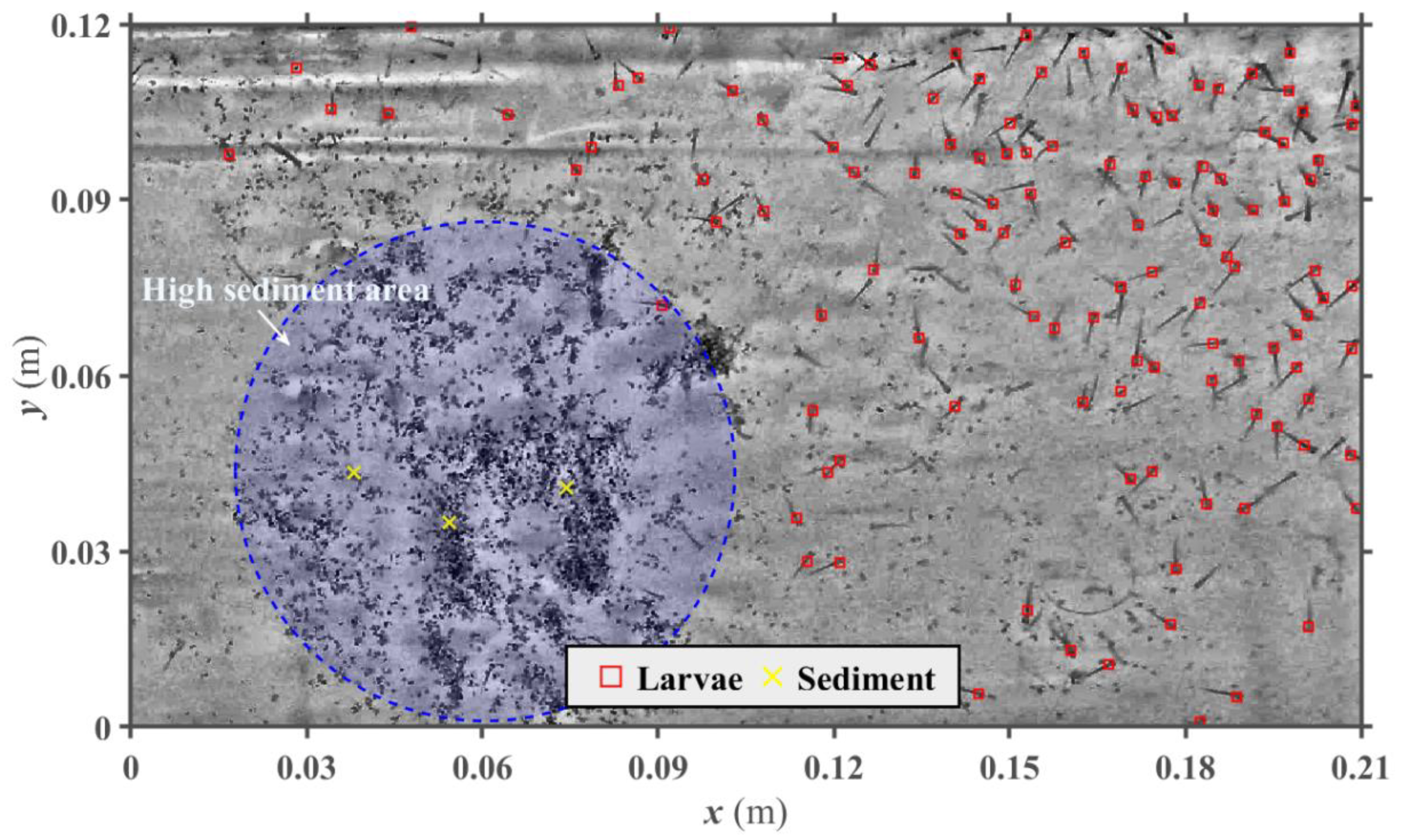
Recordings from a top-view camera were processed using a custom particle image processing Matlab routine to obtain larvae trajectories based on a two-stage process: (1) identification of larvae from individual frames and (2) matching larvae between two consecutive frames [16]. Raw videos were converted into time series of individual grayscale frames. The background was removed through an image-preprocessing procedure to only leave motile larvae on the image. The larvae were initially specified as circular shapes without considering their tails, defining a radius of 2.5 mm (similar dimension as matured eggs, e.g., [5,17,18]). While other geometries were considered, the spherical approach performed better at both recognizing a larger number of larvae (Figure 1) and experiencing a smaller “loss” of larvae between frames (i.e., missing a larva on consecutive frames if a larva moves or changes orientation). The spherical approach yielded the coordinates of the larvae centroids in each frame, which allowed us to proceed with particle matching for displacement calculations.
Figure 1 (top-view camera) shows the location where larvae were detected from an individual image, focusing on a highly populated region inside the fish tank. Although the algorithm missed some larvae, the majority was captured by their heads, and even closely located larvae were distinguished from each other as separate objects. The algorithm was also successful to capture larvae while neglecting other elements on the image, such as sediment and light reflections. While sediment grains were present in the fish tank (circle shown in Figure 1), only a few were mis-identified as larvae (yellow cross-marks in Figure 1).
In the second stage of the routine, the matching algorithm searched for larvae in consecutive frames to build trajectories over time, limited by a maximum distance that larvae can travel between two frames, and using the distribution of pixel intensities around larvae centroids for identification and matching. Since the experiment was conducted with still water conditions, the algorithm solely depended on larvae movements between two consecutive frames without considering any surrounding flow speeds. Displacements of larvae were quantified by velocity and acceleration based on the assumption that vertical movements are negligible, and larvae are moving in the horizontal plane. We use the magnitudes of velocity and acceleration, computed considering the components in the x and y directions. For consistency of the analysis, positions of larvae were tracked at identical numbers of images (30 frames) corresponding to prior to the sound stimuli, throughout the sound exposure and after the sound ceased. The instantaneous velocity and acceleration of larvae at each frame were quantified based on their displacement between frames.
2.3. Quantification of Larval Response to Sound Stimuli
The bulk behavior of larvae when exposed to abrupt sound stimuli are quantified by their velocity statistics at each frame. Mean velocity represents the overall movements of every identified larvae. To account for the largest displacements between frames, a 95th percentile was used to only account for extreme velocities, which reflects behaviors of larvae that are most active or sensitive to surrounding environments. Mean velocity and the 95 percentile are calculated based on Equations (1) and (2), respectively, where is the mean velocity, is the total number of larvae, is the velocity of larva and is the rank of velocity to satisfy the 95th percentile (i.e., the 95th percentile, would be located at the position when velocities of each larva are aligned in descending order).
Mean and 95th percentile velocities are averaged over frames: (1) before the exposure to sound (1–29 frame), (2) during continuous sound (30–59 frame) and (3) after sound was ceased (60–89 frame) to quantify larval movements at each frame range and see if sound caused significant changes. Averages are computed according to Equations (3) and (4), where is the averaged mean, is the averaged 95 percentile, is the number of frames, is the initial frame and is the final frame for each stage.
In order to represent velocities with dimensionless values and compare their variation at the tone frame between different larva, instantaneous velocities are divided by the maximum velocity of each larva, as shown in Equation (5), where is the normalized velocity of larva at frame, is the instantaneous velocity of larva at frame and is the maximum velocity of larva during 90 frames.
Another method of quantification of larval response is to compute the ratio of larvae that change movements at the exposure to sound. We defined four conditions to detect a change of behavior based on instantaneous velocity and acceleration: (1) peak acceleration should occur close to the tone frame, (2) 90th percentile of instantaneous velocities during the duration of the tone should increase compared to those prior to the sound, (3) maximum velocity should occur when larvae were exposed to sound, and (4) the minimum velocity should exceed for larvae to be considered as moving. When all four conditions were satisfied, it is considered as larvae ‘responding’ to sound stimuli. The four conditions are set to avoid considering larvae that were already moving before the signal, or those that experienced a change in speed before or long after the stimulus, to ensure the response was due to larvae perceiving the tone. Based on the four conditions established to define larval response when exposed to sound, the response ratio , was calculated using Equation (6), where is the number of larvae satisfying all four conditions.
3. Results
3.1. Analysis Based on Bulk Behavior of Larvae in Response to Sound Stimuli
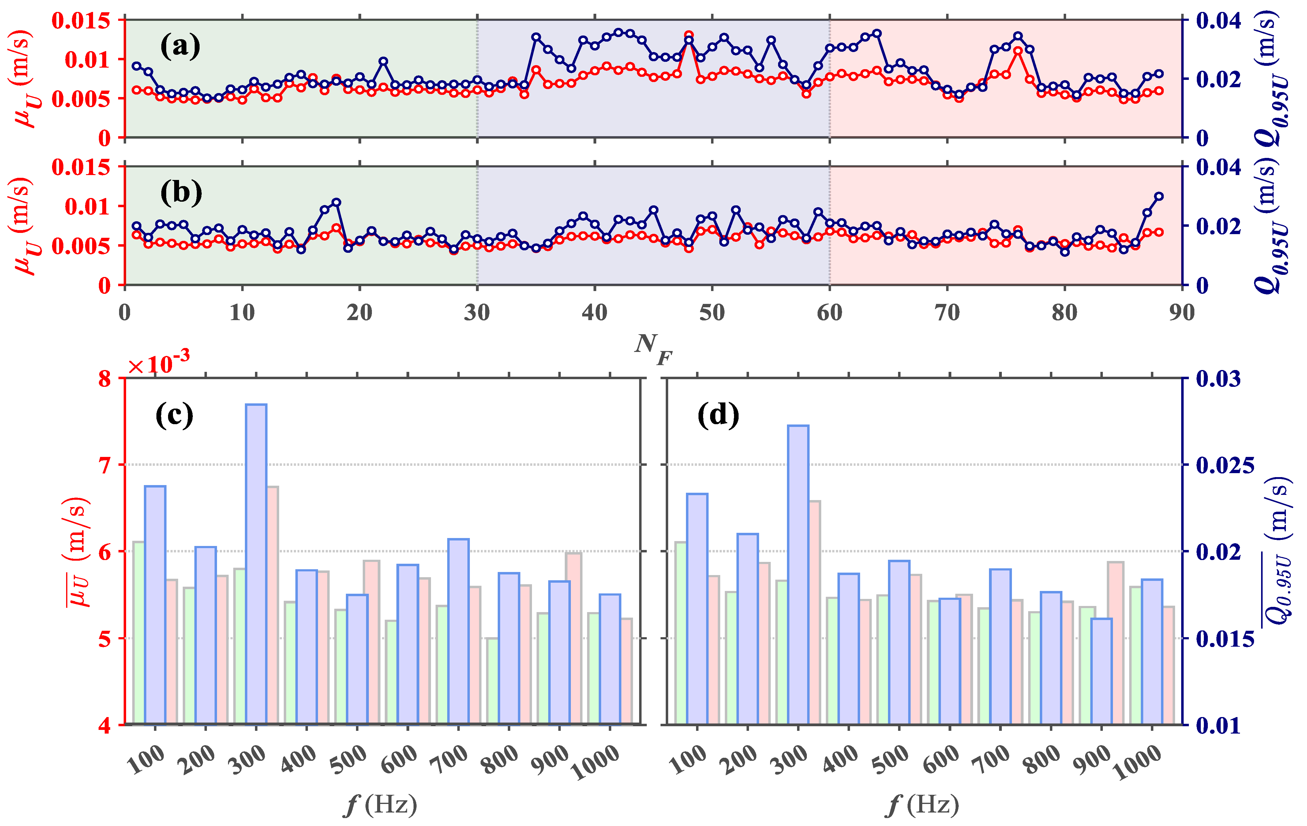
Figure 2a,b presents time-series of two velocity statistics, and , before (frames 1–29), during (frames 30–59), and after the tone (frames 60–89). Figure 2a corresponds to a 300 Hz tone, which shows variation after the tone frame with a sudden jump in both mean and 95th percentile velocities. Figure 2b shows the 400 Hz tone, where bulk behaviors of larvae are comparatively less affected by the sound. Figure 2c,d compares mean and 95th percentile of velocities averaged over frames: (1) before the exposure to sound (1–29 frame), (2) during continuous sound (30–59 frame) and (3) after sound was ceased (60–89 frame) at each frequency condition ranging between 100 to 1000 Hz.
For most of the frequencies studied, we saw a sudden jump in velocities during the tone, which did not persist after the sound ceased (Figure 2c,d). The velocity increment at the tone frame varied by frequency. We saw a greater response for 300 Hz, and decreasing velocities after the tone as frequencies increase. To validate whether the small variations of bulk velocities at higher frequencies could be interpreted as a significant larval response to sound, we analyzed individual behavior of larva when exposed to 400 Hz acoustic signal, since bulk velocities are seemingly less affected at this frequency condition (Figure 2c,d).
We calculated instantaneous fluctuations for each identified larva to assess individual responses, provided by error-bars in Figure 3a. A time series of dimensionless velocities defined by Equation (5) corresponding to individual larva is investigated in Figure 3b,c, so that the response to sound can be identified for each individual. Each larva is identified by a specific number, termed as larvae ID in Figure 3.
An example of this analysis is shown in Figure 3, for larvae exposed to a 400 Hz tone, which showed negligible variation of bulk velocities at the tone frame (as seen in Figure 2). Larvae were classified into two groups, those that showed an active response based on our 4 criteria (Figure 3b) and those that did not (Figure 3c). Looking at normalized velocities, we observe a clear distinction between before and after the tone frame (T = 30) as high normalized velocities with red colors appear mostly after the tone frame, in contrast with green, low velocities appearing before the tone. Such a change of behavior indicates that larvae included in Figure 3b were influenced by the tone, producing a change in displacement after the sound. On the other hand, high normalized velocities are observed at random frames in Figure 3c, regardless of the tone frame at T = 30. These irregular behaviors indicate that sound did not cause any noticeable change in motions for larvae that are included in Figure 3c. Although bulk velocities remained consistent to sound of 400 Hz in Figure 2b, 24% of larvae were still experiencing abrupt movements after the exposure to sound, as manifested by an increase in individual velocity.
3.2. Analysis Based on Individual Behavior of Larvae in Response to Sound Stimuli
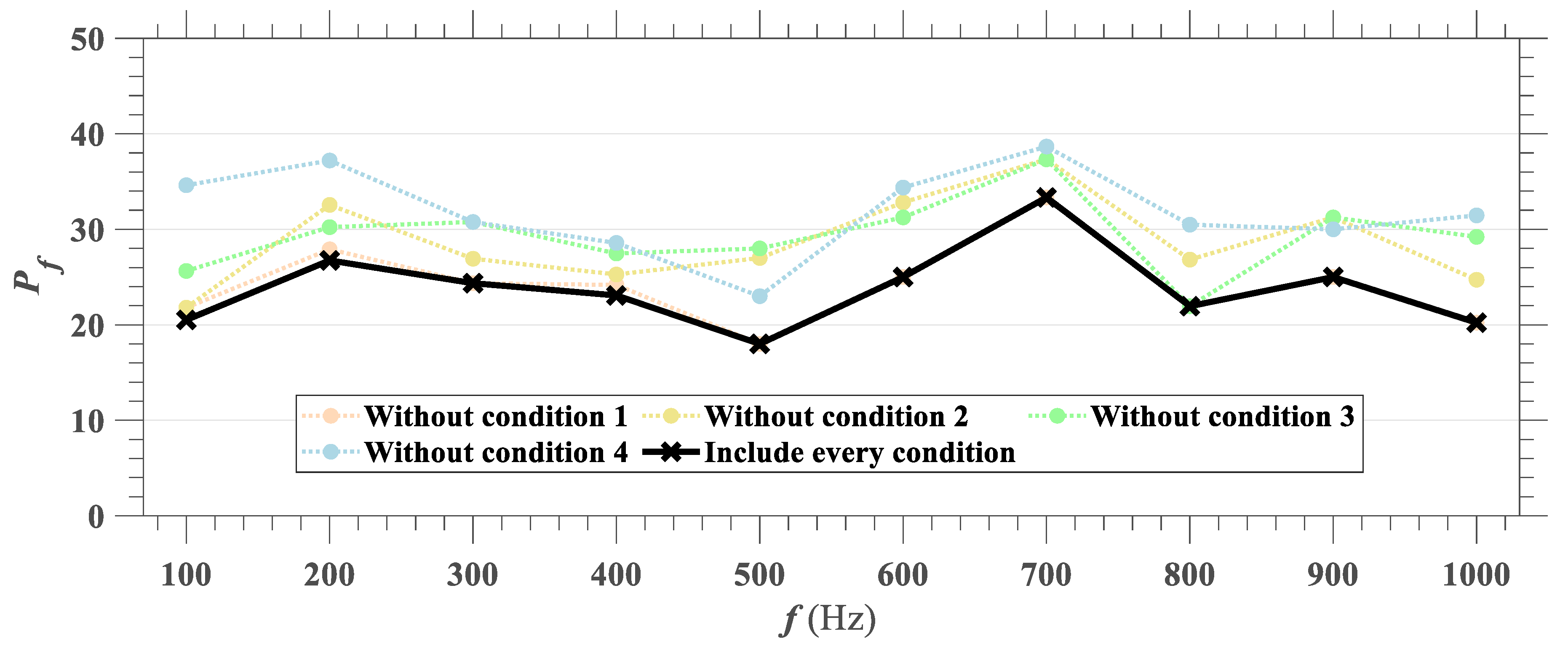
The solid black line in Figure 4 shows the response ratio over the frequency range of 100–1000 Hz. The lowest response ratio was computed at the sound of 500 Hz, with a comparatively smaller percentage of larvae changing their movement patterns after the tone, while 700 Hz seems the most effective to provoke a response in larvae, causing one third of them to experience a sudden jump in velocity at the tone frame.
In order to examine the sensitivity of response ratio to our four conditions to define larval response, we computed the ratio neglecting one condition, such that only the other three conditions had to be satisfied to consider an active response. Under this relaxed condition, response ratio ranged between 20–40%, slightly broader than the ratio computed with all four conditions being satisfied. Dotted lines in Figure 4 correspond to cases when one of the conditions was neglected, showing that results were almost consistent regardless of the combination of our established conditions. Thus, we can conclude that each condition had an equivalent contribution to define larval response, and all four conditions should be considered as our definition of an active response.
In Table 1, we provide the actual numbers of detected larvae, denoted as , along with numbers of larvae identified as having an active response, , for all frequencies. As the number of detected larvae were large enough to capture the wide range of behaviors at every frequency condition, we find our response ratio sufficient to analyze the extent of larval response to sound stimuli.
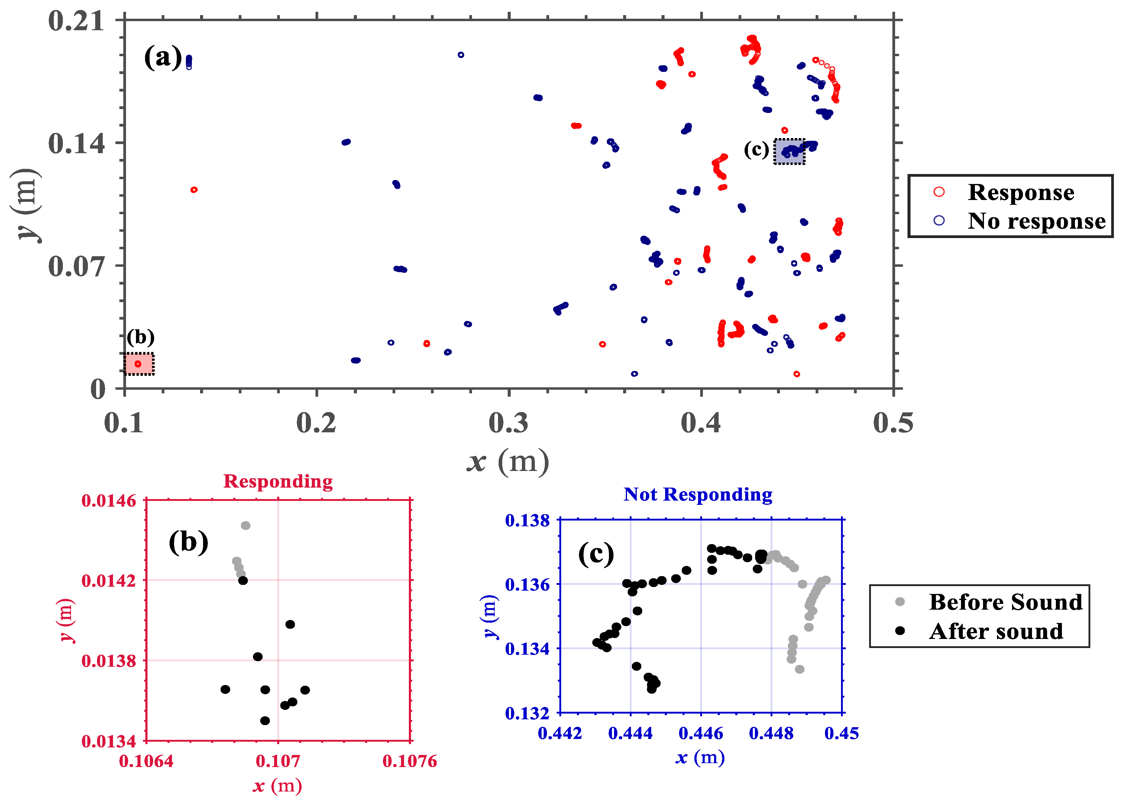
The distribution of every larvae located inside the fish tank and their trajectories during the experiment which lasted for 3 s are presented in below Figure 5 to provide an overview of larval movements. Figure 5 is obtained from larvae that are exposed to sound of 700 Hz while similar patterns are observed from experiments with other frequency ranges as well.
Since the magnitude of displacement and length of trajectories vary by individual, few larvae might seem static, although they are defined as responding to sound with an abrupt initiation of motion at the tone frame. Figure 5b focuses on one of those larvae and provides its trajectory to show that the larva changed the motion at the tone frame although it is not visible in Figure 5a. On the other side, if a larva is constantly moving, even before the tone, as depicted in Figure 5c, the larva would be defined as not responding to sound, even when evident displacements are observed in Figure 5a, since no significant change occurred at the tone. We must note that the accumulation of larvae near wall regions in Figure 6a is not because larvae were more sensitive to sound at specific locations, but rather because they were initially concentrated there from the beginning of the study.
4. Discussion
4.1. Analysis Based on Bulk Behavior of Larvae in Response to Sound Stimuli: Possibilities of Misrepresenting Individual Larval Behaviors
The analysis based on bulk quantifications of larval velocity could lead to conclusions that: (a) grass carp larvae can perceive tones in the range of 100–1000 Hz; (b) tones with frequency of 300 Hz could exert a more significant response in grass carp larvae; and (c) increasing frequencies past 300 Hz will not produce significant responses. However, large fluctuations in velocities among individual larva (Figure 3a, with vertical error-bars representing variance of larval velocity), hints at misrepresentations of carp behavior using only a mean value. The large disparity of velocity trend between responding and non-responding larvae (Figure 3b,c) demonstrates that bulk velocities are not sufficient to quantify the response of larvae to sound, since behaviors vary by individual. Although the larvae were exposed to identical acoustic stimuli at the same time, high velocities (marked by red dots in Figure 3b) are concentrated right after the tone frame for larvae that are responding to sound, while high velocities (red dots in Figure 3c) and low velocities (green dots in Figure 3c) are randomly distributed for larvae that are not responding to sound. Thus, we suggest that number of individual larvae reacting to sound should be counted, and its ratio should be used to better quantify the extent of larvae response to sound stimuli.
4.2. Analysis Based on Individual Behavior of Larvae in Response to Sound Stimuli: Methodology Considerations to Improve Assessment of Larval Response
The most conspicuous difference between analysis based on bulk behaviors (i.e., quantification with mean and 95th percentile velocities) and individual behavior (i.e., quantification with response ratio) is whether carp larvae are reacting more actively at certain frequency ranges of sound. From the perspective of individual larval response, we didn’t observe any clear relation between frequency and response ratio, but rather a consistent proportion of larvae were reacting to sound stimuli, with response ratio ranging between 20–30% regardless of the frequency.
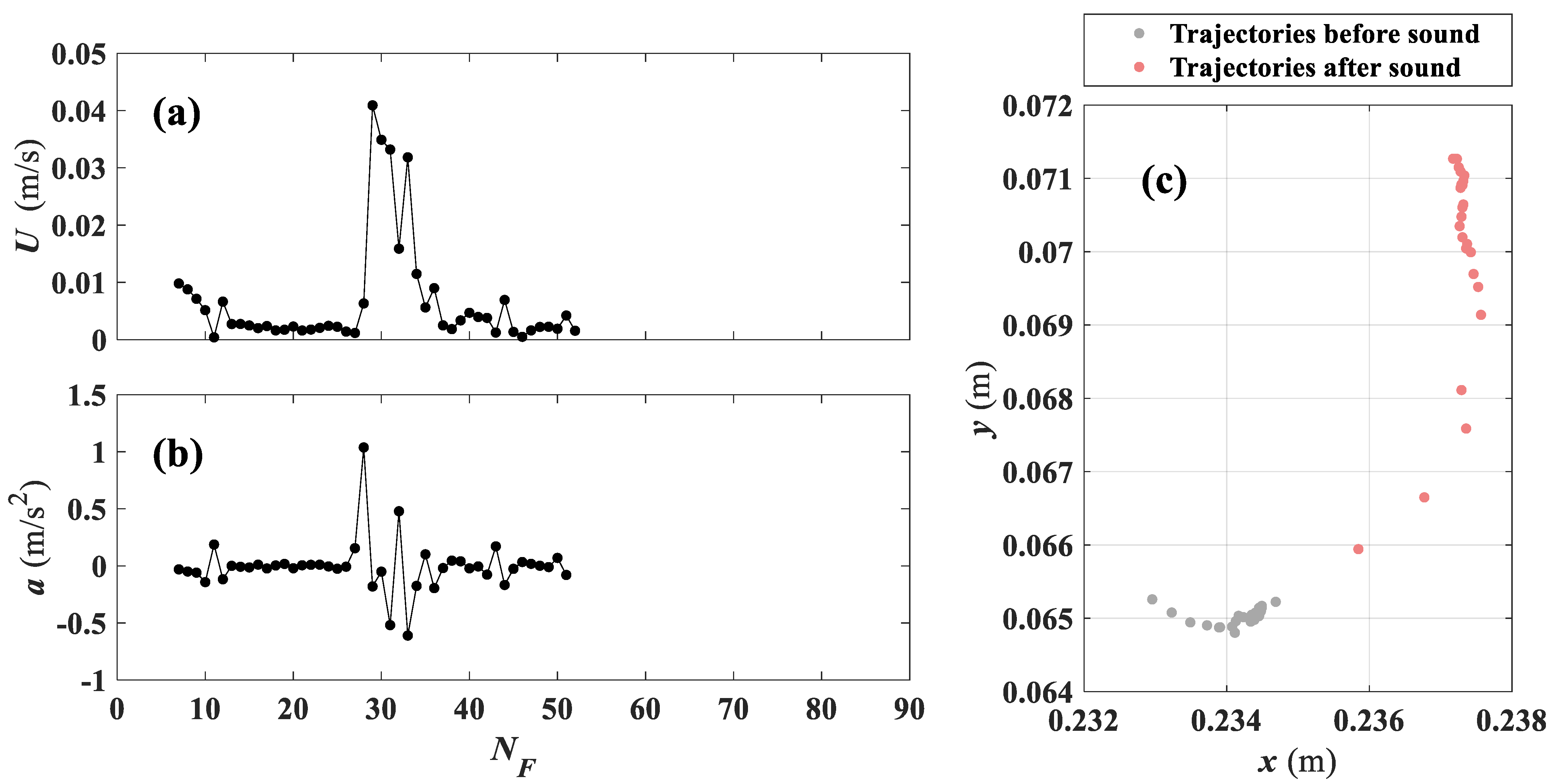
Looking at the individual response, time-series of velocity and acceleration for a single larva (Figure 6), these show a clear change near the tone frame, for a larva responding to the tone. In Figure 6a,b, velocities and accelerations are close to zero before the tone, which shows that movements of larvae were negligible. At the moment of exposure to sound, velocity jumps to a peak value and active larvae movements are maintained for a short period of time. A large fluctuation in acceleration is also observed at the tone. Trajectories of larvae in Figure 6c also confirm the larval response to sound, as the distance between instantaneous position on each frame reaches a maximum right after larvae were exposed to sound (i.e., even if larvae were already moving prior to the tone, which would report a pre-existing velocity prior to the stimulus, they clearly accelerate when they perceive the sound). Thus, trajectories and time-series of velocity and acceleration are appropriate indices of larval response to sound which are considered to compute response ratio in this study.
The duration of the response varied within individuals. The larva shown in Figure 6, for example, had a comparatively short duration of response, lasting only 4–5 frames. In general, the response lasted shorter than a second and died out before the sound ceased. Although we provide data from one typical larva in Figure 6, peak velocities, acceleration observed near the tone frame, and larger displacements right after the sound were common behaviors among larvae that responded to sound.
As large number of larvae were exposed to sound at the same time, the interaction between neighboring larvae to generate additional motions were also observed. It is shown from Figure 5 that the movement of each larva was independent from one another, and sudden initiation of motion among neighbors did not startle nearby larvae to start their motions as well. Thus, we concluded that sudden change in motion at the tone purely results from each larva acknowledging the sound, and their decision on how to react to that stimulus.
4.3. Limitations and Applications of Current Research
Several limitations remain in this type of studies, which requires future tasks to design effective sound barriers. Our experiment was designed to test larvae response to acoustic stimuli at still water condition while the actual habitat of carp larvae would be flowing rivers. Thus, we expect higher variability among larval responses to sound in the fields. Due to short duration of sound in our experiment, the consistency of larvae response was not considered, while carps’ fast adaptation to acoustic stimuli has been recently raised as a concern when implementing sound barriers [19]. In addition, we only analyzed the response of larvae at pure tones whereas previous studies reported various effective designs of acoustic barriers such as exposing mixed tones and combining acoustic stimuli with other types of barrier [2,20].
No type of sensory deterrent systems can be 100% effective but different combinations of deterrents can provide an effective solution for expansion of invasive carp species in Midwest Rivers. Although the response ratio was comparatively moderate, our study showed that grass carp larvae can acknowledge acoustic signals, which suggests the applicability of sound to be used in a different combination of deterrents.
Although we only focused on the larval response to acoustic signal in this paper, efficacy of other types of deterrents can be also quantified based on similar framework of analysis based on PTV by tracking trajectories of larvae and analyzing the variation of velocities and acceleration when they are exposed to external stimuli. For actual application of deterrents in real rivers, field tests are required to consider the effect of diverse biotic and abiotic variables on the interaction between carps and deterrents. Our framework of analysis based on particle tracking velocimetry is advantageous in that it can be applied to both lab and field work since we only need the recordings of trajectories of carps to identify altered navigation due to external stimuli. We expect that the negative impact of invasive carps on freshwater ecosystem and surrounding morphodynamics can be alleviated by active future research on the efficacy of various deterrents, including acoustic stimuli, with careful consideration of both bulk and individual behaviors based on our proposed framework.
5. Conclusions
Grass carp larvae demonstrated a consistent response ratio ranging between 20–30% when exposed to acoustic signals of pure tones ranging from 100 to 1000 Hz. Maximum response ratio was calculated as 33% at 700 Hz, although we did not observe any clear relation between frequency and response ratio. This result differs from our observations based on mean bulk velocities, which showed a larger response at a 300 Hz tone. Sharply increased velocities at the tone frame did not last long, and larvae returned to the original inactive state even before the sound ceased. Larvae were also insensitive to movements of neighbors which indicates that sudden motions at the tone frame were caused purely as a reaction to the acoustic signal.
The most significant finding in this study is that bulk quantification of larval motion can misrepresent their actual sensitivity and response to acoustic signal. Analysis based on bulk velocities indicate that larvae are sensitive to sound of low frequencies while in fact, larval response was not prominent at any specific frequency ranges when analyzed based on individual trajectories. Consistent response ratio implies that several larvae were startled by sound even when bulk velocity increased negligibly at the tone frame. High standard deviation of velocities is another indicator to suggest that larval response to acoustic signals is highly dependent on the behavior of each individual larva. Our result points out that quantifications of an optimal or threshold frequency to alter grass carp behavior depend on how the ‘response’ is defined. High deviation among individual behaviors highlights that it is necessary to simultaneously test a sufficient number of carp rather than repeating the experiment with a limited number of individual specimens, which will help us determine the general sensitivity and overall response to acoustic signals.
Author Contributions
H.Y. actively participated in data analysis and in manuscript preparation; R.O.T. participated with experimental design, assisted with data analysis and edited manuscript. All authors have read and agreed to the published version of the manuscript.
Funding
H.Y. was supported by Kwanjeong Educational Foundation.
Institutional Review Board Statement
The study was approved by the Illinois Department of Natural Resources and conducted according to their guidelines (Permit No. 18-050 issued 4/19/18). Larvae were euthanized prior to yolk sac absorption, such that no IACUC protocol was required.
Informed Consent Statement
Not applicable.
Data Availability Statement
The data presented in this study are available on request from the corresponding author. The data are not publicly available due to restrictions of animal use.
Acknowledgments
We thank A. Prada, A. George, and B. Stahlschmidt for transport and handling of the specimens used in the study.
Conflicts of Interest
The authors declare no conflict of interest.
References
- Mitchell, A.J.; Kelly, A.M. The public sector role in the establishment of grass carp in the United States. Fisheries 2006, 31, 113–121. [Google Scholar] [CrossRef]
- Dennis, C.E.; Zielinski, D.; Sorensen, P.W. A complex sound coupled with an air curtain blocks invasive carp passage without habituation in a laboratory flume. Biol. Invasions 2019, 21, 2837–2855. [Google Scholar] [CrossRef]
- Noatch, M.R.; Suski, C.D. Non-physical barriers to deter fish movements. Environ. Rev. 2012, 20, 71–82. [Google Scholar] [CrossRef]
- Zielinski, D.P.; Sorensen, P.W. Silver, bighead, and common carp orient to acoustic particle motion when avoiding a complex sound. PLoS ONE 2017, 12, e0180110. [Google Scholar] [CrossRef] [PubMed] [Green Version]
- George, A.E.; Garcia, T.; Chapman, D.C. Comparison of size, terminal fall velocity, and density of bighead carp, silver carp, and grass carp eggs for use in drift modeling. Trans. Am. Fish. Soc. 2017, 146, 834–843. [Google Scholar] [CrossRef]
- Lovell, S.J.; Stone, S.F.; Fernandez, L. The economic impacts of aquatic invasive species: A review of the literature. Agric. Resour. Econ. Rev. 2006, 35, 195–208. [Google Scholar] [CrossRef]
- Vetter, B.J.; Murchy, K.A.; Cupp, A.R.; Amberg, J.J.; Gaikowski, M.P.; Mensinger, A.F. Acoustic deterrence of bighead carp (Hypophthalmichthys nobilis) to a broadband sound stimulus. J. Great Lakes Res. 2017, 43, 163–171. [Google Scholar] [CrossRef] [Green Version]
- Scholik, A.R.; Yan, H.Y. The effects of noise on the auditory sensitivity of the bluegill sunfish, Lepomis macrochirus. Comp. Biochem. Physiol. Part A Mol. Integr. Physiol. 2002, 133, 43–52. [Google Scholar] [CrossRef]
- Vetter, B.J.; Brey, M.K.; Mensinger, A.F. Reexamining the frequency range of hearing in silver (Hypophthalmichthys molitrix) and bighead (H. nobilis) carp. PLoS ONE 2018, 13, e0192561. [Google Scholar] [CrossRef] [PubMed]
- Popper, A.N. Pure-tone auditory thresholds for the carp, Cyprinis carpio. J. Acoust. Soc. Am. 1972, 52, 1714–1717. [Google Scholar] [CrossRef]
- Willis, D.J.; Hoyer, M.V.; Canfield Jr, D.E.; Lindberg, W.J. Training grass carp to respond to sound for potential lake management uses. N. Am. J. Fish. Manag. 2002, 22, 208–212. [Google Scholar] [CrossRef]
- Nissen, A.C.; Vetter, B.J.; Rogers, L.S.; Mensinger, A.F. Impacts of broadband sound on silver (Hypophthalmichthys molitrix) and bighead (H. nobilis) carp hearing thresholds determined using auditory evoked potential audiometry. Fish. Physiol. Biochem. 2019, 45, 1683–1695. [Google Scholar] [CrossRef] [PubMed]
- Wright, K.J.; Higgs, D.M.; Leis, J.M. Ontogenetic and interspecific variation in hearing ability in marine fish larvae. Mar. Ecol. Prog. Ser. 2011, 424, 1–13. [Google Scholar] [CrossRef] [Green Version]
- Prada, A.F.; George, A.E.; Stahlschmidt, B.H.; Jackson, P.R.; Chapman, D.C.; Tinoco, R.O. Influence of turbulence and in-stream structures on the transport and survival of grass carp eggs and larvae at various developmental stages. Aquat. Sci. 2020, 82, 16. [Google Scholar] [CrossRef] [Green Version]
- Tinoco, R.O.; Prada, A.F.; George, A.E.; Stahlschmidt, B.H.; Jackson, P.R.; Chapman, D.C. Identifying turbulence features hindering swimming capabilities of grass carp larvae (Ctenopharyngodon idella) through submerged vegetation. J. Ecohydraulics 2020, 1–13. [Google Scholar] [CrossRef]
- Brevis, W.; Niño, Y.; Jirka, G.H. Integrating cross-correlation and relaxation algorithms for particle tracking velocimetry. Exp. Fluids 2011, 50, 135–147. [Google Scholar] [CrossRef]
- Chilton, E.W.; Muoneke, M.I. Biology and management of grass carp (Ctenopharyngodon idella, Cyprinidae) for vegetation control: A North American perspective. Rev. Fish. Biol. Fish. 1992, 2, 283–320. [Google Scholar] [CrossRef]
- Prada, A.F.; George, A.E.; Stahlschmidt, B.H.; Chapman, D.C.; Tinoco, R.O. Survival and drifting patterns of grass carp eggs and larvae in response to interactions with flow and sediment in a laboratory flume. PLoS ONE 2018, 13, e0208326. [Google Scholar] [CrossRef] [PubMed] [Green Version]
- Vetter, B.J.; Cupp, A.R.; Fredricks, K.T.; Gaikowski, M.P.; Mensinger, A.F. Acoustical deterrence of silver carp (Hypophthalmichthys molitrix). Biol. Invasions 2015, 17, 3383–3392. [Google Scholar] [CrossRef]
- Murchy, K.A.; Cupp, A.R.; Amberg, J.J.; Vetter, B.J.; Fredricks, K.T.; Gaikowski, M.P.; Mensinger, A.F. Potential implications of acoustic stimuli as a non-physical barrier to silver carp and bighead carp. Fish. Manag. Ecol. 2017, 24, 208–216. [Google Scholar] [CrossRef]
Figure 1.
Detected larvae in a single frame. Red squares show detected larvae while yellow cross show mis-detected sediments from the particle-tracking velocimetry (PTV) algorithm.
Figure 1.
Detected larvae in a single frame. Red squares show detected larvae while yellow cross show mis-detected sediments from the particle-tracking velocimetry (PTV) algorithm.

Figure 2.
Statistics of larvae velocity in response to sound stimuli. Time series plot of ![Water 13 00603 i001]() : mean and
: mean and ![Water 13 00603 i002]() : 95th percentile at (a) f = 300 Hz and (b) f = 400 Hz where f is the frequency. Bar plot of (c) time averaged mean velocity and (d) time averaged 95 percentile velocity computed for
: 95th percentile at (a) f = 300 Hz and (b) f = 400 Hz where f is the frequency. Bar plot of (c) time averaged mean velocity and (d) time averaged 95 percentile velocity computed for ![Water 13 00603 i003]() : frames 1–29 (before sound tone),
: frames 1–29 (before sound tone), ![Water 13 00603 i004]() : frames 30–59 (during sound tone) and
: frames 30–59 (during sound tone) and ![Water 13 00603 i005]() : frames 60–89 (after sound tone ceased).
: frames 60–89 (after sound tone ceased).
 : mean and
  : 95th percentile at (a) f = 300 Hz and (b) f = 400 Hz where f is the frequency. Bar plot of (c) time averaged mean velocity and (d) time averaged 95 percentile velocity computed for
  : frames 1–29 (before sound tone),
  : frames 30–59 (during sound tone) and
  : frames 60–89 (after sound tone ceased).
Figure 2.
Statistics of larvae velocity in response to sound stimuli. Time series plot of ![Water 13 00603 i001]() : mean and
: mean and ![Water 13 00603 i002]() : 95th percentile at (a) f = 300 Hz and (b) f = 400 Hz where f is the frequency. Bar plot of (c) time averaged mean velocity and (d) time averaged 95 percentile velocity computed for
: 95th percentile at (a) f = 300 Hz and (b) f = 400 Hz where f is the frequency. Bar plot of (c) time averaged mean velocity and (d) time averaged 95 percentile velocity computed for ![Water 13 00603 i003]() : frames 1–29 (before sound tone),
: frames 1–29 (before sound tone), ![Water 13 00603 i004]() : frames 30–59 (during sound tone) and
: frames 30–59 (during sound tone) and ![Water 13 00603 i005]() : frames 60–89 (after sound tone ceased).
: frames 60–89 (after sound tone ceased).
: mean and : 95th percentile at (a) f = 300 Hz and (b) f = 400 Hz where f is the frequency. Bar plot of (c) time averaged mean velocity and (d) time averaged 95 percentile velocity computed for : frames 1–29 (before sound tone), : frames 30–59 (during sound tone) and : frames 60–89 (after sound tone ceased).
Figure 3.
Time series of (a) bulk velocity with vertical error bars representing velocity variance, (b) normalized velocities of individual larvae that responded to sound stimuli (c) normalized velocities of individual larvae that did not respond to sound stimuli. Data shown for the 400 Hz tone, which showed the lowest variation of bulk velocities after the tone frame in Figure 2.

Figure 4.
Ratio of larvae responding to sound stimuli for frequency range between 100–1000 Hz for different combinations of four conditions established to define larval response. Correlation coefficients (r) between response ratio satisfying four conditions and three conditions (excluding each condition respectively) was computed as = 0.98, = 0.77, = 0.65 and = 0.64, where the lower letter indicates which condition was excluded.

Figure 5.
(a) Spatial distribution of larvae showing a response to sound and their trajectories over 90 frames. Sub-domains inside the Figure 5a that are marked with transparent red and blue colors are zoomed-in at beneath (b) and (c) respectively. (b) Example of larvae with subtle movements, but defined as having response to sound stimuli. (c) Example of larvae constantly moving throughout the entire time frame and thus defined as having no response to sound stimuli. The figure was obtained for larvae exposed to sound of 700 Hz, which led to the highest response ratio among larvae.

Figure 6.
Time series of (a) velocity and (b) acceleration to illustrate characteristics of larvae identified as actively responding to sound stimuli. (c) Trajectory of larvae obtained from the particle tracking algorithm. Data were obtained from 600 Hz tone.
Figure 6.
Time series of (a) velocity and (b) acceleration to illustrate characteristics of larvae identified as actively responding to sound stimuli. (c) Trajectory of larvae obtained from the particle tracking algorithm. Data were obtained from 600 Hz tone.


Table 1.
Number of larvae that were detected by PTV algorithms and defined as having response to sound stimuli.
Table 1.
Number of larvae that were detected by PTV algorithms and defined as having response to sound stimuli.
| f (Hz) | |||
|---|---|---|---|
| 100 | 78 | 16 | 20.51 |
| 200 | 86 | 23 | 26.74 |
| 300 | 78 | 19 | 24.36 |
| 400 | 91 | 21 | 23.08 |
| 500 | 100 | 18 | 18.00 |
| 600 | 64 | 16 | 25.00 |
| 700 | 75 | 25 | 33.33 |
| 800 | 82 | 18 | 21.95 |
| 900 | 89 | 20 | 25.00 |
| 1000 | 89 | 18 | 20.22 |
Publisher’s Note: MDPI stays neutral with regard to jurisdictional claims in published maps and institutional affiliations. |
© 2021 by the authors. Licensee MDPI, Basel, Switzerland. This article is an open access article distributed under the terms and conditions of the Creative Commons Attribution (CC BY) license (http://creativecommons.org/licenses/by/4.0/).
Share and Cite
MDPI and ACS Style
You, H.; Tinoco, R.O. Quantifying the Response of Grass Carp Larvae to Acoustic Stimuli Using Particle-Tracking Velocimetry. Water 2021, 13, 603. https://doi.org/10.3390/w13050603
AMA Style
You H, Tinoco RO. Quantifying the Response of Grass Carp Larvae to Acoustic Stimuli Using Particle-Tracking Velocimetry. Water. 2021; 13(5):603. https://doi.org/10.3390/w13050603
Chicago/Turabian StyleYou, Hojung, and Rafael O. Tinoco. 2021. "Quantifying the Response of Grass Carp Larvae to Acoustic Stimuli Using Particle-Tracking Velocimetry" Water 13, no. 5: 603. https://doi.org/10.3390/w13050603
Note that from the first issue of 2016, this journal uses article numbers instead of page numbers. See further details here.