
Water Pipe Replacement Scheduling Based on Life Cycle Cost Assessment and Optimization Algorithm


Department of Civil Engineering, Kyung Hee University, 1732 Deogyeong-daero, Giheung-gu, Yongin-si 17104, Korea
*
Author to whom correspondence should be addressed.
Water 2021, 13(5), 605; https://doi.org/10.3390/w13050605
Submission received: 3 February 2021
/
Revised: 15 February 2021
/
Accepted: 23 February 2021
/
Published: 25 February 2021
(This article belongs to the Special Issue Infrastructure Asset Management of Urban Water Systems)
Abstract
:Water distribution networks (WDNs) comprise a complex network of pipes and are crucial for providing potable water to urban communities. Therefore, WDNs must be carefully managed to avoid problems such as water contamination and service failures; however, this requires a large budget. Because WDN components have different statuses depending on their installation year, location, transmission pressure, and flow rate, it is difficult to plan the rehabilitation schedule within budgetary constraints. This study, therefore, proposes a new pipe replacement scheduling approach to smooth the investment time series based on a life cycle cost (LCC) assessment for a large-scale WDN. The proposed scheduling plan simultaneously considers both the annual budget limitation and the optimum expenditure on the useful life of pipes. A multi-objective optimization problem consisting of three decision-making objectives—minimum imposed LCC on the network, minimum standard deviation of annual investment, and minimum average age of the network—is thus solved using a nondominated sorting genetic algorithm to obtain an optimal plan. Three scenarios with different pipe replacement time spans and different annual budget constraints are considered accordingly. The results indicate that the proposed scheduling framework provides an efficient water pipe replacement scheduling plan with a smooth management budget.
1. Introduction
A water distribution network (WDN) comprises a complex network of underground pipes and plays a key role in delivering potable water to urban communities [1]. WDN is one of the most expensive components of the overall water infrastructure and directly impacts people’s quality of life and economic prosperity [2]. Unfortunately, water infrastructure managers worldwide are now facing the problem of aging pipes in WDNs, and limited historical data have hampered cost-efficient replacements. Furthermore, low budgets and underinvestment in water infrastructure over recent decades have led to the degradation of WDNs. Therefore, replacing, designing, and optimally managing WDNs is expected to be a significant social challenge in the 21st century [3]. Pipelines age because of various internal and external factors that lead to a decrease in their functionality and an increase in their risk of failure; both of these issues can incur large social and economic costs [4]. Thus, pipeline rehabilitation must be scheduled effectively to ensure adequate water quality and structural performance [5]. In practice, suitable pipe replacement/rehabilitation requires a large budget. However, as noted above, budgets for rehabilitating water infrastructure are typically limited, thereby constraining the options available to water infrastructure managers. Thus, although water pipelines are aging, their replacement and rehabilitation rate is lagging. For a considerable proportion of WDN assets, an efficient and practical pipe replacement scheduling plan must satisfy the annual budget and minimize future costs while maintaining WDN functionality. Water infrastructure managers require sustainable, practical, and affordable solutions to address such issues. Over the last two decades, various methods have been developed to assist in WDN infrastructure management by determining the optimal replacement age based on deterioration failure, leakage, and breakage modeling coupled with additional parameters such as hydraulic capacity [6].
Since the 1960s, studies have developed both theoretical and practical WDN optimization methods. These include linear and nonlinear programming methods and heuristic, meta-heuristic, and hyper-heuristic search methods. Heuristic, meta-heuristic, and hyper-heuristic algorithms provide near-optimal solutions in the search space. However, the degree of deviation between near-optimal and real optimal solutions in these algorithms cannot be predicted. Nonetheless, these algorithms work well in dealing with large-scale systems and nonlinear relations in WDNs. For example, multi-objective optimization has been widely used in the design and rehabilitation of WDNs [7,8,9,10,11,12]. Further, as mentioned above, various optimization models have been applied to determine the optimal pipe replacement age while minimizing the economic cost [13,14,15,16], maximizing the system reliability, or both [17,18,19].
Alvisi and Franchini [17] used a multi-objective nondominated sorting genetic algorithm (NSGA-II) to predetermine budget constraints on WDN maintenance through optimal rehabilitation scheduling and leakage detection. Similarly, Nafi and Kleiner [20] proposed an approach to obtain an efficient pipe replacement schedule for a WDN subject to various budgetary constraints. Fuchs-Hanusch et al. [21] investigated the effect of pipe age on leakage and proposed a modified life cycle cost (LCC) equation that included leakage detection costs. Shin et al. [4] used a single-objective genetic algorithm to minimize the pipe replacement, renovation, and repair costs over a defined analysis period.
In particular, several researchers have applied the concept of LCC to WDNs. This powerful concept supports the analytical processes by which managers are able to make the most cost-effective decisions from among the options presented to them at different life cycle stages and that consequently have different costs [22]. In 1974, the US state of Florida adopted the LCC concept in the management of its WDN, and in 1975, the US Department of Health, Education, and Welfare initiated a project entitled “Life Cycle Budgeting and Costing as an Aid in Decision Making” [23].
Shamir and Howard [13] suggested an exponential relationship between the breakage rate and age of a pipe to determine the pipe replacement time at which the total repair and replacement cost is minimized; this is one of the basic ideas behind LCC. Lee et al. [24] developed an inventory method for the LCC analysis of a WDN by classifying each network item. This method was demonstrated to help water infrastructure managers determine when and which items in the WDN need to be rehabilitated. Marzouk and Osama [9] proposed a decision-making methodology to assist managers in their short- and long-term management plans. They considered four objective functions: The overall risk index, infrastructure condition, service level of an asset, and LCC. Further, they used a fuzzy Monte Carlo simulation to model the probability of failure. They found that economic parameters have the highest impact on assets’ consequences of failure, and pipe size has the highest impact on the overall consequence of failure index. Jayaram and Srinivasan [25] proposed a new multi-objective formulation to minimize the LCC and maximize network performance. Roshani and Filion [26] developed the OptiNET model to optimize the replacement time and pipe diameter to minimize the LCC. They determined the optimal replacement age by using capital and operational costs as the objective function. Frangopol and Soliman [27] noted that LCC analysis could significantly reduce long-term costs and increase infrastructure sustainability and resilience. Godfrey and Hailemichael [28] concluded that piped water supplies are less expensive than point source supplies when capital expenditure and emergency water supply costs are considered in the LCC. Hasegawa et al. [29] used the concept of LCC to examine the feasibility of pipe diameter reduction in a WDN during depopulation.
Using LCC for pipe replacement scheduling has advantages and disadvantages. On the one hand, LCC provides a reliable scheduling plan; on the other hand, it causes the required investment to peak in some years when the number of pipes needing replacement exceeds the budget. Indeed, though water infrastructure governors need to start putting more effort and funding towards fixing the problem of aging pipes in WDNs, over the last decade, most studies have proposed scheduling plans without considering budget restrictions (i.e., expenditure ceilings). In this study, the LCC is therefore used to propose an economical replacement plan for individual pipes in a real large-scale WDN by considering annual budget restrictions to smooth the annual investment time series based on optimization models. This approach considers three objective functions: Imposed LCC minimization, annual investment smoothing, and network age minimization. To the best of our knowledge, no previous study has investigated the use of smoothing to avoid investment peaks by considering all individual assets. In the proposed plan, the replacement time is relaxed from peak years to off-peak years while maintaining WDN reliability. The proposed method can be used to schedule the rehabilitation of a wide range of WDN assets and can determine the optimum number of service years of an individual asset by considering the above-mentioned objective functions. Thus, this method can enable the development of a more realistic budget for WDN rehabilitation.
The remainder of this paper is structured as follows. Section 2 describes the proposed approach and its methodology. Section 3 presents the optimization results obtained under three different scenarios. Finally, Section 4 discusses the application of the proposed method and presents the conclusions of this study.
2. Methodology
2.1. Optimal Water Pipe Replacement Based on LCC Assessment
LCC is one of the most critical factors in cost-effective decision-making for a system [30]. The LCC evaluation was thus employed in this study to achieve optimal pipe replacement scheduling. The LCC of a pipe is simply defined as the sum of all costs incurred during its entire life span. In general, the LCC for each pipe attribute is therefore calculated as the sum of acquisition, maintenance, replacement, repair, and disposal costs. In this study, the LCC is calculated as
where CI is the initial cost ($/km/year), CR is the running cost ($/km/year), D is pipe diameter (mm), and t is pipe replacement interval (year). Here, the CI includes only the pipe replacement cost per year and the CR includes only the pipe repair cost per year. The CI is calculated using:
where CP is the pipe replacement cost ($/km).
The CR is the product of the repair cost and the average failure rate during the replacement interval, and is therefore expressed as
where Cr is the pipe repair cost ($/failure) referred from [31] and expressed by
and Fr is pipe failure rate (failure/km/year), which is dependent on the pipe diameter and pipe age (A). This study uses the failure rate obtained by [4] as follows:
Available records of historical failure data must be used to estimate the WDN failure rate. This failure rate was derived through nonlinear regression analysis using the Statistical Package for the Social Sciences (SPSS, v. 18) and the input model suggested by [16]. This input model explains the relationship between the failure rate and the pipe attributes (i.e., diameter and age).
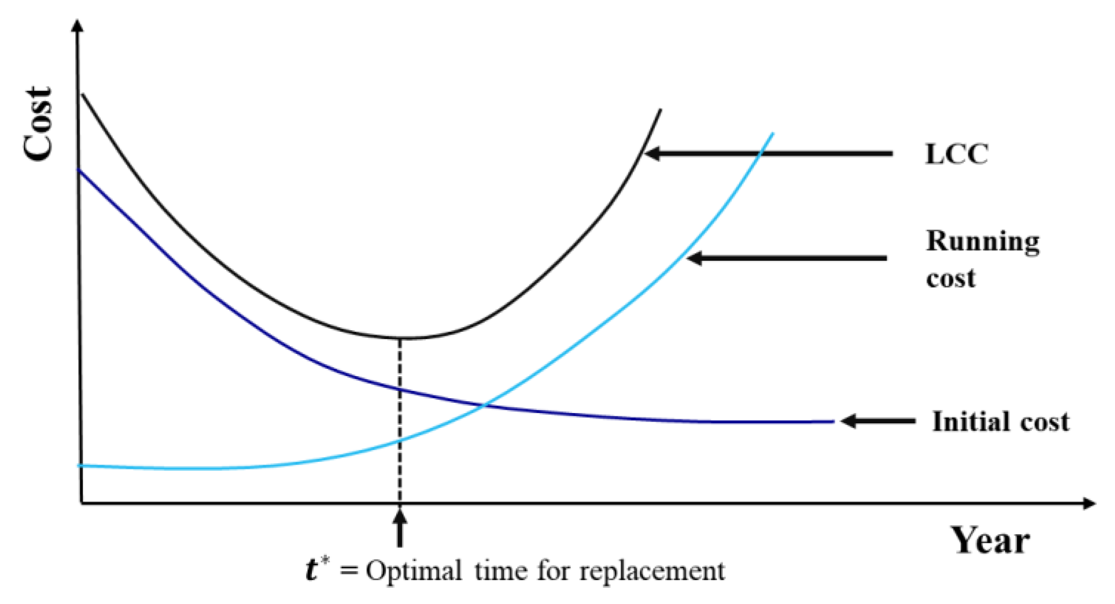
Figure 1 illustrates an example of an LCC curve, indicating that as the replacement age of a pipe increases, the running cost increases, and the initial cost decreases. The optimal time for replacement, or the most economic life span, is that for which the total cost is the minimum (), shown in Figure 1. In this study, the least life cycle cost (LLCC) for individual pipes is defined as the LCC at .
The summation of costs for all individual pipes at forms the LLCC of the network (LLCCN), which represents the cost at which the summation of the initial and running costs is the minimum, and is defined as
where n is the number of pipes in the network and Li is the length of pipe i.
The LCC for each pipe attribute (i.e., diameter and material) is calculated to determine the most economic replacement age for each individual pipe. However, to smooth the annual investment time series, the replacement time of each pipe should be relaxed within a time window around the optimal point () as shown in Figure 2.
Notably, the LCC curve can help engineers and decision-makers choose an appropriate and economical replacement policy [32]. The advantage of using the LCC curve is that it approximates the optimal economic replacement age and shows the change in total cost around this optimal point. If the total cost curve is flat around the optimum, as shown in Figure 2, the engineer need not plan for the replacement to be performed precisely at the optimum age (), thus indicating some flexibility in the replacement scheduling plan. Therefore, as shown in Figure 2, performing the replacement within the feasible replacement time boundary of ± (bounded by the lower boundary (LB) and upper boundary (UB)) has no significant effect on the total cost. By contrast, if the LCC curve is not flat around the optimal point and changes sharply on both sides, the replacement should be performed as close to the optimal age as possible. Note that Figure 2 shows that a change in replacement time will lead to an increase in the LCC whether the replacement time is moved forward or backward; however, moving the replacement time will impact the overall system age (i.e., pipe age).
2.2. Smoothing the Investment Time Series
An emerging challenge worldwide is the need to replace the vast numbers and lengths of deteriorating pipes beneath streets, as most pipes are nearing the end of their useful lives. According to the LCC concept, pipe replacements accrue towards the end of the useful life of the pipes. The optimal economic replacement age is when the replacement cost becomes lower than the failure cost (i.e., costs of burst and leaks).
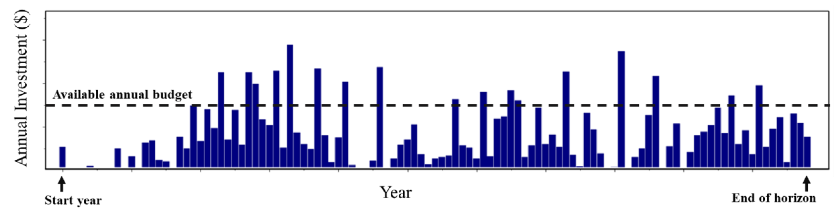
Based on the LCC formulation discussed in Section 2.1, the investment in each year () is the summation of the cost (CI and CR) of each pipe in a WDN; this leads to the formation of an investment time series. This investment time series imposes the minimum LCC on the network as well as the individual pipe if all pipes are replaced at their , which is determined based on the attribute (i.e., diameter and material) of each pipe. However, in some years, the required investment may exceed the annual budget, as shown in Figure 3, making the scheduling plan infeasible. To ensure that the scheduling plan remains feasible and close to actual practice, the investment time series needs to be smoothed to avoid investment peaks and meet the available annual budget. In order to do so, the investment time series needs to be changed so that investments in peak years are moved to off-peak years by changing the replacement time points for all individual pipes in the feasible replacement time boundary. The optimization algorithm (NSGA-II) was thus used in this study to obtain a set of replacement intervals for all pipes among those within the feasible replacement time boundary and smooth the investment time series as described in Section 2.3.
2.3. Pipe Replacement Scheduling Using a Multiobjective Optimization Algorithm
2.3.1. Overview of NSGA-II
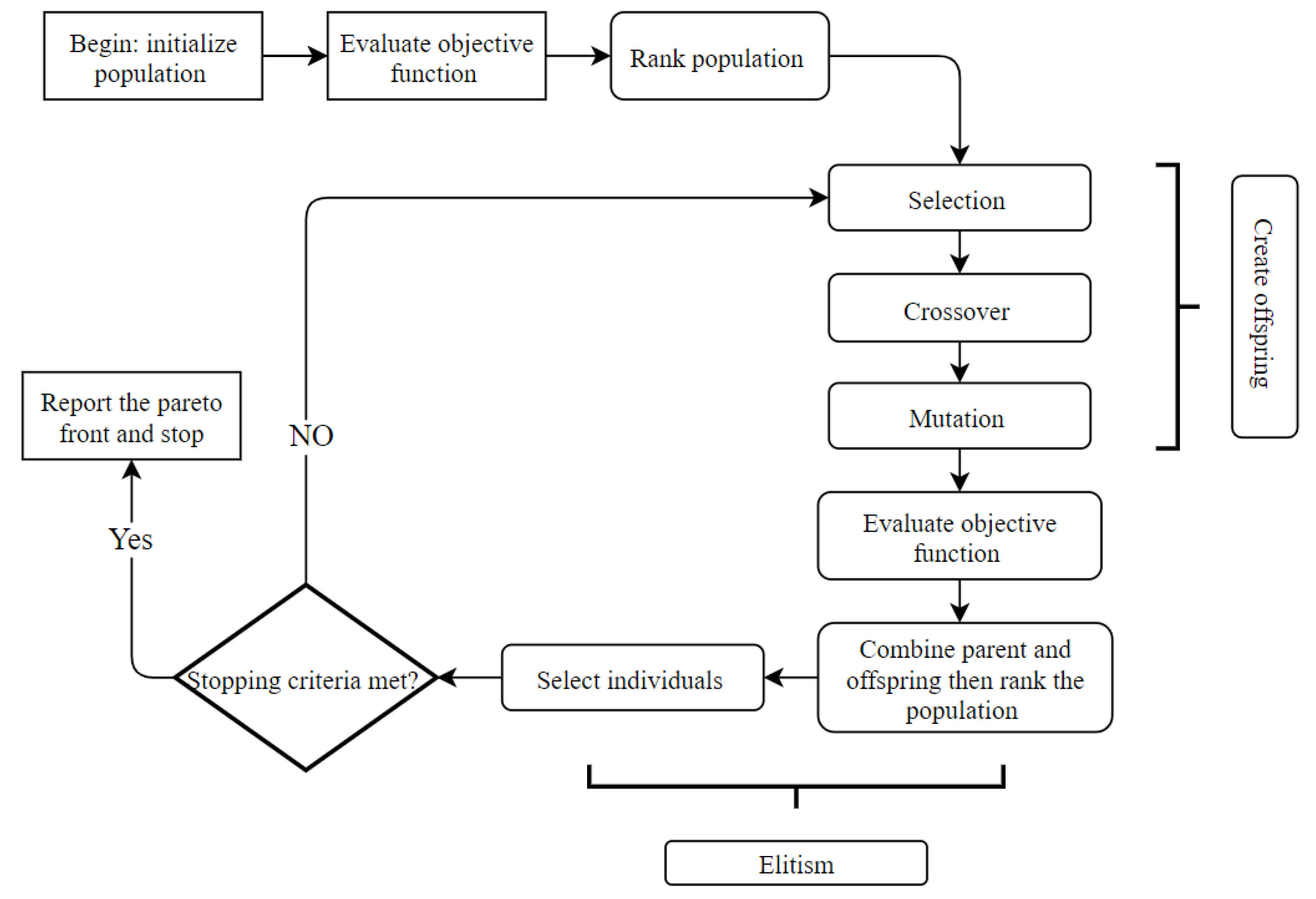
This study adopted the well-known and widely used multi-objective NSGA-II [33] as the optimization method. Figure 4 shows the optimization flowchart for NSGA-II and the general steps are briefly described below.
- NSGA-II randomly generates an initial population consisting of a number of chromosomes. Each chromosome is the value of the design parameter (i.e., the replacement time of an individual pipe).
- Each individual in the population generated in the previous step is ranked based on an evaluation of the objective function. Then, the individuals are sorted based on their rank by using the crowding distance.
- Parents are randomly selected from a mating pool to create the new generation. The mating pool consists of solutions with a higher crowding distance and rank.
- To produce offspring, parents from the previous step undergo crossover and mutation procedures. In the crossover procedure, two parents breed to produce an offspring that inherits its genes from both parents. In the mutation procedure, some values of the genes in each offspring are changed, thus providing the offspring with the opportunity to have at least one different gene value than their parents.
The previous steps are repeated until convergence is reached. In this study, the optimization algorithm was terminated after a defined number of generations. The efficiency of this algorithm can be improved by tuning its control parameters, such as the crossover and mutation rates, number of generations, and population size. To achieve the highest efficiency, various sets of control parameters were examined in this study.
2.3.2. Construction of Optimization Model
This study focused on developing a smooth, optimized replacement scheduling plan in which the peaks of investment time series are dispersed across a time span to meet the budget limit and use the available budget efficiently, while the LCC of each pipe in a WDN is kept as close as possible to its minimum value. The decision variable of the optimization model is a vector containing the optimal replacement time for all individual pipes, and the replacement time should be determined within a replacement time boundary ( ± ). The three objective functions of the problem are given by
where [·] represents the expectation operator, is a set of the annual investment, is the annual average age of pipes, and n is the number of pipes in the network. Equation (7) minimizes the imposed LCC of the network, that is, the difference between LCCN (i.e., LCC of the network) and LLCCN. By applying this objective function, the optimized LCCN is kept as close as possible to LLCCN, implying that the imposed cost is minimized. Equation (8) minimizes the standard deviation (SD) of the annual investments to smooth the investment time series. Equation (9) minimizes the average pipe age in the WDN to more reliably maintain the network [34].
The two main constraints considered in this study are the annual budget and the allowable replacement time interval ( ± ), during which the pipe replacement is performed. Considering the minimization of the three objective functions in Equations (7)–(9), the multi-objective optimization problem can be formulated as:
where is the available annual budget constraint (the total investment in each year must be equal or less than this value) and is the replacement time boundary.
3. Results
3.1. Case Study and Assumptions
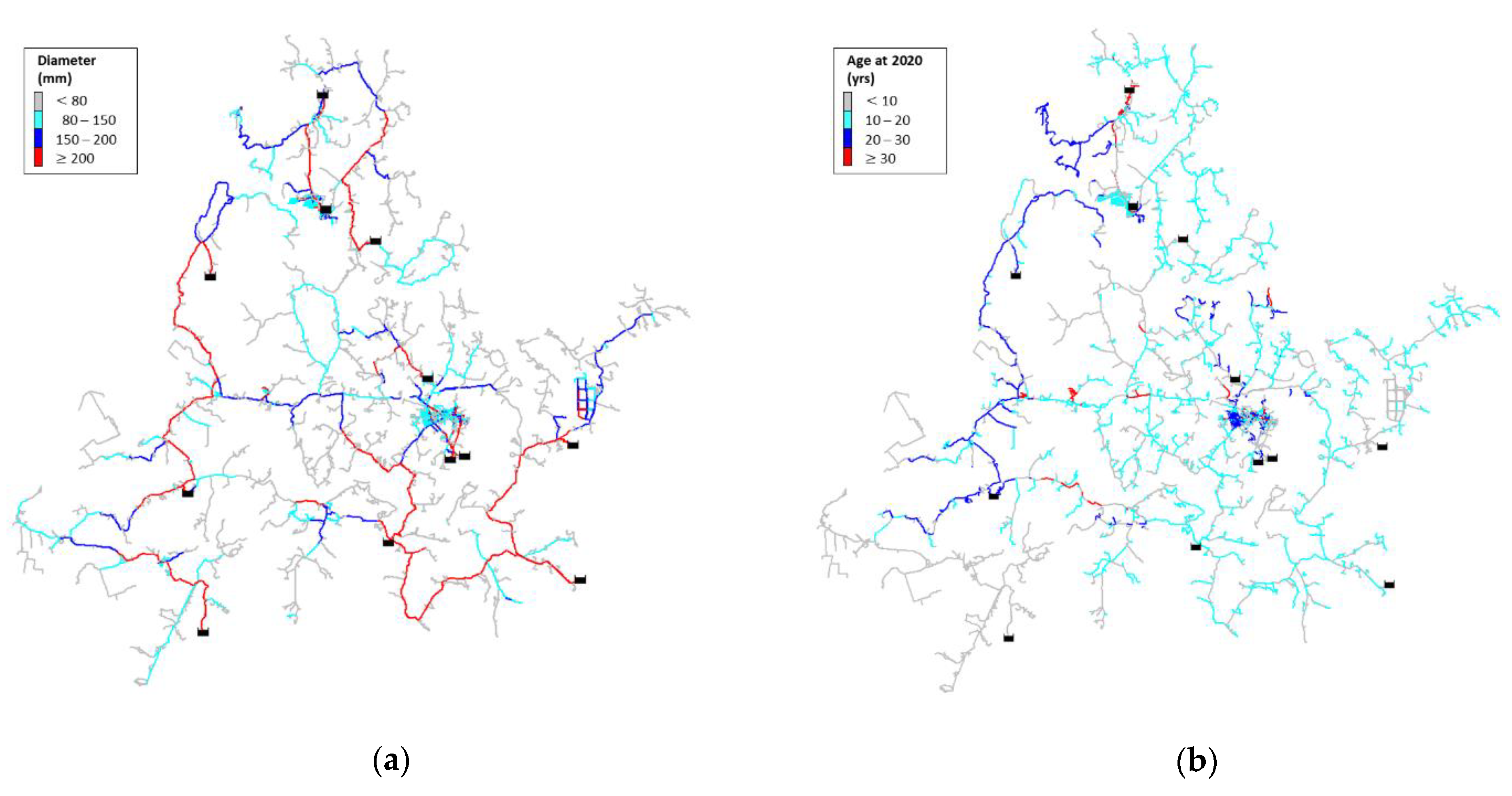
The proposed method was applied to a currently operating WDN in South Korea that consists of 6326 pipes with diameters ranging from 25–500 mm, as shown in Figure 5. Here, the total length of pipes is 812.5 km, and the percentages of pipe lengths in each diameter range are 57.4% (80 mm), 32.6% (80 mm 200 mm), 7.1% (200 mm 300 mm), 2.6% (300 mm 400 mm), and 0.3% (400 mm . In this study, only pipes with diameters of 80–500 mm were considered, which constituted 42.6% of the total length of all pipes and counted as 3042 pipes. Note that all pipes are made of the same material (i.e., ductile iron). The pipes can be divided into four groups according to their age in the year 2020, as shown in Figure 5b; 65.4% of the pipes are 10–20 years old.
It should be noted that the following assumptions were made in this case study:
- All pipes need to be replaced at least once in the simulation time horizon in consideration of the diameter and the first installation year of the pipes.
- Pipes that already passed their replacement time () will be replaced on priority in the first year of the scheduling plan.
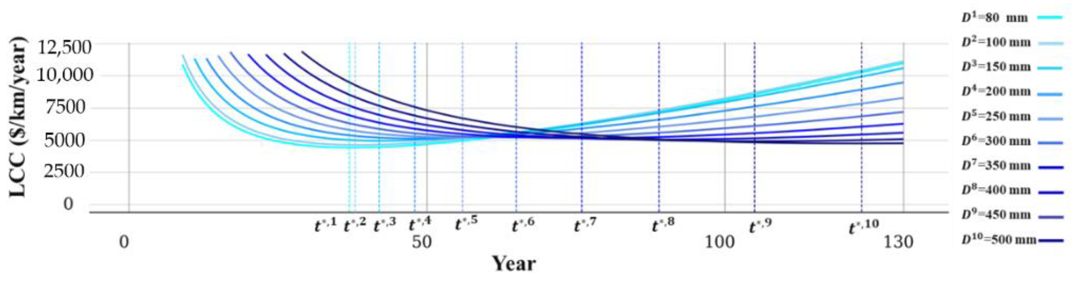
The initial costs of ductile iron pipe were obtained from the ‘Water Facilities Construction Cost Estimation Report’, published by K-water [35], and are summarized in Table 1. Table 2 shows the LLCC and corresponding for different pipe diameters. The LCC curves are shown in Figure 6, in which each color represents a different pipe diameter.
3.2. Pareto Front Obtained by Multiobjective Optimization
The NSGA-II was used to obtain the optimal replacement scheduling plan. The optimization model was developed in Python using the Pymoo library [36] and compiled with Cython 3 for parallel processing. For better convergence, the population size was set to 2000. The number of surviving offspring was set to 1500 to retain the best solutions in the population. Different generations were used for different scenarios in NSGA-II to obtain an extensive Pareto front and guarantee convergence. A simulated binary crossover function and a polynomial mutation operator with probabilities of 0.9 and 0.1, respectively, were used. The final run of the program with 2000 generations and population size of 2000 required approximately 99 h on an Intel® Core i9-10920X CPU @ 3.5 GHz with 128 GB memory. Three decision-making scenarios were considered during the optimization procedure as described below.
In the first scenario (Scenario 1), the feasible replacement time boundary () for changing the replacement time was set to 5 years, which means that the new replacement time could be in the interval of − 5 to + 5 years. The annual budget constraint was set to 2.5 M$ for the first scenario. In the second scenario (Scenario 2), the boundary was set to ± 10 years, and the annual budget constraint was 2.2 M$. In the third scenario (Scenario 3), the range was set to ± 16 years, and the annual budget constraint was 2.0 M$. The replacement time in all three scenarios lies within the LB and UB; this range was chosen based on the obtained LCC curve. As explained in Section 2.1, in the flat area of an LCC curve, the change in annual average cost is negligible, and the cost increases marginally when the replacement time is shifted to a different year to smooth the investment. Moreover, the chosen replacement time boundary depends on the budget constraint. Specifically, a wider time range (i.e., 16 years in the third scenario) leads to a smoother investment time series; by contrast, a narrower range (i.e., 5 years in the first scenario) leads to a small deviation from the LLCCN and, consequently, a less smooth investment time series that is likely to violate the budget constraint.
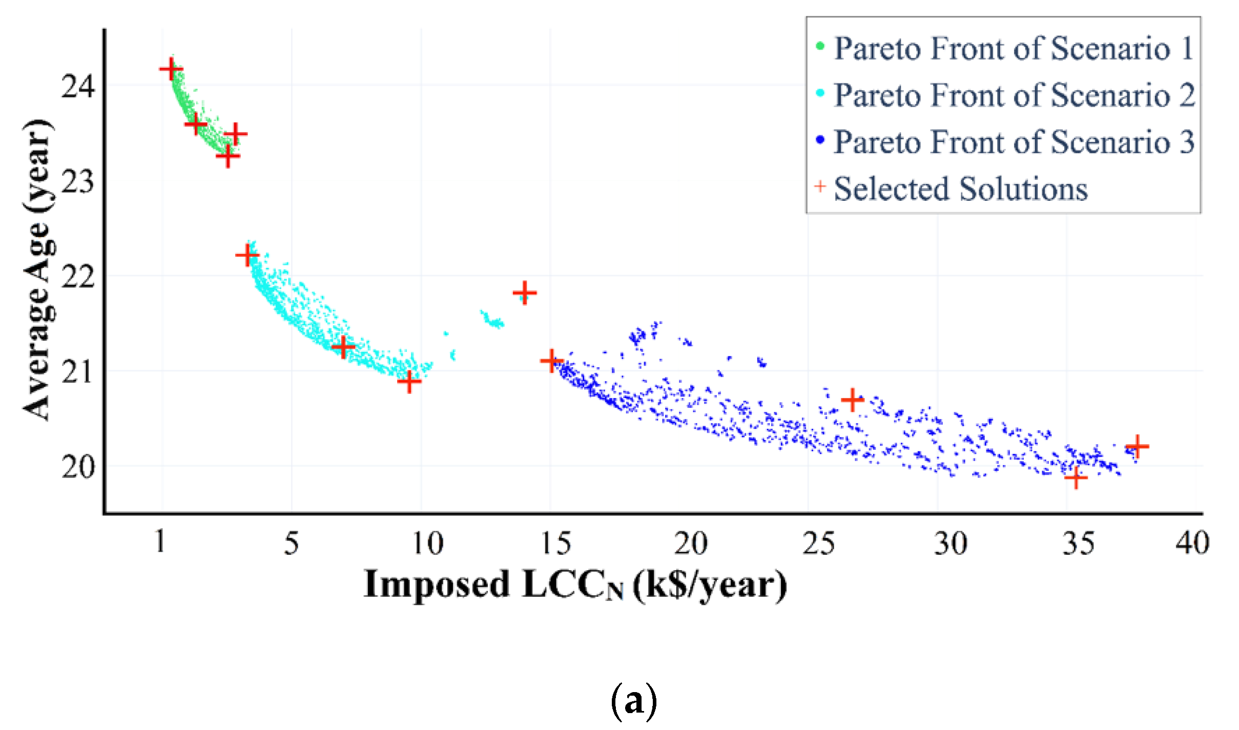
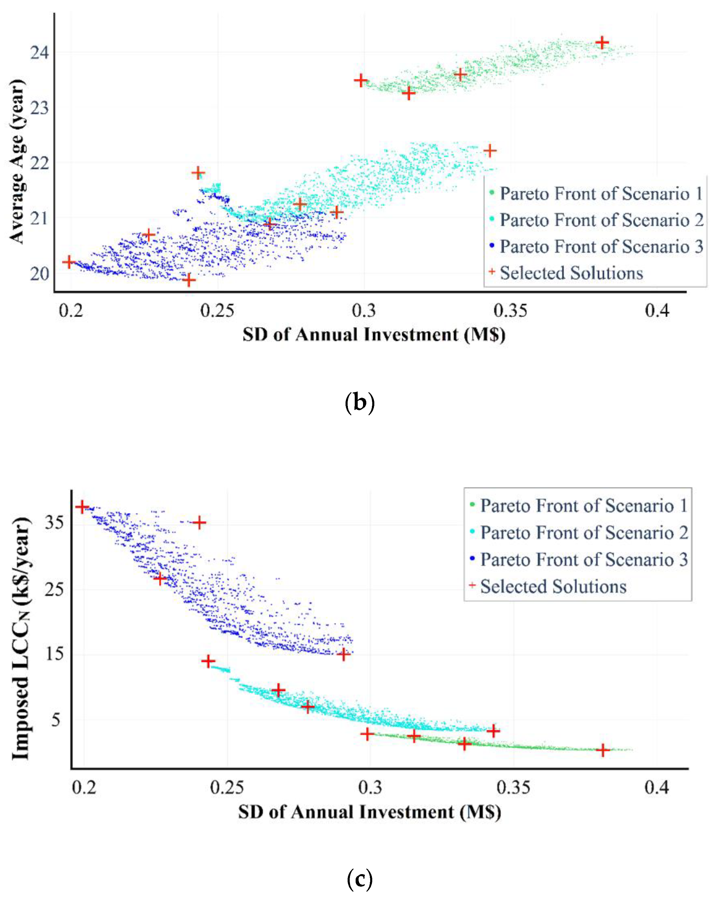
Figure 7 shows the nondominated Pareto solution obtained using NSGA-II for the three evaluated scenarios with different annual budget constraints and replacement time boundaries. The Pareto solutions of the first, second, and third scenarios are indicated in green, blue, and navy, respectively.
To analyze the characteristics of the optimal schedule, four representative solutions, including three corners and one knee-point, were selected from among all solutions for each of the three Pareto front scenarios, and are indicated by the red plus signs in Figure 7. The solutions at the three selected corners provided the minimum imposed LCC, minimum SD of annual investment, and minimum average WDN age among all solutions, and the knee-point provided the balanced solution for all three objectives. The knee-point was extracted after normalizing all three axes, after which it was the closest point to the origin. To increase the benefit of one of the three objectives, the other two objectives must clearly be sacrificed. Figure 7 shows the trade-off relationships among the three evaluated objectives.
To better clarify the relationship among these three objectives, the three-dimensional relationships in Figure 7 are projected in two-dimensional planes in Figure 8.
Referring to Figure 7 and Figure 8, it can be observed that the Pareto fronts resulting from this multi-objective pipe replacement scheduling problem indicate that a trade-off relationship exists among all three objectives, with the trade-off between the imposed LCC and SD of annual investment being the strongest, followed by that between the average WDN age and the imposed LCC. As the SD of the annual investment increases, the average WDN age increases and imposed LCC decreases, implying that the investment time series becomes less smooth, and the annual investment fluctuation increases. Comparing the Pareto fronts of all three scenarios, with an increasing replacement time boundary, the overall imposed LCC increases, but the average WDN age and variation of the annual investment decrease. Further, it can be observed that the Pareto front widens from Scenarios 1 to 3; as the replacement time boundary is more relaxed, the decision space increases, resulting in a larger number of alternative optimal solutions.
Comparing Scenarios 1 and 3 in Figure 7 and Figure 8, it can be seen that allowing the wider replacement time boundary and reducing the annual budget limit broadens the change in the imposed LCC, causing a wide variety of optimal solutions to appear in the Pareto front. In Scenario 1, which has the narrowest replacement time boundary and the highest annual budget, the replacement time does not change significantly from , thus LCC is minimum, but the annual variation and system age are the highest. Whereas in Scenario 3, which has the widest replacement time boundary and the lowest annual budget, the annual investment shows the smallest SD, implying that the investment time series is the smoothest. The results from all three scenarios indicate the presence of a trade-off relationship between the variation of the annual investment and the imposed LCC. A smoother investment time series leads to an increase in the imposed LCC, because the replacement is conducted sooner or later than .
3.3. Comparison of Solutions for WDN Investment
3.3.1. Future Investment Based on LLCCN
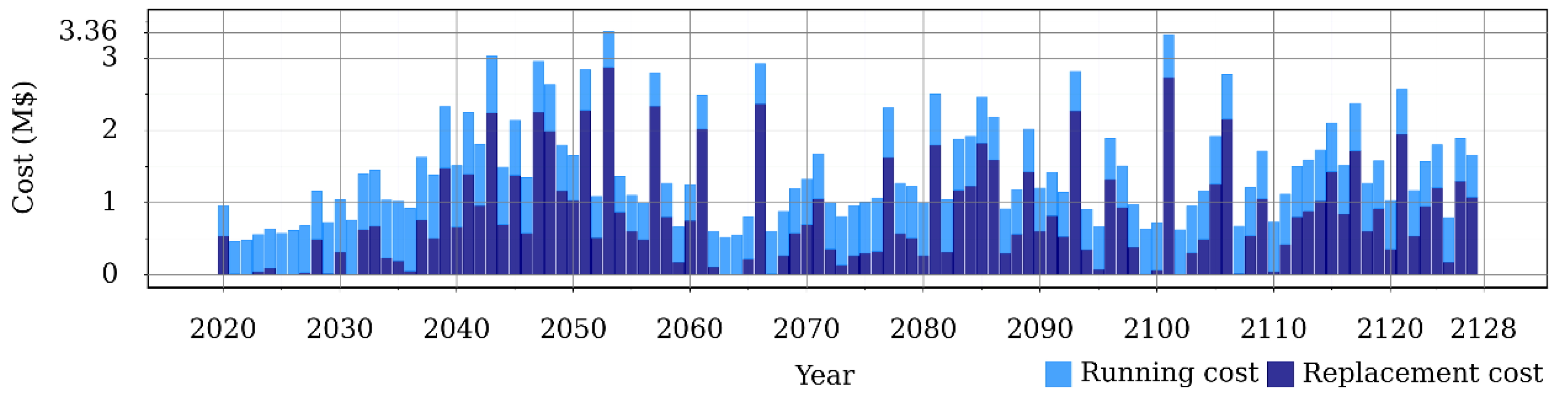
Figure 9 shows the investment time series for the WDN before smoothing. The value of investment for a specific year is calculated as the product of the replacement cost (initial cost) and the length of pipes replaced within that particular year; for the rest of the pipes, the investment value is calculated as the product of the running cost and the pipe length. In Figure 9, the replacement and running costs are indicated in navy and blue, respectively. In some years in Figure 9, a majority of pipes need to be replaced (e.g., 2053), and the share of replacement cost is high enough to jeopardize the replacement schedule. Moreover, there are some years in Figure 9 (e.g., 2026) in which no replacement is planned.
In these cases, moving items in the replacement queue from peak years to off-peak years will relieve budgetary pressure and lead to a reasonable and sensible replacement plan. In the next (Section 3.3.2, Section 3.3.3, Section 3.3.4), obtaining a smoother investment time series for the replacement schedule is explained in detail for the three scenarios. For a better comparison of the results in each of the three evaluated scenarios, details of the network before smoothing are shown in Table 3. Here, the total annual investment (TAI) is the total cost divided by the planning time horizon (i.e., 108 years).
3.3.2. Future Investment Based on Scenario 1
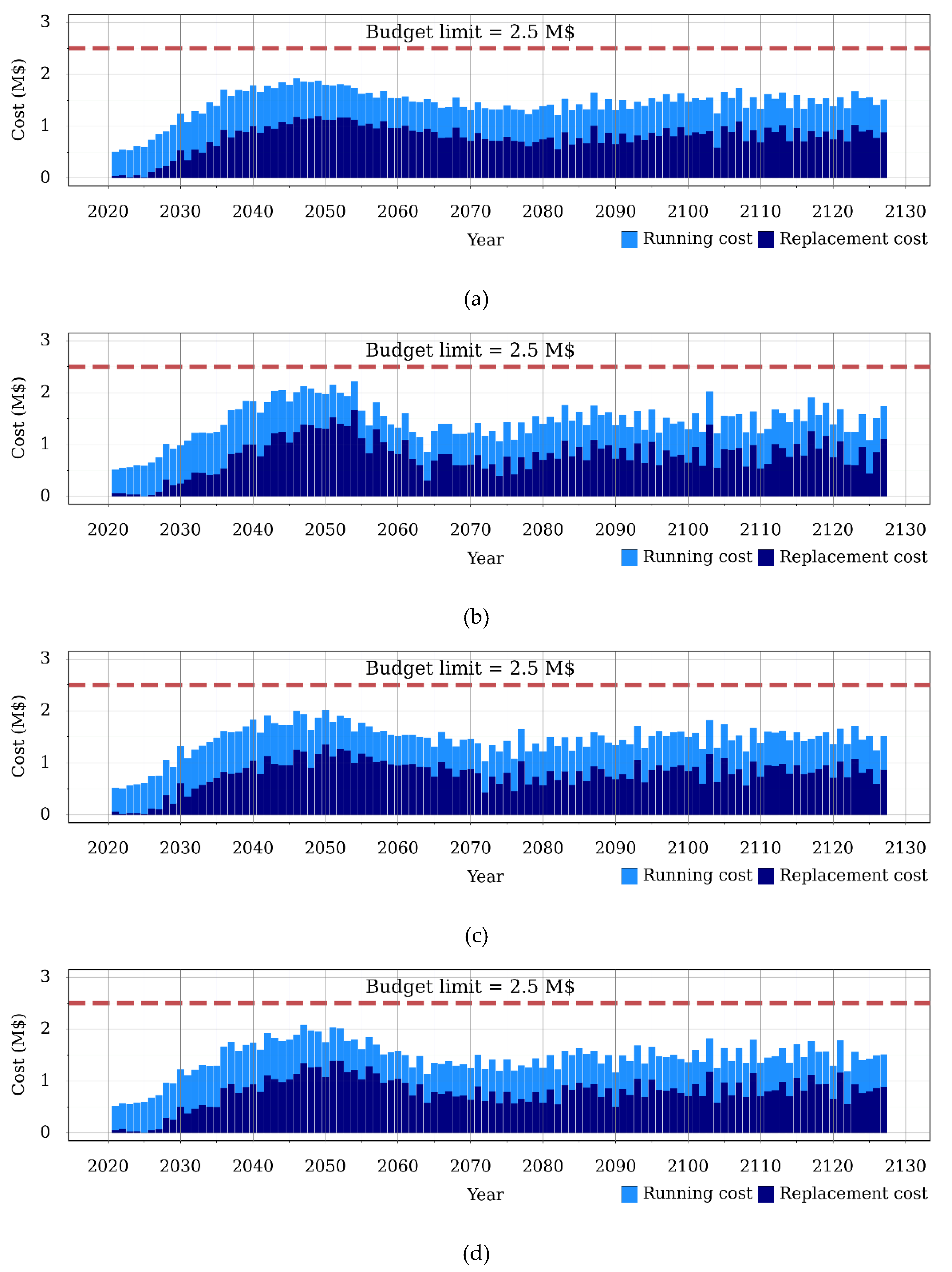
The investment time series obtained by the four representative solutions of the first scenario are shown in Figure 10, and the details are summarized in Table 4. In Figure 10, the red dashed line indicates the annual budget limit. The first scheduling plan (Solution 1, shown in Figure 10a) shows the smoothest time series with the minimum SD of annual investment. The second scheduling plan (Solution 2, shown in Figure 10b) is the closest to LLCCN and therefore has the lowest imposed cost. The third scheduling plan (Solution 3, shown in Figure 10c) yields the youngest network with the lowest pipe average age, which can be considered as a more reliable plan than other solutions. The use of the knee-point (Solution 4) provides a balanced scheduling plan that considers all three objective functions simultaneously, as shown in Figure 10d.
In Table 4, MODE represents the pipe replacement year relative to the with the highest frequency; that is, the year picked most often as the new replacement time for pipes in the network. The maximum represents the maximum annual investment value. The objective of this study was to minimize and disperse this maximum annual investment compared to the LLCCN schedule to provide the smallest fluctuation in annual expenditure. The running and initial costs and their summation after changing the replacement time represent the change in expenditure due to the selection of a different budget and replacement boundary. When the replacement time is postponed by 5 years from the expected in the first scenario, a 5-year running cost is added to the new plan, therefore 5 years are added to its life cycle. On the other hand, when a pipe is replaced 5 years sooner than the expected , 5 years are omitted from its life cycle, which reduces the running cost and pipe age, but increases the replacement cost. The TAI, defined as the total cost divided by the time horizon (i.e., 108 years), provides an estimation of the annual WDN maintenance cost and enables a more realistic budget to be assigned for WDN rehabilitation. Note that the LCC does not depend on the time scale and represents the continuous life cycle of an asset. However, the total cost depends on the time horizon to be investigated; upon changing the time horizon, the total cost changes because the cycle is cut in a particular year. In this case, only the cost up to that specific year is counted. Note that the time horizon of the case study WDN was determined based on the above-mentioned assumption in which all pipes need to be replaced at least once.
As shown in Table 4, for Scenario 1 (in which the replacement boundary was 5 years), the replacement times for the majority of pipes at the edge of the boundary were determined to occur 5 years sooner in order to disperse all the peaks and provide a sufficiently smooth time series.
As shown in Figure 10a, Solution 1 provides the smoothest investment time series with the lowest maximum annual investment of 1.99 M$. This solution shows a 59% decrease in the SD of annual investment compared to the before-smoothing-plan. For Solution 2, the majority of pipe replacement times remained unchanged in order to ensure a small deviation from LLCCN, and the MODE is 0. This solution was obtained to prioritize keeping the replacement time the same as (MODE = 0) while dispersing the peaks as necessary. As shown in Figure 10b, this time series follows the same pattern as the time series before smoothing (Figure 9), but in a smoother manner, and imposed the minimum cost to the network compared to the other solutions, with a maximum annual investment of 2.22 M$, and the LCC marginally increased by 0.08% compared to the before-smoothing-plan. For Solution 3, shown in Figure 10c, the priority was to keep the network younger; as a consequence, the majority of pipes are replaced 5 years sooner than , which results in a more reliable plan than provided by the other three solutions. The average age in this solution decreased by 14.7% compared to the before-smoothing-plan. In Solution 4, which used the knee-point to fairly consider all three objectives, the replacement time can be observed to be dispersed evenly around the provided boundary, as shown in Figure 10d.
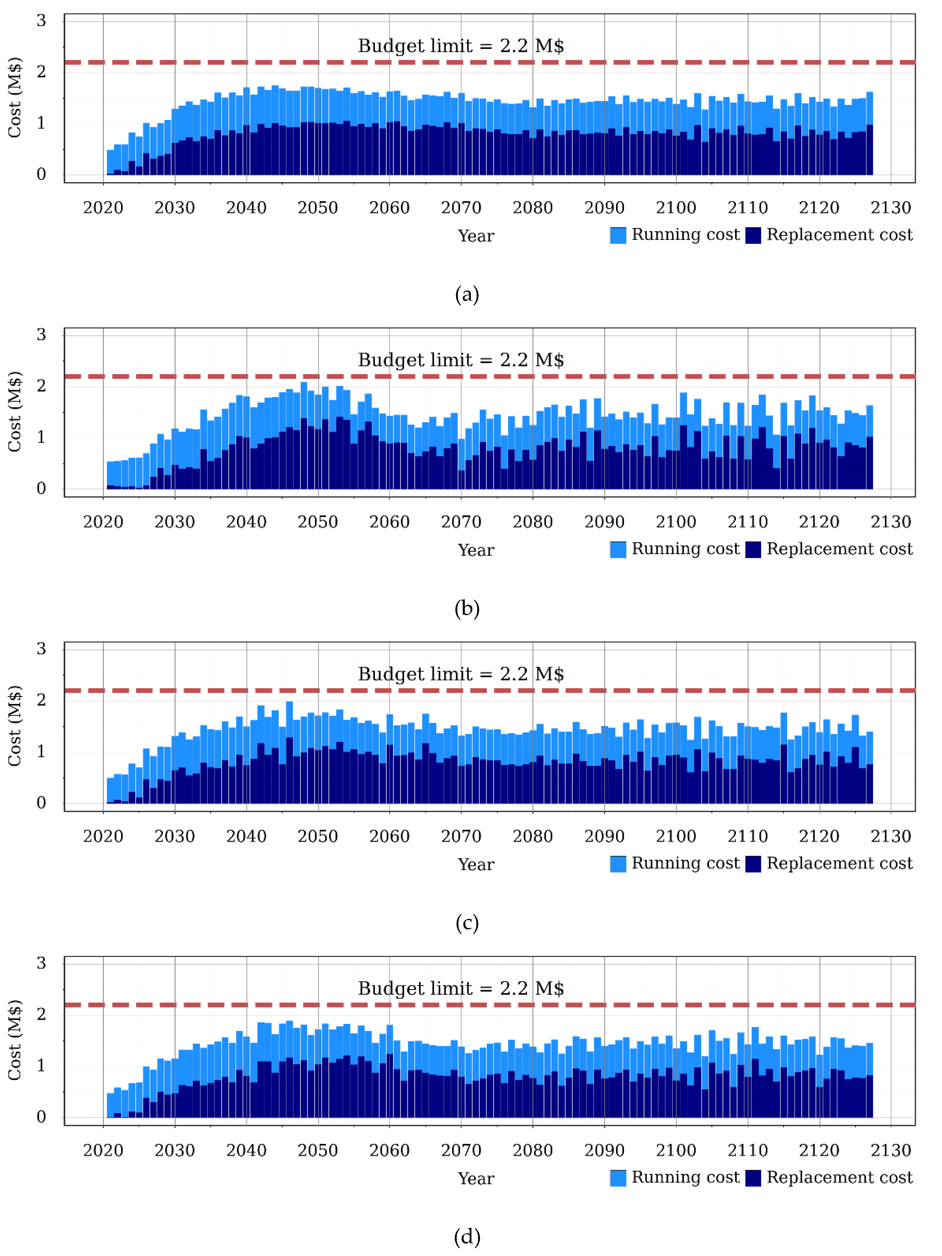
3.3.3. Future Investment Based on Scenario 2
In Scenario 2, the budget limitation decreased to 2.2 M$, and as a consequence, the replacement boundary was increased to 10 years. In this scenario, as shown in Table 5, the MODE for Solution 1 was −10 years, and the replacement times were dispersed to the extent possible to smooth the time series. Consequently, Figure 11a shows a well-smoothed investment time series for Solution 1. The imposed cost for this solution was the highest, while the maximum annual investment was the lowest, leading to a 66.25% smaller SD compared to the before-smoothing-plan. Solution 2 was used to obtain the most economical scheduling plan by keeping the imposed LCC near LLCCN (MODE = 0) and consequently a less smooth curve showing the highest maximum annual investment of 2.18 M$ can be observed in Figure 11b. It is observed that the overall investment of Scenario 2 marginally increases compared to Scenario 1, because the replacement time boundary was relaxed by five additional years. The youngest scheduling plan was provided by Solution 3, which showed a 23.53% reduction compared to the before-smoothing-plan and is shown in Figure 11c.
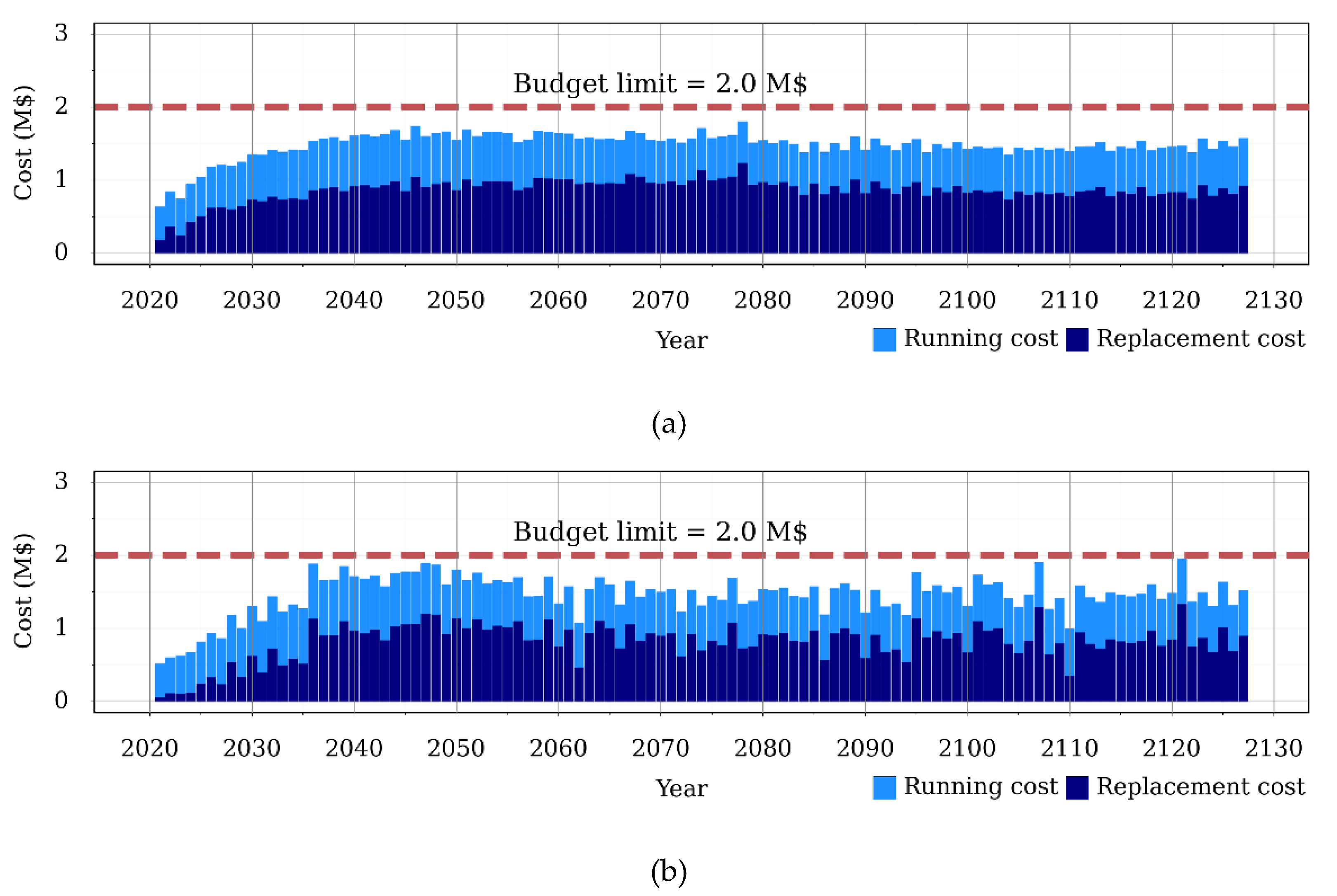
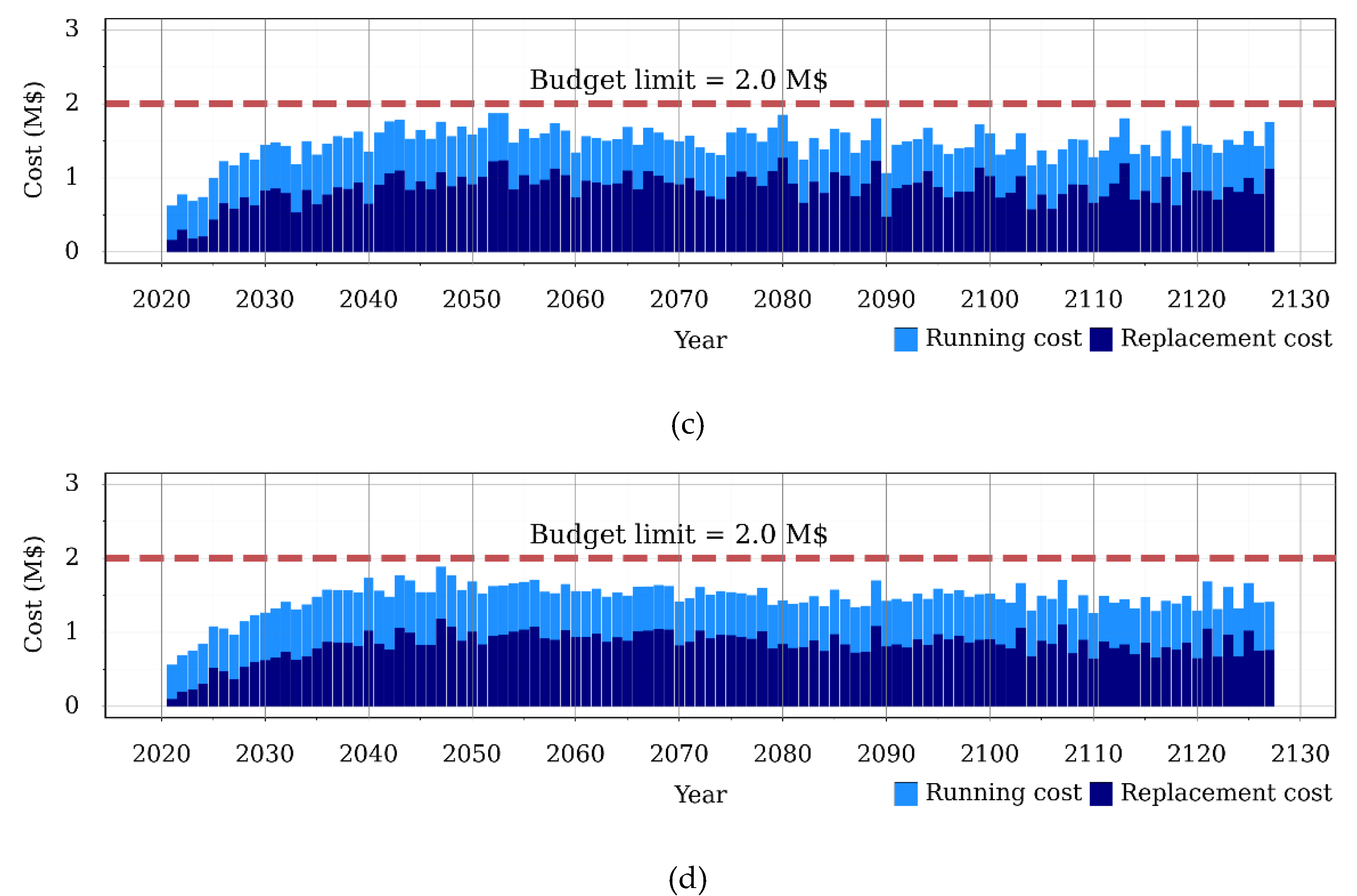
3.3.4. Future Investment Based on Scenario 3
Scenario 3 dispersed the replacement time interval the widest (16 years) with the lowest budget limitation of 2.0 M$. As shown in Figure 12a, the time series for Solution 1 was the smoothest, not only among the four representative solutions in this scenario, but also among all three scenarios, showing a 73.2% reduction in the SD of annual investment compared to the before-smoothing-plan. In Solution 2, the imposed LCC is the minimum (with MODE = 0) while the SD is the maximum as shown in Table 6 and Figure 12b. The most reliable and youngest plan was provided by Solution 3, as shown in Figure 12c. It is interesting to observe that the MODE of Solution 3 is −12 years, which do not reach the LB (i.e., −16 years). This means that the majority of pipes should be replaced later than the LB to refrain from violating the other objectives while minimizing the system age. This indicates that the proposed method acted intelligently in selecting the replacement time and showed reasonable and sensible results. The average age of the network decreased by 26.8% compared to the before-smoothing-plan.
3.3.5. Comparison between Representative Solutions
Table 7 shows a comparison between all three evaluated scenarios in terms of the minimum value of each objective function. First, a notable trade-off can be observed between two constraints, that is, increasing the replacement time boundary could reduce the budget ceiling. Setting the replacement time boundary affects the ability to meet the budget constraints and vice versa. Next, the reason for evaluating these three scenarios was to assess the effect of different budgets and time boundaries in terms of the three objective functions. Scenario 1, with the highest budget limitation and the smallest replacement boundary, provided the lowest-cost scheduling plan in which the imposed LCC was negligible, while the investment time series was fairly smooth due to the small change in replacement time. Whilst, Scenario 3, with the lowest budget limitation and widest replacement range, provided the smoothest and the youngest scheduling plan while imposing the highest LCC on the WDN. The change in the average age of the network from Scenarios 2 to 3 was negligible, while the change in imposed LCC was sufficiently high to make a competitive difference in selecting between these scenarios. On the other hand, there was no significant change in the imposed LCC from Scenarios 1 to 2, while the average age in Scenario 2 implied that its scheduling plan would maintain a reliable WDN by keeping the assets younger. Therefore, Scenario 2 provided a reasonable case that comprehensively considered the three objectives, balancing the smoothness, imposed LCC, and average age of the WDN. This indicates that the proposed method allows decision-makers to consider various scenarios with combinations of annual budget and replace time span and select the most appropriate solution as required.
The optimal scheduling plans obtained in Scenarios 1, 2, and 3 increased the LCC marginally by 0.08%, 0.27%, and 1.06%, respectively, from the LLCC. In terms of smoothness, a well-prorated investment time series was obtained with small fluctuations in annual investment by dispersing the peak annual investment of 3.36 M$ and smoothing to 1.99, 1.80, and 1.79 M$ for Solutions 1 in Scenarios 1, 2, and 3, respectively. In all three scenarios, moving from Solution 1 to Solution 2 led to an increase in the year-to-year fluctuation in investment but reduced the imposed LCC. Solutions 1 and 3 provided the highest initial cost and, consequently, the lowest running cost.
Comparing Figure 10, Figure 11 and Figure 12 with Figure 9, the investment time series clearly becomes smoother, and the fluctuation in annual investment decreases due to the optimal scheduling of pipe replacements. In addition, it can be observed that among the four representative solutions evaluated, Solution 1 provided a well-prorated plan that can make the budget allocations easier than in Solutions 2 and 3. Budget allocation is an essential issue in water infrastructure asset management that increases system reliability by considering all the assets in the budget allocation process. Thus, using the proposed method will help water infrastructure managers by improving their ability to assign a realistic budget that better matches the reality of the system and the financial structure by which it is maintained.
4. Conclusions
The NSGA-II was tuned to develop a multi-objective optimization model used to solve a pipe replacement scheduling problem of WDN. Three scenarios with different replacement time boundaries and budget limitations were defined by targeting the minimum imposed LCC, minimum SD of the annual investment, and minimum average age of the WDN. For individual pipes in a real-life WDN, the results of the simulation proposed the replacement times, and four scheduling plans were evaluated based on four different budgetary viewpoints and decision-maker opinions. We confirmed that the optimization provides a helpful decision-making result to visualize the trade-offs among pipe replacement schedules. The following conclusions were derived based on the proposed scheduling plan.
Using the proposed scheduling framework, a useful number of service years was obtained for all individual pipes, and rehabilitation management was performed more efficiently. For a large WDN with ductile iron pipe diameters of 80–500 mm in an age range of 4–53 years, smoothed investment time series were proposed using three different scenarios. We ranked four different solutions for each scenario based on a real field situation and decision-maker opinions, obtaining twelve alternative scheduling plans that better match reality.
The running cost used in this study plays an essential role in developing the investment time series; therefore, data analytics and techniques for the control and management of a large-scale WDN are needed. By using online monitoring and recording failure data, the pipe failure rate could be continuously updated. Thus, by updating the annual replacement plan over years of monitoring, the accuracy of the failure rate would be improved and the running cost would therefore become more realistic, allowing the scheduling plan to become near-optimal.
The methods employed in this study can be extended in future research to investigate different rehabilitation scenarios (i.e., repair and renovation) and techniques (i.e., sleeves, CIPP) considering more components and other pipe materials.
Author Contributions
F.G. carried out the analysis of the proposed method, model simulations, and drafted the manuscript; G.J. surveyed the previous studies and analyzed the network; D.K. provided the original idea of the study and finalized the manuscript. All authors have read and agreed to the published version of the manuscript.
Funding
This research was supported by the EDISON (Education-research Integration through Simulation on the Net) Program through the National Research Foundation of Korea (NRF) funded by the Ministry of Science, ICT & Future Planning (2017M3C 1A6075016).
Institutional Review Board Statement
Not applicable.
Informed Consent Statement
Not applicable.
Data Availability Statement
The data presented in this study are available on request from the corresponding author. The data are not publicly available due to privacy.
Conflicts of Interest
The authors declare no conflict of interest.
References
- Shahnawaz, K. Design Improvement in Water Distribution Systems: A Life Cycle Thinking Approach. Master’s Thesis, University of British Columbia, Vancouver, BC, Canada, 2019. [Google Scholar]
- Zhou, Y. Deterioration and Optimal Rehabilitation Modelling for Urban Water Distribution Systems; CRC Press: Boca Raton, FL, USA, 2018. [Google Scholar]
- Selvakumar, A.; Clark, R.M.; Sivaganesan, M. Costs for Water Supply Distribution System Rehabilitation. J. Water Resour. Plan. Manag. 2002, 128, 303–306. [Google Scholar] [CrossRef]
- Shin, H.; Joo, C.; Koo, J. Optimal Rehabilitation Model for Water Pipeline Systems with Genetic Algorithm. Procedia Eng. 2016, 154, 384–390. [Google Scholar] [CrossRef] [Green Version]
- Li, F.; Ma, L.; Sun, Y.; Mathew, J. Optimized Group Replacement Scheduling for Water Pipeline Network. J. Water Resour. Plan. Manag. 2016, 142, 04015035. [Google Scholar] [CrossRef]
- Gill, N.; Shah, J. Which Pipe First? Using Evidence-Based Condition Assessment and Desktop Modeling to Optimize Pipe Replacement. In Pipelines 2019: Condition Assessment, Construction, and Rehabilitation; American Society of Civil Engineers: Reston, VA, USA, 2019; pp. 417–423. [Google Scholar] [CrossRef]
- Olsson, R.J.; Kapelan, Z.; Savić, D.A. Probabilistic building block identification for the optimal design and rehabilitation of water distribution systems. J. Hydroinform. 2009, 11, 89–105. [Google Scholar] [CrossRef] [Green Version]
- Tanyimboh, T.T.; Kalungi, P. Optimal long-term design, rehabilitation and upgrading of water distribution networks. Eng. Optim. 2008, 40, 637–654. [Google Scholar] [CrossRef]
- Marzouk, M.; Osama, A. Fuzzy-Based Methodology for Integrated Infrastructure Asset Management. Int. J. Comput. Intell. Syst. 2017, 10, 745. [Google Scholar] [CrossRef] [Green Version]
- Giustolisi, O.; Laucelli, D.; Savic, D.A. Development of rehabilitation plans for water mains replacement considering risk and cost-benefit assessment. Civ. Eng. Environ. Syst. 2006, 23, 175–190. [Google Scholar] [CrossRef]
- Fu, G.; Kapelan, Z.; Kasprzyk, J.R.; Reed, P. Optimal Design of Water Distribution Systems Using Many-Objective Visual Analytics. J. Water Resour. Plan. Manag. 2013, 139, 624–633. [Google Scholar] [CrossRef] [Green Version]
- Zhou, Y. Optimal Rehabilitation Decision Model. In Deterioration and Optimal Rehabilitation Modelling for Urban Water Distribution Systems; CRC Press: Boca Raton, FL, USA, 2018; pp. 101–161. [Google Scholar]
- Shamir, U.; Howard, C.D. An Analytic Approach to Scheduling Pipe Replacement. J. Am. Water Work. Assoc. 1979, 71, 248–258. [Google Scholar] [CrossRef]
- Walski, T.M.; Pelliccia, A. Economic analysis of water main breaks. J. Am. Water Work. Assoc. 1982, 74, 140–147. [Google Scholar] [CrossRef]
- Kleiner, Y.; Adams, B.J.; Rogers, J.S. Long-term planning methodology for water distribution system rehabilitation. Water Resour. Res. 1998, 34, 2039–2051. [Google Scholar] [CrossRef]
- Dandy, G.C.; Engelhardt, M.O. Optimal Scheduling of Water Pipe Replacement Using Genetic Algorithms. J. Water Resour. Plan. Manag. 2001, 127, 214–223. [Google Scholar] [CrossRef]
- Alvisi, S.; Franchini, M. Multiobjective Optimization of Rehabilitation and Leakage Detection Scheduling in Water Distribution Systems. J. Water Resour. Plan. Manag. 2009, 135, 426–439. [Google Scholar] [CrossRef]
- Tee, K.F.; Khan, L.R.; Chen, H.P.; Alani, A.M. Reliability based life cycle cost optimization for underground pipeline networks. Tunn. Undergr. Space Technol. 2014, 43, 32–40. [Google Scholar] [CrossRef]
- Karamouz, M.; Yaseri, K.; Nazif, S. Reliability-Based Assessment of Lifecycle Cost of Urban Water Distribution Infrastructures. J. Infrastruct. Syst. 2017, 23, 04016030. [Google Scholar] [CrossRef]
- Nafi, A.; Kleiner, Y. Scheduling Renewal of Water Pipes While Considering Adjacency of Infrastructure Works and Economies of Scale. J. Water Resour. Plan. Manag. 2010, 136, 519–530. [Google Scholar] [CrossRef] [Green Version]
- Fuchs-Hanusch, D.; Kornberger, B.; Friedl, F.; Scheucher, R. Whole of life cost calculations for water supply pipes. In Asset Management of Water and Wastewater Infrastructure, including Technical and Socioeconomic Aspects; LESAM 2011 Strategic Asset Management of Water and Wastewater Infrastructure, Mühlheim; International Water Association: London, UK, 27–30 September 2011; Volume 8, pp. 19–24. [Google Scholar]
- Estevan, H.; Schaefer, B. Life Cycle Costing State of the Art Report, ICLEI–Local Governments for Sustainability; European Secretariat: Bonn, Germany, 2017; pp. 4–11. [Google Scholar]
- Gransberg, D. Life Cycle Costing for Engineers. Constr. Manag. Econ. 2010, 28, 1113–1114. [Google Scholar] [CrossRef]
- Lee, H.; Shin, H.; Rasheed, U.; Kong, M. Establishment of an Inventory for the Life Cycle Cost (LCC) Analysis of a Water Supply System. Water 2017, 9, 592. [Google Scholar] [CrossRef]
- Jayaram, N.; Srinivasan, K. Performance-based optimal design and rehabilitation of water distribution networks using life cycle costing. Water Resour. Res. 2008, 44, 1–15. [Google Scholar] [CrossRef]
- Roshani, E.; Filion, Y.R. Event-Based Approach to Optimize the Timing of Water Main Rehabilitation with Asset Management Strategies. J. Water Resour. Plan. Manag. 2014, 140, 04014004. [Google Scholar] [CrossRef] [Green Version]
- Frangopol, D.M.; Soliman, M.S. Life-cycle of structural systems: recent achievements and future directions. Struct. Infrastruct. Eng. 2016, 12, 1–20. [Google Scholar] [CrossRef]
- Godfrey, S.; Hailemichael, G. Life cycle cost analysis of water supply infrastructure affected by low rainfall in Ethiopia. J. Water, Sanit. Hyg. Dev. 2017, 7, 601–610. [Google Scholar] [CrossRef]
- Hasegawa, K.; Arai, Y.; Koizumi, A. Life Cycle Cost-based Pipe Replacement Model and Application in Depopulation Scenario. In Proceedings of the WDSA/CCWI Joint Conference, Kingston, ON, Canada, 23–25 July 2018. [Google Scholar]
- Elsayed, E.A. Life Cycle Costs and Reliability Engineering. In Wiley StatsRef: Statistics Reference Online; Wiley: Hoboken, NJ, USA, 2014; pp. 1–10. [Google Scholar]
- U.S. Army Corps of Engineers. Engineering and Design-Evaluation of Existing Water Distribution Systems; Engineer Technical Letter No. 1110-2-278; U.S. Army Corps of Engineers: Washington, DC, USA, 1983. [Google Scholar]
- Jardine, A.K.S.; Tsang, A.H.C. Maintenance, Replacement, and Reliability Theory and Applications, 2nd ed.; CRC Press: Boca Raton, FL, USA, 2013; ISBN 9789896540821. [Google Scholar]
- Deb, K.; Agrawal, S.; Pratap, A.; Meyarivan, T. A Fast Elitist Non-Dominated Sorting Genetic Algorithm for Multi-Objective Optimization: NSGA-II; Lect. Notes Comput. Sci.; including Subser. Lect. Notes Artif. Intell. Lect. Notes Bioinformatics; Springer: Heidelberg/Berlin, Germany, 2000; Volume 1917, pp. 849–858. [Google Scholar] [CrossRef]
- Wang, H.; Chen, X. Optimization of Maintenance Planning for Water Distribution Networks under Random Failures. J. Water Resour. Plan. Manag. 2016, 142, 04015063. [Google Scholar] [CrossRef]
- K-water. Water Facilities Construction Cost Estimation Report; Technical Report; K-water: Daejeon, Korea, 2010. [Google Scholar]
- Blank, J.; Deb, K. Pymoo: Multi-Objective Optimization in Python. IEEE Access 2020, 8, 89497–89509. [Google Scholar] [CrossRef]
Figure 1.
Example of life cycle cost (LCC) curve for obtaining the optimal pipe replacement age.

Figure 2.
Selection of replacement time interval based on LCC curve.

Figure 3.
Annual investment time series without smoothing (the dashed line indicates an annual budget limit).
Figure 3.
Annual investment time series without smoothing (the dashed line indicates an annual budget limit).

Figure 4.
General flowchart of NSGA-II.

Figure 5.
Case study network layout according to (a) different pipe diameters and (b) different pipe ages.
Figure 5.
Case study network layout according to (a) different pipe diameters and (b) different pipe ages.

Figure 6.
Optimal replacement time () for each pipe diameter based on LCC assessment.

Figure 7.
Comparison of nondominated Pareto solutions for three scenarios.

Figure 8.
Two-dimensional projections of nondominated Pareto solutions for three scenarios: (a) comparison between average age and imposed LCCN, (b) comparison between average age and SD of annual investment, and (c) comparison between imposed LCCN and SD of annual investment.
Figure 8.
Two-dimensional projections of nondominated Pareto solutions for three scenarios: (a) comparison between average age and imposed LCCN, (b) comparison between average age and SD of annual investment, and (c) comparison between imposed LCCN and SD of annual investment.


Figure 9.
Future investment time series before smoothing.

Figure 10.
Future investment time series for Scenario 1: (a) Solution 1—min. SD of annual investment, (b) Solution 2—min. imposed LCC, (c) Solution 3—min. system age, and (d) Solution 4—knee-point.
Figure 10.
Future investment time series for Scenario 1: (a) Solution 1—min. SD of annual investment, (b) Solution 2—min. imposed LCC, (c) Solution 3—min. system age, and (d) Solution 4—knee-point.

Figure 11.
Future investment time series for Scenario 2: (a) Solution 1—min. SD of annual investment, (b) Solution 2—min. imposed LCC, (c) Solution 3—min. system age, and (d) Solution 4—knee-point.
Figure 11.
Future investment time series for Scenario 2: (a) Solution 1—min. SD of annual investment, (b) Solution 2—min. imposed LCC, (c) Solution 3—min. system age, and (d) Solution 4—knee-point.

Figure 12.
Future investment time series for Scenario 3: (a) Solution 1—min. SD of annual investment, (b) Solution 2—min. imposed LCC, (c) Solution 3—min. system age, and (d) Solution 4—knee-point.
Figure 12.
Future investment time series for Scenario 3: (a) Solution 1—min. SD of annual investment, (b) Solution 2—min. imposed LCC, (c) Solution 3—min. system age, and (d) Solution 4—knee-point.


Table 1.
Initial cost data of ductile iron pipe [35].
Table 1.
Initial cost data of ductile iron pipe [35].
| Diameter (mm) | Pipe Cost ($/m) | ||
|---|---|---|---|
| Material | Construction | Total | |
| 80 | 15 | 65 | 80 |
| 100 | 28 | 66 | 94 |
| 150 | 41 | 76 | 117 |
| 200 | 59 | 86 | 145 |
| 250 | 81 | 96 | 177 |
| 300 | 103 | 105 | 208 |
| 350 | 125 | 114 | 239 |
| 400 | 149 | 127 | 276 |
| 450 | 156 | 136 | 292 |
| 500 | 182 | 148 | 330 |
Table 2.
LLCC (least life cycle cost) and corresponding replacement age () for different diameters.
| Diameter (mm) | CI ($/km/Year) | CR ($/km/Year) | LLCC ($/km/Year) | |
|---|---|---|---|---|
| 80 | 35 | 2286 | 1725 | 4010 |
| 100 | 37 | 2541 | 1878 | 4418 |
| 150 | 42 | 2786 | 2080 | 4865 |
| 200 | 49 | 2959 | 2223 | 5182 |
| 250 | 57 | 3105 | 2275 | 5380 |
| 300 | 67 | 3104 | 2304 | 5408 |
| 350 | 78 | 3064 | 2264 | 5327 |
| 400 | 91 | 3033 | 2203 | 5236 |
| 450 | 104 | 2808 | 2065 | 4873 |
| 500 | 122 | 2705 | 1991 | 4696 |
Table 3.
Details of the investment before smoothing.
| Standard Deviation (M$) | LLCCN (M$/year) | Average Age (Year) | Running Cost (M$) | Initial Cost (M$) | Total Cost (M$) | TAI (M$/Year) | |
|---|---|---|---|---|---|---|---|
| 0.72 | 1.504 | 27.2 | 3.36 | 70.28 | 90.65 | 160.93 | 1.490 |
Table 4.
Details of four selected points for Scenario 1 (replacement time boundary = 5 years, annual budget limit = 2.5 M$).
Table 4.
Details of four selected points for Scenario 1 (replacement time boundary = 5 years, annual budget limit = 2.5 M$).
| Solution Number | Standard Deviation (M$) | Imposed LCC (k$/Year) | Average Age (Year) | MODE (Year) | Running Cost (M$) | Initial Cost (M$) | Total Cost (M$) | TAI (M$/Year) | |
|---|---|---|---|---|---|---|---|---|---|
| 1 | 0.298 | 3.8 | 23.5 | −5 | 1.99 | 69.70 | 90.66 | 160.36 | 1.485 |
| 2 | 0.381 | 1.3 | 24.2 | 0 | 2.22 | 70.53 | 89.48 | 160.00 | 1.481 |
| 3 | 0.315 | 3.5 | 23.2 | −5 | 2.08 | 69.72 | 90.61 | 160.33 | 1.485 |
| 4 | 0.332 | 2.2 | 23.6 | 0 | 2.15 | 70.15 | 90.22 | 160.37 | 1.485 |
Table 5.
Details of four selected points for Scenario 2 (replacement time boundary = 10 years, annual budget limit = 2.2 M$).
Table 5.
Details of four selected points for Scenario 2 (replacement time boundary = 10 years, annual budget limit = 2.2 M$).
| Solution Number | Standard Deviation (M$) | Imposed LCC (k$/Year) | Average Age (Year) | MODE (Year) | Running Cost (M$) | Initial Cost (M$) | Total Cost (M$) | TAI (M$/Year) | |
|---|---|---|---|---|---|---|---|---|---|
| 1 | 0.243 | 15 | 22.4 | −10 | 1.80 | 68.27 | 92.79 | 161.06 | 1.491 |
| 2 | 0.342 | 4 | 22.2 | 0 | 2.18 | 69.83 | 90.56 | 160.39 | 1.485 |
| 3 | 0.268 | 10 | 20.8 | −10 | 2.08 | 68.03 | 92.82 | 160.86 | 1.489 |
| 4 | 0.278 | 8 | 21.2 | −3 | 1.97 | 68.48 | 92.07 | 160.56 | 1.487 |
Table 6.
Details of four selected points for Scenario 3 (replacement time boundary =16 years, annual budget limit = 2.0 M$).
Table 6.
Details of four selected points for Scenario 3 (replacement time boundary =16 years, annual budget limit = 2.0 M$).
| Solution Number | Standard Deviation (M$) | Imposed LCC (k$/Year) | Average Age (Year) | MODE (Year) | Running Cost (M$) | Initial Cost (M$) | Total Cost (M$) | TAI (M$/year) | |
|---|---|---|---|---|---|---|---|---|---|
| 1 | 0.193 | 51 | 22.2 | −10 | 1.79 | 66.47 | 98.61 | 165.08 | 1.523 |
| 2 | 0.290 | 16 | 21.1 | 0 | 1.97 | 68.56 | 93.00 | 161.57 | 1.496 |
| 3 | 0.240 | 36 | 19.9 | −12 | 1.90 | 65.82 | 97.85 | 163.67 | 1.515 |
| 4 | 0.226 | 28 | 20.7 | −5 | 1.91 | 67.43 | 94.87 | 162.31 | 1.503 |
Table 7.
Comparison of three evaluated scenarios.
| Scenarios | Budget Constraint (M$) | Replacement Time Span [LB,UB] (Year) | Minimum Standard Deviation (M$) | Minimum Imposed LCC (k$/Year) | Minimum Average Age (Year) |
|---|---|---|---|---|---|
| 1 | 2.5 | −5, 5 | 0.298 | 1.3 | 23.2 |
| 2 | 2.2 | −10, 10 | 0.243 | 4.0 | 20.8 |
| 3 | 2.0 | −16, 16 | 0.193 | 16.0 | 19.9 |
Publisher’s Note: MDPI stays neutral with regard to jurisdictional claims in published maps and institutional affiliations. |
© 2021 by the authors. Licensee MDPI, Basel, Switzerland. This article is an open access article distributed under the terms and conditions of the Creative Commons Attribution (CC BY) license (http://creativecommons.org/licenses/by/4.0/).
Share and Cite
MDPI and ACS Style
Ghobadi, F.; Jeong, G.; Kang, D. Water Pipe Replacement Scheduling Based on Life Cycle Cost Assessment and Optimization Algorithm. Water 2021, 13, 605. https://doi.org/10.3390/w13050605
AMA Style
Ghobadi F, Jeong G, Kang D. Water Pipe Replacement Scheduling Based on Life Cycle Cost Assessment and Optimization Algorithm. Water. 2021; 13(5):605. https://doi.org/10.3390/w13050605
Chicago/Turabian StyleGhobadi, Fatemeh, Gimoon Jeong, and Doosun Kang. 2021. "Water Pipe Replacement Scheduling Based on Life Cycle Cost Assessment and Optimization Algorithm" Water 13, no. 5: 605. https://doi.org/10.3390/w13050605
Note that from the first issue of 2016, this journal uses article numbers instead of page numbers. See further details here.