Principal Determinants of Aquatic Macrophyte Communities in Least-Impacted Small Shallow Lakes in France


1
Aquabio, 10 Rue Hector Guimard, 63800 Cournon-d’Auvergne, France
2
University of Rennes, CNRS, ECOBIO-UMR 6553, 35042 Rennes, France
*
Author to whom correspondence should be addressed.
Water 2021, 13(5), 609; https://doi.org/10.3390/w13050609
Submission received: 22 December 2020
/
Revised: 17 February 2021
/
Accepted: 20 February 2021
/
Published: 26 February 2021
(This article belongs to the Section Water Quality and Contamination)
Abstract
:Small shallow lakes (SSL) support exceptionally high and original biodiversity, providing numerous ecosystem services. Their small size makes them especially sensitive to anthropic activities, which cause a shift to dysfunctional turbid states and induce loss of services and biodiversity. In this study we investigated the relationships between environmental factors and macrophyte communities. Macrophytes play a crucial role in maintaining functional clear states. Better understanding the factors determining the composition and richness of aquatic plant communities in least-impacted conditions may be useful to protect these shallow lakes. We inventoried macrophyte communities and collected chemical, climatic, and morphological data from 89 least-impacted SSL widely distributed in France. SSL were sampled across four climatic ecoregions, various geologies, and elevations. Hierarchical cluster analysis showed a clear separation of four macrophyte assemblages strongly associated with mineralization. Determinant factors identified by distance-based redundancy analysis (db-RDA) analysis were, in order of importance, geology, distance from source (DIS, a proxy for connectivity with river hydrosystems), surface area, climate, and hydroperiod (water permanency). Surprisingly, at a country-wide scale, climate and hydroperiod filter macrophyte composition weakly. Geology and DIS are the major determinants of community composition, whereas surface area determines floristic richness. DIS was identified as a determinant in freshwater lentic ecosystems for the first time.
Keywords:
depressional wetlands; ponds; alkalinity; geology; distance from source; connectivity; climate; altitude; hydroperiod1. Introduction
Human activities such as fish stocking, impoundment, or mineral extraction have induced the creation of numerous small shallow lakes (hereafter SSL) [1,2]. The term SSL includes both man-made and natural waterbodies. These freshwater ecosystems are the most abundant on Earth [3]. The mean depth of SSL in temperate regions is less than 3 m, but can reach 7 m [4], and their surface area ranges from 1 m2 to 100 ha [5]. In this study we focused on waterbodies with a surface are less than 50 ha. Waterbodies with a surface area greater than 50 ha are usually monitored in France according to system A from the EU Water Framework Directive (Annex II, 2000/60/EC). SSL can be largely colonized by macrophytes, and do not have persistent stratification for long periods in summer [6]. Obviously, intense sediment–water interaction and the potentially large impact of aquatic vegetation make the functioning of SSL different from that of their deeper counterparts [7].
SSL provide many economically valuable services and long-term benefits to society, such as drinking-water supply, irrigation, and aquaculture, and are often used for different types of recreation, such as angling, boating and swimming, or are built for amenity value [8]. They provide habitats for rich and distinct aquatic fauna and flora [9], and also contribute to the preservation of terrestrial biodiversity, such as birds and bats, by providing habitats and food [10,11]. SSL play a role in regional carbon processing, with burial in sediments and the emission of natural greenhouse gases [12], and are useful for carbon sequestration [13]. They retain part of watershed nutrients and contaminants [14,15], and influence river hydrology and hydromorphology [16]. Despite their economic importance and conservation value, SSL are largely neglected by the scientific community [17,18]. In particular, SSL remain little studied in many European countries, including France, although pond loss has reached 90% in many regions [19], due to agricultural intensification, urbanization and, probably, global warming [20,21]. Human pressures on freshwater ecosystems are increasing, through eutrophication and climate change [22], or by the introduction of exotic or native species [23]. Indeed, climatic disruption induces changes in stratification and mixing regime that could increase the frequency of harmful algal blooms, favoring cyanobacteria and altering nutrient and light availability [24]. Furthermore, extensive nutrient loading increases phytoplankton and periphyton growth, increasing turbidity and limiting access to light for macrophytes [25]. When a critical level of turbidity is exceeded, submerged macrophytes disappear, producing shifts from clear to turbid states [26].
The decline of macrophyte beds in these freshwater ecosystems induces a reduction in biodiversity, and has a negative impact on their function since macrophytes play a key role in SSL. When they are least impacted, many SSL are characterized by clear waters with abundant submerged vegetation. Macrophytes have a positive feedback on transparency, maintaining clear-water conditions through: (1) competition with microalgae and excretion of allelochemicals; (2) providing habitats and refuges from fish predation for zooplankton and invertebrates; and (3) providing habitat for piscivorous fish, limiting zooplanktivorous fishes [27]. Macrophytes also provide habitat for numerous other living organisms, such as periphyton [28,29], water birds [30], and amphibians [31]. As primary producers, they often dominate the production of organic matter, absorbing nutrients, ions, and aerial carbon dioxide [32]. Finally, they also strongly attenuate light and wind-driven turbulence, and separate warm surface water and colder bottom waters [33].
In Europe, most studies on the structure and composition of aquatic plant communities have been conducted in Central, Northern, or Mediterranean countries, within an area defined by homogeneous climatic conditions [34]. The aim of this study was to identify the environmental drivers of aquatic macrophyte assemblages in French least-impacted SSL. France is characterized by four of the five European climatic ecoregions and by a high altitudinal gradient. The hydrogeochemistry of SSL in France also varies quite substantially, from mountainous hard rocks to regions dominated by low-lying alluvial deposits. SSL can be found on non-calcareous and calcareous sandy deposits, in bogs, and on calcareous bedrocks. The baseline hydrogeochemical conditions play a fundamental role in regulating the diversity of macrophyte communities [35].
The target waterbodies of this study occupy a wide range of environmental conditions (altitude, climate, geology), although the latitudinal range is relatively small. Our first hypothesis was that the main driver of aquatic plant communities and richness is the biogeochemistry of these lakes, and in particular the mineralization (water mineral content), because nutrient concentrations are generally low in least-impacted conditions. In particular, we expected a lower richness in non-calcareous lakes, because such lakes may support only carbon-limited species. Our second hypothesis was that the distribution is also explained by climatic gradient, because temperature is a determinant factor for macrophyte metabolism [36].
2. Materials and Methods
2.1. Site Selection
We selected 89 SSL ranging from 3 to 3340 m above sea level (asl), and differing in their geology (calcareous to siliceous), substrate type (sand, clay, rock), water supply (rainfall, groundwater, river flow), and surface area (from 1 m2 to 41.4 ha). These SSL included both permanent, semi-permanent (dry only exceptionally, in drought years), and temporary waters [37]. They were selected from four different biogeographical regions: Alpine, Mediterranean, Continental, and Atlantic (Figure 1). They were of natural origin (glacial, alluvial) or the result of human activity. SSL characterized by shading equal or higher to 75% were not included in the analysis, because of their very low floristic richness [38].
2.2. Environmental Data
Environmental data, except for GIS analyses, were collected the same or the year following the macrophyte survey. For estimation of hydroperiod, each site was prospected at least three times at different seasons during a minimum of two years. GIS analyses were conducted mainly in 2020.
The size, altitude, average depth (estimated), maximum depth, shoreline index [39], and % shading were noted for each sampling site; whereas other factors were coded into four or five classes: slope of banks (class 1: <5%; 2: 5%–25%; 3: 25%–50%; 4: 50%–75%; 5: >75%), and hydroperiod (0: Permanent waters; 1: exceptional pluri-annual droughts; 2: short annual droughts; 3: long annual droughts). Distance from source (DIS), was measured using French National Geography Institute topographic maps; this is a proxy for the degree of connectivity between the SSL and a river hydrosystem [40]. If DIS = 0, the SSL was outside a river floodplain. If DIS > 0, the SSL is crossed by a river or located in its floodplain. Where the SSL was itself a source, DIS = length of the longest distance from the banks to the SSL outlet. Where the SSL was a river impoundment, DIS = length from the source of the river to the SLL outlet. Where the SSL was on a river floodplain, DIS = length from the source to the perpendicular formed by the line between the river and the SSL. So, higher values of DIS denote connections with a larger river. Climatic factors, defined by mean annual air temperature, mean annual air temperature amplitude, and mean annual precipitations, were extracted from the French National Institute for Agronomic and Environmental Research INRAE reanalysis [41] of the SAFRAN/France database [42] for the years 2010–2016.
We collected water and sediment samples once only, in the winter following the macrophyte surveys when biological activity is lower and the concentration of inorganic nutrients is potentially the highest [43]. The water and sediments were sampled at the deepest point of the waterbody, with the exception of the impoundments. In this last case, three sediment samples were taken along an upstream-downstream gradient and were mixed to form a single aggregate sample. The top centimeters of sediment were sampled with a sediment corer or with an Ekman grab, depending on the water depth. pH, conductivity, and water color were measured directly in the water column with probes (Multi-parameter WTW 3430, WTW 3630, Hydrolab, YSI, and Exo3 for the usual parameters, and Lovibond MD100 for water color). Additional chemical parameters (Kjeldhal N, ammonium, nitrite, nitrates, total phosphorus, soluble reactive phosphorus, calcium, alkalinity) were analyzed from the water, whereas Kjeldhal N, total phosphorus, soluble reactive phosphorus, organic carbon, and loss on ignition were analyzed from the sediment samples according to French norms by an accredited laboratory.
2.3. Macrophyte Community
Macrophytes were studied during the period of vegetation growth from 2013 to 2018. We sampled all sites once. All macrophytes were surveyed according to a newly-adapted method from the French standard method XPT90-328 [44] and the PSYM protocol [45]. Terrestrial plants and wetland plants growing outside the outer edge of the waterbodies were not recorded. The vegetation abundance was assessed using the XPT90-328 classes (class 1: few individuals; 2: isolated small patches; 3: numerous small patches; 4: large discontinuous patches; 5: large continuous patches). Macrophytes at the outer edge and the shallow part of the site were surveyed while walking or wading in a zig-zag pattern. Deeper water zones were point-sampled from a boat following a zig-zag pattern with a grapnel or a rake.
Samples such as species of Characeae, Ranunculus subg. Batrachium, and mosses were kept in alcohol or dried for identification in the laboratory. We identified all macrophytes (spermatophytes, bryophytes, and Characeae) at species level when it was possible.
The study of the macrophyte community was realized by calculation of four biodiversity indices (taxonomic richness, Shannon–Wiener (1), Pielou’s (2), and Simpson (3) diversity indices) [46]. The Shannon and Simpson diversity indices are the most widely used indices based on species richness, and provide a synthetic image of richness and species distribution. The Simpson and Pielou’s indices are independent of species richness, and depend solely on species distribution [47].
where pi is the proportion of species (i), and S is the number of species.
2.4. Data Analysis
For multivariate analysis, taxa found at one station only were discarded. Singleton macrophyte species were removed to prevent random and uninterpretable fluctuations, and only taxa identified at species level were retained in the analysis [48].
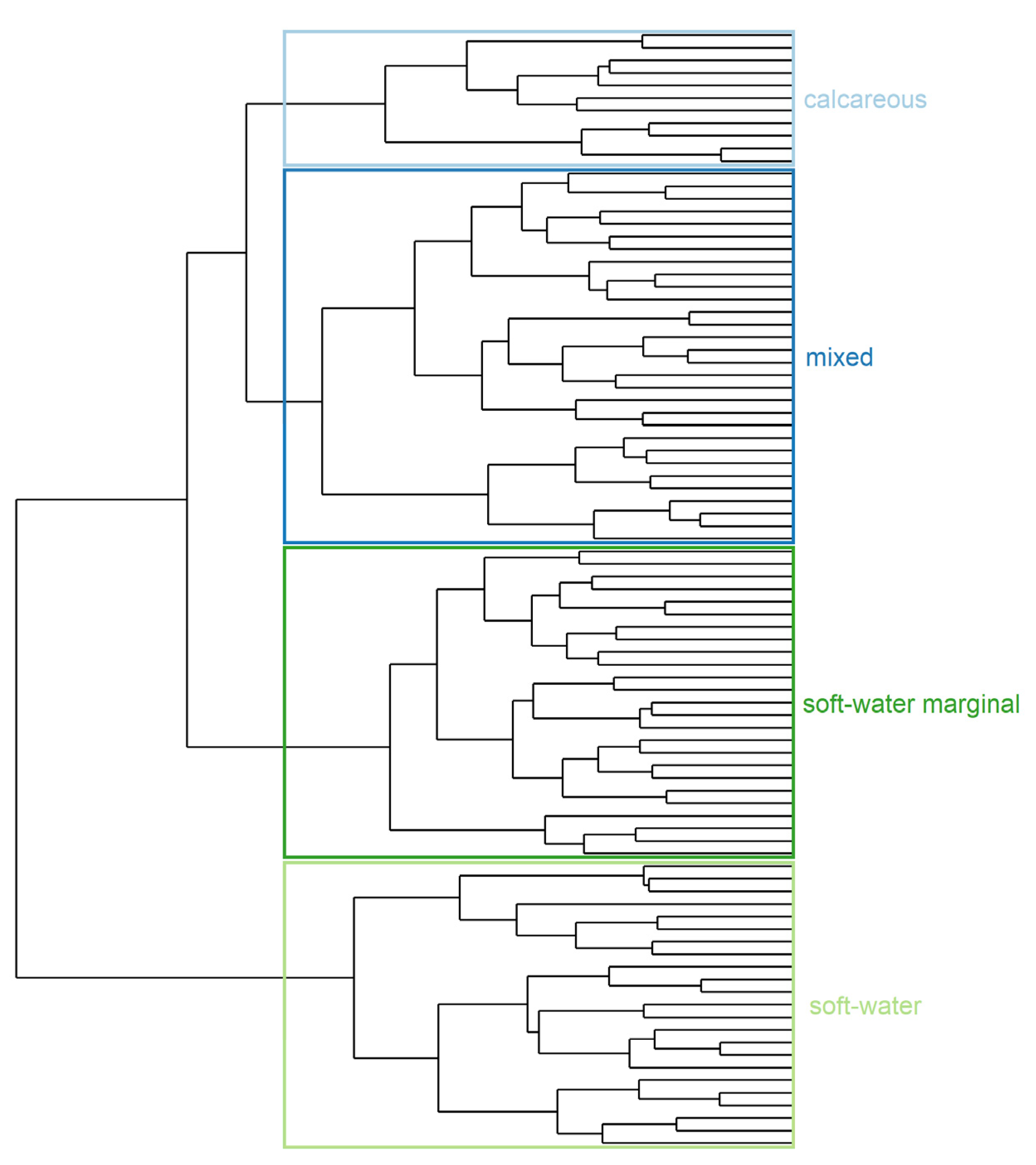
Square-rooted Bray–Curtis dissimilarity was calculated for the abundance-based taxonomic matrix. The dissimilarity matrix was then subjected to a hierarchical cluster analysis using Ward’s minimum variance method, which seeks to define well-delimited groups by minimizing the within-group sum of squares [49].
Community groups were then determined by comparing the distance matrix obtained with dendrogram and binary matrices representing partitions [50]. A category label (Soft-Water, Soft-Water Marginal, Mixed, and Calcareous) was attributed to each community group in accordance with the boundaries of the physico-chemical conditions. Strictly-defined, soft-water lakes are those with Ca <3 mg/L, and with very low alkalinity, whereas soft-water-marginal lakes are characterized by Ca 10–15 mg/L, and higher pH [35]. Calcareous lakes are those with Ca >20 mg/L and alkalinity >1 meq/L [51].
Finally, indicator species for each group were identified using the IndVal index from the indicspecies package [52,53].
IndVal index (4) is a measure of association between a taxon (i) and a group (j) of stations, and is calculated as the product of specificity, A (5) (mean abundance of species i across sites of group j compared to the mean abundance of the species over all groups), and fidelity, B (6) (proportion of sites of a group j with species i). IndVal is maximal (=100%) when a given taxon is observed at all stations of one community group only, and in none of the other groups.
Relationships between environmental factors and groups were explored using pairwise comparisons with Dunn’s tests and boxplots for groups with significant shifts.
Major environmental determinants for macrophyte abundance-based taxonomic composition and groups were identified with distance-based redundancy analysis (db-RDA) [54] combined with parametric forward selection [55], and tested by an ANOVA-like permutation test [56].
Correlations between community characteristics and quantitative environmental variables were assessed using Spearman rank correlations to investigate the intensity of all possible relations following a positive or negative monotonic trend [57]. We used R software [58] for statistical analysis and data plotting. Most of the analysis was processed with the R Vegan package, except Dunn’s test, where the FSA R package was used, and forward selection, which was conducted with the adespatial R package.
3. Results
A total of 183 plant taxa, reduced to 145 after singleton removal, were identified across all 89 stations.
3.1. Community Groups and Environmental Patterns
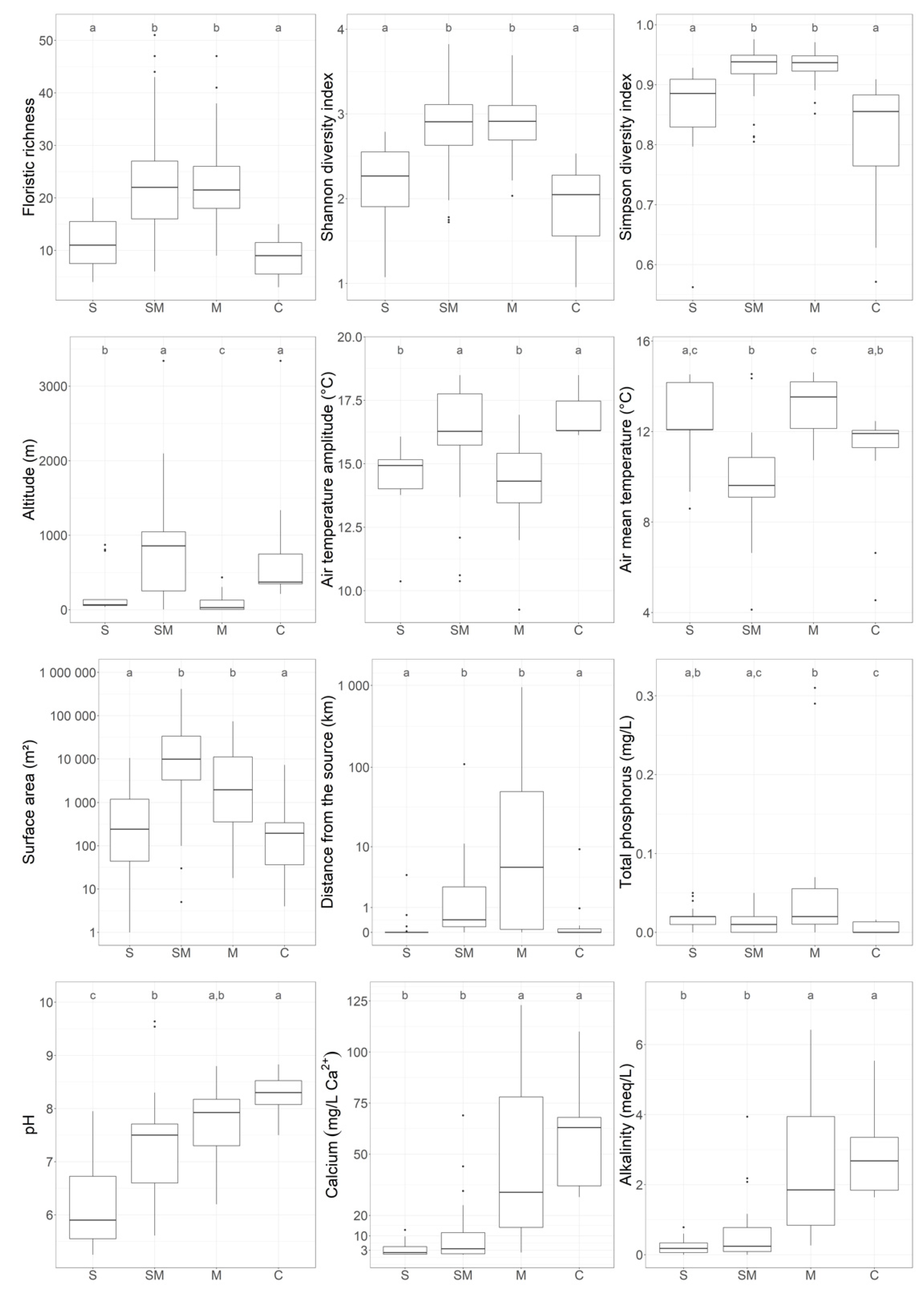
Ward clustering analysis resulted in four defined plant community groups (Figure 2, Table 1) based on the major variables identified by Dunn’s test (alkalinity, calcium, pH, Figure 3, Table S1). The complete record of indicator species for each group, with fidelity, specificity, and indicator values, are provided in Table S2.
The first group of stations corresponded to acid (pH = 5.9 ± 0.8) soft-water lakes (median (calcium) = 1.83 ± 3.25 mg/L, median alkalinity = 0.18 ± 0.21 meq/L). This group pooled together 23 SSL, mostly located at low altitude (<138 m asl), with the exception of three outliers (around 800 m asl). DIS values (median DIS = 0.0 ± 0.8 km) indicated that most of these lakes were not connected to a stream. The indicator species were helophytes, such as Eleocharis multicaulis, hydrophytes, such as Potamogeton polygonifolius, or bryophytes, such as Sphagnum auriculatum (Table 1). The median macrophyte richness was low (n = 11 ± 5).
The second group of stations corresponded to neutral (median pH = 7.5 ± 0.96) soft-water marginal lakes. It comprised 25 SSL. The mineralization level was higher than in the soft-water lake group (median (calcium) = 3.70 ± 16.28 mg/L, median alkalinity 0.24 ± 0.91 meq/L). Most of the rare calcareous fens sampled were strongly associated with this group, and explained the outliers found for calcium, alkalinity, pH, and altitude. SSL from Group 2 were frequently larger than those of the first group. The DIS values (median DIS = 0.4 ± 21.6 km) were higher in this group than those of Group 1, because most of these SSL were upland lakes located close to the source of a stream. This group was defined by numerous helophyte species, such as Carex rostrata or Equisetum fluviatilis, by bryophyte species of the Sphagnum Section cuspidata (mostly S. fallax) and by hydrophyte Ranunculus peltatus. It was characterized by a higher median richness (n = 22 ± 12) than that of the first group.
The third group of stations was the mixed group, with slightly alkaline conditions (median pH = 7.9 ± 0.6). It was characterized by higher mineralization (median (calcium) = 31.35 ± 39.82 mg/L; and alkalinity = 1.85 ± 1.89 meq/L). It grouped together 30 intermediate-hardwater lakes, located in ancient polders, estuaries, or rare geological formations, such as limestone lens on siliceous bedrock. The DIS of these sites showed wide variation (from 0 to 950 km, with median = 5.2 km). The main indicator species were the hydrophyte Potamogeton lucens, the helophyte Phragmites australis, and the bryophyte Leptodictyum riparium. The median richness was similar to that of Group 2 (n = 22 ± 9).
The fourth group of stations, called the calcareous group, comprised 11 alkaline SSL (pH = 8.3 ± 0.36). The group was characterized by its high mineralization level (median (calcium) = 63.00 ± 24.52 mg/L; alkalinity = 2.68 ± 1.17 meq/L), DIS was generally low (DIS = 0.0 ± 2.8km, but with two outliers). Altitude ranged from 213 to 3340 m asl, with a median of 371 m asl. The outlier at 3340 m asl corresponded to a rare calcareous fen with low floristic richness. Group 4 was mostly characterized by submerged macrophyte species, such as Chara contraria, Ranunculus trichophyllus, mosses, such as Drepanocladus aduncus, and by helophyte species such as Juncus articulatus. Species richness was low (median n = 9 ± 4).
3.2. Environmental Drivers of Macrophyte Communities
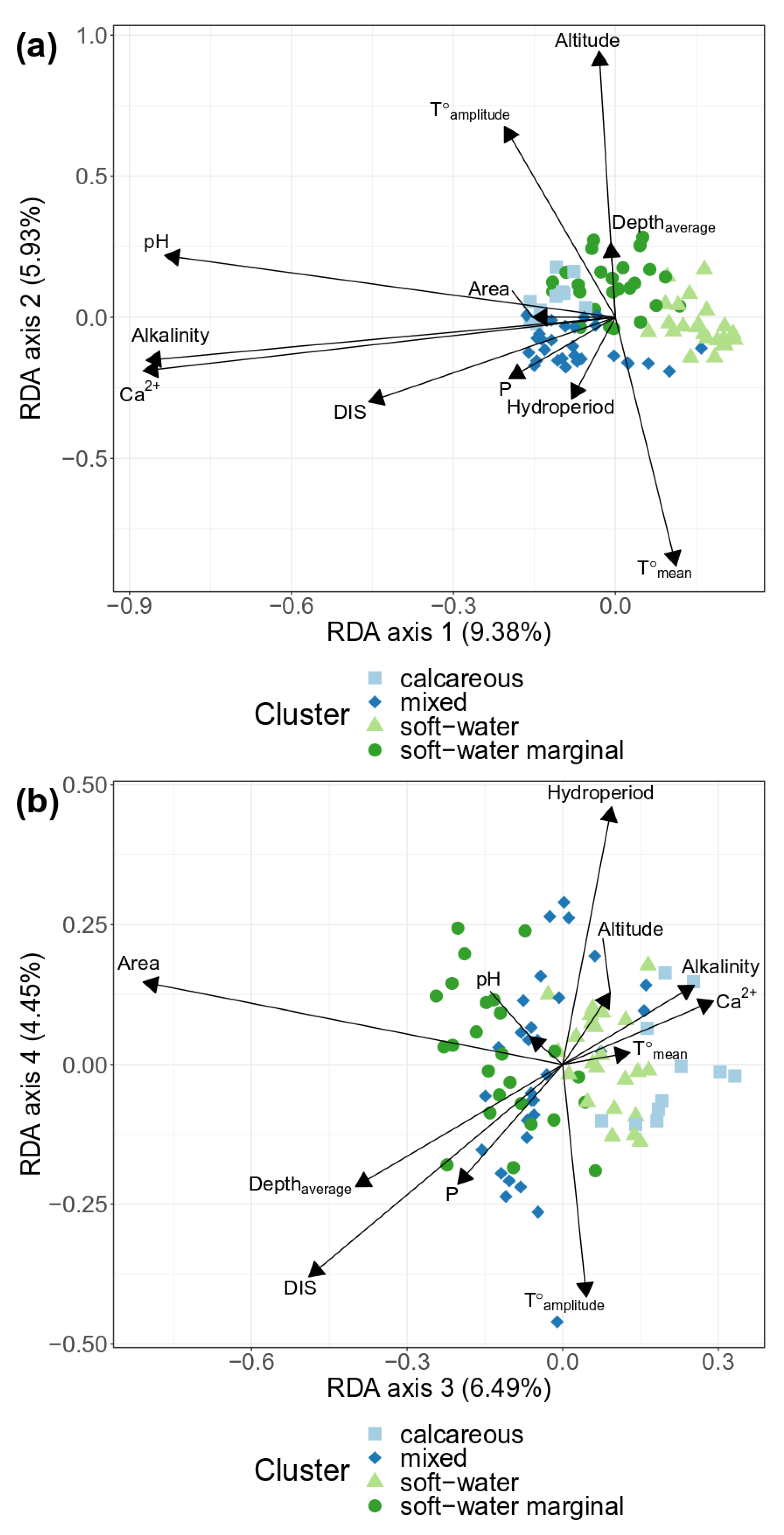
The db-RDA analysis indicated four determinant axes according to the results of the ANOVA-like permutation test (P < 0.001). Two db-RDA biplots, respectively, on the 1–2 axes, and 3–4 axes, are illustrated in Figure 4. In these two biplots, macrophyte communities were significantly influenced by a set of environmental variables that explained a total variation of 26.48%, with the first two axes explaining 15.02%, and the two later axes contributing 11.46% of the db-RDA analysis. Ten variables were retained in the forward selection of the db-RDA model (Table 2).
Variance explained by db-RDA axes are in order of importance, axis 1 (9.38%), axis 3 (6.49%), axis 2 (5.93%), and axis 4 (4.45%).
According to correlations test with db-RDA axes (Table 2), alkalinity (r = −0.79), calcium concentration (r = −0.80), pH (r = −0.76), and DIS (r = −0.41) were negatively correlated with the first db-RDA axis. Surface area (r = −0.67) and DIS (r = −0.40) were negatively correlated with the third db-RDA axis. Altitude (r = 0.87) and air temperature amplitude (r = 0.62) were positively correlated with the second db-RDA axis, whereas mean annual air temperature (r = −0.81) was negatively correlated with this second axis. Hydroperiod (r = 0.37) and air temperature amplitude (r = −0.34) were the environmental factors best correlated with the fourth db-RDA axis (respectively r = 0.37 and r = −0.34).
Total phosphorus was weakly correlated with the fourth db-RDA axis, but showed a strong correlation with DIS (r = 0.70). Finally, mean depth was weakly correlated with the third db-RDA axis (r= 0.33), and a moderate correlation with surface area (r = 0.46) was established.
According to these observations, the ANOVA-like permutation test, and the correlations test with db-RDA axes (Table 2), the best explanatory variables may be classified, in order of importance: (1) Calcium concentration (F = 2.51, P = 0.002) and intercorrelated variables pH and alkalinity; (2) surface area (F = 3.21, P = 0.001); (3) DIS (F = 2.73, P = 0.001) and total phosphorus (F = 2.20, P = 0.004); (4) altitude (F = 2.28, P = 0.006), mean annual air temperature (F = 2.15, P = 0.004), and air temperature amplitude (F = 1.64, P = 0.045); and (5) hydroperiod (F = 1.54, P = 0.049). The influence of mean depth was not significant (P = 0.1).
3.3. Community Characteristics: Biological and Environmental Links
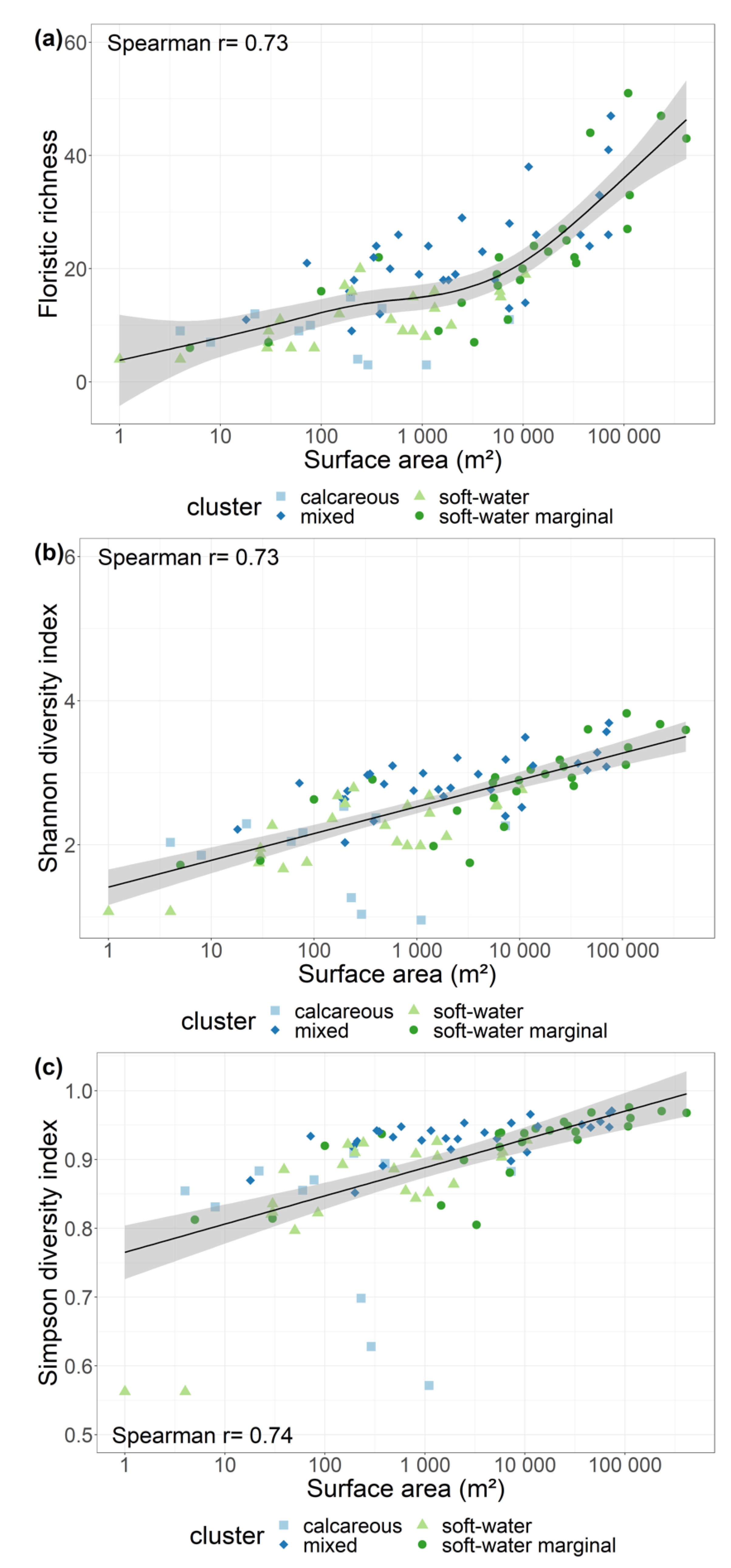
Pielou’s index was not strongly correlated with any environmental variables (Table S3). Among the relationships tested with environmental variables (Table S3, Figure 5), Floristic Richness and Shannon H’ index were strongly positively correlated with surface area (r = 0.73) and perimeter (r = 0.74). Simpson D1 index was strongly negatively correlated with surface area (r = −0.74) and perimeter (r = −0.74).
4. Discussion
4.1. Drivers of Aquatic Plant Community Composition
Our results suggest that mineralization (i.e., alkalinity, calcium concentration) may have a stronger influence than climate on plant distribution and on their abundance at a French scale. The influence of alkalinity on macrophyte species originates from their varying ability to use bicarbonate or carbon dioxide as a source of carbon in photosynthesis [59]. For the first time DIS was found to be among the best explanatory variables for aquatic community composition. DIS is a proxy for connectivity between SSL and river hydrosystems. Being close to a source (DIS close to 0) indicates that SSL are more isolated and have a water chemistry mostly influenced by geology. Increasing values of DIS indicates increased inputs from the catchment area, and a higher chance of an SSL receiving propagules.
The influence of regional, spatial, and environmental drivers can vary according to geographic region [60]. Continental France is subject to highly heterogenous climatic conditions in a very small area (less than 600,000 km²), excluding most of the influence of latitude, which may have strong effects on macrophyte communities [61]. Climate and altitude seem to influence macrophyte community composition and not the richness, e.g., filtering some species that are especially adapted to high elevations, such as Philonotis seriata, or endemic species, such as Caropsis verticillato-inundata in the south-west lowlands. Climate and altitude can also exceed geological influence in littoral macrophyte composition. In France, beyond a certain climatic threshold (e.g., cold temperatures, heavy rainfalls), peat seems to have formed, whatever the geological nature of the rocks [62]. As a consequence, communities of peaty formations associated with soft-water marginal SSL are mostly independent of the water composition of the lakes [63], with numerous acidophilous species, even in calcareous fens [64]. This phenomenon can explain the chemical outliers (calcareous fens) associated with soft-water marginal lakes group.
Hydroperiod is another driver highlighted by our results. This factor influenced floristic composition, affecting hydrophyte species [65], and favoring therophyte species, or species adapted to drought or frequent water level fluctuations, such as helophytes. Helophytes are related to hydroperiod. Their adaptations can explain their distribution in the four groups of plants. Water fluctuations imply a discontinuity of the habitat conditions suitable for aquatic plant species, for shorter or longer periods, and induced stress for most aquatic plants, whereas helophytes are well-adapted to these conditions.
The influences of hydroperiod can be observed in our dataset through species with strong affinities with temporary systems, such as the occurrence of Sphagnum inundatum in the soft-water SSL, or Calliergonella cuspidata in the mixed SSL.
4.2. Drivers of Macrophyte Species Richness
Contrary to what was predicted, richness was not correlated with calcium concentration, nor with alkalinity. This result is surprising because other studies have found a major effect of alkalinity and correlated chemical parameters on macrophyte richness in varying regions (e.g., [35,66,67]). We also expected to find higher macrophyte richness in calcareous SSL than in soft-water SSL. Soft-water stations (Group 1) had a moderate richness (n = 11). The highest richness was observed in the soft-water marginal lakes (Group 2: n = 22) and in the mixed group (Group 3: n = 22). If we have established that soft-water marginal lakes are richer in species than soft-water or calcareous SSL (Group 2 versus Groups 1 and 4), this is clearly linked to the higher surface area of the lakes. The richness in Group 3 (mixed) could be explained by the presence of some large sites. In contrast, the calcareous Group (Group 4) had the lowest richness (n = 9). Most of the larger calcareous lakes in France, and more broadly in Europe, are impacted [51]. In our study, most of the calcareous SSL were small, with rocky substrata, factors which do not favor the establishment of numerous plants, and lead to low floristic richness.
Hydroperiod was not found to be an important predictor of floristic richness. These results were surprising, since moderate water level fluctuations may increase floristic richness [68], and severe droughts may also reduce it [69]. The effects of water fluctuation in the investigated SSL are unclear, because: (1) most of the temporary SSL were very small, making it difficult to disentangle the influence of surface area from that of hydroperiod; and (2) water level fluctuations were not quantified.
Thus, our first hypothesis was only partially validated. Floristic richness appears to be influenced mostly by surface area. Lack of evidence of the influence of alkalinity may be explained by the dominance in SSL of helophytes species, which are less sensitive to carbon dioxide availability.
Similarly to the case of alkalinity, the influence of nutrients on macrophyte community richness is well-known [36]. Nitrogen concentrations may be negatively correlated with macrophyte richness [70]. The response of macrophyte richness to total phosphorus is frequently unimodal, decreasing [66] or increasing with eutrophication [71], which is probably hiding a more general hump-shaped relationship (low richness in oligotrophic, high richness in mesotrophic, and low richness in hypereutrophic lakes) [72]. These relations can also vary across regions or contexts [73] and macrophyte growth-forms [67]. Our results showed no correlation between total phosphorus and macrophyte species richness, probably due to the low phosphorus concentrations found in most of our SSL.
Contrary to our second hypothesis, we did not establish a correlation between aquatic plant richness and climate (neither with mean annual temperature nor with elevation). Several studies have demonstrated a linear decrease or negative correlation of macrophyte species richness with altitude [67,74,75], probably depending on the strength of elevational gradient [76]. However, some other studies failed to demonstrate a clear pattern between floristic richness and altitude [34,77]. The generality of a decrease in species richness with elevation has been more and more criticized [78]. The decrease is not necessarily uniform, nor similar for all groups of organisms. Indeed, Rahbek [79] showed that a decrease in species richness was not the rule, and that approximately half of the studies had a mid-elevation peak in species richness, because mountains may represent an attractive ecosystem for certain organisms. There are several environmental constraints that change with elevation [80]: those directly linked to the physical elevation above sea level (e.g., temperature, oxygen), and those determined by local characteristics (e.g., geology, land use). Confounding the former with the latter introduces confusion into studies of elevational gradients. The floristic richness of our high-altitude SSL was sometimes lower than the richness in other SSL, but some sites had levels of floristic richness that were similar to those observed at mid- or low-altitudes. Differences in macrophyte species richness between high altitude SSL probably reflect morphological features of the lakes (steep slopes versus flat banks, depth, type of substrate) more than climatic limitations [81].
We found a strong positive correlation between macrophyte species richness and surface area. Relationships between surface area and floristic richness are generally accepted [34,82]. For example, macrophyte species richness has been found to respond positively to increasing surface area in Norway [68], in Finland, and in Minnesota [66], or in the study by Rørslett [66] in North Europe. Some conflicting results [83,84] were obtained in studies that were not focused on least-impacted sites. Disturbances such as eutrophication and stress, well known as factors reducing floristic richness [45], could explain the contrasting results in richness–area relationships. Another possible cause of confusion is the contrasting responses of particular floristic groups in SSL, with helophyte richness clearly being sensitive to surface area but not hydrophyte richness, because the hydrophyte species pool would be too small in SSL, and the deepest zones and bottom sediments of larger SLL are frequently unfavorable to hydrophytes [68].
5. Conclusions
To conclude, our study highlights that factors influencing macrophyte abundance and composition in French least-impacted conditions are mainly geology and DIS, which determine soft-water, mixed, and calcareous communities. In particular, DIS separates most of the mixed communities from the soft-water or calcareous groups. DIS is also an indication of a major connectivity pattern. However, our findings suggest that mineralization and, to a lesser extent, total phosphorus concentrations were determinant variables of SSL macrophyte community composition, but not of their richness, which is mostly correlated with surface area. Finally, climate and hydroperiod marginally filter macrophyte composition. The drivers of aquatic plant community composition differed from the drivers of aquatic plant richness in least-impacted small lakes. Contrary to Edvardsen and Økland [65], who suggested aquatic communities in SLL are unpredictable, we expect that the combination of geology and DIS may be useful in predicting floristic composition. Stochastic events determining macrophyte composition, in particular randomness in dispersal and establishment success, might be largely compensated by a generalized dispersal pattern, where macrophyte dispersal originates from the nearest river hydrosystem, a parameter represented by DIS. On the other hand, global optimal floristic richness could be predicted with high reliability from surface area.
Supplementary Materials
The following are available online at https://www.mdpi.com/2073-4441/13/5/609/s1, Table S1: Dunn’s test results for 33 environmental parameters between the 4 groups obtained with cluster partition from abundance-based taxonomic matrix. S = soft-water, SW = soft-water marginal, M = mixed, C = calcareous. Table S2: Complete results of Indicator species analysis Indval performed on the 4 groups obtained with cluster partition from abundance-based taxonomic matrix. Table S3: complete results of the correlation analysis between environmental parameters floristic richness and diversity indices.
Author Contributions
Conceptualization, F.L., G.T. and C.P.; methodology, F.L.; software, F.L.; validation, G.T. and C.P.; formal analysis, F.L. and C.P.; investigation, F.L.; resources, Aquabio; data curation, F.L.; writing—original draft preparation, F.L. and G.T.; writing—review and editing, F.L., G.T. and C.P.; visualization, F.L.; supervision, F.L. and C.P.; project administration, F.L.; funding acquisition, F.L. All authors have read and agreed to the published version of the manuscript.
Funding
This research followed the BIOME (BIOindication des Mares et Etangs) project, funded by Aquabio and the call for proposals “IPME Biodiversité” launched by ADEME, grant number 1682C0129.
Data Availability Statement
The data presented in this study are available on request from the corresponding author. The data are not publicly available due to private funding.
Acknowledgments
We thank the Aquabio team, especially Joyce Lambert, David Serrette and Nicolas Tarozzi, who assisted the first author in macrophyte sampling and identification, and Aquabio colleagues who performed most of the physico-chemical sampling. We also thank the Pyrenees National Park, the Regional Natural Parks of Bauges, Ballon des Vosges, Causses du Quercy, Perigord-Limousin, Plateau des Millevaches, Prealps Cotes d’Azur, Volcans d’Auvergne and Vosges du Nord; the EPTB Seine Grands Lacs; the Regional Conservatories of Natural Spaces of Aquitaine, Bourgogne, Lorraine and Limousin; the French National Forestry Office; the French National Office of Hunting and Wildlife the Chartered Fisheries and Aquatic Environment Protection Departmental Federations of Dordogne, Gironde, Puy de Dome and Vosges; the Gironde Hunting Federation; Pinail and Glomel Reserve Associations, and the communities of the cities of Andernos, Sage-Blavet, and Tregor-Lannion. A special thanks to the managers or site owners who have granted permission to carry out sampling. The BIOME project was labelled by the scientific council of DREAM Competitiveness Cluster.
Conflicts of Interest
A part of the data used in this manuscript results from private funding of the company in which the first author is working. However, analyses, interpretation of data or the writing of the manuscript were realized independently without any influence or conflict of interest with the company.
References
- Wood, P.J.; Greenwood, M.T.; Agnew, M.D. Pond biodiversity and habitat loss in the UK. Area 2003, 35, 206–216. [Google Scholar] [CrossRef] [Green Version]
- Downing, J.A.; Prairie, Y.T.; Cole, J.J.; Duarte, C.M.; Tranvik, L.J.; Striegl, R.G.; McDowell, W.H.; Kortelainen, P.; Caraco, N.F.; Melack, J.M.; et al. The global abundance and size distribution of lakes, ponds, and impoundments. Limnol. Oceanogr. 2006, 51, 2388–2397. [Google Scholar] [CrossRef] [Green Version]
- Downing, J.A. Emerging global role of small lakes and ponds: Little things mean a lot. Limnetica 2010, 29, 9–24. [Google Scholar] [CrossRef]
- Meerhoff, M.; Jeppesen, E. Shallow Lakes and Ponds. In Lake Ecosystem Ecology: A Global Perspective: A Derivative of Encyclopedia of Inland Waters; Likens, G.E., Ed.; Elsevier: Amsterdam, The Netherlands; Academic Press: Cambridge, MA, USA, 2010; pp. 343–353. ISBN 978-0-12-382002-0. [Google Scholar]
- Moss, B. Ponds and small lakes. In Naturalists’Handbooks; Pelagic Publishing: Exeter, UK, 2017; Volume 32, ISBN 978-1-78427-138-1. [Google Scholar]
- Padisák, J.; Reynolds, C.S. Shallow lakes: The absolute, the relative, the functional and the pragmatic. Hydrobiologia 2003, 506–509, 1–11. [Google Scholar] [CrossRef]
- Scheffer, M. Alternative Attractors of Shallow Lakes. Sci. World J. 2001, 1, 254–263. [Google Scholar] [CrossRef] [Green Version]
- O’Sullivan, P.E.; Reynolds, C.S. The Lakes Handbook Volume 2 Lake Restoration and Rehabilitation; Blackwell Science: Hoboken, NJ, USA, 2005; Volume 2. [Google Scholar]
- Biggs, J.; von Fumetti, S.; Kelly-Quinn, M. The importance of small waterbodies for biodiversity and ecosystem services: Implications for policy makers. Hydrobiologia 2017, 793, 3–39. [Google Scholar] [CrossRef]
- Salvarina, I.; Gravier, D.; Rothhaupt, K. Seasonal bat activity related to insect emergence at three temperate lakes. Ecol. Evol. 2018, 8, 3738–3750. [Google Scholar] [CrossRef] [Green Version]
- Vanausdall, R.A.; Dinsmore, S.J. Habitat Associations of Migratory Waterbirds Using Restored Shallow Lakes in Iowa. Waterbirds 2019, 42, 135–153. [Google Scholar] [CrossRef]
- Williamson, C.E.; Dodds, W.; Kratz, T.K.; Palmer, M.A. Lakes and streams as sentinels of environmental change in terrestrial and atmospheric processes. Front. Ecol. Environ. 2008, 6, 247–254. [Google Scholar] [CrossRef]
- Mitsch, W.J.; Bernal, B.; Nahlik, A.M.; Mander, Ü.; Zhang, L.; Anderson, C.J.; Jørgensen, S.E.; Brix, H. Wetlands, carbon, and climate change. Landsc. Ecol. 2013, 28, 583–597. [Google Scholar] [CrossRef]
- Zedler, J.B. Wetlands at your service: Reducing impacts of agriculture at the watershed scale. Front. Ecol. Environ. 2003, 1, 65–72. [Google Scholar] [CrossRef]
- Schmadel, N.M.; Harvey, J.W.; Alexander, R.B.; Schwarz, G.E.; Moore, R.B.; Eng, K.; Gomez-Velez, J.D.; Boyer, E.W.; Scott, D. Thresholds of lake and reservoir connectivity in river networks control nitrogen removal. Nat. Commun. 2018, 9, 1–10. [Google Scholar] [CrossRef] [PubMed] [Green Version]
- Bajkiewicz-Grabowska, E.; Golus, W.; Markowski, M.; Kwidzińska, M. The Role of Lakes in Shaping the Runoff of Lakeland Rivers. In Polish River Basins and Lakes Part I: Hydrology and Hydrochemistry. In The Handbook of Environmental Chemistry; Korzeniewska, E., Harnisz, M., Eds.; Springer International Publishing: Cham, Germany, 2020; pp. 175–187. ISBN 978-3-030-12123-5. [Google Scholar]
- Boix, D.; Biggs, J.; Céréghino, R.; Hull, A.P.; Kalettka, T.; Oertli, B. Pond research and management in Europe: “Small is Beautiful”. Hydrobiologia 2012, 689, 1–9. [Google Scholar] [CrossRef] [Green Version]
- Beklioğlu, M.; Meerhoff, M.; Davidson, T.A.; Ger, K.A.; Havens, K.; Moss, B. Preface: Shallow lakes in a fast changing world. Hydrobiologia 2016, 778, 9–11. [Google Scholar] [CrossRef] [Green Version]
- Oertli, B. Editorial: Freshwater biodiversity conservation: The role of artificial ponds in the 21st century. Aquat. Conserv. Mar. Freshw. Ecosyst. 2018, 28, 264–269. [Google Scholar] [CrossRef]
- Boothby, J.; Hull, A.P. A census of ponds in Cheshire. North West Engl. 1997, 7, 5. [Google Scholar]
- Declerck, S.; De Bie, T.; Ercken, D.; Hampel, H.; Schrijvers, S.; Van Wichelen, J.; Gillard, V.; Mandiki, R.; Losson, B.; Bauwens, D.; et al. Ecological characteristics of small farmland ponds: Associations with land use practices at multiple spatial scales. Biol. Conserv. 2006, 131, 523–532. [Google Scholar] [CrossRef]
- Moss, B. Allied attack: Climate change and eutrophication. Inland Waters 2011, 1, 101–105. [Google Scholar] [CrossRef] [Green Version]
- Seebens, H.; Blackburn, T.M.; Dyer, E.E.; Genovesi, P.; Hulme, P.E.; Jeschke, J.M.; Pagad, S.; Pyšek, P.; Winter, M.; Arianoutsou, M.; et al. No saturation in the accumulation of alien species worldwide. Nat. Commun. 2017, 8, 14435. [Google Scholar] [CrossRef]
- Piccioni, F.; Casenave, C.; Lemaire, B.J.; Le Moigne, P.; Dubois, P.; Vinçon-Leite, B. The Response of Small and Shallow Lakes to Climate Change: New Insights from Hindcast Modelling. Earth Syst. Dynam. Discuss 2020. [Google Scholar] [CrossRef]
- Zhang, C.; Huang, Y.; Špoljar, M.; Zhang, W.; Kuczyńska-Kippen, N. Epiphyton dependency of macrophyte biomass in shallow reservoirs and implications for water transparency. Aquat. Bot. 2018, 150, 46–52. [Google Scholar] [CrossRef]
- Scheffer, M.; van Nes, E.H. Shallow lakes theory revisited: Various alternative regimes driven by climate, nutrients, depth and lake size. Hydrobiologia 2007, 584, 455–466. [Google Scholar] [CrossRef] [Green Version]
- Scheffer, M.; Hosper, S.H.; Meijer, M.-L.; Moss, B.; Jeppesen, E. Alternative equilibria in shallow lakes. Trends Ecol. Evol. 1993, 8, 275–279. [Google Scholar] [CrossRef]
- Pip, E.; Robinson, G.G.C. A comparison of algal periphyton composition on eleven species of submerged macrophytes. Hydrobiol. Bull. 1984, 18, 109–118. [Google Scholar] [CrossRef]
- Dos Santos, T.R.; Ferragut, C. Changes in the taxonomic structure of periphytic algae on a free-floating macrophyte (Utricularia foliosa L.) in relation to macrophyte richness over seasons. Acta Bot. Bras. 2018, 32, 595–601. [Google Scholar] [CrossRef]
- Thomaz, S.M.; da Cunha, E.R. The role of macrophytes in habitat structuring in aquatic ecosystems: Methods of measurement, causes and consequences on animal assemblages’ composition and biodiversity. Acta Limnol. Bras. 2010, 22, 218–236. [Google Scholar] [CrossRef]
- Martín, J.; Luque-Larena, J.J.; López, P. Factors affecting escape behavior of Iberian green frogs (Rana perezi). Can. J. Zool. 2005, 83, 1189–1194. [Google Scholar] [CrossRef]
- Wetzel, R.G. Limnology: Lake and River Ecosystems, 3rd ed.; Academic Press: San Diego, CA, USA, 2001; ISBN 0-12-744760-1. [Google Scholar]
- Sand-Jensen, K.; Andersen, M.R.; Martinsen, K.T.; Borum, J.; Kristensen, E.; Kragh, T. Shallow plant-dominated lakes extreme environmental variability, carbon cycling and ecological species challenges. Ann. Bot. 2019, 124, 355–366. [Google Scholar] [CrossRef] [Green Version]
- Fernández-Aláez, C.; Fernández-Aláez, M.; García-Criado, F.; García-Girón, J. Environmental drivers of aquatic macrophyte assemblages in ponds along an altitudinal gradient. Hydrobiologia 2018, 812, 79–98. [Google Scholar] [CrossRef]
- Murphy, K.J. Plant communities and plant diversity in softwater lakes of northern Europe. Aquat. Bot. 2002, 73, 287–324. [Google Scholar] [CrossRef]
- Lacoul, P.; Freedman, B. Environmental influences on aquatic plants in freshwater ecosystems. Environ. Rev. 2006, 14, 89–136. [Google Scholar] [CrossRef]
- Collinson, N.H.; Biggs, J.; Corfield, A.; Hodson, M.J.; Walker, D.; Whitfield, M.; Williams, P.J. Temporary and permanent ponds: An assessment of the effects of drying out on the conservation value of aquatic macroinvertebrate communities. Biol. Conserv. 1995, 74, 125–133. [Google Scholar] [CrossRef]
- Brian, A.D. The flora of the marl-pits (ponds) in one Cheshire parish. Watsonia 1987, 16, 417–426. [Google Scholar]
- Indermuehle, N.; Angélibert, S.; Rosset, V.; Oertli, B. The pond biodiversity index “IBEM”: A new tool for the rapid assessment of biodiversity in ponds from Switzerland. Part 2. Method description and examples of application. Limnetica 2010, 29, 105–120. [Google Scholar] [CrossRef]
- Petts, G.E.; Amoros, C. The Fluvial Hydrosystems; Springer: Dordrecht, The Netherlands, 1996; ISBN 978-94-009-1491-9. [Google Scholar]
- Marzin, A.; Delaigue, O.; Logez, M.; Belliard, J.; Pont, D. Jeux de Données de Référence Pour le Calcul de l’IPR+. Available online: http://seee.eaufrance.fr/algos/IPRplus/Documentation/IPRplus_v1.0.3_Import_export.zip (accessed on 4 May 2020).
- Vidal, J.-P.; Martin, E.; Franchistéguy, L.; Baillon, M.; Soubeyroux, J.-M. A 50-year high-resolution atmospheric reanalysis over France with the Safran system. Int. J. Clim. 2010, 30, 1627–1644. [Google Scholar] [CrossRef] [Green Version]
- Linton, S.; Goulder, R. Botanical conservation value related to origin and management of ponds. Aquat. Conserv. Mar. Freshw. Ecosyst. 2000, 10, 77–91. [Google Scholar] [CrossRef]
- AFNOR. XP T90-328 Échantillonnage des Communautés de Macrophytes en Plans D’eau; AFNOR: Paris, France, 2010; p. 33. [Google Scholar]
- Biggs, J.; Williams, P.; Whitfield, M.; Fox, G.; Nicolet, P.; Shelley, H. A new biological method for assessing the ecological quality of lentic waterbodies. In L’eau, de la Cellule au Paysage; Elsevier: Paris, France, 2000; pp. 235–250. ISBN 978-2-84299-243-9. [Google Scholar]
- Magurran, A.E. Measuring Biological Diversity; Blackwell Pub.: Malden, MA, USA, 2004; ISBN 0-632-05633-9. [Google Scholar]
- Leprêtre, A.; Mouillot, D. A comparison of species diversity estimators. Popul. Ecol. 1999, 41, 203–215. [Google Scholar] [CrossRef]
- Clarke, K.R.; Warwick, R.M. An Approach to Statistical Analysis and Interpretation, 2nd ed.; PRIMER-E: Plymouth, UK, 2001. [Google Scholar]
- Ward, J.H. Hierarchical Grouping to Optimize an Objective Function. J. Am. Stat. Assoc. 1963, 58, 236–244. [Google Scholar] [CrossRef]
- Borcard, D. Numerical Ecology with R.; Use R! Springer: New York, NY, USA, 2011; ISBN 978-1-4419-7975-9. [Google Scholar]
- Lyche Solheim, A.; Globevnik, L.; Austnes, K.; Kristensen, P.; Moe, S.J.; Persson, J.; Phillips, G.; Poikane, S.; van de Bund, W.; Birk, S. A new broad typology for rivers and lakes in Europe: Development and application for large-scale environmental assessments. Sci. Total Environ. 2019, 697, 134043. [Google Scholar] [CrossRef]
- Dufrene, M.; Legendre, P. Species Assemblages and Indicator Species: The Need for a Flexible Asymmetrical Approach. Ecol. Monogr. 1997, 67, 345. [Google Scholar] [CrossRef]
- De Cáceres, M.; Legendre, P.; Moretti, M. Improving indicator species analysis by combining groups of sites. Oikos 2010, 119, 1674–1684. [Google Scholar] [CrossRef]
- Legendre, P.; Anderson, M.J. Distance-based redundancy analysis: Testing multispecies responses in multifactorial ecological experiments. Ecol. Monogr. 1999, 69, 1–24. [Google Scholar] [CrossRef]
- Dray, S.; Pélissier, R.; Couteron, P.; Fortin, M.-J.; Legendre, P.; Peres-Neto, P.R.; Bellier, E.; Bivand, R.; Blanchet, F.G.; De Cáceres, M.; et al. Community ecology in the age of multivariate multiscale spatial analysis. Ecol. Monogr. 2012, 82, 257–275. [Google Scholar] [CrossRef]
- Legendre, P.; Oksanen, J.; ter Braak, C.J.F. Testing the significance of canonical axes in redundancy analysis: Test of canonical axes in RDA. Methods Ecol. Evol. 2011, 2, 269–277. [Google Scholar] [CrossRef]
- Quinn, G.P.; Keough, M.J. Experimental Design and Data Analysis for Biologists; Cambridge University Press: Cambridge, UK; New York, NY, USA, 2002; ISBN 0-511-07812-9. [Google Scholar]
- R Core Team R: A Language and Environment for Statistical Computing; R Foundation for Statistical Computing: Vienna, Austria. Available online: https://www.R-project.org/ (accessed on 29 February 2020).
- Madsen, T.V.; Maberly, S.C.; Bowes, G. Photosynthetic acclimation of submersed angiosperms to CO2 and HCO−3. Aquat. Bot. 1996, 53, 15–30. [Google Scholar] [CrossRef]
- Alahuhta, J.; Lindholm, M.; Bove, C.P.; Chappuis, E.; Clayton, J.; de Winton, M.; Feldmann, T.; Ecke, F.; Gacia, E.; Grillas, P.; et al. Global patterns in the metacommunity structuring of lake macrophytes: Regional variations and driving factors. Oecologia 2018, 188, 1167–1182. [Google Scholar] [CrossRef] [Green Version]
- García-Girón, J.; Heino, J.; Baastrup-Spohr, L.; Bove, C.P.; Clayton, J.; de Winton, M.; Feldmann, T.; Fernández-Aláez, M.; Ecke, F.; Grillas, P.; et al. Global patterns and determinants of lake macrophyte taxonomic, functional and phylogenetic beta diversity. Sci. Total Environ. 2020, 723, 138021. [Google Scholar] [CrossRef]
- Brunhes, J.; Laforge, C.; Reffay, A. Les Tourbières d’Auvergne: Répartition et Conditions de Développement. Bull. De La Société D’histoire Nat. Du Muséum D’auvergne 1988, 54, 43–50. [Google Scholar]
- Julve, P.; Brunhes, J.; Miouze, C. Etudes structurales et dynamiques sur des écosystèmes de tourbières acides: 1. Dynamique des groupements végétaux et hydrologie d’une tourbière de l’étage montagnard du Massif Central. Bull. D’écologie 1989, 20, 15–26. [Google Scholar]
- Tyler, C. Calcareous Fens in South Sweden. Previous Use, Effects of Management and Management Recommendations. Biol. Conserv. 1984, 30, 69–89. [Google Scholar] [CrossRef]
- Sciandrello, S.; Privitera, M.; Puglisi, M.; Minissale, P. Diversity and spatial patterns of plant communities in volcanic temporary ponds of Sicily (Italy). Biologia 2016, 71. [Google Scholar] [CrossRef]
- Rørslett, B. Principal determinants of aquatic macrophyte richness in northern European lakes. Aquat. Bot. 1991, 39, 173–193. [Google Scholar] [CrossRef]
- Alahuhta, J.; Toivanen, M.; Hjort, J.; Ecke, F.; Johnson, L.B.; Sass, L.; Heino, J. Species richness and taxonomic distinctness of lake macrophytes along environmental gradients in two continents. Freshw. Biol. 2017, 62, 1194–1206. [Google Scholar] [CrossRef]
- Edvardsen, A.; Økland, R.H. Variation in plant species richness in and adjacent to 64 ponds in SE Norwegian agricultural landscapes. Aquat. Bot. 2006, 85, 79–91. [Google Scholar] [CrossRef]
- El Madihi, M.; Rhazi, L.; Van den Broeck, M.; Rhazi, M.; Waterkeyn, A.; Saber, E.; Bouahim, S.; Arahou, M.; Zouahri, A.; Guelmami, A.; et al. Plant community patterns in Moroccan temporary ponds along latitudinal and anthropogenic disturbance gradients. Plant Ecol. Divers. 2017, 10, 197–215. [Google Scholar] [CrossRef]
- James, C.; Fisher, J.; Russell, V.; Collings, S.; Moss, B. Nitrate availability and hydrophyte species richness in shallow lakes. Freshw. Biol. 2005, 50, 1049–1063. [Google Scholar] [CrossRef]
- Srivastava, D.S.; Staicer, C.A.; Freedman, B. Aquatic vegetation of Nova Scotian lakes differing in acidity and trophic status. Aquat. Bot. 1995, 51, 181–196. [Google Scholar] [CrossRef]
- Azevedo, L.B.; van Zelm, R.; Elshout, P.M.F.; Hendriks, A.J.; Leuven, R.S.E.W.; Struijs, J.; de Zwart, D.; Huijbregts, M.A.J. Species richness-phosphorus relationships for lakes and streams worldwide: Freshwater species richness and phosphorus concentrations. Glob. Ecol. Biogeogr. 2013, 22, 1304–1314. [Google Scholar] [CrossRef] [Green Version]
- Declerck, S.; Vandekerkhove, J.; Johansson, L.; Muylaert, K.; Conde-Porcuna, J.M.; Van der Gucht, K.; Pérez-Martínez, C.; Lauridsen, T.; Schwenk, K.; Zwart, G.; et al. Multi-group biodiversity in shallow lakes along gradients of phosphorus and water plant cover. Ecology 2005, 86, 1905–1915. [Google Scholar] [CrossRef] [Green Version]
- Lacoul, P.; Freedman, B. Relationships between aquatic plants and environmental factors along a steep Himalayan altitudinal gradient. Aquat. Bot. 2006, 84, 3–16. [Google Scholar] [CrossRef]
- Kochjarová, J.; Novikmec, M.; Oťaheľová, H.; Hamerlík, L.; Svitok, M.; Hrivnák, M.; Senko, D.; Bubíková, K.; Matúšová, Z.; Paľove-Balang, P.; et al. Vegetation-Environmental Variable Relationships in Ponds of Various Origins along an Altitudinal Gradient. Pol. J. Environ. Stud. 2017, 26, 1575–1583. [Google Scholar] [CrossRef] [Green Version]
- Alahuhta, J. Macroecology of macrophytes in the freshwater realm: Patterns, mechanisms and implications. Aquat. Bot. 2021, 168, 10. [Google Scholar] [CrossRef]
- Chappuis, E.; Ballesteros, E.; Gacia, E. Aquatic macrophytes and vegetation in the Mediterranean area of Catalonia: Patterns across an altitudinal gradient. Phytocoenologia 2011, 41, 35–44. [Google Scholar] [CrossRef]
- Kattan, G.H.; Franco, P. Bird Diversity along Elevational Gradients in the Andes of Colombia: Area and Mass Effects. Glob. Ecol. Biogeogr. 2004, 13, 451–458. [Google Scholar] [CrossRef]
- Rahbek, C. The Elevational Gradient of Species Richness: A Uniform Pattern? Ecography 1995, 18, 200–205. [Google Scholar] [CrossRef]
- Körner, C. The use of ‘altitude’ in ecological research. Trends Ecol. Evol. 2007, 22, 569–574. [Google Scholar] [CrossRef] [PubMed]
- Zelnik, I.; Potisek, M.; Gaberščik, A. Environmental Conditions and Macrophytes of Karst Ponds. Pol. J. Environ. Stud. 2012, 21, 1911–1920. [Google Scholar]
- Møller, T.R.; Rørdam, C.P.; Moller, T.R.; Rordam, C.P. Species Numbers of Vascular Plants in Relation to Area, Isolation and Age of Ponds in Denmark. Oikos 1985, 45, 8. [Google Scholar] [CrossRef]
- Friday, L.E. The diversity of macro invertebrate and macrophyte communities in ponds. Freshw. Biol. 1987, 18, 87–104. [Google Scholar] [CrossRef]
- Oertli, B.; Joye, D.A.; Castella, E.; Juge, R.; Cambin, D.; Lachavanne, J.-B. Does size matter? The relationship between pond area and biodiversity. Biol. Conserv. 2002, 104, 59–70. [Google Scholar] [CrossRef] [Green Version]
Figure 1.
Localization of the sampling sites. The number in the circles indicates the number of samples of small shallow lakes in each area.
Figure 1.
Localization of the sampling sites. The number in the circles indicates the number of samples of small shallow lakes in each area.

Figure 2.
Community group partition. Ward’s minimum variance cluster analysis based on Square-rooted Bray–Curtis matrix from abundance-classes taxonomic composition at 89 sites sampled between 2013–2018. Groups are labelled according to variables identified by Dunn’s test (alkalinity, calcium, pH).
Figure 2.
Community group partition. Ward’s minimum variance cluster analysis based on Square-rooted Bray–Curtis matrix from abundance-classes taxonomic composition at 89 sites sampled between 2013–2018. Groups are labelled according to variables identified by Dunn’s test (alkalinity, calcium, pH).

Figure 3.
Box-plots of richness and diversity indices (Shannon’s index, Simpson’s index) and determinant environmental variables (pH, calcium concentration, alkalinity, surface area, distance from the source, total phosphorus). S = soft-water, SM = soft-water marginal, M = mixed, C = calcareous group. Small letters (a, b, c) indicated significant differences between the groups (Dunn’s test).

Figure 4.
Distance-based redundancy analysis (db-RDA) ordination plots of macrophyte abundance based on taxonomic composition against forward selected environmental variables (black arrows) at 89 stations sampled from 2013 to 2018. (a) = Axis 1 and Axis 2, (b) = Axis 3 and Axis 4. Explained variance (Pr < 0.001) for each axis are indicated in parenthesis at each legend axis. Colors and point shape represent the 4 groups defined by cluster partition (soft-water, soft-water marginal, mixed, and calcareous). Area = surface area, DIS = distance from the source, P = total phosphorus in water, T amplitude = air annual temperature amplitude, T mean = air mean annual temperature.

Figure 5.
Relationships between the surface area of each SSL and: (a) floristic richness, (b) Shannon diversity index, and (c) Simpson diversity index. Community groups (soft-water, soft-water marginal, mixed, and calcareous) are indicated.
Figure 5.
Relationships between the surface area of each SSL and: (a) floristic richness, (b) Shannon diversity index, and (c) Simpson diversity index. Community groups (soft-water, soft-water marginal, mixed, and calcareous) are indicated.


Table 1.
Floristic community group characteristics and their respective median values (±SD). Best indicator taxa are noticed for each biological form (helophyte, hydrophyte, Characeae, and bryophyte). Complete list of indicator taxa and corresponding index values (specificity, fidelity, indicator value) are noted in Table S2. asl = above sea level. DIS = distance from source.
| Community Group | No. of Station | Richness | Calcium mg/L | Alkalinity Meq/L | pH | DIS in km | Surface in m² | Altitude in m (asl) | Significant Indicator Taxa |
|---|---|---|---|---|---|---|---|---|---|
| Soft-water | 23 | 11 (±5) | 1.8 (±3.3) | 0.18 (±0.21) | 5.9 (±0.81) | 0 (±0.8) | 242 (±2585) | 68 (±257) | Eleocharis multicaulis |
| Potamogeton polygonifolius | |||||||||
| Sphagnum auriculatum | |||||||||
| Soft-water-marginal | 25 | 22 (±12) | 3.7 (±16.3) | 0.24 (±0.91) | 7.5 (±0.97) | 0.4 (±22) | 9855 (±93,324) | 857 (±109) | Carex rostrata |
| Sphagnum fallax | |||||||||
| Ranunculus peltatus | |||||||||
| Mixed | 30 | 22 (±9) | 31.4 (±38.8) | 1.85 (±1.89) | 7.93 (±0.62) | 5.2 (±238) | 1975 (±23,841) | 30 (±109) | Phragmites australis |
| Leptodyctium riparium | |||||||||
| Potamogeton lucens | |||||||||
| Calcareous | 11 | 9 (±4) | 63.0 (±24.5) | 2.68 (±1.17) | 8.3 (±0.36) | 0 (±2.8) | 195 (±2146) | 371 (±908) | Juncus articulatus |
| Ranunculus trichophyllus | |||||||||
| Chara contraria | |||||||||
| Drepanocladus aduncus |
Table 2.
Results of correlations between axes and environmental variables and ANOVA-like permutation test performed on db-RDA computed with macrophyte abundance, based on taxonomic composition against forward selected environmental variables. Pr(>f) = p values of the permutation tests. Best correlation values for each axis are bolded.
| Factors | Correlation with Axes | ANOVA Test | ||||
|---|---|---|---|---|---|---|
| Axis 1 | Axis 2 | Axis 3 | Axis 4 | F | Pr (>f) | |
| Variance Explained (%) | 9.38 | 5.93 | 6.49 | 4.45 | ||
| Ca2+ concentration | −0.80 | −0.17 | 0.24 | 0.09 | 2.51 | 0.002 |
| pH | −0.76 | 0.20 | −0.05 | 0.04 | 1.67 | 0.028 |
| Alkalinity | −0.79 | −0.14 | 0.20 | 0.11 | 1.52 | 0.063 |
| Distance from source | −0.41 | −0.28 | −0.40 | −0.31 | 2.73 | 0.001 |
| Total water phosphorus | −0.18 | −0.20 | −0.17 | −0.17 | 2.20 | 0.004 |
| Altitude | −0.03 | 0.87 | 0.08 | 0.10 | 2.28 | 0.006 |
| Air mean temperature | 0.10 | −0.81 | 0.11 | 0.02 | 2.15 | 0.004 |
| Air temperature amplitude | −0.18 | 0.62 | 0.04 | −0.34 | 1.64 | 0.045 |
| Surface area | −0.14 | −0.01 | −0.67 | 0.11 | 3.21 | 0.001 |
| Mean depth | −0.01 | 0.24 | 0.33 | −0.18 | 1.42 | 0.100 |
| Hydroperiod | −0.07 | −0.27 | 0.08 | 0.37 | 1.54 | 0.049 |
Publisher’s Note: MDPI stays neutral with regard to jurisdictional claims in published maps and institutional affiliations. |
© 2021 by the authors. Licensee MDPI, Basel, Switzerland. This article is an open access article distributed under the terms and conditions of the Creative Commons Attribution (CC BY) license (http://creativecommons.org/licenses/by/4.0/).
Share and Cite
MDPI and ACS Style
Labat, F.; Thiébaut, G.; Piscart, C. Principal Determinants of Aquatic Macrophyte Communities in Least-Impacted Small Shallow Lakes in France. Water 2021, 13, 609. https://doi.org/10.3390/w13050609
AMA Style
Labat F, Thiébaut G, Piscart C. Principal Determinants of Aquatic Macrophyte Communities in Least-Impacted Small Shallow Lakes in France. Water. 2021; 13(5):609. https://doi.org/10.3390/w13050609
Chicago/Turabian StyleLabat, Frédéric, Gabrielle Thiébaut, and Christophe Piscart. 2021. "Principal Determinants of Aquatic Macrophyte Communities in Least-Impacted Small Shallow Lakes in France" Water 13, no. 5: 609. https://doi.org/10.3390/w13050609
Note that from the first issue of 2016, this journal uses article numbers instead of page numbers. See further details here.