Global Sensitivity Analysis and Calibration by Differential Evolution Algorithm of HORTSYST Crop Model for Fertigation Management

Abstract

Sensitivity analysis is the first step in elucidating how the uncertainties in model parameters affect the uncertainty in model outputs. Calibration of dynamic models is another issue of considerable interest, which is usually carried out by optimizing an objective function. The first aim of this research was to perform a global sensitivity analysis (GSA) with Sobol’s method for the 16 parameters of the new HORTSYST nonlinear model that simulates photo–thermal time $\left(PTI\right)$, daily dry matter production $\left(DMP\right),$ nitrogen uptake $\left(Nup\right)$, leaf area index $\left(LAI\right)$, and crop transpiration $(E{T}_c)$. The second objective was to carry out the calibration of the HORTSYST model by applying a differential evolution (DE) algorithm as the global optimization method. Two tomato (Solanum lycopersicum L.) crops were established during the autumn–winter and spring–summer seasons under greenhouse and soilless culture conditions. Plants were distributed with a density of 3.5 plants m⁻². Air temperature and relative humidity were measured with an S-THB-M008 model sensor. Global solar radiation was measured with an S-LIB-M003 sensor connected to a U-30-NRC datalogger. In the sensitivity analysis run in the two growth stages, it was observed that a greater number of parameters were more important at the beginning of fructification than at the end of crop growth for 10% and 20% of the variation of the parameters. The sensitivity analysis came up with nine parameters ($RUE$, $a$, $b$,$c_{1 }$,$c_2$,$A$, $B_d$, $B_n$, and $PTIini$) as the most important of the HORTSYST model, which were included in the calibration process with the DE algorithm. The best fit, according to $RMSE$, was for $LAI$, followed by $Nup$, $DMP$, and $E{T}_c$ for both crop seasons; the $RMSE$ was close to zero, indicating a good prediction of the model’s performance.

1. Introduction

Sensitivity analysis (SA) is the crucial first step in building a dynamic model [1,2] to identify the sources of uncertainty in the parameters, mathematical structure, input variables, and initial conditions. In this context, “input factors” are primarily the equation coefficients and threshold values in the model, and SA helps to elucidate the importance and dominance of these model parameters [3,4].

Saltelli et al. [5] define SA as “the study of how uncertainty in the output of a numerical model can be apportioned to different sources of uncertainty in the model input.” SA aims at determining how sensitive the output from a model is with respect to the model’s elements, which are subject to uncertainty or variability [6]. SA methods are typically classified as a local (i.e., derivative-based) or global sensitivity analysis (GSA) [7]. Some GSA methods, such as those of Morris [8], Sobol [9], and the Fourier Amplitude Sensitivity Test (FAST) [10], determine the sensitivity to individual factors and the effects due to the interactions among them. Sensitivity analysis helps to know if any of the parameters involved in the model structure can be set with a constant value and only consider the parameters that are most sensitive during the calibration process, thus simplifying the model and thereby allowing savings computational. On the other hand, the global sensitivity analysis, unlike the local methods, quantifies the effect of the parameters in interaction; this is not so with the local sensitivity methods that only consider the effect of each parameter, alone.

The calibration of dynamic models is another important step in the development of models, which is carried out through an optimization problem, where an objective function is minimized or maximized [11,12]. Model calibration is also required, because not all parameters are directly measured [13]. To solve this problem there are local and global optimization methods. The local method, using an iterative search starting from the parameter nominal value, may often be trapped in a local minimum and prematurely terminate the search [14] and only allow exploring in a narrower domain of the nominal values of the parameters in the vicinity of a nominal value, regardless of whether the model has one or more optimal values of each parameter. On the other hand, with the global optimization method for parameter estimation, the search range of the optimal values is extended, especially when the model being analyzed is little-known for its recent development and it is unknown if it has a multimodal behavior (many optimal maximum and minimum optimal values).

This motivates the application of global parameter estimation methods in dynamics crop models, e.g., covariance matrix adaptation evolution strategy (CMA-ES) [15], genetic algorithms (GA) [14], particle swarm optimization (PSO) [16], differential evolution (DE) [17] and artificial bee colony (ABC) [15]. These methods are heuristic optimization techniques that use bio-inspired concepts in biological evolution, such as inheritance, mutation, selection, and crossover [18].

Differential evolution (DE) algorithms as global optimization methods are based on the optimization of a population that starts from a randomly chosen initial population, sampling the objective function multiple times [19]. Like evolutionary algorithms, they use operators to find the best solution after several generations and were designed to be a stochastic direct search method. The DE algorithm is often used to solve optimization problems due to its simple structure, easy implementation, and robustness. Zuñiga et al. [15] used evolutionary and bio-inspired algorithms to calibrate the SUCROS model and then applied it to a husk tomato crop. They found that DE was the most effective and relatively efficient method to solve the parameter estimation problem compared with CMA-ES, PSO, and ABC algorithms. On the other hand, Katsoulas et al. [20] applied a genetic algorithm to a growth model for tomato seedlings, and Dai et al. [17] did the same for a cucumber growth model.

HORTSYST is a new model that describes nonlinear dynamic systems, and it simulates output variables, such as photo–thermal index $\left(PTI\right)$, dry matter production $\left(DMP\right)$, leaf area index $\left(LAI\right)$, nitrogen uptake $\left(Nup\right)$, and crop transpiration $(E{T}_c)$ [21]. The HORTSYST model is a crop growth model that considers input variables that can usually be measured without any problem inside a greenhouse. With these measured variables, the model simulates transpiration with a mass and energy balance submodel, like that used by Martinez-Ruiz et al. [22], and the quantification of the dry matter production follows the approach of the efficiency of the use of radiation (RUE), as reported by Ezui et al. [23]. With the dilution curve of the nitrogen content and the daily dry biomass produced [24], the daily nitrogen uptake is obtained as reported by Gallardo et al. [25]. This crop growth model also simulates the leaf area index [21] from a photo–thermal index that represents the time (it considers the coupled effect of solar radiation and the air temperature inside a greenhouse).

The objective of this research was to carry out a sensitivity analysis of the HORTSYST model using the Sobol’s method, to select the most sensitive parameters of the model. Subsequently, a calibration was performed with a differential evolution algorithm of the most influential parameters identified from of sensitivity analysis.

2. Materials and Methods

2.1. Description of the Experiments

Two experiments were carried out during the autumn–winter and spring–summer seasons in greenhouses located at the University of Chapingo, Mexico (9°29′ NL, 98°53′ WL and 2240 m). One tomato (Solanum lycopersicum L.) cultivar “CID F1” crop was grown in a hydroponic system using volcanic sand (Tuff) as substrate. Plants were distributed at a density of 3.5 plants m⁻². For the first experiment, tomato seeds were sown on 18 July 2015, and the seedlings were transplanted on 21 August 2015, in an 8 × 8 m chapel-type glasshouse. In the second experiment, the seeds were sown on 24 March 2016, and transplanted on 24 April 2016, in a plastic-covered 8 × 15 m greenhouse with natural ventilation. The plants were set in polyethylene bag pots of 35 × 35 cm (12 L).

Both crops were fertilized with Steiner nutrient solution [26]. A HOBO weather station (Onset Computer Corporation) was installed inside each greenhouse. Temperature and relative humidity were measured with an S-THB-M008 model sensor placed at a height of 1.5 m. Global radiation was measured with an S-LIB-M003 sensor located 3.5 m above ground level. Both sensors were connected to a U-30-NRC model data logger; the data were recorded every minute, and subsequently, the data were processed to get averaged data at hourly intervals. In each experiment, three plants were chosen randomly for sampling over a ten-day period to measure $\left(DMP\right)$, $\left(Nup\right)$, and $\left(LAI\right)$. The plants were dried for 72 h at 70 °C in an oven.

Nitrogen was determined by the Kjeldahl method [27]. $\left(LAI\right)$ was estimated by a nondestructive method, which consisted of taking four plants randomly to get plant leaf width, leaf length, and total leaf area measurements using a plant canopy analyzer, LAI-3100 (LI-COR, USA). From the measurements, nonlinear regression models were fitted in order to estimate LAI. Crop transpiration was measured every minute by a weighing lysimeter located in the central part of the greenhouses. The device includes an electronic balance (scale capacity = 120 kg, resolution $\pm 0.5$ g) equipped with a tray for holding four plants for each experiment. Weight loss measured was assumed to be equal to crop transpiration.

2.2. Model Description

The dynamic HORTSYST model proposed by Martinez-Ruiz et al. [21] assumes no water and nutrient constraints (potential growth or potential biomass production) on the crop, and it simulates photo–thermal time $(PTI$, MJ d⁻¹), dry matter production ($DMP,$g m⁻²), and nitrogen uptake ($Nup,$g m⁻²) as the state variables, while the leaf area index ($LAI,$ m² m⁻²) and crop transpiration ($E{T}_c$, kg m⁻²) are considered as output variables. The model structure is summarized in

Table 1. HORTSYST model equations.

Variable	Definition	Equation	Units
$PTI$	Photo–thermal time	$PTI\left(j+1\right)=PTI\left(j\right)+∆PTI$	${\mathrm{MJ} \mathrm{m}}^{-2}$
$DMP$	Dry matter production	$DMP\left(j+1\right)=DMP\left(j\right)+∆DMP$	${\mathrm{g} \mathrm{m}}^{-2}$
$N_{up}$	Nitrogen uptake	$N_{up}\left(j+1\right)=N_{up}\left(j\right)+∆N_{up}$	${\mathrm{g} \mathrm{m}}^{-2}$
$ETc$	Daily crop transpiration	$ETc\left(j+1\right)=ETc\left(j\right)+∆ETc$	${\mathrm{kg} \mathrm{m}}^{-2}$
$∆PTI$	Daily photo–thermal time	$∆PTI\left(j\right)=\left({\displaystyle {\displaystyle \sum }_{i=1}^{24}}TT\left(i,j\right)\right)PAR\left(j\right)\times f_{i-PAR}\left(j\right)$	${\mathrm{MJ} \mathrm{m}}^{-2}{ \mathrm{d}}^{-1}$
$TT$	Normalized thermal time	$TT=\{\begin{array}{ll}0\hfill & (T_a<T_{min})\hfill \\ \left(T_a-T_{min}\right)/\left(T_{ob}-T_{min}\right)\hfill & (T_{min}\le T_a<T_{ob})\hfill \\ 1\hfill & \left(T_{ob}\le T_a\le T_{ou}\right)\hfill \\ \left(T_{max}-T_a\right)/\left(T_{max}-T_{ou}\right)\hfill & (T_{ou}<T_a\le T_{max})\hfill \\ 0\hfill & (T_a>T_{max})\hfill \end{array}$	$\left[\begin{array}{c}dimension\\ less\end{array}\right]$
$PAR$	PAR	$PAR\left(j\right)=0.5\times R_g$	${\mathrm{MJ} \mathrm{m}}^{-2}$
$∆DMP$	Daily dry matter production	$∆DMP\left(j\right)=RUE\times f_{i-PAR}\left(j\right)\times PAR\left(j\right)$	${\mathrm{g} \mathrm{m}}^{-2}$
$f_{i-PAR}$	Intercepted PAR fraction	$f_{i-PAR}=1-\exp \left(-k\times LAI\left(j\right)\right)$	$\left[\begin{array}{c}dimension\\ less\end{array}\right]$
$LAI\left(j\right)$	Leaf area index	$LAI\left(j\right)=\left[\frac{c_1\times ∆PTI\left(j\right)}{c_2+∆PTI\left(j\right)}\right]\times d$	${\mathrm{m}}^2{ \mathrm{m}}^{-2}$
$\%N\left(j\right)$	Nitrogen content	$\%N\left(j\right)=a\times {\left(∆DMP\right)}^{-b}$	$\left[\begin{array}{c}dimension\\ less\end{array}\right]$
$∆N_{up}$	Daily nitrogen uptake	$N_{up}\left(j\right)=\left(\%N\left(j\right)/100\right)\times DMP\left(j\right)$	${\mathrm{g} \mathrm{m}}^{-2}$
$ETc\left(i\right)$	Hourly transpiration	$ETc\left(i\right)=A\times \left(1-\exp \left(-k\times LAI\left(j\right)\right)\right)\times Rg\left(i\right)+LAI\left(DPV\right)B_{\left(d,n\right)}$	${\mathrm{kg} \mathrm{m}}^{-2}{ \mathrm{h}}^{-1}$
$ETc\left(j\right)$	Daily evapotranspiration	$∆ETc={\displaystyle {\displaystyle \sum }_{i=1}^{24}}ETc\left(i\right)$	${\mathrm{kg} \mathrm{m}}^{-2}$

. Figure 1 shows the general structure of the model using a Forrester diagram. The model structure is based on the VegSyst model developed by Gallardo et al. [25,28,29,30].

The model’s input variables are hourly air temperature (°C), relative humidity (%), and integrated global solar radiation (${\mathrm{Wm}}^{-2}$) measurements. The model follows the light (radiation) use efficiency approach [31,32,33], which allows the calculation of daily dry matter production ($∆DMP)$ as a function of the photosynthetically active radiation (PAR); crop characteristics, such as the leaf area index (LAI); and the radiation use efficiency parameter (RUE, g MJ⁻¹), as has been proposed by several researchers [34,35]. The fraction of light intercepted $\left(f_{i-PAR}\right)$ is the fraction of global solar radiation that enters through the canopy of a crop characterized by LAI.

The extinction coefficient ($k$ dimensionless, parameter) is related to leaf size and leaf orientation; this assumption is usually robust and tolerates some shift from reality. Leaf area index $\left(LAI\right)$ is modelled as a function of photo–thermal time $\left(PTI\right)$, using a Michaelis–Menten equation and is multiplied by the density of planting $d$ to obtain the leaf area index $\left(LAI\right)$. The normalized thermal time ($TT$, °C) is defined as the ratio of the growth rate to the condition of actual and optimum temperature [36]. Then, daily photo–thermal time $\left(∆PTI\right)$ is calculated as the product of normalized thermal time with the fraction of light intercepted $\left( f_{i-PAR}\right)$ and PAR radiation [37].

For daily nitrogen uptake $∆N_{up}$, first the nitrogen content $\%N$ was calculated with the exponential model [38], which is a function of the daily increase in dry matter production (∆DMP). Finally, crop transpiration $\left(ETc\right)$ was computed hourly, with global solar radiation, vapor pressure deficit, the fraction of light intercepted, and leaf area index.

2.3. Global Sensitivity Analysis of the HORTSYST Model

The procedure proposed by Saltelli et al. [1,2,39] to estimate the global sensitivity indices is as follows:

Step 1. To determine which model parameter has a small or large influence within state and output variables in the HORTSYST model; firstly, an objective was specified.

Step 2. Sixteen parameters were included during the sensitivity analysis as the uncertainty source, and the uncertainties of the nominal parameter values were set by the 10% and 20% ranges between upper and bottom limits of each parameter to generate the samples; these ranges are listed in

Table 2. HORTSYST model parameters with 10% and 20% of the variation of their nominal value, used for sensitivity analysis under the experimental condition for the spring–summer crop cycles.

No	Parameter	Symbol	Range 10%	Range 20%	Reference
1	Top upper temperature (°C)	Tmax	31.50–38.50	28.40–42.00	[40]
2	Top bottom temperature (°C)	Tmin	9.00–11.00	8.00–12.00	[40]
3	Optimum minimum temperature (°C)	Tob	15.30–18.70	13.60–19.80	[41]
4	Optimum maximum temperature (°C)	Tou	21.60–26.40	19.80–28.40	[41]
5	Radiation use efficiency (g MJ−1)	RUE	2.79–3.41	2.48–3.72	[30,42]
6	Extinction coefficient	k	0.58–0.70	0.51–0.77
7	N concentration in the dry biomass at the end of the exponential growth period (g m−2)	a	6.79–8.31	6.04–9.06	[30]
8	Is the slope of the nitrogen uptake vs. dry biomass production function	b	−0.17–(−0.14)	−0.18–(0.12)	[30]
9	Slope of the curve (m−2)	c1	2.76–3.38	2.46–3.68	Estimated
10	Intersection coefficient	c2	158.08–193.2	140.51–210.77	Estimated
11	Radiative coefficient	A	0.44–0.54	0.39–0.59	[43]
12	Aerodynamic coefficient during day (W m−2 kPa−1)	Bd	10.08–12.32	8.96–13.44	[43]
13	Aerodynamic coefficient during night (W m−2 kPa−1)	Bn	7.45–9.11	6.62–9.94	[43]
14	Initial photo–thermal time (MJ m−2)	PTIini	0.06–0.07	0.05–0.07	Measured
15	Initial dry matter production (g m−2)	DMPIni	0.22–0.27	0.20–0.29	Measured
16	Plant density (plants m−2)	d	3.15–3.85	2.8–4.2	Established

. The nominal parameter values for the generation of samples were taken from the literature.

Step 3. As no further information is available, a uniform probability density was selected as the probability density function (PDF) for each one of the crop model’s parameters.

Step 4. Sobol’s method was selected to assess the sensitivity analysis, which is based on the calculation of the variance [2,44] to obtain the main sensitivity indices ($S_{i }$) (first-order index) and total sensitivity indices ($S_{Ti }$).

Step 5. A sample size (N = 10,000) was generated for Sobol’s sampling method to achieve an adequate sensitivity analysis estimation [2]. A Latin hypercube sampling (LHS) was applied, because it is an efficient stratified sampling method, according to Helton et al. [45].

Step 6. To evaluate the crop model, the samples generated in step (5) were used to run the simulations and quantify the sensitivity of the parameters (Table 2) linked to the photo–thermal index ($PTI$), dry matter production ($DMP$), nitrogen uptake ($N_{up}$), and crop transpiration ($ETc$). The temporal variation of parameter sensitivity indices was analyzed at day 40 and 119 after transplant, and the sensitivity analysis was carried out by integrating the output variables from the beginning to the end of the spring–summer cycle experiment.

Step 7. The analysis of the output model was done by determining the first-order sensitivity indices and the total sensitivity index ($S_{i }$ and $S_{Ti }$) using Janon’s estimator [46].

2.4. Sobol Sensitivity Analysis Method

The Sobol method is a variance-based sensitivity analysis approach that makes no assumptions about the relationship between the model inputs and outputs. The Sobol [9] GSA method computes an ANOVA based on the decomposition of the output variance, where the first- (main effect) and second-order sensitivity indices (interaction terms) can be computed [39]. Sobol’s sensitivity index represents the fraction of the total variance that is due to any individual factor or combination of factors. Additionally, Sobol’s method is able to estimate the total sensitivity index $S_{Ti}$, defined in terms of the sum of all effects (including first-order and higher-order) involving the input factor of interest [39].

With k quantifiable input factors, so the decomposition of the variance $Var\left(\widehat{y}\right)$ is expressed as:

$$Var(\widehat{Y})={\displaystyle \sum _{i=1}^k{D}_i+{\displaystyle \sum _{1\le i<j\le k}{D}_{ij}+\dots +D_{1,2,\dots ,k}}}$$

(1)

where $D_1$ is the variability associated with the main effect of input factor $x_1$, $D_2$ is the variability associated with the main effects $x_2$, $D_{12}$ is the variability associated with the interaction between $x_1$ and $x_2$, and so on. This technique is very similar to the analysis of variance (ANOVA), except that $Var\left(\widehat{y}\right)$ represents the variability $\widehat{Y}$ in terms of the overall uncertainty of the input factors, including irregular and nonlinear effects [47]. The sensitivity indices are derived from the above equation by dividing individual importance measures by the total variability $Var\left(\widehat{y}\right)$.

$$S_i=\frac{D_i}{Var(\widehat{Y})}$$

(2)

$$S_{ij}=\frac{D_{ij}}{Var(\widehat{Y})}$$

(3)

And so on, where $S_i$ is called the first-order sensitivity index for factor $x_i$, measuring the main effect of $x_i$ on the output (or the fractional contribution of $x_i$ to the variance of $f\left(x\right)$. $S_{ij}$ is called the second-order sensitivity index, which measures the interaction effect of the two inputs $x_i$ and $x_j$ without considering the sum of the individual effects [39]. A useful property of these sensitivity indices is that all the possible first-order sensitivity the sum of the first-order indices is equal one.

$${\displaystyle \sum _{i=1}^k{S}_i+{\displaystyle \sum _{1\le i<j\le k}{S}_{ij}+\dots +S_{1,2,\dots ,k}=1}}$$

(4)

The total sensitivity index ($S_{Ti}$) can be defined as the sum of all the sensitivity indices involving the factor in question.

2.5. Differential Evolution Algorithm

The DE algorithm is a population-based stochastic search technique that provides an effective method of searching for the optimum solution to complex problems. In recent years, the DE algorithm has gained increased attention and has been widely used in scientific research. The DE algorithm mainly includes mutation, crossover operation, and selection mechanisms. The significance of the scale factor, crossover rate, and population size are the three main control parameters of DE optimization algorithms. The calibration procedure of the HORTSYST model was as follows: the DE algorithm generated the initial population of the parameters; using these values as the decision variables, the HORTSYST model was run to predict the outputs. Simulated data is used to assess the fitness function, taken from the next generation of the best candidates generated by the DE algorithm. In the calibration process, the fitness function is important for identifying the optimal values for the model parameters [47].

The features of the DE algorithm applied in the simulation were a population size of 30, the number of parameters estimated was 9, accuracy of 1 × 10⁻⁸, generation number of 1000, the minimum values were taken from the mean of 25 runs, and the strategy of the DE/rand/1/bin algorithm was implemented during the analysis [18,48,49]. F is a constant, which affects the differential variation between two solutions and was set to 0.6 in our experiments. The crossover rate (CR) controls the change in the population’s diversity, and a value of 0.9 was taken.

2.6. Optimization Problem Description

Katsoulas et al. [20] argued that each possible solution to the calibration problem consists of a set of values for each of the parameters. In heuristic optimization, each solution must have a quality metric, usually referred to as the “fitness” of the solution, which is estimated by an appropriate fitness function [15,50]. The HORTSYST crop model was calibrated by solving the minimization problem, which can closely match the simulated and observed data of the tomato crop. An objective function (fitness function) is commonly expressed as follows.

$$\widehat{p}=\arg \min J\left(p\right)$$

(5)

$$J(p)={\displaystyle \sum _{h=1}^L{\displaystyle \sum _{i=1}^M{w}_h{\left[{\overline{y}}_h\left(t_i,p\right)-y_h\left(t_i\right)\right]}^2}}$$

(6)

${\overline{y}}_h\left(t_i,p\right)$ is the simulated output $y_h$ in time $t_i$, $y_h\left(t_i\right)$ is the measurement of the output $y_h\left(t_i\right)$ in time $t_i$, $L$ is the number of outputs (L = 4), M is the number of samples during the growing period (M = 12 for autumn–winter and M = 13 for spring–summer), where $w_h$ is the relative weight of each output variables: DMP, Nup, LAI, and ETc (0.01, 10, 100, 1), respectively. $p$ is the vector of parameters set for calibration (16 parameters), and $\widehat{p}$ is the parameter that reduces $J\left(p\right)$ to a minimum.

2.7. Goodness of Fit Performance of Simulations

The performance of the models was evaluated using the BIAS (bias) and the RMSE (root-mean-square error), and EF (model efficiency) statistics, which are defined as follows [51]:

$$BIAS=\left(\frac{1}{N}\right){\displaystyle \sum _{i=1}^N\left(Y_i-{\widehat{Y}}_i\right)}$$

(7)

$$RMSE=\sqrt{\left(\frac{1}{N}\right){\displaystyle \sum _{i=1}^N{(Y_i-{\widehat{Y}}_i)}^2}}$$

(8)

$$EF=1-\frac{{\displaystyle \sum _{i=1}^N{\left(Y_i-{\widehat{Y}}_i\right)}^2}}{{\displaystyle \sum _{i=1}^N{\left(Y_i-{\overline{Y}}_i\right)}^2}}$$

(9)

where the number of measurements is $N$, $Y_i$ is the measured value for situation $i$, and ${\overline{Y}}_i$ is the corresponding value predicted by the model.

3. Results and Discussion

The environmental conditions measured inside the greenhouses were air temperature, relative humidity, and global solar radiation for the autumn–winter and spring–summer seasons; the minimum, average, and maximum values of these climatic variables are shown in

Table 3. Values of global solar radiation (R_g), air temperature (T_a), and relative humidity (RH) during the autumn–winter and spring–summer crop seasons.

Climatic Variable	Autumn–Winter Season			Spring–Summer Season
	Minimum	Mean	Maximum	Minimum	Mean	Maximum
$R_g$ (MJ m−2)	0.88	3.99	8.89	5.40	10.59	14.18
$T_a$ (°C)	14.12	18.31	21.83	15.31	17.84	21.94
$RH$ (%)	62.59	78.58	93.98	29.47	76.82	93.16

.

3.1. Sobol’s Sensitivity Analysis Method

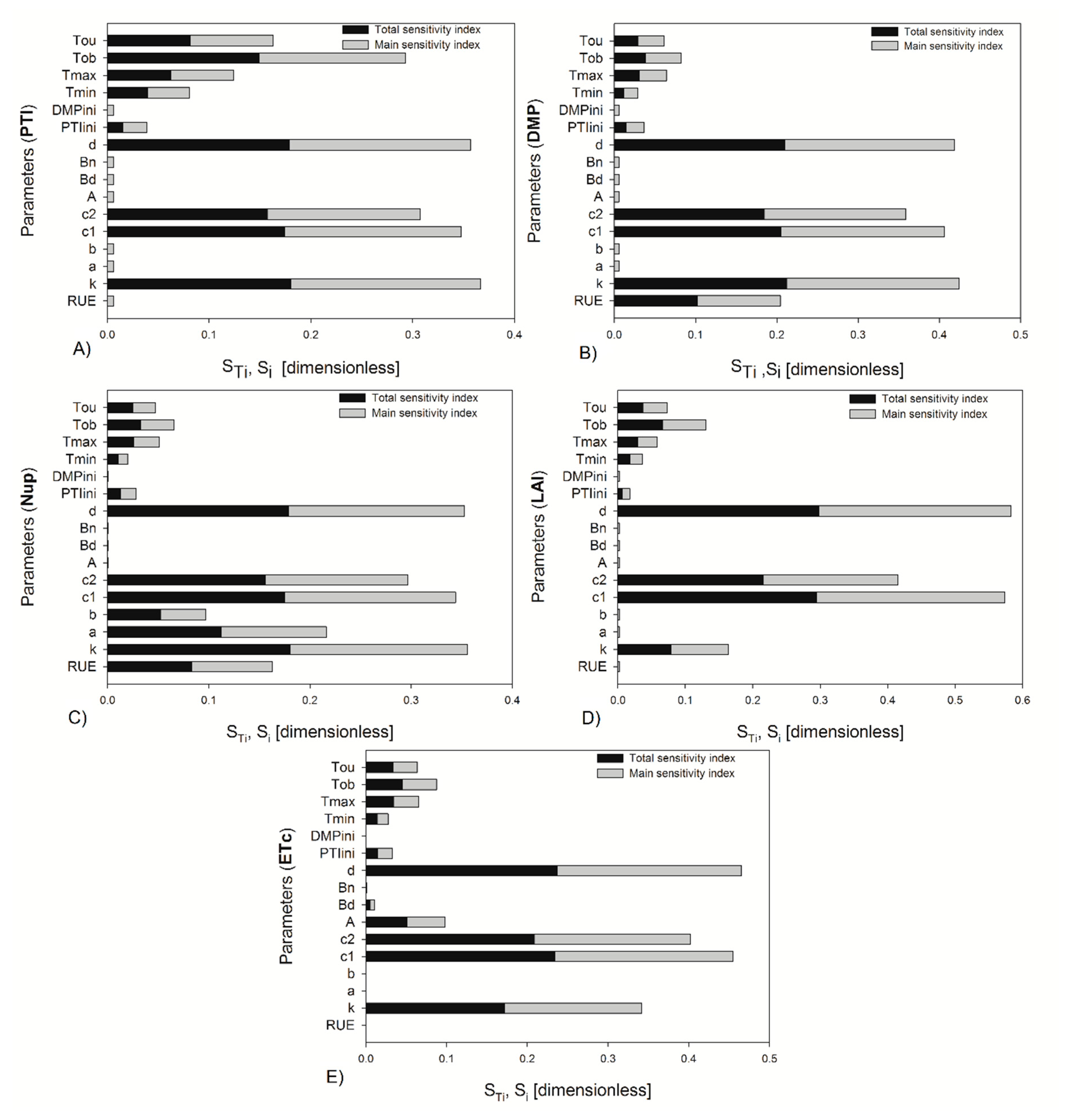
The global sensitivity analysis with Sobol’s method was carried out to select the parameters that are the most sensitive to the uncertainty of 10% and 20% applied to all parameters around their nominal values; the data of the climatic variables of the spring–summer season were used to run the simulations. To estimate the sensitivity indices for the HORTSYST crop model, the simulation was run 10,000 times at the start of fructification (40 days after transplant (DAT)) and at the end of the crop cycle (119 DAT).

The most influential parameters in the model are listed in

Table 4. Sensitivity of HORTSYST parameters in descending order of importance obtained with Sobol’s method applied to two tomato crop stages.

Output Response	At the Beginning of Fructification	At the End of Crop Growth
	Parameters (10% of variation)
PTI	${\mathrm{T}}_{\mathrm{ob}}$, ${\mathrm{c}}_1$, $\mathrm{d}$,$\mathrm{k}$, ${\mathrm{c}}_2$, ${\mathrm{T}}_{\mathrm{ou}}$	${\mathrm{T}}_{\mathrm{ob}}$, ${\mathrm{T}}_{\min }$
DMP	${\mathrm{c}}_1$, $\mathrm{d}$, $\mathrm{k}$, ${\mathrm{c}}_2$, $\mathrm{RUE}$	$\mathrm{RUE}$, ${ \mathrm{c}}_1$, $\mathrm{d}$, $\mathrm{k}$
Nup	$\mathrm{d}$, ${\mathrm{c}}_1$, ${\mathrm{c}}_2$, $\mathrm{k}$, $\mathrm{a}$, $\mathrm{RUE}$	$\mathrm{a}$, $\mathrm{b}$, $\mathrm{RUE}$
LAI	${\mathrm{c}}_1$, $\mathrm{d}$, ${\mathrm{c}}_2$, ${\mathrm{T}}_{\mathrm{ob}}$, $\mathrm{k}$	${\mathrm{c}}_1$, $\mathrm{d}$, ${\mathrm{c}}_2$
ETc	${\mathrm{c}}_1$,$\mathrm{d}$, ${\mathrm{c}}_2$,$\mathrm{k}$	${\mathrm{c}}_1$, $\mathrm{A}$, $\mathrm{d}$, ${\mathrm{c}}_2$, $\mathrm{k}$
	Parameters (20% of variation)
PTI	$\mathrm{k}$, $\mathrm{d}$, ${ \mathrm{c}}_1$, ${\mathrm{c}}_2$, ${\mathrm{T}}_{\mathrm{ob}}$, ${\mathrm{T}}_{\mathrm{ou}}$, ${\mathrm{T}}_{\max }$	${\mathrm{T}}_{\mathrm{ob}}$, ${\mathrm{T}}_{\min }$
DMP	$\mathrm{k}$, $\mathrm{d}$, ${\mathrm{c}}_1$, ${\mathrm{c}}_2$, $\mathrm{RUE}$	$\mathrm{RUE}$, ${ \mathrm{c}}_1$, $\mathrm{d}$, $\mathrm{k}$
Nup	$\mathrm{k}$, $\mathrm{d}$, ${\mathrm{c}}_1$, ${\mathrm{c}}_2$, $\mathrm{a}$, $\mathrm{RUE}$	$\mathrm{a}$, $\mathrm{b}$, $\mathrm{RUE}$
LAI	$\mathrm{d}$, ${\mathrm{c}}_1$,${ \mathrm{c}}_2$, $\mathrm{k}$, ${\mathrm{T}}_{\mathrm{ob}}$	$\mathrm{d}$, ${\mathrm{c}}_1$, ${\mathrm{c}}_2$
ETc	$\mathrm{d}$, ${\mathrm{c}}_1$,${ \mathrm{c}}_2$, $\mathrm{k}$	$\mathrm{d}$, ${\mathrm{c}}_1$, $\mathrm{A}$, ${\mathrm{c}}_2$,$\mathrm{k}$

. At 40 DAT, the sum of the first-order indices (main effects) for PTI was 0.95, and the sum of the total effect indices was 1.01; for the DMP variable, it was 1.00 for first-order indices, and the sum of total effect indices was 1.00; for Nup, it was 1.08 for first-order indices and 0.99 for the sum of total effect indices; for the LAI variable, 1.01 was obtained for first-order indices and the sum of total effect indices of 1.00; and finally, for ETc, 0.98 was for first-order indices and for the sum of total effect indices of 1.00. At 119 DAT, the sum of the first order for PTI was 0.96; for the DMP variable, the sum of this index was 0.92; for Nup, it was 0.99; for LAI, the value was 1.04; and for ETc, the sum was 0.93. The sum of the total effect indices for PTI was 1.00; for DMP, it was 1.02; for Nup, this sum was 1.01; for LAI, it was 0.99; and for ETc, the sum of these indices of 1.00 was found. In the fructification stage, the existence of interaction between parameters was not clear; however, for the second stage, such interaction was observed, since the values of the indexes $S_{Ti}>S_i$. 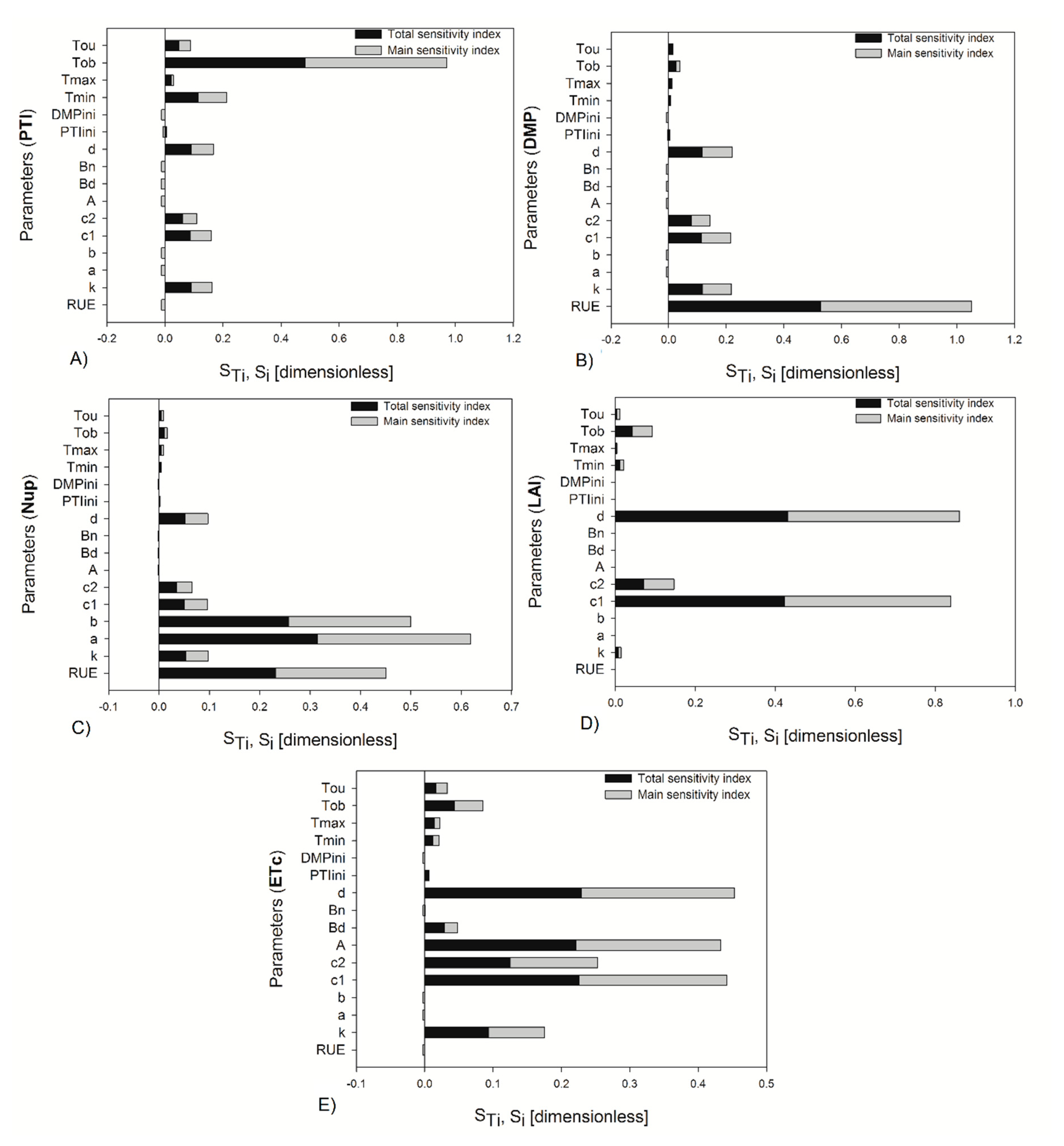Figure 2 and Figure 3 show the indices for 20% uncertainty on the parameters at the start of fructification and at the end of growth; in both cases the most important parameters were the same, with 10% uncertainty on the parameters. They only varied in order of importance, with these changes being the most evident for 40 DAT. The most important parameters in descending order are shown in Table 4. The sum of the first-order effects and the total indices were for PTI (1.08, 1.04), DMP (1.08, 1.04), Nup (0.99, 1.05), LAI (1.02, 1.05), and ETc (1.00, 1.06) at fructification stage. In the analysis performed with 20% uncertainty at 119 DAT, the parameter d (crop density) became more important than c₁ for ETc output, whereas the other parameters kept their order of importance found with 10% uncertainty. In the case of 119 DAT, the sum of the first-order effects and the total indices were for PTI (0.90, 1.00), DMP (0.91, 1.01), Nup (0.95, 1.02), LAI (0.99, 1.00), and ETc (0.96, 1.02).

The sum of total sensitivity indices for the most important parameters (${{\displaystyle \sum }}^{ }{S}_{Ti}$) was slightly higher than 1 when the sensitivity analysis was carried out with 10% uncertainty at 40 DAT and 119 DAT, but it is not conclusive to say that the model is nonadditive. Nevertheless, with the 20% uncertainty, the sums of total indices for all output responses for both crop stages were different from 1, so the model was nonadditive; this also was checked with the sum of the first-order effects $S_i$ < 1, according to Saltelli et al. [2]. The interactions between parameters were clearer when the uncertainty on the parameters was increased to 20% at the beginning of fructification and at the end of the crop cycle $S_{Ti}>S_i$ for all output variables.

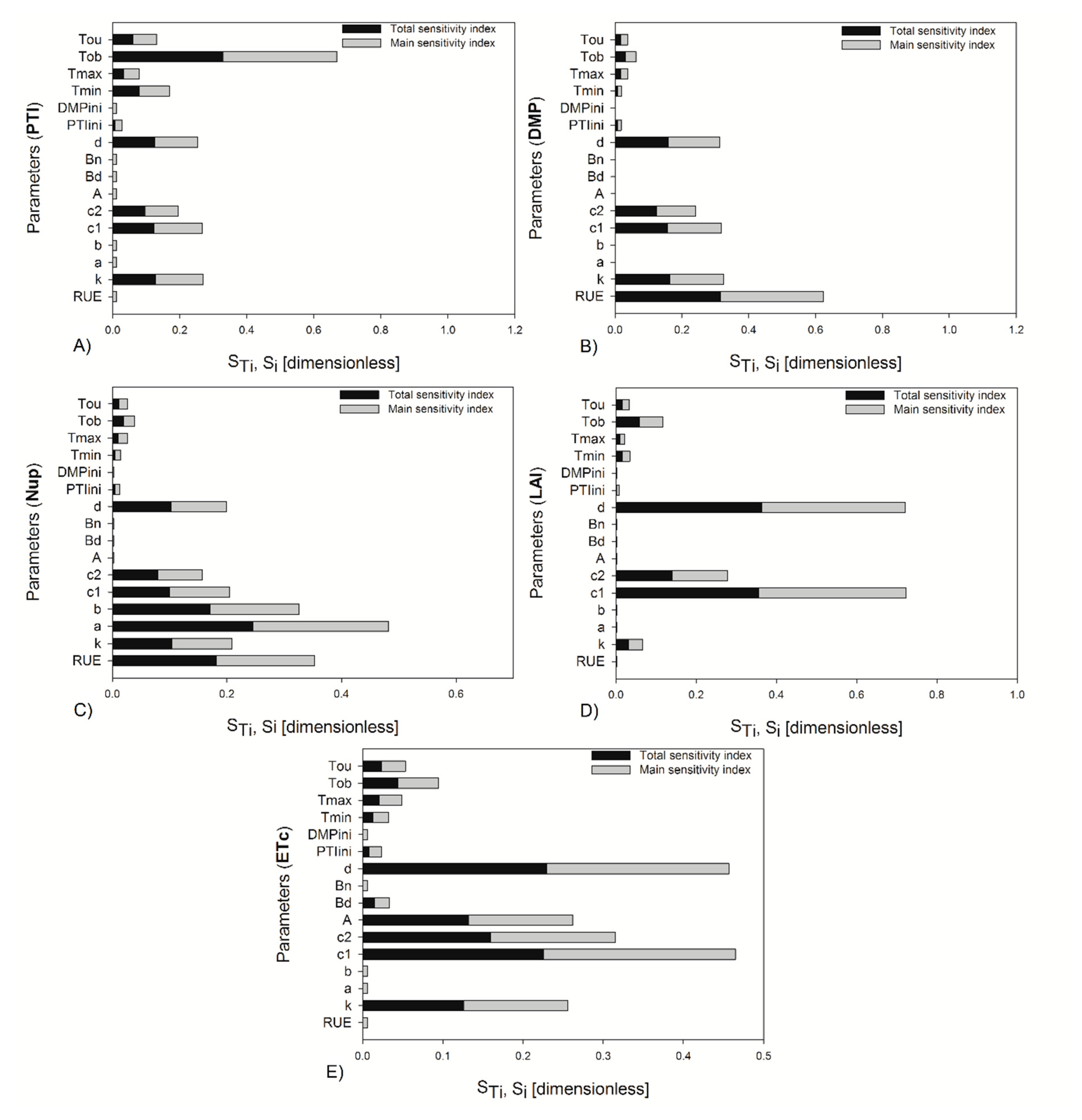
The sensitivity indices were also estimated, taking into account the daily integration of output variables at the end of the crop cycle with 20% uncertainty, and the indices found were different for some parameters than when two specific stages were considered in the analysis (Figure 4). For the daily integration of outputs, some parameters changed in their magnitude of importance; for example, for PTI and DMP, $T_{ob}$ and $RUE$ decreased their index values, and the rest of the parameters increased. The parameter $c_{2 }$ increased the magnitude of its indices for Nup, LAI, and ETc. In the sensitivity analysis run in the two growth stages, it was observed that a greater number of parameters were more important at the beginning of fructification than at the end of crop growth for 10% and 20% of the variation of the parameters (Table 4).

These results indicate that the parameters changed over time, with some of them increasing in importance and other decreasing; for example, the parameter $T_{ob}$ increased its importance in PTI, $RUE$ in DMP, $a$ and $b$ in Nup, $c_{1 }$ in LAI, and $A$ and $B_d$ in ETc. Two of the parameters that decreased their importance with the growth and development of the crop were $c_{2 }$(LAI, ETc, and DMP) and the parameter $k$. This temporal variation was also reported by López-Cruz et al. [52] with the NICOLET model for lettuce and the SUCROS model applied to husk tomato [53]. In addition, Wang et al. [54] found this variation throughout crop growth and the temporal dynamic variation as a result of the increase in uncertainty in the parameters of the WOFOST model used in corn cultivation.

The cardinal temperatures $T_{max}$, $T_{min}, T_{ob}$, and $T_{ou}$ had an influence on the model’s performance (Figure 2, Figure 3 and Figure 4), particularly at the beginning of fructification. However, these parameters were not selected for the parameter estimation technique, because they were taken from the literature [35,40,41]. All of these parameters were obtained by experimentation; other parameters, such as $k$ (extinction coefficient) and $d$ (crop density), were also not considered, though they showed high sensitivity in the analysis, because the $k$ parameter can be estimated with a ceptometer, and crop density ($d$) is defined before setting the experiment.

During the analysis, it was found that these two parameters were the most sensitive in all output variables of the model, since these output variables are strongly influenced by the interception of the light, which is dependent on the simulation of the dry matter produced, leaf area index area, and crop transpiration and indirectly dependent on the nutritional uptake, since its determination depends on the biomass produced by the crop.

The effects of these parameters were discussed by De Reffye et al. [33], who argued that limitations occur for light interception when density is low, because the expression of light interception assumes a homogeneous distribution of leaves. Therefore, the parameters that finally were considered for calibration were: $RUE$, $a$, $b$,$c_{1 }$,$c_2$,$A$, $B_d$, $B_n$, and $PTIini$. The $RUE$ parameter explains the quantity of carbon assimilated and converted to total dry biomass; thus, it was important for DMP and Nup, because the two variables are correlated. For models with the light-use efficiency approach, this parameter and $k$ become more significant, as was found for the CERES–maize model [55] and WOFOST model studied by Dzitsi et al. [56], the SALUS model for maize, peanut and cotton reported by Wang et al. [54], and AZODYN for wheat [57]; all of them found higher values of $S_{Ti}$ and $S_i$ for $RUE$, and $k$.

Parameters $a$ and $b$ are important for quantifying nitrogen uptake. The increase in the indices of these two parameters and $RUE$ from 40 DAT to the end of crop growth is explained by the increased slope of the exponential growth curve of total dry matter production due to the fruit’s filling, and this, in turn, increased crop nitrogen demand. $c_{1 }$ and $c_2$ explain the expansion of leaf area. The indices for $c_2$ decreased over time because the maximum LAI value of the crop was reached, meaning the plateau of this variable’s curve was attained; however, $c_{1 }$ increased its importance over time.

On the other hand, $A$, $B_d$, and $B_n$ influence the radiation and vapor pressure deficit (VPD) in the estimation of crop transpiration. The second and third parameters were not significant in this analysis. Similar results were found by Sánchez [58]. However, these authors found that these parameters become important for the autumn–winter season; for this reason, they were considered as significant parameters. The parameter $PTIini$ (one of the two initial conditions) did not have high values for $S_{Ti}$ and $S_i$, but we realized that it improved the performance of the calibration of the other selected parameters. The differences between two indices were for $RUE$ (0.004), $a$ (0.010), $b$ (0.015), $c_{1 }$ (0.004), $A$ (0.010), $\mathrm{and} B_d$ (0.01). The only parameters that did not have interaction were $c_2$, $PTIini$, and $B_n$.

3.2. Calibration of HORTSYST Model by Differential Evolution Algorithm

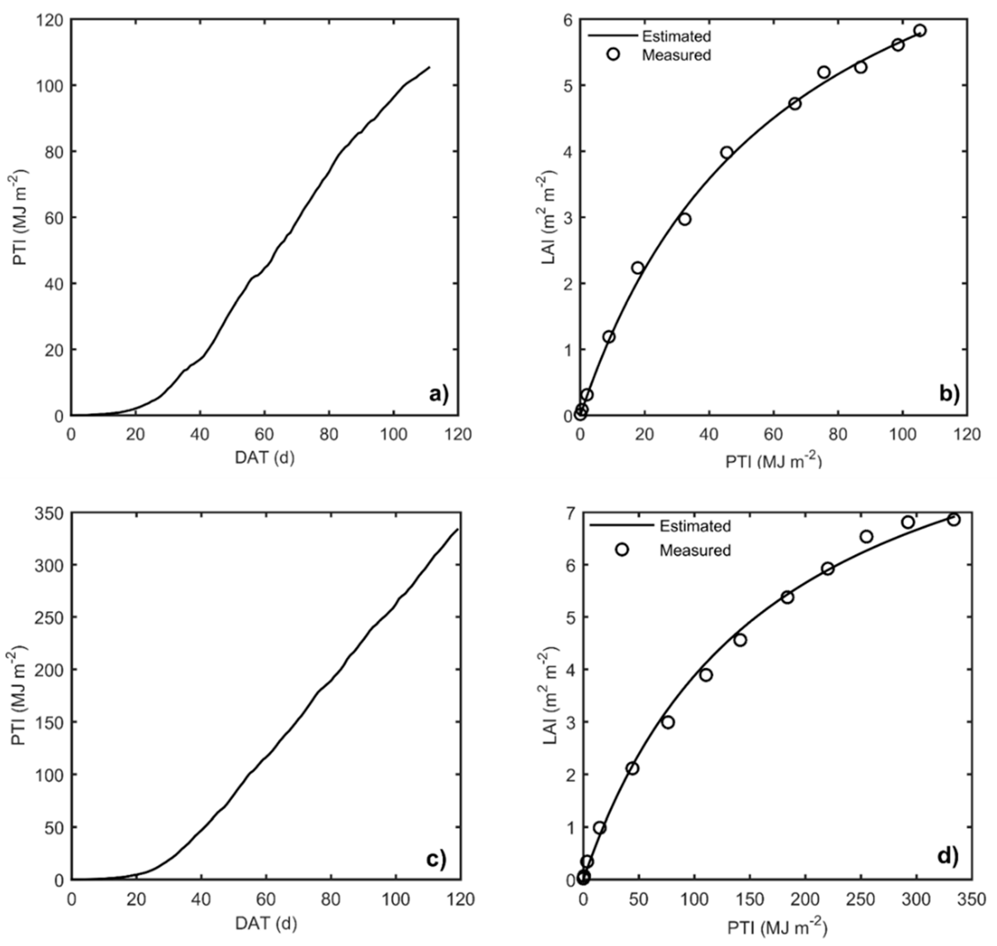
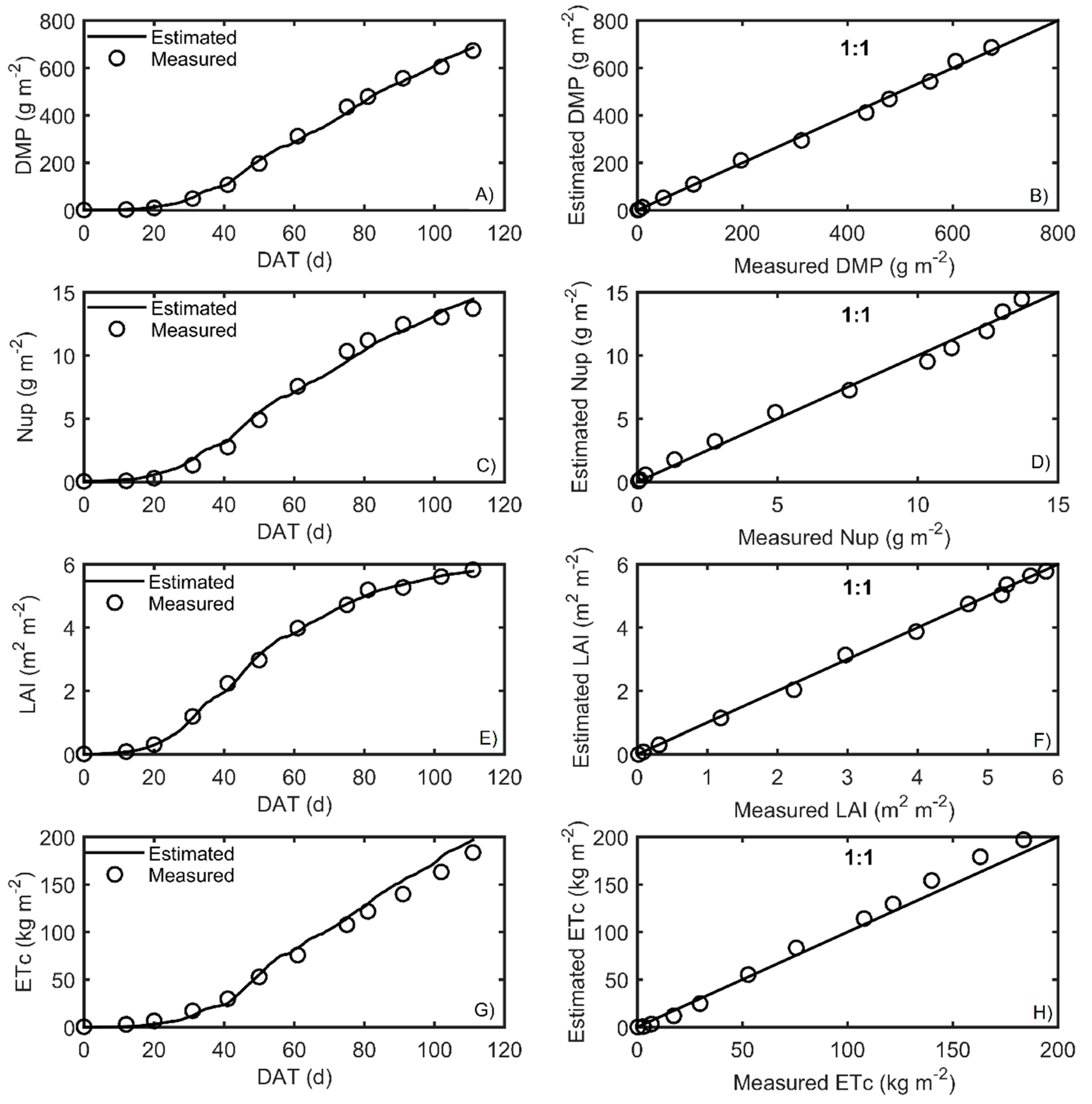
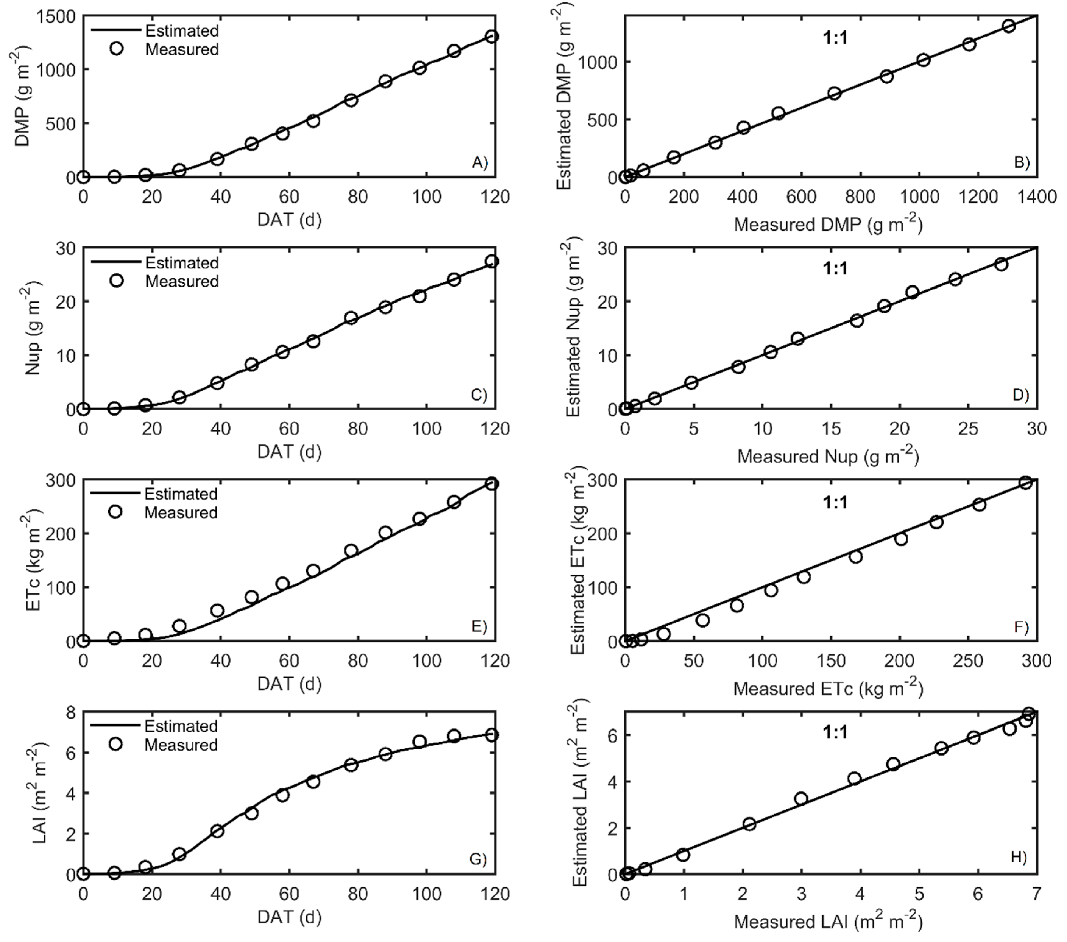
The HORTSYST crop growth model was calibrated by solving a minimization optimization problem. Nine parameters were estimated during the calibration for the autumn–winter and spring–summer seasons. PTI vs. LAI Michaelis–Menten function behavior after calibration are shown in Figure 5. Measured and simulated data after calibration are shown in Figure 6 and Figure 7. The values of the calibrated parameters are listed in Table 4, and the model’s goodness of fit statistics are presented in

Table 5. Parameter values and standard deviations after the differential evolution (DE) calibration process.

Parameters	Autumn–Winter		Spring–Summer
	Nominal Values	Standard Deviations	Nominal Values	Standard Deviations
PTIini	0.03	0.01 (2.05 × 10−9)	0.06	0.031 (4.58 × 10−9)
RUE	4.01	4.79 (3.81 × 10−7)	3.10	2.99 (2.10 × 10−7)
a	7.55	5.89 (1.23 × 10−5)	7.55	5.68 (7.34 × 10−6)
b	−0.15	−0.19 (4.06 × 10−7)	−0.15	−0.17 (2.23 × 10−7)
c1	2.82	2.65 (4.02 × 10−8)	3.07	2.97 (3.52 × 10−8)
c2	74.66	63.46 (1.26 × 10−9)	175.64	167.99 (8.85 × 10−13)
A	0.30	0.63 (4.58 × 10−9)	0.49	0.56 (2.40 × 10−9)
Bd	18.70	28.57 (1.99 × 10−7)	11.20	15.69 (2.18 × 10−7)
Bn	8.50	4.73 (4.45)	8.28	16.51 (6.13 × 10−7)

.

The best fits, according to RMSE, were for LAI, followed by Nup, DMP, and ETc for both crop seasons. The RMSE was close to zero, indicating an excellent prediction of model performance.

Another goodness fit index used to evaluate the model was the efficiency of the model (EF), which resulted in values close to one, which means that the model presented good adjustments when correlating the variables of the model, according to Xuan et al. [47] and Wallach et al. [51]. As for the bias values found in the autumn–winter season, the nitrogen uptake was slightly underestimated, and DMP, LAI, and ETc were overestimated; in the case of the spring–summer season, LAI and DMP were underestimated, and Nup and ETc were overestimated. Furthermore, the 1:1 plots are presented in Figure 6 and Figure 7 to visualize the quality of the prediction of the output responses in the HORTSYST model.

All parameters were accurately calibrated; only parameter $B_n$ in the transpiration rate turned out to have high standard deviation during the autumn–winter season (

Table 6. Goodness of fit statistics resulting from calibration of the model for autumn–winter and spring–summer.

Outputs	Autumn–Winter			Spring–Summer
	Bias	RMSE	EF	Bias	RMSE	EF
DMP	0.41566	13.3133	0.9970	−1.5437	14.7602	0.9989
Nup	−0.0708	0.5004	0.9909	0.0287	0.3583	0.9980
LAI	0.0249	0.0989	0.9979	−0.0007	0.1564	0.9962
ETc	3.6465	39.3297	0.8153	1.2918	28.2060	0.9581

). This means that it was very uncertain for autumn–winter, but this problem was not found for spring–summer. The calibrated $RUE$ value for autumn–winter was higher than that found by Gallardo et al. [30], and, for spring–summer, it was closer to what was reported by Challa and Bakker [42]; the values obtained from RUE were different for each crop cycle evaluated. The parameter $a$ was lower for the two crop periods, and $b$ was higher than reported by Gallardo et al. [30]; these calibrated values were quite similar for both seasons. For the LAI variable, the parameter $c_1$ was closer for two seasons, but $c_2$ during the spring–summer was more than twice that found in autumn–winter. The parameters $A$, $B_d$ concerning ETc were higher than those found by Sánchez et al. [43] for both the autumn–winter and spring–summer seasons. These parameters were different between each crop cycle.

The HORTSYST model’s parameters calibrated using the DE algorithm were closer than those found by Martinez-Ruiz et al. [21], who used a nonlinear least square method to find the correct values of the parameters for spring–summer, except for parameter $B_n$.

4. Conclusions

The global sensitivity analysis based on Sobol’s method was an effective procedure for determining the most influential parameters in the HORTSYST model. With this procedure to evaluate the sensitivity analysis, the number of parameters of the model were reduced from sixteen to nine; it was also realized that all parameters had a temporal variation in their sensitivity, which could be explained by each development stage of crop, since it is known that dry matter production, nitrogen uptake, leaf area index, and crop transpiration have nonlinear behavior.

The values found in the parameters during the calibration were the correct ones for the autumn–winter and spring–summer seasons, because the amount of radiation between the two crop seasons is different, and this was reflected in the dry matter production, nitrogen uptake, and crop transpiration. The parameter estimation was necessary for each crop period, because the climatic condition is different in the crop cycles. These parameter values could be used as reference values to simulate another crop grown in a greenhouse with nonlimitation of water and nutrients. However, more experiments are needed to validate this model using these estimated parameters, and more research is also needed to extend this model to another greenhouse × 10-grown crop.

The predictions of the model output variables during the calibration process were accurate, since the deviation or error between the simulated variables and the measurements was minimal. Therefore, the differential evolution (DE) technique used to estimate the parameters was effective and had good convergence, and its efficiency was computationally acceptable.

The HORTSYST model has a simple mathematical structure, and, due to the reduced number of influencing parameters (results of the sensitivity analysis) and its accurate prediction of the output variables during calibration and once validated, its implementation is feasible for irrigation and nutrient management in intensive crops, since it uses the RUE (radiation use efficiency) approach of some models mentioned above, which have been used as decision support systems (DSS) for the management of agricultural systems.