
The Impacts of Land-Use Input Conditions on Flow and Sediment Discharge in the Dakbla Watershed, Central Highlands of Vietnam


1
Graduate School of Environmental and Life Science, Okayama University, 3-1-1 Tsushima-naka, Kita-ku, Okayama 700-8530, Japan
2
Nong Lam University, Linh Trung Ward, Thu Duc District, Ho Chi Minh City 700000, Vietnam
*
Author to whom correspondence should be addressed.
Water 2021, 13(5), 627; https://doi.org/10.3390/w13050627
Submission received: 29 January 2021
/
Revised: 17 February 2021
/
Accepted: 24 February 2021
/
Published: 27 February 2021
(This article belongs to the Section Hydrology)
Abstract
:The main objective of this study was to evaluate various land-use input conditions in terms of the performance improvement found in consequent flow and sediment simulations. The soil and water assessment tool (SWAT) was applied to the Dakbla watershed from 2000 to 2018. After the calibration and validation processes, dissimilar effects between the input conditions on the flow and sediment simulations were confirmed. It was recognized that the impact of the land use on the sediment simulation was more sensitive than with the flow simulation. Additionally, through monthly evaluation, the effects against the flow and sediment in the rainy season were larger than those in the dry season, especially for sediment simulation in the last three months from October to December. Changing land-use conditions could improve flow and sediment simulation performance better than the performance found with static land-use conditions. Updated land-use inputs should be considered in simulations if the given land-use condition changes in a relatively short period because of frequent land-use policy changes by a local government.
1. Introduction
Changes in expanding hillslope cultivation, amplifying urbanization, and deforestation are some of the more notable issues in mountainous areas, particularly for countries in Southeast Asia. Areas with a transitional zone of forest and agricultural land experience the highest erosion caused by the encroachment of anthropogenic processes [1,2,3]. Additionally, excess discharge and rainfall intensity contribute to accelerating soil erosion and increase the sediment and nutrient losses to downstream [4,5].
In order to decrease erosion from the area and develop a sustainable land-use plan, the watershed basis approach has been recognized as an important method. Becaise land-use changes are the result of choices by local citizens/farmers, companies, and governments, information, such as (1) the suitable location of development/cultivation or protection in a watershed, (2) environmental influences of land-use changes, and (3) a balancing method of human activities and water/land conservation, is crucial when considering a watershed management strategy. The information can particularly assist local land-use decision-makers. At present, many methods, including paired catchment, statistical analysis, and hydrological modeling, have been utilized to assess the impacts of environmental changes on flow and sediment in a watershed scale [6,7,8,9].
The soil and water assessment tool (SWAT) has been widely applied for modeling watershed hydrology and simulating the movement of non-point-source pollution. In the existing studies on SWAT modeling, the impacts of land-use changes on runoff and sediment [10,11], water balances [12], hydrological processes [13], and streamflow characteristics [14] have already been analyzed by using a single static land-use input condition in different periods, confirming its capability. However, as with other simulation models, the simulation results are significantly impacted by the temporal and spatial distributions of all the input conditions, including topographic, land use, soil, and weather data [15]. Notably, the essential factor among these variables is the land-use input condition. Thus, the condition of a watershed with frequent land-use changes in a relatively short period cannot be evaluated appropriately by using a simulation model with a single land-use input condition. In another case, a delta approach is applied to analyze the impacts of land-use change in two periods using simulation results derived from different static land-use data. In such a case, the simulation results cannot comprehensively evaluate realistic land-use changes, meaning that strategic land-use planning would be difficult. Therefore, multiyear land-use input conditions in a model simulation improve the reproducibility of water components and sediment in the watershed.
Land-use update modules via linear interpolation among time stamps have been developed in SWAT, including SWAT2009_LUC [16], LUC-R script [17], and SWAT-LUT [18]. These modules are expected to provide realistic parameterization to incorporate different land-use categories in watersheds [18]. The advantages of using land-use update modules are based on the scale and intensity of land-use changes in terms of improving the spatial distribution responses and temporal predictions of the model [16]. Based on these approaches, many studies have emphasized the effects of land-use changes on soil and water resources [18,19,20,21], groundwater and surface runoff [16], water quality [22], and water components and sediment [23,24].
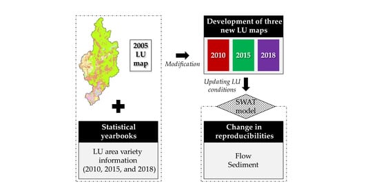
Thus, the main objectives of this study are (1) to create land-use maps following local statistical information in a watershed, where GIS-based information of land-use changes are infrequently updated while in the context of complicated local land-use policy changes, (2) to establish updated land-use input conditions by using the developed land-use maps, and then (3) to evaluate to what extent the updating land-use input conditions can improve the flow and sediment outputs of the model.
2. Materials and Methods
2.1. Study Area
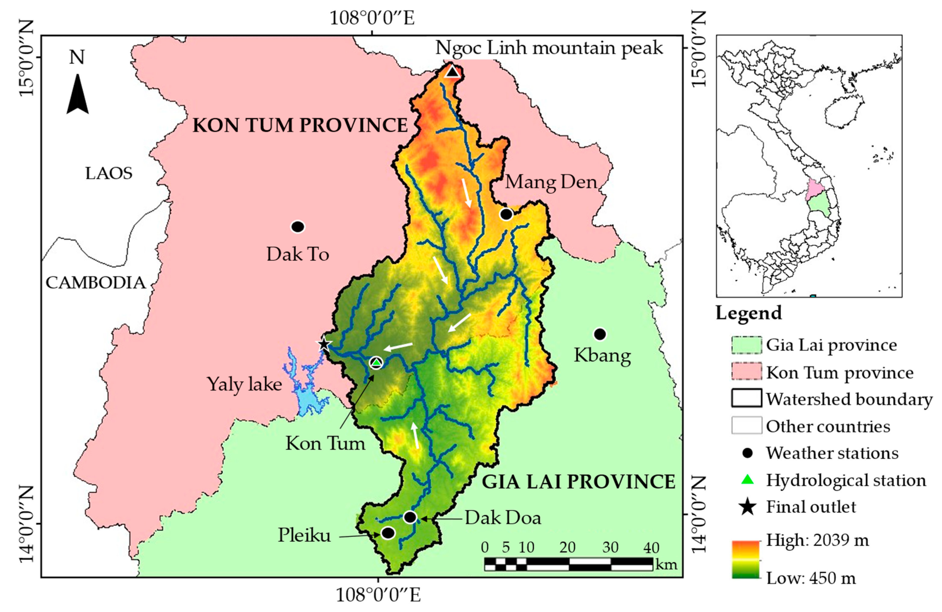
The Sesan River is one of the major tributaries of the lower Mekong basin in Southeast Asia. The Dakbla watershed, a subbasin of Sesan river basin, located in the Central Highlands of Vietnam with an area of about 3507 km2 (Figure 1). The total length of the main river is approximately 152 km. From the foot of Ngoc Linh Mountain (Tu Mo Rong District, Kon Tum Province), Dakbla River flows through the Kon Tum and Gia Lai Provinces in a northeast–southwest direction with a high drainage density of 0.49 km/km2. The river then flows to Yaly Lake in the downstream section after merging with the Poko River. The flow rates of the river are 0.2–0.5 m/s in the dry season and 1.5–3 m/s in the rainy season [25]. Being a mountainous area, the topography gradually decreases in the north–south and east–west directions. There are two principal seasons due to the tropical monsoon climate, including the rainy season (May to November) and the dry season (December to April). The average annual temperature is about 23.6 °C and the average annual rainfall is approximately 2000 mm at the Kon Tum weather station. More than half of the catchment area is covered in evergreen and mixed forests. With a proportion of 52%, clay loam is one of the most popular soil textures in the area.
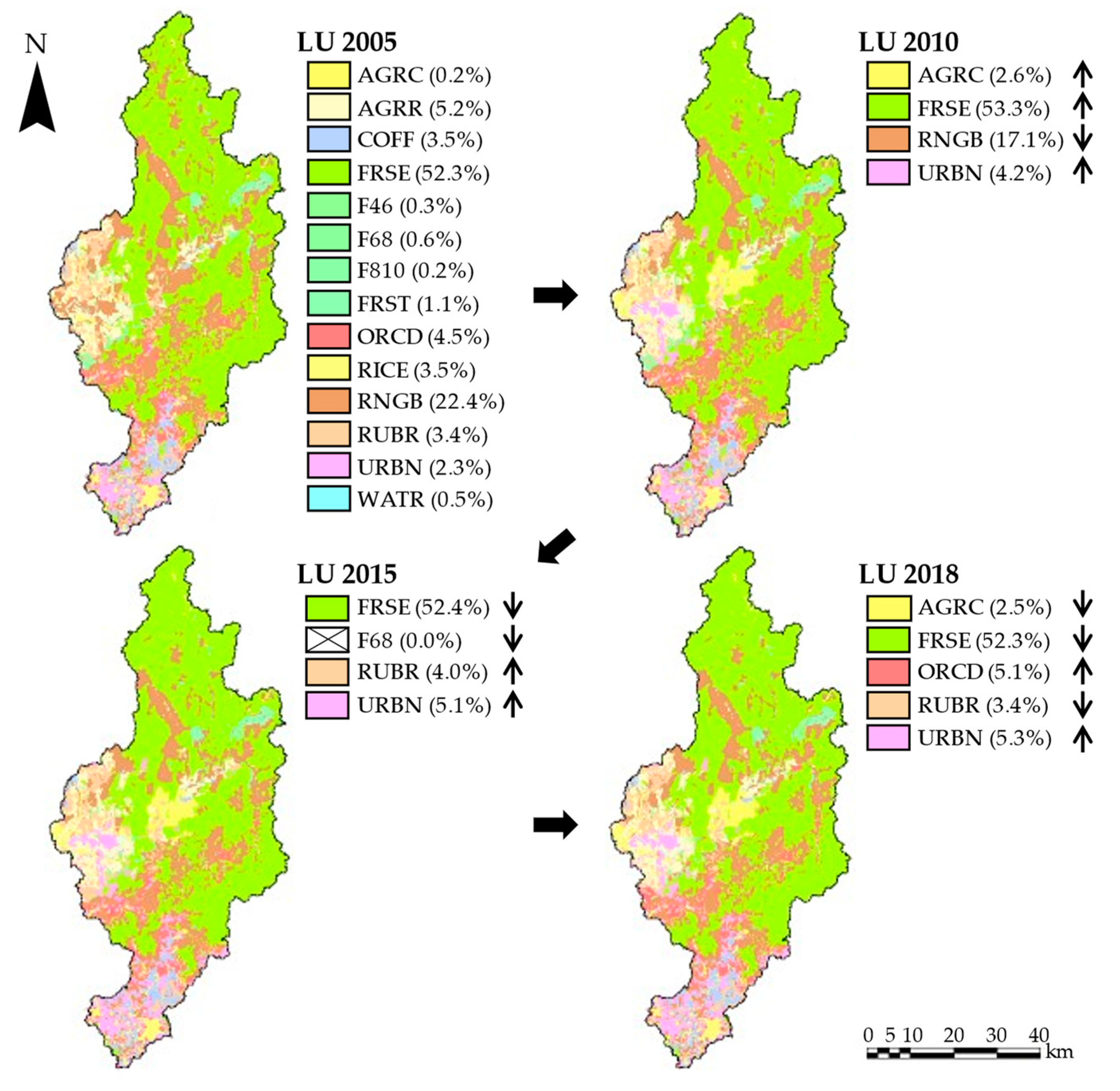
Rubber trees are considered to be plants that are suitable to the climatic and soil conditions in the Central Highlands of Vietnam. Since 2010, many projects have been conducted to convert mixed forests to rubber forests to create jobs and generate income for local people, especially ethnic minorities [26]; however, most of the new rubber trees have not grown in Gia Lai Province after two or three years of planting because they have been planted on dipterocarp forestland with low fertility, a thin arable soil layer, and poor organic compounds. To solve these obstacles, the conversion of inefficient rubber areas to other crops has been conducted in Gia Lai Province from 2015 onwards. As can be seen clearly in the statistical yearbooks published from the local government, the policies for land-use categories change dramatically every year, and these changes have been confirmed by the information for land-use change percentages; however, land-use maps have not been developed after the rapid changes in 2005. Thus, no spatial GIS information is available for after 2005 in the study area.
2.2. Input Data
The SWAT model requires spatial data (digital elevation model, land-use map, and soil map) and meteorological data (rainfall, maximum and minimum air temperature, relative humidity, wind speed, and solar radiation) as inputs.
The digital elevation model (DEM) was downloaded from the NASA and Japan ASTER Program [27] with a resolution of 30 m. The range of the topographic elevation in the study area varies from 450 m to 2039 m.
Land-use data were obtained from the Department of Environment and Natural Resources for the Kon Tum and Gia Lai provinces with a 1:50,000 scale map that was created using the information from 2005. Forestry land makes up the highest percentage with a value of 52.3%, and mixed forests occupy only 2.2%. Orchard, coffee, rubber trees, and agricultural land row crops occupy 16.6% in the total area. The remaining areas are rangelands, water areas, urban areas, and other types, in which rangeland accounts for 22.4% of the whole catchment.
Soil data were obtained from the Department of Environment and Natural Resources in Gia Lai Province and the Department of Information and Communication in Kon Tum Province with two 1:50,000 scale maps. Soil types were categorized into six groups based on soil textures, in which clay loam and clay were two popular soil textures with a combined proportion of 82.9%. The remaining parts account for negligible amounts, including loam, loamy sand, sand, and sandy clay.
Weather data were provided by the Central Highland Region Hydrometeorological Centre. The Kon Tum (Kon Tum Province) and Pleiku (Gia Lai Province) are weather stations with rainfall, minimum and maximum temperature, humidity, sunshine hours, and windspeed data from 1990 to 2018. Solar radiation was calculated with the Angstrom formula by utilizing the sunshine hour data for this area [28]. Four other stations, including the Dak To, Dak Doa, Kbang, and Mang Den weather stations, provided daily rainfall data. Dak to weather station also provided temperature data.
River discharge and total suspended sediment (TSS) concentration were recorded at Kon Tum hydrological station by the Department of Environment and Natural Resources in Kon Tum Province from 2000 to 2018. The summary of the flow and TSS data are shown in Table 1.
2.3. Methods
2.3.1. Brief Description of SWAT
SWAT is known as a physically based semi-distributed hydrological model that was developed by the Blackland Research and Extension Center and the Agricultural Research Service of the United States Department of Agriculture (USDA-ARS). This focused on predicting the impacts of land management practices on water and sediment in large complex watersheds over long periods of time [29]. There are many papers that have used this hydrological model to simulate water discharge and base flow [30,31,32], as well as sediment for specific storm events [33]. This model has also been used to show the relationships between sediment, rainfall, and simulated surface runoff [34,35]. By using this model, the impacts of land-use changes have also been analyzed in terms of annual hydrological components and sediment [16], as well as flow, total nitrogen, and total phosphorus loads [20]. The above evidence reveals the reliability and wide applicability for the model, especially in mountainous areas.
Simulation of hydrology is based on the water balance equation, as shown in Equation (1):
where : the final soil–water content (mm H2O); : the initial soil–water content (mm H2O); : the time (day); : the amount of rainfall on day i (mm H2O); : the amount of surface runoff on day i (mm H2O); : the amount of evapotranspiration on day i (mm H2O); : the amount of percolation and bypass flow exiting the soil profile bottom on day i (mm H2O); and : the amount of return flow on day i (mm H2O).
In addition, erosion caused by rainfall and runoff is computed with the Modified Universal Soil Loss Equation (MUSLE) in SWAT [36]. To predict sediment loss, the peak runoff rate is used. Erosion and sediment yields are calculated for each hydrological response unit (HRU) by using Equation (2):
where : the sediment yield on a given day (metric tons); : the surface-runoff volume (mm H2O/ha); : the peak runoff rate (m3/s); : the area of the HRU (ha); : the USLE soil erodibility factor (0.013 metric ton m2 hr/(m3-metric ton cm)); : the USLE cover and management factor; : the USLE support practice factor; : the USLE topographic factor; and : the coarse fragment factor.
2.3.2. SWAT Application
To evaluate model output accuracy, daily observed runoff and sediment data were utilized. The watershed was divided into 73 subbasins in the model. The SWAT parameter values were calibrated for 10 years from 2000 to 2009 and validated for another 9 years from 2010 to 2018. The most sensitive 13 parameters were calibrated, such as CN2 (SCS runoff curve number), SURLAG (surface-runoff lag time), SOL_AWC (available water capacity of the soil layer), SOL_K (saturated hydraulic conductivity), USLE_P (USLE support practice factor), ALPHA_BF (baseflow alpha factor), and GW_DELAY (groundwater delay), in order to improve the model performance. The calibration of the parameter values was conducted using the SUFI-2 algorithm in the calibration uncertainty program for SWAT (SWAT-CUP) [37].
2.3.3. Land-Use Change Update Module
The land-use change modules were developed for SWAT via SWAT2009_LUC [16], SWAT-LUT [18], or scripting with R [17], which is a free software package for statistical computing and graphics developed by the R Foundation for Statistical Computing [38]. The software enables updated land-use changes to be considered in the SWAT model by linear interpolation at the chosen time. With many approaches, land-use changes with time stamps are simulated, while other factors remain stable [18].
2.3.4. Preparation of Land-use Maps in 2010, 2015 and 2018 and Land-use Scenario Settings
In the traditional SWAT applications, only a single land-use map is utilized to simulate target elements for a whole target period. In this study, a 2005 land-use map was used as the base land-use map for the simulation; however, as many land-use policies have been implemented since 2010 by the local government, the 2005 land-use map was updated with the information from the statistical yearbook recording data, such as the area for each land-use category and the crop varieties in each province. Based on local policy decisions for land uses and the statistical information, new land-use maps were developed for 2010, 2015, and 2018 (Figure 2). As only statistical information was available and there was no spatial location information for the land-use changes after 2005, historical local information was employed, which mentioned that mixed forests have been converted to rubber forests in the altitude range from 600 to 800 m. This knowledge was used to update the hypothetical land-use percentages. Specifically, by using the DEM information, the mixed forest area was further divided into three categories from 400–600 m, 600–800 m, and 800–1000 m, and mixed forest land use was updated for a 600–800 m altitude to fit the conversion percentages in the statistical yearbooks for the district data. The percentages of other land-use categories in the 2010, 2015, and 2018 land-use maps were also changed to fit the statistical information from the district level without considering altitude.
In the 2010 statistical yearbook, the agricultural, forest, and urban areas increased by 8.4, 1.8, and 27.1%, respectively, whereas rangeland decreased by 12.4% in the watershed compared to 2005. This meant that afforestation, agricultural expansion, and urbanization were conducted until 2010, mainly in the northern, western, and northwestern areas. After 2010, crop conversion was conducted in the target area. As mixed forests in the area had been exhaustedly exploited, they were no longer able to provide timber products [39]. Moreover, there was a decreasing tendency for rubber trees from 2010 till 2014 [40] as new rubber trees had not grown in Gia Lai Province after two or three years after planting. The combined rubber tree area for the five districts in Kon Tum Province was 4439 ha, accounting for approximately 21.5% of the total mixed forest area (20,692 ha) [41], and the rubber tree area was 23.7% in Gia Lai Province (11,385 ha of rubber trees of the total 47,943 ha in the mixed forest) [40].
In the 2015 statistical yearbook, the urban area increased continuously in the southern region with a value of 14%, while there was a decrease of forestry land by approximately 3.4% in contrast to 2010. Following the policy changes, conversion from inefficient rubber areas to other crops in Gia Lai Province was conducted. The other crops included orchard trees, agricultural crops, and industrial crops [42]. From 2015 onwards, based on the statistical yearbooks, the orchard areas increased by 3.8% and 56.3% in the provinces of Kon Tum and Gia Lai, respectively. At this moment, the detailed spatial areas of rubber trees converted to orchards were unknown in both provinces.
In the 2018 statistical yearbook, the urban area increased continuously with a value of 1.7%, while there was a decreasing tendency for agricultural land and forestland with values of approximately 0.3% and 0.6%, respectively, compared to 2015.
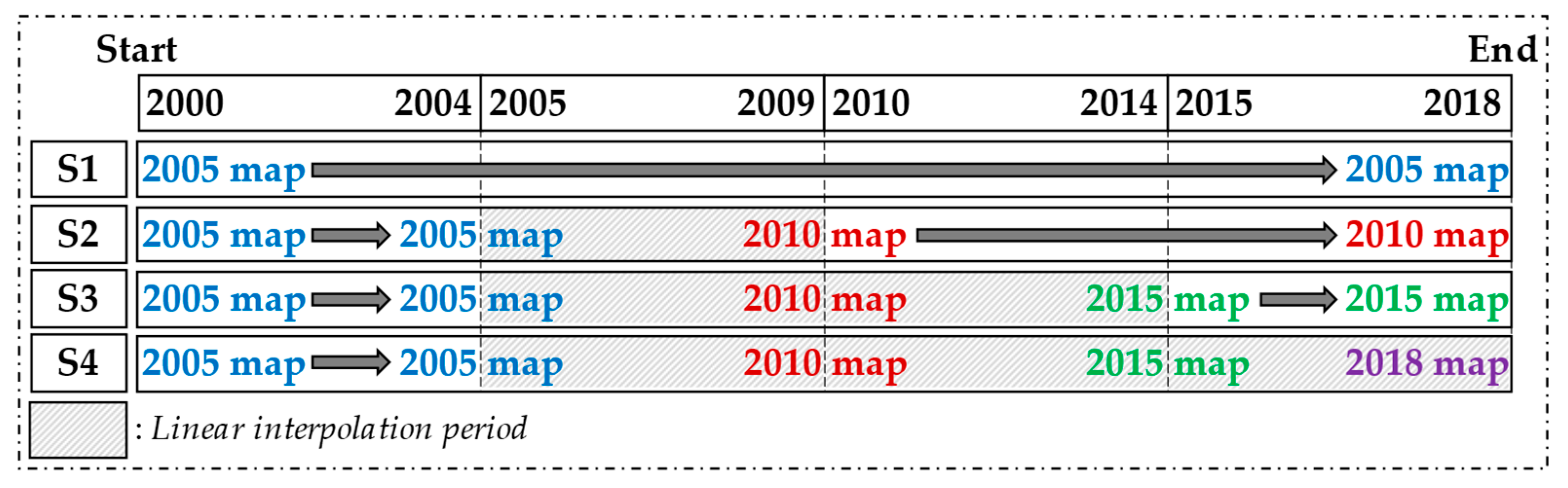
Four land-use scenarios were considered, including one static input condition with the 2005 land-use map (S1) and three updated input conditions (S2, S3, and S4) in the simulation (Figure 3). In S2, S3, and S4, the 2005 land-use map was utilized during the 2000–2004 period of simulation. In S2, the developed 2010 land-use map was used for the 2005–2018 period of simulation. For S3, the 2010 and 2015 land-use maps were utilized in the 2005–2009 and 2010–2018 simulation periods, respectively. In S4, the 2010, 2015, and 2018 land-use maps were utilized in the 2005–2009, 2010–2014, and 2015–2018 simulation periods, respectively. The weather input data between the four scenarios were the same.
2.3.5. Model Performance Evaluation
Each statistical index has advantages and disadvantages, and it is appropriate to utilize multiple parameters to evaluate the model performance more comprehensively [43]. In this study, to evaluate the accuracy of the SWAT model outputs, the coefficient of determination (R2), the Nash–Sutcliffe index (NSI), and the percent bias (PBIAS) were used, as shown in Equations (3)–(5):
where is the observed discharge, is the average observed discharge, is the simulated discharge, is the average simulated discharge, and n is the number of registered data.
R2 demonstrates the combined dispersion against the single dispersion of the observed and predicted values [44]. NSI indicates how well the plot of the observed values versus the simulated values fits the unit slope line [45]. Values greater than 0.5 for these variables are considered acceptable. If NSI ≥ 0.65, the simulation of model is considered extremely good [44,46]. PBIAS represents the average trend of the simulated values to be more different than their observed counterparts. The optimal value is 0, and positive and negative values indicate a bias toward underestimation and overestimation, respectively [47]. If the PBIAS value is between –10% and 15% for monthly flow and between ±10% to ±20% for sediment, this means that the model simulation can be judged as satisfactory [43].
2.3.6. Uncertainty Analysis Method
The output uncertainty after updating the land-use change was evaluated using the relative difference (RD) indicator, which illustrates the percentage error compared to the base data, as shown in Equation (6):
where Di is the model output using the updated land-use input conditions (S2, S3, or S4), and Si is the model output while using the static land-use input condition (S1).
3. Results
3.1. Reproducibility of Flow and Sediment in the Calibration Period (2000–2009)
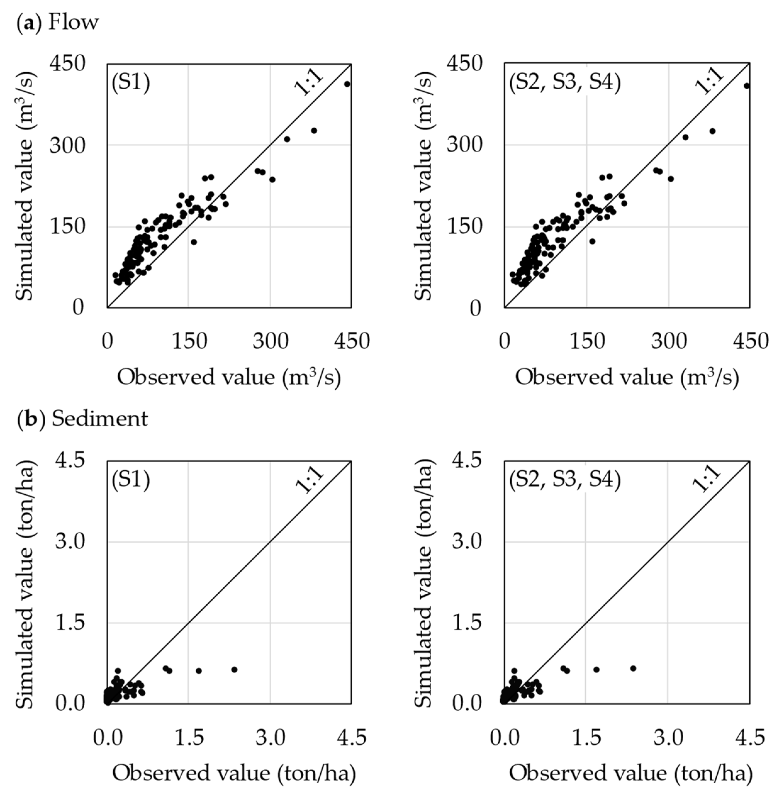
The flow was simulated with R2, NSI, and PBIAS values of 0.78, 0.70, and –8.1%, respectively (Table 2). Most of the values lay around the 1:1 line shown in Figure 4. There were some special cases with some underestimated peaks, leading to fluctuation of the statistical parameters. During this period, for example, enormous historical flooding occurred on September 29th in 2009, where the observed water discharge at Kon Tum hydrological station was 3500 m3/s with a corresponding rainfall value of 152.4 mm at that time.
As for the sediment, the results showed that the flow simulation of the model was better than that with the sediment simulation. The reproducibility of the model was evaluated with R2, NSI, and PBIAS values of 0.74, 0.66, and 31.5% in the calibration period.
The simulated results for both flow and sediment were evaluated to be between “very good” and “satisfactory” in the period from 2000 to 2009, except for the PBIAS for sediment.
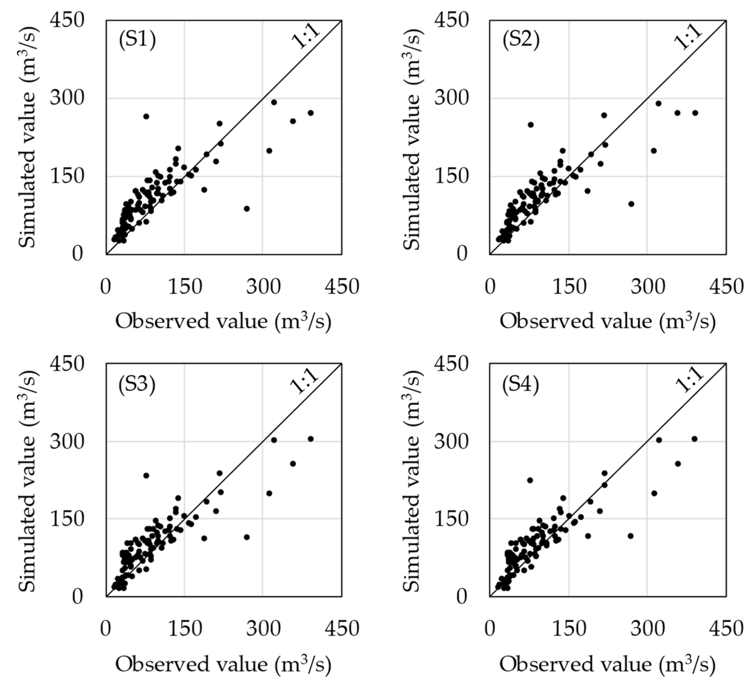
3.2. The Influence of Land-Use Update on Flow in the Validation Period (2010–2018)
The validation result for the static land- use condition (S1) was lower than that with the calibration because some values were scattered around the 1:1 line (Figure 5). During the 2010–2018 period, there was flooding on October 19, 2011, with flow and rainfall values of 1000 m3/s and 57.4 mm, respectively. The reproducibility between the observed and simulated flow in S1 was evaluated as satisfactory, which was represented by R2 = 0.68, NSI = 0.62, and PBIAS = –14.6%. As can be seen, the SWAT could accurately simulate flow and sediment in the target watershed. Thus, the calibrated and validated parameter values were utilized for the simulation with three updated land- use conditions.
The performance of the model when using the updated land- use scenarios was improved when compared with the S1 result for flow in the validation period. The NSI values for S2, S3, and S4 were 0.64, 0.65, and 0.65, respectively, which were slightly higher than that found with S1. The flow values tend to be closer to the 1:1 line. The R2 values were 0.68, 0.70, and 0.70, and the PBIAS values were –16.3%, –8.0%, and –7.4%, for S2, S3, and S4, respectively. As a result, S4 had the highest accuracy of the models in terms of flow simulation.
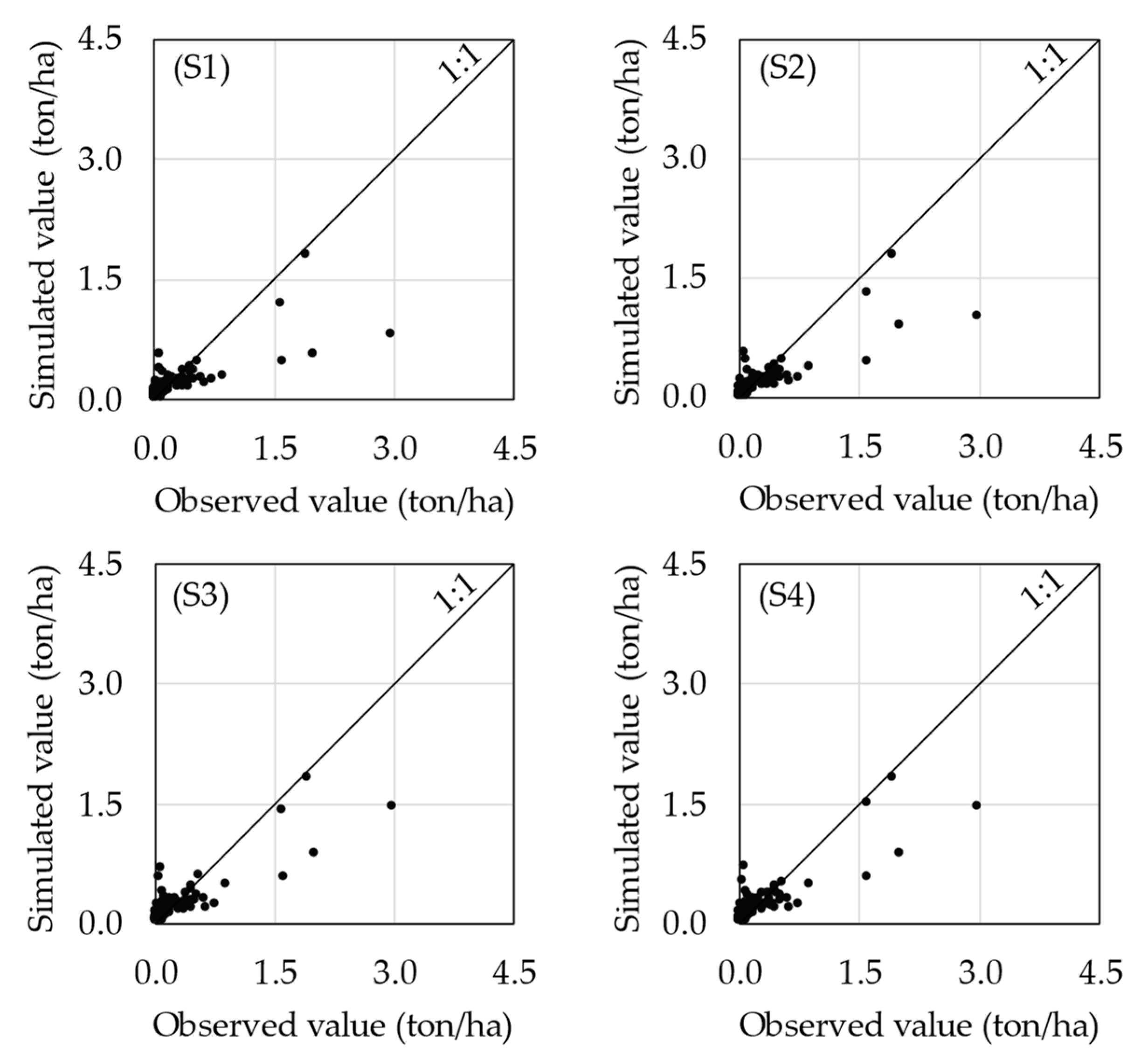
3.3. The Influence of Land-Use Update on Sediment in the Validation Period (2010–2018)
Similar to the flow simulation, the validation result for S1 found the lowest R2 and NSI values between the four scenarios as some values were scattered around the 1:1 line (Figure 6). This was caused by some underestimated sediment peaks, leading to the lower accuracy of the model. In S1, the correlation between the observed and simulated sediment values was within the satisfactory threshold with R2 = 0.63, NSI = 0.54, and PBIAS = 18.4%. Focused on the three updated land- use scenarios, the NSI values were higher than S1, in which S3 and S4 both produced the highest NSI value of 0.62, and a lower value of 0.55 for S2. With S3 and S4, the PBIAS value for S4 was better than S3, although they had similar NSI values. The observed sediment data had some enormous peaks, which might be related to a limitation of the sediment measurement.
Through evaluation of the flow and sediment reproducibility by using the three statistical values, the target elements were found to be well simulated for both the calibration and validation periods for S1 and the updated land- use scenarios (S2, S3, and S4). As for the flow simulation, the validated results slightly changed for the updated land- use scenarios compared to S1. Nevertheless, for sediment, the updated land- use input scenarios improved the model performance, especially S4, which considered the local land- use change policies. The NSI index reached a value of 0.62 for S4 instead of 0.54 in S1. Between the different land- use input scenarios, S4 seems to be the best scenario for both the flow and sediment simulations.
3.4. The Responses of Flow and Sediment to the Different Land-Use Input Conditions
For surface runoff, groundwater, water yields, and evapotranspiration, the RD values did not change much between the updated land-use scenarios and S1 (Table 3). There was a decrease for S2 with a value of 2.5%, whereas surface runoff in S3 and S4 increased by 5.1% and 5.2%, respectively. The RD values for groundwater did not exceed 1.5% between the different scenarios compared to S1. For water yield and evapotranspiration, the differences in S2 were higher than those in S3 and S4 when compared to S1, where there were moderate decreases with values of 1.7% and 5.3%, respectively, and these values changed slightly by only less than 2% for S3 and S4; however, the sediment yield changes were relatively large for S2 (–24.3%), S3 (25.7%), and S4 (27.1%). Particularly, the highest value of sediment yield reached 8.9 tons/ha for S4, and the RD value increased dramatically by approximately 27.1%. In S2, there was a reverse tendency with a significant 24.3% RD value. The higher uncertainty of sediment was caused by the fluctuation of sediment peaks. Overall, the simulation of sediment under the land- use input conditions was affected more than the other components.
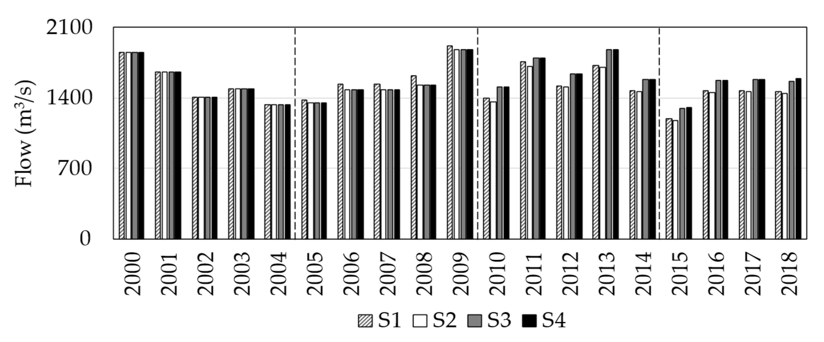
On an annual basis, compared with S1, the updated land- use input scenarios slightly changed the annual flow. S2, S3, and S4 reached lower values than S1, and the RD values ranged from 0.1% to 8.9%. During the 2000–2018 period, the highest total annual flow for S1 remained the same with 1918 m3/s in 2009, and there were decreasing trends of 2.2% for the three other scenarios in 2009. The lowest value for S1 was 1196 m3/s in 2015 (Figure 7). Compared to S1, S2 had a slight decrease of 1.4%, whereas there were moderate rises of 8.6% and 9.5% for S3 and S4, respectively.
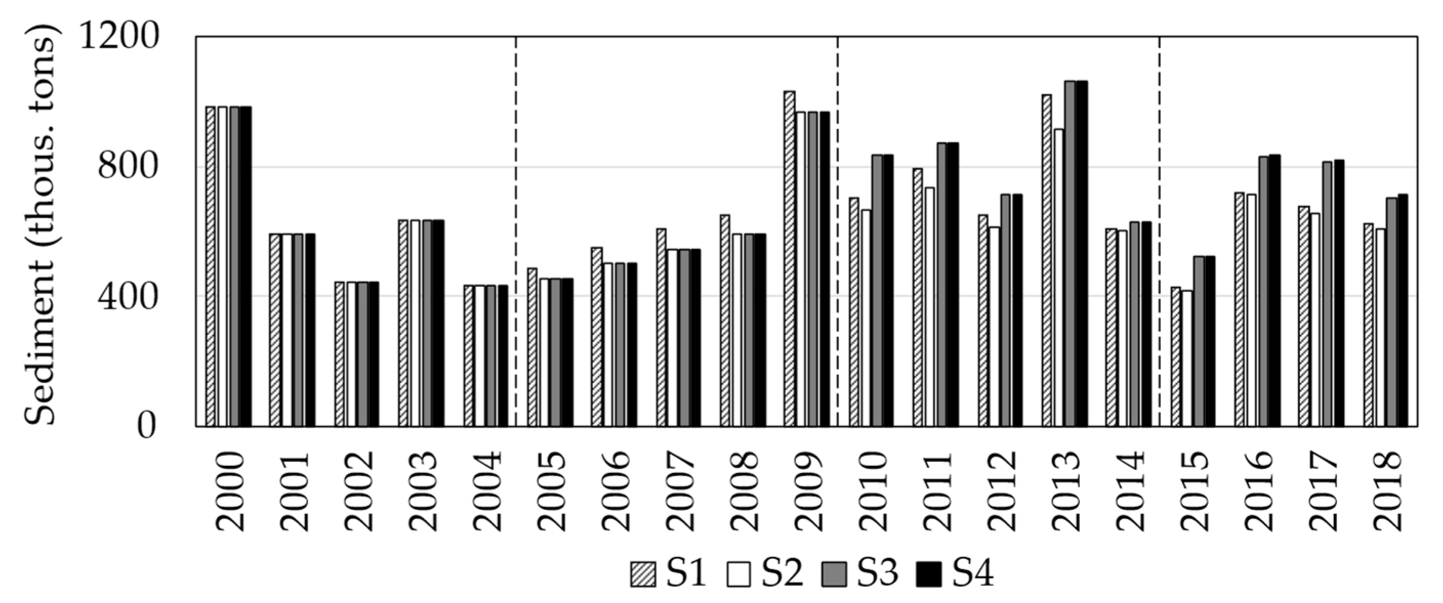
The total annual sediments had larger changes than those for the flow values under different land- use input conditions, especially throughout a 2015–2018 period (Figure 8). In the whole simulation period, S1 reached the highest sediment values of 1028 thousand tons in 2009, and then the value decreased by 5.8% in the others. The value in 2015 was the lowest in S1, and then the value decreased slightly by 2.0% in S2 and increased significantly in S3 and S4 by approximately 22.0% and 22.4%, respectively.
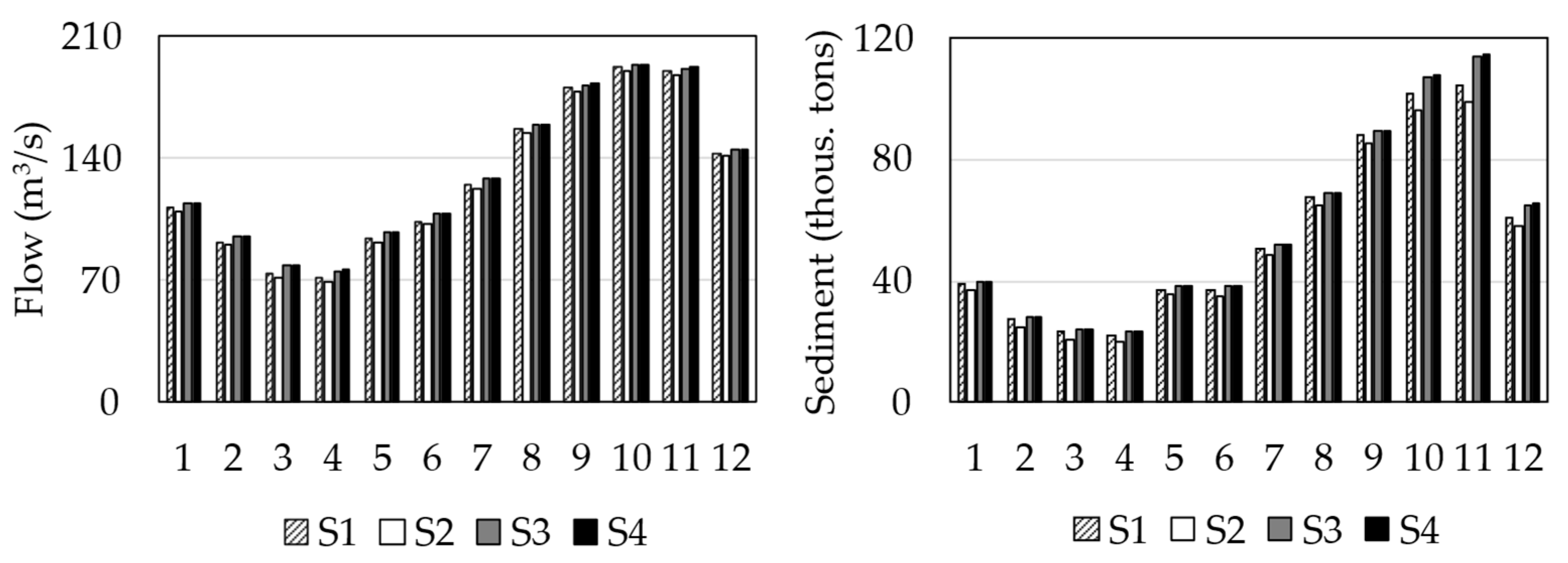
On a monthly basis, the highest values for all scenarios occurred in October for runoff and November for sediment (Figure 9). The RD values for the monthly flow did not exceed 3.2% for S2, 6.2% for S3, and 6.3% for S4. The highest flow value in S1 was approximately 192.3 m3/s in October. S2 had a slight decrease of only 1.0%, whereas there were increasing trends with 1.0% and 1.1% for S3 and S4, respectively. Oppositely, a larger change was observed for the sediment values with the updated land- use scenarios. The RD values for monthly sediment reached 7.0% in S2, 9.4% in S3, and 9.7% in S4. The highest value in S1 was 104.6 thousand tons in November, and there were increasing tendencies of 9.2% and 9.7% for S3 and S4, while there was a decreasing tendency of an approximately 5.1% for S2 when compared with S1. The last three months, including October, November, and December, featured significant changes during the year.
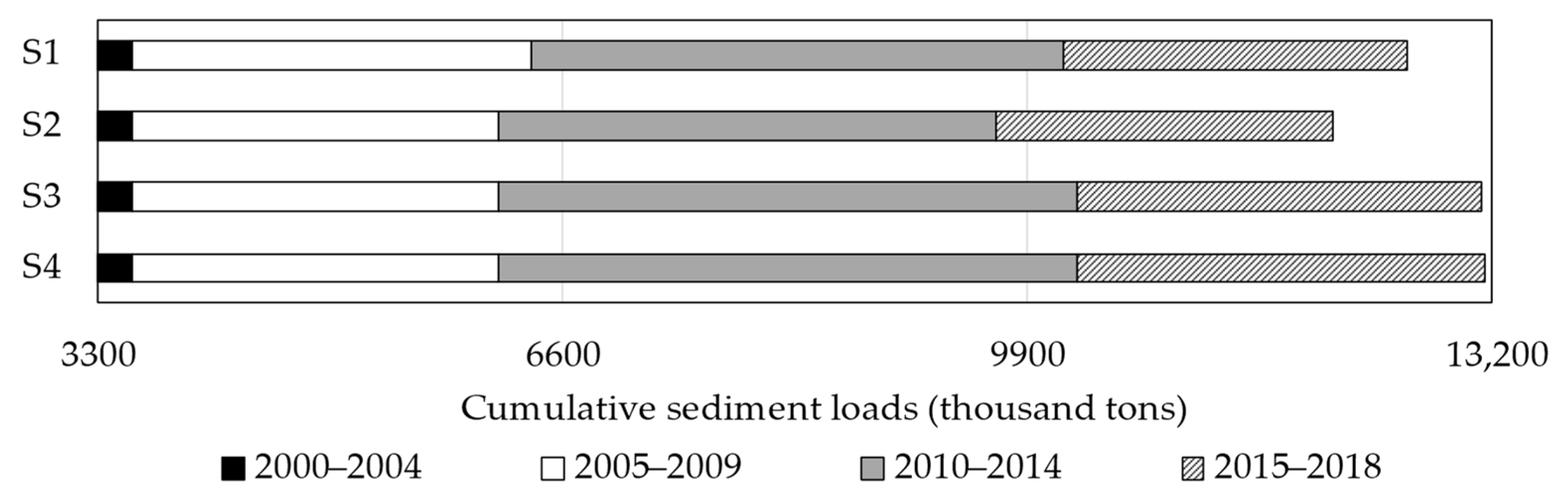
As the number of loads discharging from the watershed to downstream were affected by the land-use management history, the differences in the cumulative sediment loads from 2000 to 2018 were compared between the different land- use input conditions. Significant differences were found to exist between the four scenarios at the end of the simulation (Figure 10). During the 2000–2004 period, where the same land- use map was used in all scenarios, the sediment loads were all 3540 thousand tons. After 2005, where S2, S3, and S4 used the updated land- use information in the simulation, the cumulative sediment loads during 2005 to 2009 were slightly lower than those in S1, where they decreased by 232 thousand tons, corresponding to 0.8 tons/ha. After 2010, S3 and S4 used updated land- use information in the simulation, where the cumulative sediment loads during 2010 to 2014 changed from 3772 thousand tons in S1 to 3526 thousand tons in S2, 4105 thousand tons in S3, and 4105 thousand tons in S4.
After 2015, where only S4 updated the land- use information via linear interpolation, the cumulative sediment loads during 2015 to 2018 changed to 2449 thousand tons in S1, 2397 thousand tons in S2, 2871 thousand tons in S3, and 2893 thousand tons in S4, respectively. During the whole simulation period from 2000 to 2018, the difference for the total cumulative sediment load between S1 and S2 was approximately 529 thousand tons, corresponding to a 1.8 tons/ha. In addition, the differences for S3 and S4 compared to S1 were approximately 524 thousand tons and 545 thousand tons, corresponding to values of 1.8 tons/ha and 1.9 tons/ha, respectively. Moreover, comparing S3 and S4 with S2, the differences became the largest with approximately 1053 thousand tons (3.6 tons/ha) and 1074 thousand tons (3.7 tons/ha).
4. Discussion
4.1. Importance of Land-Use Update For improving Modeling Performance
SWAT simulations were conducted with 2000–2009 calibration data and 2010–2018 validation data by using the observed flow and sediment data from the Kon Tum hydrological station and the same climatic data in the watershed, along with the four different updated land- use conditions (2005, 2010, 2015, and 2018). The statistical values of R2, NSI, and PBIAS improved from S1 (no change of land- use information during the entire simulation period) to S4 (updated land- use information with linear interpolation between two land uses).
We have concluded through this research that using a single static land- use map in a region with frequent and complicated policy changes cannot illustrate the actual local conditions throughout the whole simulation period, leading to low accuracy for the model performance. This means the impact of land- use management on downstream environments would also not be appropriately evaluated if inadequate land-use information is input to the model.
In the target watershed, because of the local policy regarding land uses, rangelands have decreased because of the anthropogenic activities conducted from 2006 to 2009. Mainly due to the afforestation, total sediment load discharges were simulated to decrease during the period, but the model could not capture the trend when only single static land-use information was used in the simulation. After that period, because of local policy, deforestation, urbanization, and crop conversion were again conducted, and this caused the sediment discharge to increase during 2010 to 2014. In this case, the model could not capture the influence of policy in the simulation when S1 or S2 were considered. After 2015, crop conversion was conducted continuously, and the model could not express the impact of the local policy changes in the simulation if S1 or S2 were utilized; however, S3 could be used in this case, although the accuracy was worse than that with S4.
In modeling approach, emerging land-use change categories have been updated as important inputs in a model [18]. By using multiple land-use maps with linear interpolation (the same methodology in this research), updated time stamps have led to more realistic conditions in the modeling [18]. After the determination of suitable land-use input conditions in a simulation, the critical subwatersheds can be appreciated in terms of their detailed internal processes, as well as further scenarios, including runoff and sediment at the watershed scale [48]. Some researchers have already emphasized the impacts of land-use changes on flow, total nitrogen, total phosphorus [18,20,21], and sediment yield [23,24]. Apparently, the differences in the flow and sediment simulation results caused by the differences in the land-use input conditions can affect the long-term land-use planning in the Dakbla watershed.
4.2. Influence of Land-Use Update for Flow and Sediment Simulation
Many researchers have already pointed out that the output of such a model is affected by the different input conditions, especially land-use changes [22,24,49], because land-use changes have strong effects on hydrologic processes and sediments [11,50]. The results indicate that the reproducibility for the peak flow and sediment discharges could be improved in the simulations to improve the model accuracy, and the updated land-use conditions could then better follow the observed values. Especially, the reproducibility was better improved for the sediment simulation than the flow simulation, as the land-use input data had relatively low effects in terms of the flow simulation [20]. Thus, this study could show the potential of the multiple updated land-use inputs against the performance improvement of sediment simulation in a mountainous region.
In addition, the different impacts on water balance components could be expressed by the continuous land-use changes in a monthly time scale [24]. The seasonal responses to land-use change for flow and sediment have been emphasized due to enormous alterations, such as urbanization and agricultural expansion [51]. Land-use changes have increased the risk of extreme hydrological circumstances, including flooding and drought events [12].
In the target watershed, the changes for the flow and sediment in the rainy season commonly became larger than those in the dry season, even in the different scenarios. This means that the land-use input conditions in the simulations are more significant in the rainy season than in the dry season. The greatest influence was observed from October to December, because these months are the end of the rainy season and the beginning of dry season, and the climatic conditions are unstable and rainfall density/intensity is higher [52,53]. Thus, updating land-use information throughout the simulation period is especially crucial for monthly and seasonal evaluations of sediment in the mountainous regions.
4.3. Land-Use Policies in the Region for the Future, Including the Dakbla Watershed, and the Contribution from the Model Simulation
Land-use patterns change based on the impacts of human activities, policies, and other factors, such as climate change. Land-use changes are more prominent if the impacts on water resources, hydrological processes, and ecosystems are assessed [6]. Traditional cultivation methods have little effect on erosion because of the quick recolonization of vegetation. Nevertheless, land-use changes toward intensive agriculture could require a higher adoption of conservation practices in order to mitigate erosion [54] and preserve the water quality [3,55]. The natural flow and ecological environment is negatively affected by the increase of irrigated agriculture alongside along urban expansion. One of the negative consequences of ongoing urbanization is an increase in deforestation [24]. Increasing areas of urban and agricultural lands at the expense of closed and open forests results in direct impacts on surface runoff, baseflow, and water yields [48].
In the Central Highlands of Vietnam, some evidence has revealed that there have been dramatic land-use changes for five years [56]. Additionally, many local policies have frequently changed to adapt and improve the current conditions, particularly crop conversion policies [10,26]. Huge mixed forest areas have been converted; however, there have been no strict regulations to protect forest areas, leading to forest cover reduction [23]. The ongoing land-use changes pertain to converting inefficient upland fields into forests or orchards. Considering scheduled land-use condition updates, the model outputs could immediately support local governments in land-use planning and water management. Moreover, afforestation activities, especially in upstream areas of the Dakbla watershed, should be encouraged to prevent soil erosion and more efficiently regulate water resources. Many projects have been conducted or planned for protecting forest areas, such as the restriction of development, afforestation, and restoration in the Central Highlands of Vietnam from 2016 to 2030 [57]. Sustainable forestry development strategies for 2021–2030 have been proposed, with a greater vision to 2050 [58]. Throughout 2021–2030, forest area in the region is expected to increase by approximately 2.72 million hectares [57]. Specific policies for forest areas in the region have been continuously developed toward encouraging the formation of community forest management systems. These systems are based on forest allocation to individual households, communes, and villages [58]. Furthermore, the protection of natural forest systems in upstream areas to maintain natural forest cover is also emphasized in these policies. The main aspects pertain to strengthening the ecological environment, conserving biodiversity, providing forest environment services, alleviating poverty, and improving living standards for local residences, especially ethnic people in the region. In these policies, as expectations for the ideal conditions are involved in the area for long term adequate watershed management, the modeling can contribute to creating concrete strategies, including specific areas/locations of protection or development in order to achieve the goals in the policies via simulation with the consideration of land-use changes.
5. Limitation of the Study
In this study, the SWAT model was used to assess the flow and sediment discharges between four land-use input conditions. However, the land-use maps in 2010, 2015, and 2018 were hypothetically developed by using the local information such as the statistical yearbook. Thus, simulation results can change and improve the accuracy if new land-use maps, GIS information, are provided by the local government in the future.
In addition, the flow discharge and sediment loads were underestimated in the extremely high-flow events. There are several possible reasons for the poor reproducibility during the situations: (1) observed data, (2) spatial distribution of weather observatories in the watershed, and (3) the SWAT model structure. Firstly, the limitation of data measurement affected the calibration and validation processes of the model [59]. In the study area, only one hydrological station exists and records the observed data. Thus, differences in parameter values between subwatersheds may not accurately be expressed for internal hydrological processes in the watershed. Secondly, most rain gauges are located in the upper and lower parts of the watershed, and there is no weather station in the central part of the target area. During the target period of the simulation, some enormous peaks were recorded in the flood events. Thus, the uneven spatial distribution of rain gauges contributes to decreased accuracy of the simulation [60,61]. Thirdly, the SWAT model was developed based on the empirical formulas, and simulation of flow and erosion was limited at high flows because the upland and instream erosion were simulated using oversimplified algorithms [62,63]. Additionally, as the SWAT model does not consider the sediment deposition remaining in the surface watershed areas, soil eroded by runoff reaches the channel directly [64]. Thus, these influences may affect the model’s performance.
6. Conclusions
In this study, to understand and evaluate the impacts of static and updated land-use changes on flow and sediment simulation in the Dakbla watershed, the integration of land-use update modules was examined via SWAT. As land uses changed and many crop conversion projects were conducted in the Dakbla watershed during the target periods in this study, these changes had significant impacts on the model performance. The important findings are summarized as follows:
- Three land-use maps were hypothetically established based on the local policy changes for land uses and the local statistic yearbook, and their effectiveness in improving the accuracy of the SWAT model outputs was confirmed.
- The impact of land-use changes on flow and sediment was expressed by the multiyear updated land-use input conditions more accurately than by the single static land-use condition at the watershed scale.
- The reproducibility of sediment simulation was more sensitive than the flow simulation.
- The updated land-use effects were higher for the rainy season than the dry season.
- S4 showed the best performance for reproducing the flow and sediment discharge trends.
The impacts of the updated land-use input conditions in terms of flow and sediment simulation are extremely important, especially in mountainous areas with frequent and complicated policy changes. The findings of this study could support decision makers in implementing more effective land-use planning policies, soil conservation plans, and water resource management strategies for the watershed in the future. As a next step, a nutrient simulation needs to be conducted to consider a conservation plan for the downstream Yaly lake environment.
Author Contributions
V.N.Q.T. collected the necessary information from the research area and conducted the model simulation. H.S. coordinated the research activities and analyzed the simulated results with V.N.Q.T. T.M. provided suggestions for interpreting the results. All authors collaborated to the development of this manuscript and agreed for the publication of this manuscript. All authors have read and agreed to the published version of the manuscript.
Funding
This research received no external funding.
Conflicts of Interest
The authors declare no conflict of interest.
References
- Tingting, L.V.; Xiaoyu, S.; Dandan, Z.; Zhenshan, X.; Jianming, G. Assessment of soil erosion risk in Northern Thailand. Int. Arch. Photogramm. Remote Sens. Spat. Inf. Sci. XXXVII 2008, 8, 703–708. [Google Scholar]
- Nontananandh, S.; Changnoi, B. Internet GIS, based on USLE modeling, for assessment of soil erosion in Songkhram watershed, Northeastern of Thailand. Kasetsart J. Nat. Sci. 2012, 46, 272–282. [Google Scholar]
- Aflizar; Saidi, A.; Husnain; Indra, R.; Darmawan; Harmailis; Somura, H.; Wakatsuki, T.; Masunaga, T. Soil erosion characterization in an agricultural watershed in West Sumatra, Indonesia. Tropics 2010, 19, 29–42. [Google Scholar] [CrossRef] [Green Version]
- Li, M.; Shi, X.; Shen, Z.; Yang, E.; Bao, H.; Ni, Y. Effect of hillslope aspect on landform characteristics and erosion rates. Environ. Monit. Assess. 2019, 191, 598. [Google Scholar] [CrossRef]
- Somura, H.; Kunii, H.; Yone, Y.; Takeda, I.; Sato, H. Importance of considering nutrient loadings from small watersheds to a lake–A case study of the Lake Shinji watershed, Shimane Prefecture, Japan. Int. J. Agric. Biol. Eng. 2018, 11, 124–130. [Google Scholar] [CrossRef] [Green Version]
- Li, Z.; Liu, W.Z.; Zhang, X.C.; Zheng, F.L. Impacts of land use change and climate variability on hydrology in an agricultural catchment on the Loess Plateau of China. J. Hydrol. 2009, 377, 35–42. [Google Scholar] [CrossRef]
- Zettam, A.; Taleb, A.; Sauvage, S.; Boithias, L.; Belaidi, N.; Sánchez-Pérez, J.M. Modelling hydrology and sediment transport in a semi-arid and anthropized catchment using the SWAT model: The case of the Tafna river (Northwest Algeria). Water 2017, 9, 216. [Google Scholar] [CrossRef] [Green Version]
- Hallouz, F.; Meddi, M.; Mahé, G.; Alirahmani, S.; Keddar, A. Modeling of discharge and sediment transport through the SWAT model in the basin of Harraza (Northwest of Algeria). Water Sci. 2018, 32, 79–88. [Google Scholar] [CrossRef] [Green Version]
- Yuan, L.; Forshay, K.J. Using SWAT to evaluate streamflow and lake sediment loading in the Xinjiang river basin with limited data. Water 2019, 12, 39. [Google Scholar] [CrossRef] [PubMed] [Green Version]
- Son, N.T.; Binh, N.D.; Shrestha, R.P. Effect of land use change on runoff and sediment yield in Da river basin of Hoa Binh province, Northwest Vietnam. J. Mount. Sci. 2015, 12, 1051–1064. [Google Scholar]
- Munoth, P.; Goyal, R. Impacts of land use land cover change on runoff and sediment yield of Upper Tapi River Sub-Basin, India. Int. J. River Basin Manag. 2019, 18, 177–189. [Google Scholar] [CrossRef]
- Makhtoumi, Y.; Li, S.; Ibeanusi, V.; Chen, G. Evaluating water balance variables under land use and climate projections in the upper Choctawhatchee river watershed, in Southeast US. Water 2020, 12, 2205. [Google Scholar] [CrossRef]
- Li, Y.; Chang, J.; Luo, L.; Wang, Y.; Guo, A.; Ma, F.; Fan, J. Spatiotemporal impacts of land use land cover changes on hydrology from the mechanism perspective using SWAT model with time-varying parameters. Hydrol. Res. 2019, 50, 244–261. [Google Scholar] [CrossRef]
- Marhaento, H.; Booij, M.J.; Rientjes, T.H.M.; Hoekstra, A.Y. Sensitivity of streamflow characteristics to different spatial land-use configurations in tropical catchment. J. Water Resour. Plan. Manag. 2019, 145, 04019054. [Google Scholar] [CrossRef]
- Bieger, K.; Hörmann, G.; Fohrer, N. Detailed spatial analysis of SWAT-simulated surface runoff and sediment yield in a mountainous watershed in China. Hydrol. Sci. J. 2015, 60, 1–17. [Google Scholar] [CrossRef]
- Pai, N.; Saraswat, D. SWAT2009_LUC: A tool to activate the land use change module in SWAT 2009. Trans. ASABE 2011, 54, 1649–1658. [Google Scholar] [CrossRef]
- Tam, N.V. A Simple Tool for Creating TxtInOut Files for Simulating Land Use Change with SWAT. 2012. Available online: https://github.com/tamnva/SWAT_LUC (accessed on 20 June 2020).
- Moriasi, D.N.; Pai, N.; Steiner, J.L.; Gowda, P.H.; Winchell, M.; Rathjens, H.; Starks, P.J.; Verser, J.A. SWAT-LUT: A desktop graphical user interface for updating land use in SWAT. JAWRA J. Am. Water Resour. Assoc. 2019, 55, 1102–1115. [Google Scholar] [CrossRef] [Green Version]
- Martinelli, M.; Machado, E.H. Static and dynamic maps, developed from an analytical or synthesis reasoning, in school geographic Atlas: The methodological feasibility. Rev. Bras. Cartogr. 2014, 66, 899–920. [Google Scholar]
- Wang, Q.; Liu, R.; Men, C.; Guo, L.; Miao, Y. Effects of dynamic land use inputs on improvement of SWAT model performance and uncertainty analysis of outputs. J. Hydrol. 2018, 563, 874–886. [Google Scholar] [CrossRef]
- Wagner, P.D.; Bhallamudi, S.M.; Narasimhan, B.; Kumar, S.; Fohrer, N.; Fiener, P. Comparing the effects of dynamic versus static representations of land use change in hydrologic impact assessments. Environ. Model. Softw. 2019, 122, 103987. [Google Scholar] [CrossRef]
- Zhang, H.; Li, H.; Chen, Z. Analysis of land use dynamic change and its impact on the water environment in Yunnan plateau lake area-A case study of the Dianchi Lake drainage area. Procedia Environ. Sci. 2011, 10, 2709–2717. [Google Scholar]
- Son, N.T.; Huong, H.L.; Phuong, T.T.; Loc, N.D. Application of SWAT model to assess land use and climate changes impacts on hydrology of Nam Rom river basin in Vietnam. Preprints 2020, 1–17. [Google Scholar]
- Aghsaei, H.; Dinan, N.M.; Moridi, A.; Asadolahi, Z.; Delavar, M.; Fohrer, N.; Wagner, P.D. Effects of dynamic land use/land cover change on water resources and sediment yield in the Anzali wetland catchment, Gilan, Iran. Sci. Total Environ. 2020, 712, 136449. [Google Scholar] [CrossRef]
- Cuong, L.V. Irrigation Planning Kon Tum During a Period from 2011 to 2020 and Orientation to 2025; Central Vietnam Institute for Water Resources: Hanoi City, Vietnam, 2012; 200p. [Google Scholar]
- Prime Minister. The Rubber Development Planning up to 2015 and Vision to 2020; Prime Minister: Hanoi City, Vietnam, 2009; 6p. [Google Scholar]
- NASA and Japan ASTER Program. ASTER Global Digital Elevation Model (GDEM). Available online: https://asterweb.jpl.nasa.gov/gdem.asp (accessed on 10 June 2020).
- Bao, N.T.; Pryor, T.L. The relationship between global solar radiation and sunshine duration in Vietnam. Renew. Energ. 1997, 11, 47–60. [Google Scholar]
- Arnold, J.G.; Srinivasan, R.; Muttiah, R.S.; Williams, J.R. Large area hydrologic modeling and assessment. Part I: Model devel-opment. J. Am. Water Resour. Assoc. 1998, 34, 73–89. [Google Scholar] [CrossRef]
- Rostamian, R.; Jaleh, A.; Afyuni, M.; Mousavi, S.F.; Heidarpour, M.; Jalalian, A.; Abbaspour, K.C. Application of a SWAT model for estimating runoff and sediment in two mountainous basins in central Iran. Hydrol. Sci. J. 2008, 53, 977–988. [Google Scholar] [CrossRef]
- Somura, H.; Arnold, J.; Hoffman, D.; Takeda, I.; Mori, Y.; Di Luzio, M. Impact of climate change on the Hii River basin and salinity in Lake Shinji: A case study using the SWAT model and a regression curve. Hydrol. Process. 2009, 23, 1887–1900. [Google Scholar] [CrossRef]
- Tram, V.N.Q.; Liem, N.D.; Loi, N.K. Simulating surface flow and baseflow in Poko catchment, Kon Tum province, Vietnam. J. Water Clim. Chang. 2018, 10, 494–503. [Google Scholar] [CrossRef]
- Hussain, F.; Nabi, G.; Wu, R.S.; Hussain, B.; Abbas, T. Parameter evaluation for soil erosion estimation on small watersheds using SWAT model. Int. J. Agric. Biol. Eng. 2019, 12, 96–108. [Google Scholar] [CrossRef] [Green Version]
- Tibebe, D.; Bewket, W. Surface runoff and soil erosion estimation using the SWAT model in the Keleta Watershed, Ethiopia. Land Degrad. Dev. 2011, 22, 551–564. [Google Scholar] [CrossRef]
- Mosbahi, M.; Benabdallah, S.; Boussema, M.R. Assessment of soil erosion risk using SWAT model. Arab. J. Geosci. 2013, 6, 4011–4019. [Google Scholar] [CrossRef]
- Williams, J.R. Sediment routing for agricultural watersheds. JAWRA J. Am. Water Resour. Assoc. 1975, 11, 965–974. [Google Scholar] [CrossRef]
- Abbaspour, K.C.; Yang, J.; Maximov, I.; Siber, R.; Bogner, K.; Mieleitner, J.; Zobrist, J.; Srinivasan, R. Modelling hydrology and water quality in the prealpine/alpine Thur watershed using SWAT. J. Hydrol. 2007, 333, 413–430. [Google Scholar] [CrossRef]
- R Core Team. R: A Language and Environment for Statistical Computing; R Foundation for Statistical Computing: Vienna, Austria, 2016. [Google Scholar]
- Ministry of Agriculture and Rural Development. The Criteria for the Identification and Classification of Forests; Ministry of Agriculture and Rural Development: Hanoi City, Vietnam, 2009; 5p. [Google Scholar]
- Gia Lai Provincial People’s Council. Rubber Trees Development Under the Rubber Development Project in Gia Lai Province from 2008 to Present; Gia Lai Provincial People’s Council: Gia Lai Province, Vietnam, 2015. [Google Scholar]
- Kon Tum Provincial People’s Committee. The Status of Forest in Kon Tum Province; Kon Tum Provincial People’s Committee: Kon Tum Province, Vietnam, 2016; 5p. [Google Scholar]
- Ministry of Agriculture and Rural Development. Crop Conversion for the Inefficient Rubber Areas; Ministry of Agriculture and Rural Development: Hanoi City, Vietnam, 2018. [Google Scholar]
- Moriasi, D.N.; Gitau, M.W.; Pai, N.; Daggupati, P. Hydrologic and water quality models: Performance measures and evaluation criteria. Am. Soc. Agric. Biol. Eng. 2015, 58, 1763–1785. [Google Scholar]
- Santhi, C.; Arnold, J.G.; Williams, J.R.; Dugas, W.A.; Srinivasan, R.; Hauck, L.M. Validation of the SWAT model on a large river basin with point and nonpoint sources. J. Am. Water Resour. Assoc. 2001, 37, 1169–1188. [Google Scholar] [CrossRef]
- Nash, J.; Sutcliffe, J.V. River flow forecasting through conceptual models. Part I-A discussion of principles. J. Hydrol. 1970, 10, 282–290. [Google Scholar] [CrossRef]
- Saleh, A.; Arnold, J.G.; Gassman, P.W.; Hauck, L.M.; Rosenthal, W.D.; Williams, J.R.; McFarland, A.M.S. Application of SWAT for the Upper North Bosque river watershed. Trans. ASAE 2000, 43, 1077–1087. [Google Scholar] [CrossRef]
- Gupta, H.V.; Sorooshian, S.; Yapo, P.O. Status of automatic calibration for hydrologic models: Comparison with multilevel expert calibration. J. Hydrol. Eng. 1999, 4, 135–143. [Google Scholar] [CrossRef]
- Awotwi, A.; Anornu, G.K.; Quaye-Ballard, J.A.; Annor, T.; Forkuo, E.K.; Harris, E.; Agyekum, J.; Terlabie, J.L. Water balance re-sponses to land-use/land-cover changes in the Pra River Basin of Ghana. Catena 2019, 182, 1986–2025. [Google Scholar] [CrossRef]
- Stéphenne, N.; Lambin, E. A dynamic simulation model of land-use changes in Sudano-sahelian countries of Africa (SALU). Agric. Ecosyst. Environ. 2001, 85, 145–161. [Google Scholar] [CrossRef]
- Tripathi, M.; Panda, R.; Raghuwanshi, N. Identification and prioritisation of critical sub-watersheds for soil conservation management using the SWAT model. Biosyst. Eng. 2003, 85, 365–379. [Google Scholar] [CrossRef]
- Anand, J.; Gosain, A.; Khosa, R. Prediction of land use changes based on Land Change Modeler and attribution of changes in the water balance of Ganga basin to land use change using the SWAT model. Sci. Total Environ. 2018, 644, 503–519. [Google Scholar] [CrossRef]
- Dunning, C.M.; Black, E.; Allan, R.P. Later wet seasons with more intense rainfall over Africa under future climate change. J. Clim. 2018, 31, 9719–9738. [Google Scholar] [CrossRef] [Green Version]
- Seth, A.; Rauscher, S.A.; Biasutti, M.; Giannini, A.; Camargo, S.J.; Rojas, M. CMIP5 projected changes in the annual cycle of pre-cipitation in monsoon regions. J. Clim. 2013, 26, 7328–7351. [Google Scholar] [CrossRef]
- Yustika, R.D.; Somura, H.; Yuwono, S.B.; Arifin, B.; Ismono, H.; Masunaga, T. Assessment of soil erosion in social forest-dominated watersheds in Lampung, Indonesia. Environ. Monit. Assess. 2019, 191, 726. [Google Scholar] [CrossRef] [PubMed]
- Somura, H.; Takeda, I.; Arnold, J.; Mori, Y.; Jeong, J.; Kannan, N.; Hoffman, D. Impact of suspended sediment and nutrient loading from land uses against water quality in the Hii River basin, Japan. J. Hydrol. 2012, 450, 25–35. [Google Scholar] [CrossRef]
- National Assembly of Vietnam. Land Law; National Assesmbly of Vietnam: Hanoi City, Vietnam, 2013; 124p. [Google Scholar]
- Prime Minister. Project for Forest Protection, Restoration and Sustainable Development in the Central Highlands from 2016 to 2030; Prime Minister: Hanoi City, Vietnam, 2018; 6p. [Google Scholar]
- Ministry of Agriculture and Rural Development. The Sustainable Forestry Development Strategies for the Period 2021–2030, and a Vision to 2050; Ministry of Agriculture and Rural Development: Hanoi City, Vietnam, 2019; 149p. [Google Scholar]
- Mengistu, A.G.; Van Rensburg, L.D.; Woyessa, Y.E. Techniques for calibration and validation of SWAT model in data scarce arid and semi-arid catchments in South Africa. J. Hydrol. Reg. Stud. 2019, 25, 1–18. [Google Scholar] [CrossRef]
- Cho, J.; Bosch, D.; Lowrance, R.; Strickland, T.; Vellidis, G. Effect of spatial distribution of rainfall on temporal and spatial uncertainty of SWAT output. Trans. ASABE 2009, 52, 1545–1556. [Google Scholar] [CrossRef]
- Khoi, D.N.; Suetsugi, T. The responses of hydrological processes and sediment yield to land-use and climate change in the Be river catchment, Vietnam. Hydrol. Process. 2014, 28, 640–652. [Google Scholar] [CrossRef]
- Phomcha, P.; Wirojanagud, P.; Vangpaisal, T.; Thaveevouthti, T. Predicting sediment discharge in an agricultural watershed: A case study of the Lam Sonthi watershed, Thailand. ScienceAsia 2011, 37, 43–50. [Google Scholar] [CrossRef]
- Chandra, P.; Patel, P.; Porey, P.; Gupta, I. Estimation of sediment yield using SWAT model for Upper Tapi basin. ISH J. Hydraul. Eng. 2014, 20, 291–300. [Google Scholar] [CrossRef]
- Oeurng, C.; Sauvage, S.; Sánchez-Pérez, J.M. Assessment of hydrology, sediment and particulate organic carbon yield in a large agricultural catchment using the SWAT model. J. Hydrol. 2011, 401, 145–153. [Google Scholar] [CrossRef] [Green Version]
Figure 1.
Location of the Dakbla watershed. The model performance was evaluated at Kon Tum hydrological station.
Figure 1.
Location of the Dakbla watershed. The model performance was evaluated at Kon Tum hydrological station.

Figure 2.
The 2005, 2010, 2015, and 2018 land-use maps in the Dakbla watershed. The major changes in land use are shown in the legend for the 2010, 2015, and 2018 maps. AGRC: agricultural land, nonrow crops; AGRR: agricultural land row crops; COFF: coffee; FRSE: forestry land; F46: mixed forest (400–600 m); F68: mixed forest (600–800 m); F810: mixed forest (800–1000 m); FRST: mixed forest; ORCD: orchard; RICE: rice; RNGB: rangeland; RUBR: rubber; URBN: urban; and WATR: water.

Figure 3.
Land-use map input conditions in simulation scenarios 1–4. S1 represents the static input condition, and S2, S3, and S4 represent the three updated input conditions.
Figure 3.
Land-use map input conditions in simulation scenarios 1–4. S1 represents the static input condition, and S2, S3, and S4 represent the three updated input conditions.

Figure 4.
The correlation between the observed and simulated flow (a) and sediment (b) in the calibration period. S1 represents the simulation result when using the 2005 land- use map for the entire calibration period. S2, S3, and S4 represent the simulation results when using the two land- use condition types: namely, the 2005 land- use map from 2000 to 2004, and the linearly interpolated map for the 2010 land- use condition during the calibration period.

Figure 5.
The correlation between the observed and simulated flow discharges in the validation period. S1 represents the simulation results when using the 2005 land- use map for the entire validation period. S2 represents the simulation results when using the 2010 land- use condition for the entire validation period. S3 represents the simulation results when using two land- use condition types for 2010 and 2015, and then linearly interpolating toward 2015 after 2010, where the 2015 land- use condition is employed for the 2015–2018 simulation. S4 represents the simulation results when using three land- use condition types during the validation period and linearly interpolating between two land- use conditions.

Figure 6.
The correlation between the observed and simulated sediment discharges in the validation period. S1 represents the simulation results when using the 2005 land- use map for the entire validation period. S2 represents the simulation results when using the 2010 land- use condition for the entire validation period. S3 represents the simulation results when using two land- use condition types for 2010 and 2015 and then linearly interpolating toward 2015 after 2010, where the 2015 land- use condition is then employed during the 2015–2018 simulation. S4 represents the simulation results when using three land- use condition types during the validation period and then linearly interpolating between two land- use conditions.

Figure 7.
The differences of the total annual flow between the different updated land- use scenarios.
Figure 7.
The differences of the total annual flow between the different updated land- use scenarios.

Figure 8.
The differences of the total annual sediment between the different updated land- use conditions.
Figure 8.
The differences of the total annual sediment between the different updated land- use conditions.

Figure 9.
The differences for the average monthly total flow and sediment between the scenarios.

Figure 10.
The change of cumulative sediment discharge between the scenarios from 2000 to 2018.


Table 1.
Statistical summary of the observed river flow and total suspended sediment (TSS) concentration at the Kon Tum station (2000–2018). Min/Max: minimum and maximum values; SD: standard deviation.
Table 1.
Statistical summary of the observed river flow and total suspended sediment (TSS) concentration at the Kon Tum station (2000–2018). Min/Max: minimum and maximum values; SD: standard deviation.
| Items | Flow (m3/s) | TSS (mg/L) |
|---|---|---|
| Min/Max | 6.8/3500 | 1.0/1699.3 |
| Median | 66.3 | 34.1 |
| Mean ± SD | 94.7 ± 106.0 | 80.9 ± 93.0 |
Table 2.
The statistical values of R2, NSI, and PBIAS in the static land-use condition (S1), featuring the 2005 land-use map during entire simulation period of 2000–2018, and the updated land-use conditions (S2, S3, and S4). R2: coefficient of determination; NSI: Nash–Sutcliffe index; PBIAS: percent bias.
| Monthly Flow | Monthly Sediment | |||||
|---|---|---|---|---|---|---|
| R2 | NSI | PBIAS | R2 | NSI | PBIAS | |
| (%) | (%) | |||||
| Static LU Condition | ||||||
| Calibration (2000–2009) | 0.78 | 0.70 | −8.1 | 0.74 | 0.66 | 31.5 |
| Validation (2010–2018) | 0.68 | 0.62 | −14.6 | 0.63 | 0.54 | 18.4 |
| Updated LU Conditions | ||||||
| Calibration (2000–2009) | ||||||
| S2, S3, S4 | 0.78 | 0.71 | −11.2 | 0.75 | 0.67 | 29.2 |
| Validation (2010–2018) | ||||||
| S2 | 0.68 | 0.64 | −16.3 | 0.63 | 0.55 | 18.6 |
| S3 | 0.70 | 0.65 | −8.0 | 0.67 | 0.62 | 2.1 |
| S4 | 0.70 | 0.65 | −7.4 | 0.67 | 0.62 | 1.1 |
Table 3.
Relative difference (RD) values of the target components with the updated land- use input conditions vs. static input condition.
Table 3.
Relative difference (RD) values of the target components with the updated land- use input conditions vs. static input condition.
| Target Components | RD (S2 vs. S1) | RD (S3 vs. S1) | RD (S4 vs. S1) |
|---|---|---|---|
| Surface runoff | −2.5% | 5.1% | 5.2% |
| Groundwater | 0.8% | −1.4% | −1.5% |
| Water yields | −1.7% | −1.0% | −1.0% |
| Evapotranspiration | −5.3% | 1.6% | 1.8% |
| Sediment yields | −24.3% | 25.7% | 27.1% |
Publisher’s Note: MDPI stays neutral with regard to jurisdictional claims in published maps and institutional affiliations. |
© 2021 by the authors. Licensee MDPI, Basel, Switzerland. This article is an open access article distributed under the terms and conditions of the Creative Commons Attribution (CC BY) license (http://creativecommons.org/licenses/by/4.0/).
Share and Cite
MDPI and ACS Style
Tram, V.N.Q.; Somura, H.; Moroizumi, T. The Impacts of Land-Use Input Conditions on Flow and Sediment Discharge in the Dakbla Watershed, Central Highlands of Vietnam. Water 2021, 13, 627. https://doi.org/10.3390/w13050627
AMA Style
Tram VNQ, Somura H, Moroizumi T. The Impacts of Land-Use Input Conditions on Flow and Sediment Discharge in the Dakbla Watershed, Central Highlands of Vietnam. Water. 2021; 13(5):627. https://doi.org/10.3390/w13050627
Chicago/Turabian StyleTram, Vo Ngoc Quynh, Hiroaki Somura, and Toshitsugu Moroizumi. 2021. "The Impacts of Land-Use Input Conditions on Flow and Sediment Discharge in the Dakbla Watershed, Central Highlands of Vietnam" Water 13, no. 5: 627. https://doi.org/10.3390/w13050627
Note that from the first issue of 2016, this journal uses article numbers instead of page numbers. See further details here.