
Spatial–Temporal Evolution Characteristics and Influencing Factors of Agricultural Water Use Efficiency in Northwest China—Based on a Super-DEA Model and a Spatial Panel Econometric Model

 ,
,  ,
,  ,
,
Abstract
:1. Introduction
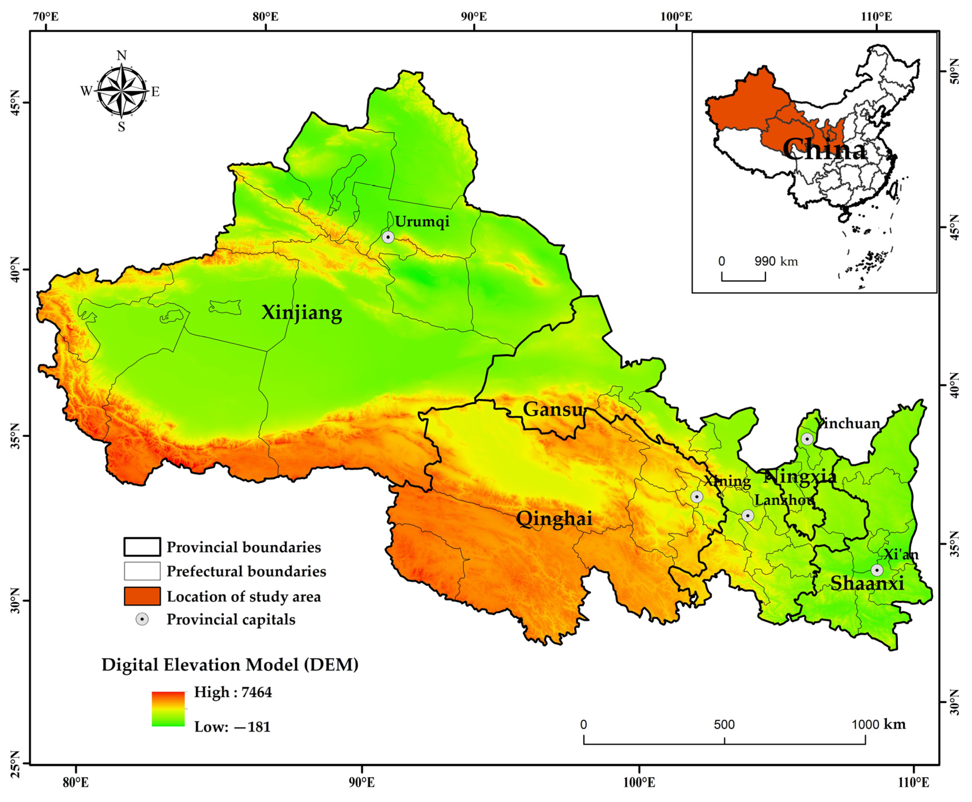
2. Study Area
3. Materials and Methods
3.1. AWUE Evaluation Indicator System
3.2. Exploratory Spatial Data Analysis (ESDA)
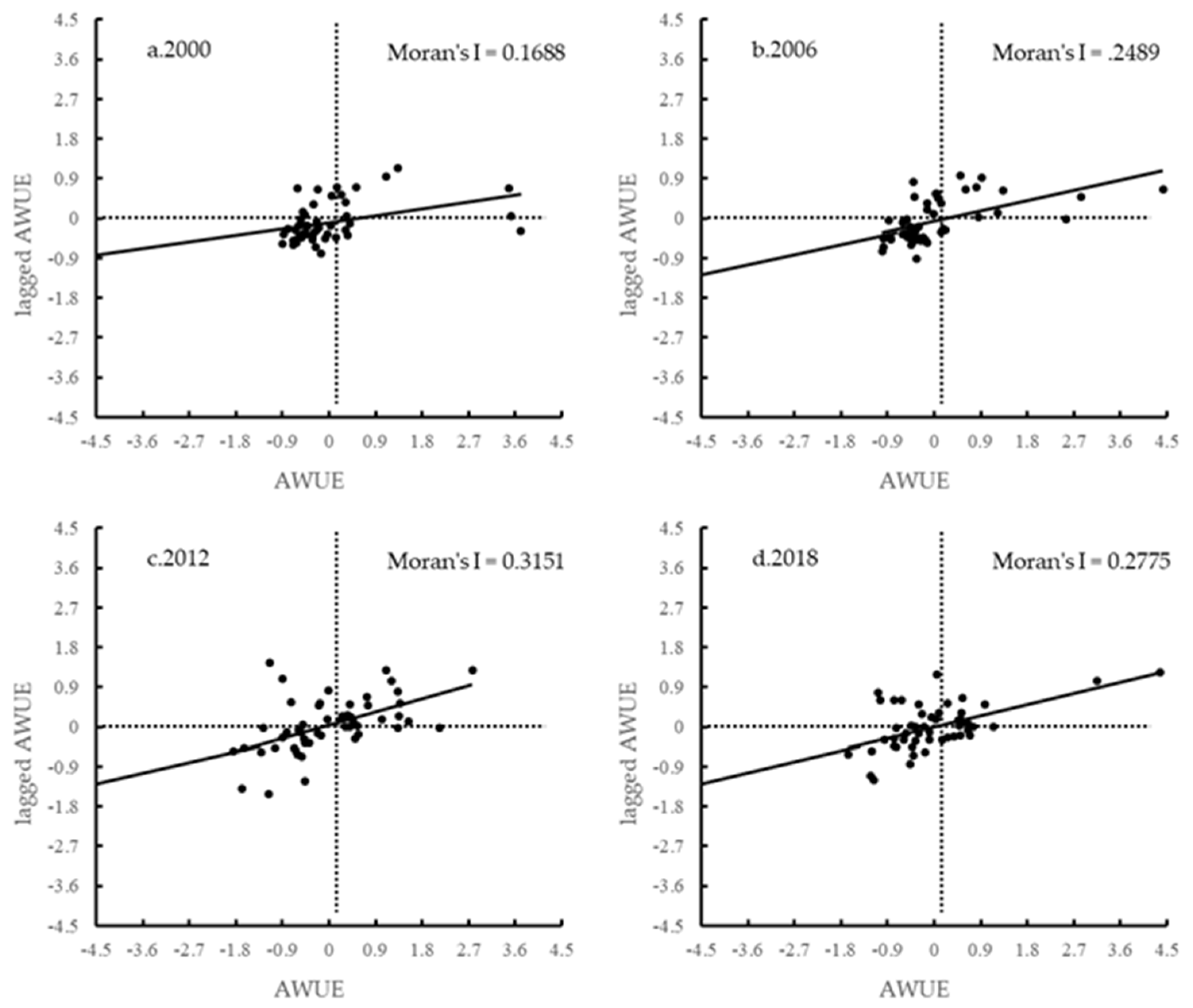
3.2.1. Global Spatial Autocorrelation
3.2.2. Local Spatial Autocorrelation (LISA)
3.3. Spatial Econometric Model
3.3.1. SLM Model
3.3.2. SEM Model
3.4. Variable Selection
3.5. Data Sources
4. Results and Discussion
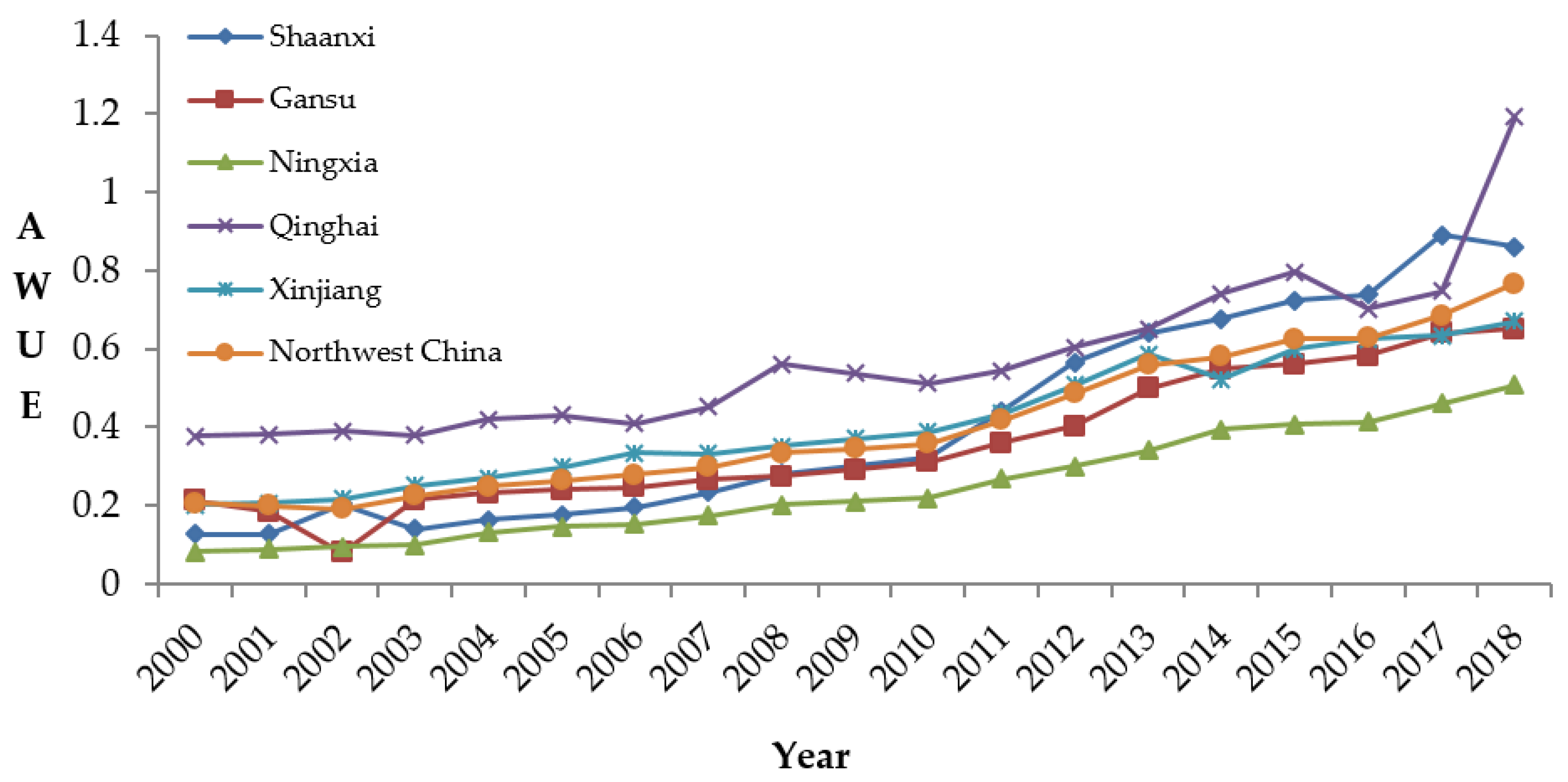
4.1. Calculation of AWUE in Northwest China
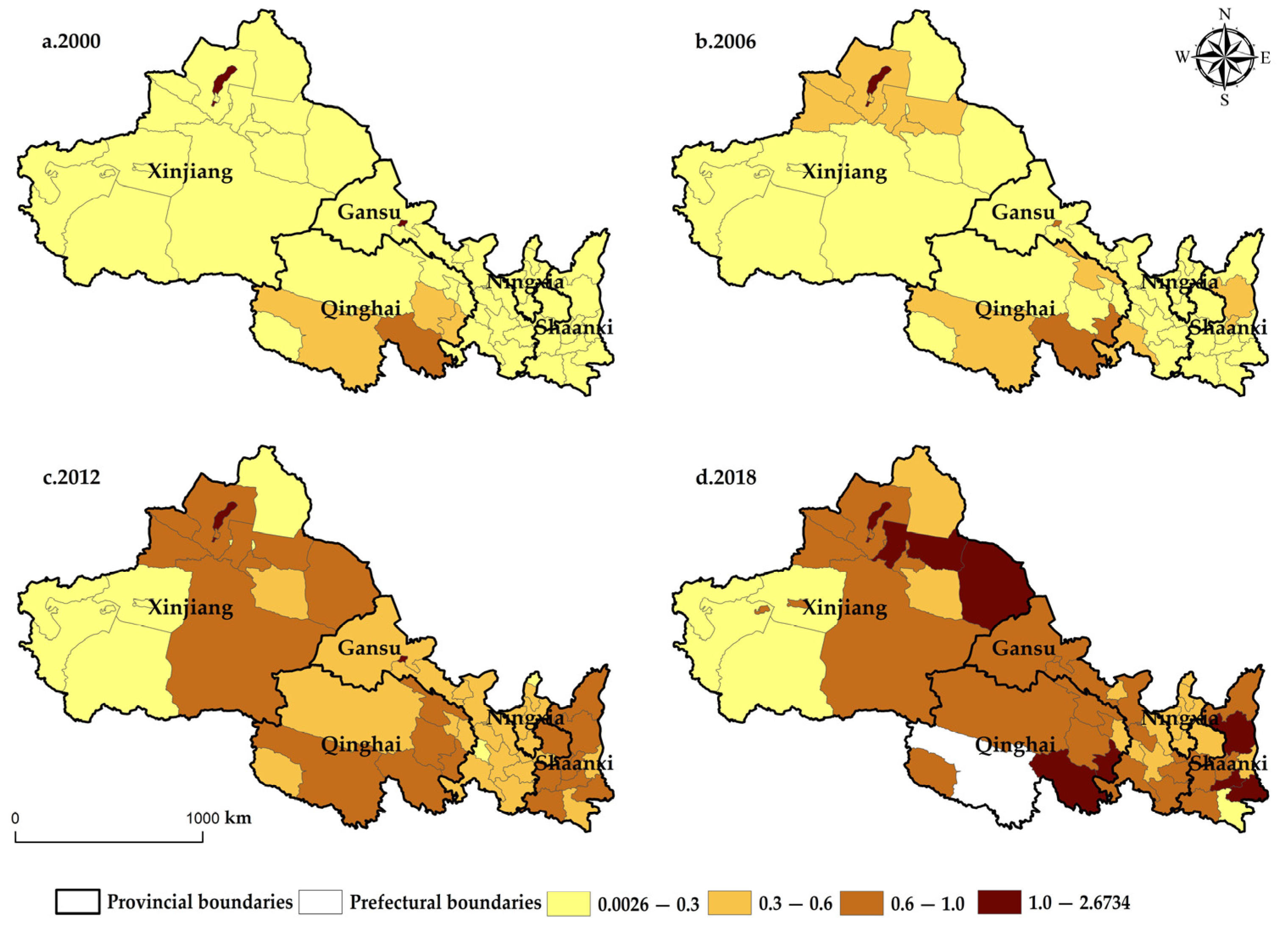
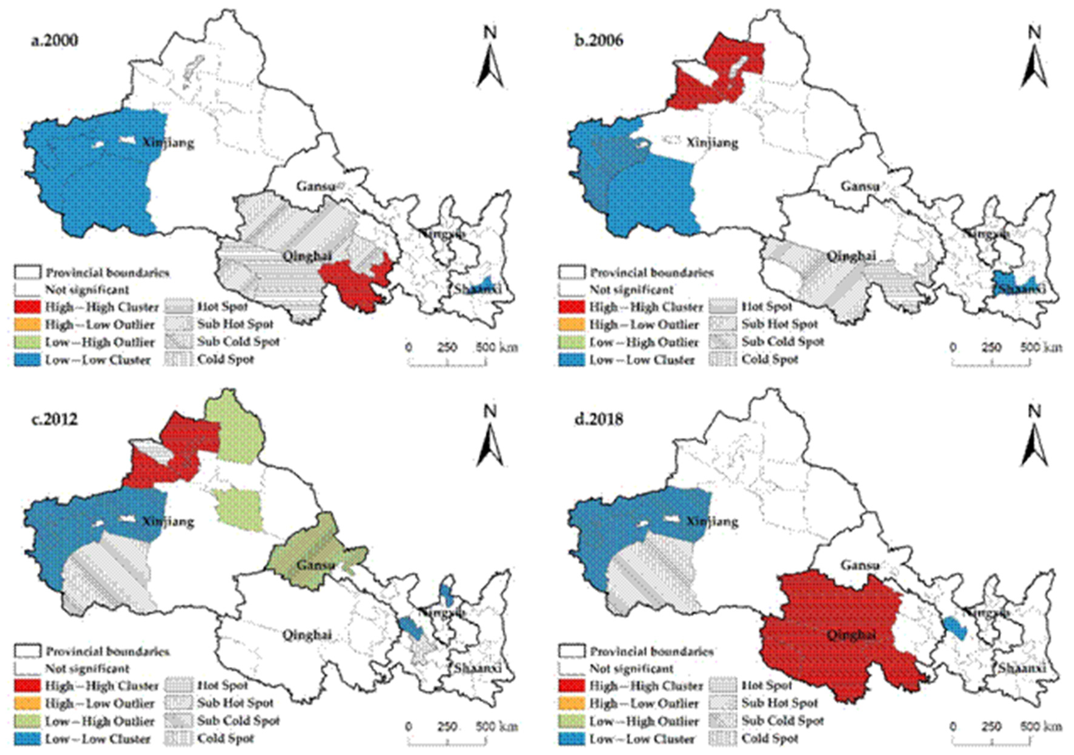
4.2. Spatial Pattern and Differentiation Characteristics of AWUE in Northwest China
4.3. Analysis on the Influencing Factors of AWUE
5. Conclusions
Author Contributions
Funding
Institutional Review Board Statement
Informed Consent Statement
Data Availability Statement
Acknowledgments
Conflicts of Interest
Disclosure Statement
Appendix A

| Regions | 2000 Year | 2001 Year | 2002 Year | 2003 Year | 2004Year | 2005 Year | 2006 Year | 2007Year | 2008 Year | 2009 Year |
|---|---|---|---|---|---|---|---|---|---|---|
| Xi’an | 0.13 | 0.14 | 0.14 | 0.15 | 0.18 | 0.20 | 0.21 | 0.25 | 0.34 | 0.36 |
| Tongchuan | 0.29 | 0.28 | 0.29 | 0.29 | 0.29 | 0.30 | 0.32 | 0.36 | 0.45 | 0.48 |
| Baoji | 0.13 | 0.14 | 0.17 | 0.15 | 0.19 | 0.21 | 0.24 | 0.28 | 0.33 | 0.42 |
| Xianyang | 0.07 | 0.08 | 0.20 | 0.11 | 0.16 | 0.19 | 0.20 | 0.25 | 0.29 | 0.29 |
| Weinan | 0.09 | 0.09 | 0.11 | 0.10 | 0.12 | 0.13 | 0.14 | 0.17 | 0.19 | 0.28 |
| Yan’an | 0.20 | 0.23 | 0.25 | 0.23 | 0.25 | 0.28 | 0.31 | 0.36 | 0.49 | 0.48 |
| Hanzhong | 0.01 | 0.01 | 0.22 | 0.01 | 0.02 | 0.03 | 0.04 | 0.05 | 0.08 | 0.08 |
| Yulin | 0.08 | 0.07 | 0.10 | 0.09 | 0.12 | 0.13 | 0.17 | 0.22 | 0.33 | 0.32 |
| Ankang | 0.09 | 0.10 | 0.23 | 0.16 | 0.10 | 0.06 | 0.07 | 0.09 | 0.11 | 0.20 |
| Shangluo | 0.19 | 0.14 | 0.32 | 0.10 | 0.20 | 0.23 | 0.25 | 0.29 | 0.23 | 0.35 |
| Lanzhou | 0.13 | 0.14 | 0.04 | 0.15 | 0.17 | 0.18 | 0.18 | 0.22 | 0.26 | 0.26 |
| Jiayuguan | 1.05 | 0.91 | 0.35 | 1.04 | 1.01 | 0.95 | 0.90 | 0.87 | 0.72 | 1.01 |
| Jinchang | 0.16 | 0.15 | 0.07 | 0.15 | 0.15 | 0.16 | 0.18 | 0.21 | 0.24 | 0.24 |
| Baiyin | 0.10 | 0.10 | 0.05 | 0.10 | 0.13 | 0.14 | 0.15 | 0.18 | 0.19 | 0.23 |
| Tianshui | 0.11 | 0.12 | 0.04 | 0.12 | 0.13 | 0.14 | 0.13 | 0.05 | 0.11 | 0.11 |
| Wuwei | 0.11 | 0.11 | 0.05 | 0.13 | 0.16 | 0.18 | 0.19 | 0.22 | 0.21 | 0.26 |
| Zhangye | 0.22 | 0.09 | 0.07 | 0.19 | 0.28 | 0.23 | 0.25 | 0.28 | 0.33 | 0.36 |
| Pingliang | 0.24 | 0.10 | 0.06 | 0.17 | 0.27 | 0.21 | 0.23 | 0.27 | 0.29 | 0.26 |
| Jiuquan | 0.07 | 0.04 | 0.08 | 0.20 | 0.08 | 0.26 | 0.30 | 0.32 | 0.37 | 0.38 |
| Qingyang | 0.10 | 0.11 | 0.05 | 0.14 | 0.13 | 0.17 | 0.18 | 0.20 | 0.24 | 0.27 |
| Dingxi | 0.16 | 0.20 | 0.05 | 0.14 | 0.17 | 0.15 | 0.15 | 0.19 | 0.22 | 0.21 |
| Longnan | 0.14 | 0.13 | 0.03 | 0.11 | 0.15 | 0.14 | 0.15 | 0.18 | 0.22 | 0.21 |
| Linxia | 0.11 | 0.12 | 0.06 | 0.12 | 0.13 | 0.14 | 0.15 | 0.17 | 0.17 | 0.16 |
| Gannan | 0.26 | 0.26 | 0.10 | 0.27 | 0.28 | 0.29 | 0.31 | 0.33 | 0.36 | 0.38 |
| Yinchuan | 0.15 | 0.15 | 0.12 | 0.12 | 0.14 | 0.16 | 0.17 | 0.20 | 0.22 | 0.24 |
| Shizuishan | 0.06 | 0.06 | 0.10 | 0.11 | 0.07 | 0.07 | 0.07 | 0.07 | 0.07 | 0.05 |
| Wuzhong | 0.06 | 0.07 | 0.08 | 0.09 | 0.18 | 0.19 | 0.20 | 0.21 | 0.22 | 0.25 |
| Guyuan | 0.09 | 0.09 | 0.10 | 0.10 | 0.13 | 0.15 | 0.16 | 0.21 | 0.22 | 0.29 |
| Zhongwei | 0.06 | 0.06 | 0.06 | 0.06 | 0.13 | 0.17 | 0.17 | 0.19 | 0.23 | 0.26 |
| Xining | 0.09 | 0.09 | 0.10 | 0.10 | 0.10 | 0.12 | 0.13 | 0.17 | 0.21 | 0.23 |
| Haidong | 0.10 | 0.10 | 0.10 | 0.11 | 0.12 | 0.14 | 0.15 | 0.20 | 0.24 | 0.24 |
| Haibei | 0.30 | 0.30 | 0.31 | 0.32 | 0.32 | 0.34 | 0.33 | 0.31 | 0.45 | 0.50 |
| Huangnan | 0.46 | 0.46 | 0.45 | 0.46 | 0.50 | 0.60 | 0.60 | 0.58 | 0.71 | 0.74 |
| Hainan | 0.32 | 0.32 | 0.34 | 0.24 | 0.40 | 0.28 | 0.29 | 0.34 | 0.42 | 0.41 |
| Golog | 1.00 | 1.00 | 1.00 | 0.99 | 0.98 | 1.05 | 0.98 | 0.99 | 1.05 | 0.91 |
| Yushu | 0.51 | 0.51 | 0.55 | 0.55 | 0.66 | 0.62 | 0.50 | 0.73 | 1.11 | 0.76 |
| Haixi | 0.24 | 0.25 | 0.27 | 0.28 | 0.28 | 0.29 | 0.28 | 0.30 | 0.30 | 0.30 |
| Urumqi | 0.21 | 0.23 | 0.31 | 0.49 | 0.61 | 0.62 | 0.58 | 0.54 | 0.52 | 0.51 |
| Kelamayi | 1.01 | 1.00 | 1.00 | 1.00 | 1.00 | 0.99 | 1.36 | 0.91 | 0.98 | 1.03 |
| Shihezi | 0.03 | 0.02 | 0.03 | 0.03 | 0.03 | 0.06 | 0.06 | 0.07 | 0.11 | 0.11 |
| Tulufan | 0.08 | 0.08 | 0.10 | 0.11 | 0.13 | 0.15 | 0.18 | 0.19 | 0.19 | 0.17 |
| Hami | 0.15 | 0.15 | 0.12 | 0.17 | 0.18 | 0.23 | 0.28 | 0.41 | 0.42 | 0.48 |
| Changji | 0.28 | 0.28 | 0.30 | 0.34 | 0.38 | 0.46 | 0.49 | 0.51 | 0.55 | 0.67 |
| Ili | 0.16 | 0.16 | 0.18 | 0.26 | 0.30 | 0.37 | 0.40 | 0.48 | 0.49 | 0.58 |
| Tarbagatay | 0.28 | 0.30 | 0.33 | 0.37 | 0.37 | 0.43 | 0.48 | 0.52 | 0.53 | 0.67 |
| Altay | 0.14 | 0.14 | 0.15 | 0.15 | 0.16 | 0.17 | 0.18 | 0.17 | 0.19 | 0.21 |
| Bortala | 0.28 | 0.29 | 0.30 | 0.36 | 0.39 | 0.41 | 0.43 | 0.46 | 0.45 | 0.53 |
| Bayingol | 0.15 | 0.16 | 0.17 | 0.20 | 0.22 | 0.25 | 0.25 | 0.35 | 0.39 | 0.43 |
| Aksu | 0.05 | 0.05 | 0.05 | 0.05 | 0.06 | 0.07 | 0.07 | 0.09 | 0.11 | 0.13 |
| Kizilsu | 0.17 | 0.17 | 0.18 | 0.18 | 0.18 | 0.20 | 0.20 | 0.21 | 0.20 | 0.20 |
| Kashgar | 0.00 | 0.00 | 0.00 | 0.00 | 0.01 | 0.02 | 0.03 | 0.02 | 0.04 | 0.05 |
| Hoton | 0.05 | 0.05 | 0.05 | 0.05 | 0.04 | 0.04 | 0.04 | 0.03 | 0.03 | 0.04 |
| Regions | 2010 Year | 2011 Year | 2012 Year | 2013 Year | 2014 Year | 2015 Year | 2016 Year | 2017 Year | 2018 Year |
|---|---|---|---|---|---|---|---|---|---|
| Xi’an | 0.45 | 0.48 | 0.60 | 0.69 | 0.73 | 0.76 | 0.81 | 0.87 | 1.27 |
| Tongchuan | 0.49 | 0.55 | 0.64 | 0.68 | 0.72 | 0.76 | 0.75 | 0.76 | 0.78 |
| Baoji | 0.47 | 0.48 | 0.60 | 0.65 | 0.72 | 0.74 | 0.77 | 0.79 | 0.81 |
| Xianyang | 0.45 | 0.54 | 0.61 | 0.66 | 0.76 | 0.84 | 0.87 | 1.89 | 0.98 |
| Weinan | 0.28 | 0.26 | 0.34 | 0.35 | 0.40 | 0.43 | 0.46 | 0.48 | 0.50 |
| Yan’an | 0.54 | 0.62 | 0.76 | 0.84 | 0.89 | 1.01 | 0.95 | 1.01 | 1.06 |
| Hanzhong | 0.15 | 0.40 | 0.49 | 0.67 | 0.85 | 0.79 | 0.88 | 0.96 | 0.98 |
| Yulin | 0.38 | 0.44 | 0.54 | 0.63 | 0.70 | 0.77 | 0.77 | 0.89 | 0.88 |
| Ankang | 0.25 | 0.41 | 0.45 | 0.50 | 0.26 | 0.27 | 0.28 | 0.30 | 0.29 |
| Shangluo | 0.43 | 0.49 | 0.62 | 0.72 | 0.74 | 0.85 | 0.84 | 0.95 | 1.07 |
| Lanzhou | 0.29 | 0.30 | 0.35 | 0.41 | 0.44 | 0.51 | 0.55 | 0.66 | 0.69 |
| Jiayuguan | 0.86 | 1.02 | 0.99 | 1.16 | 1.02 | 0.96 | 1.00 | 1.03 | 0.93 |
| Jinchang | 0.25 | 0.27 | 0.29 | 0.31 | 0.35 | 0.39 | 0.41 | 0.52 | 0.53 |
| Baiyin | 0.28 | 0.27 | 0.31 | 0.37 | 0.42 | 0.44 | 0.46 | 0.49 | 0.51 |
| Tianshui | 0.23 | 0.27 | 0.30 | 0.42 | 0.47 | 0.45 | 0.60 | 0.59 | 0.63 |
| Wuwei | 0.28 | 0.30 | 0.38 | 0.43 | 0.49 | 0.52 | 0.55 | 0.69 | 0.73 |
| Zhangye | 0.38 | 0.42 | 0.47 | 0.55 | 0.62 | 0.61 | 0.61 | 0.68 | 0.68 |
| Pingliang | 0.35 | 0.36 | 0.44 | 0.50 | 0.60 | 0.63 | 0.72 | 0.81 | 0.84 |
| Jiuquan | 0.40 | 0.43 | 0.47 | 0.55 | 0.59 | 0.64 | 0.63 | 0.61 | 0.66 |
| Qingyang | 0.33 | 0.33 | 0.44 | 0.71 | 0.83 | 0.76 | 0.56 | 0.56 | 0.58 |
| Dingxi | 0.26 | 0.25 | 0.30 | 0.38 | 0.44 | 0.41 | 0.42 | 0.43 | 0.43 |
| Longnan | 0.26 | 0.24 | 0.32 | 0.41 | 0.49 | 0.58 | 0.66 | 0.71 | 0.73 |
| Linxia | 0.20 | 0.19 | 0.21 | 0.27 | 0.29 | 0.31 | 0.33 | 0.41 | 0.43 |
| Gannan | 0.46 | 0.40 | 0.46 | 0.52 | 0.63 | 0.63 | 0.67 | 0.74 | 0.74 |
| Yinchuan | 0.31 | 0.33 | 0.39 | 0.43 | 0.46 | 0.48 | 0.52 | 0.54 | 0.57 |
| Shizuishan | 0.10 | 0.11 | 0.10 | 0.14 | 0.37 | 0.38 | 0.41 | 0.43 | 0.45 |
| Wuzhong | 0.22 | 0.28 | 0.29 | 0.33 | 0.34 | 0.35 | 0.36 | 0.26 | 0.34 |
| Guyuan | 0.32 | 0.36 | 0.39 | 0.45 | 0.53 | 0.49 | 0.47 | 0.54 | 0.58 |
| Zhongwei | 0.26 | 0.28 | 0.34 | 0.39 | 0.26 | 0.33 | 0.31 | 0.54 | 0.59 |
| Xining | 0.30 | 0.31 | 0.35 | 0.42 | 0.49 | 0.49 | 0.52 | 0.57 | 0.61 |
| Haidong | 0.25 | 0.34 | 0.38 | 0.40 | 0.38 | 0.44 | 0.38 | 0.39 | 0.45 |
| Haibei | 0.52 | 0.54 | 0.60 | 0.70 | 0.92 | 0.95 | 0.76 | 0.66 | 0.99 |
| Huangnan | 0.75 | 0.78 | 0.80 | 0.93 | 1.01 | 0.96 | 1.02 | 1.01 | 1.01 |
| Hainan | 0.47 | 0.47 | 0.54 | 0.62 | 0.72 | 0.76 | 0.79 | 0.79 | 0.88 |
| Golog | 0.92 | 0.79 | 0.88 | 0.67 | 0.76 | 1.03 | 0.44 | 0.87 | 2.14 |
| Yushu | 0.89 | 0.81 | 0.87 | 0.94 | 1.02 | 1.02 | 0.94 | 0.94 | 2.67 |
| Haixi | 0.37 | 0.38 | 0.39 | 0.51 | 0.63 | 0.72 | 0.76 | 0.75 | 0.79 |
| Urumqi | 0.59 | 0.59 | 0.67 | 0.76 | 0.75 | 0.84 | 0.89 | 0.89 | 0.99 |
| Kelamayi | 0.97 | 0.87 | 0.97 | 1.34 | 0.46 | 0.87 | 0.99 | 0.98 | 1.20 |
| Shihezi | 0.13 | 0.13 | 0.18 | 0.32 | 0.41 | 0.79 | 0.79 | 0.79 | 0.61 |
| Tulufan | 0.21 | 0.20 | 0.22 | 0.31 | 0.32 | 0.36 | 0.37 | 0.37 | 0.43 |
| Hami | 0.52 | 0.46 | 0.65 | 0.77 | 0.65 | 0.74 | 0.85 | 0.91 | 1.05 |
| Changji | 0.71 | 0.78 | 0.90 | 0.99 | 0.96 | 0.91 | 0.98 | 0.90 | 1.10 |
| Ili | 0.60 | 0.68 | 0.78 | 0.90 | 0.95 | 0.94 | 0.83 | 0.92 | 1.00 |
| Tarbagatay | 0.69 | 0.73 | 0.98 | 0.94 | 0.81 | 0.79 | 0.88 | 0.96 | 0.97 |
| Altay | 0.20 | 0.21 | 0.21 | 0.24 | 0.29 | 0.29 | 0.31 | 0.32 | 0.31 |
| Bortala | 0.62 | 0.82 | 0.82 | 0.87 | 0.87 | 0.84 | 0.89 | 0.93 | 0.64 |
| Bayingol | 0.50 | 0.58 | 0.76 | 0.94 | 0.71 | 0.99 | 0.91 | 0.84 | 1.00 |
| Aksu | 0.13 | 0.15 | 0.14 | 0.19 | 0.20 | 0.22 | 0.22 | 0.21 | 0.24 |
| Kizilsu | 0.21 | 0.20 | 0.22 | 0.23 | 0.26 | 0.22 | 0.24 | 0.24 | 0.25 |
| Kashgar | 0.08 | 0.08 | 0.07 | 0.08 | 0.15 | 0.21 | 0.22 | 0.21 | 0.23 |
| Hoton | 0.03 | 0.04 | 0.04 | 0.04 | 0.02 | 0.01 | 0.01 | 0.01 | 0.04 |
References
- Richey, A.S.; Thomas, B.F.; Lo, M.L.; Famiglietti, J.S.; Swenson, S.; Rodell, M. Uncertainty in global groundwater storage estimates in a total groundwater stress framework. Water Resour. Res. 2015, 51, 5198–5216. [Google Scholar] [CrossRef]
- Voeroesmarty, C.J.; Mcintyre, P.B.; Gessner, M.O.; Dudgeon, D.; Prusevich, A.; Green, P. Global threats to human water security and river biodiversity. Nature 2010, 467, 555–561. [Google Scholar] [CrossRef] [PubMed]
- The United Nations World Water Development Report 2018: Nature-Based Solutions for Water. Available online: https://www.unwater.org/publications/world-water-development-report-2018/ (accessed on 19 March 2018).
- Deng, X.P.; Shan, L.; Zhang, H.; Turner, N.C. Improving agricultural water use efficiency in arid and semiarid areas of China. Agric. Water Manag. 2006, 80, 23–40. [Google Scholar] [CrossRef]
- Geng, Q.; Ren, Q.; Nolan, R.H.; Wu, P.; Yu, Q. Assessing china’s agricultural water use efficiency in a green-blue water perspective: A study based on data envelopment analysis. Ecol. Indic. 2019, 96, 329–335. [Google Scholar] [CrossRef]
- Peng, S. Water resources strategy and agricultural development in china. J. Exp. Bot. 2011, 62, 1709–1713. [Google Scholar] [CrossRef] [Green Version]
- Song, P.; Wang, X.; Wang, C.; Lu, M.; Wang, H. Analysis of agricultural water use efficiency based on analytic hierarchy process and fuzzy comprehensive evaluation in Xinjiang, China. Water 2020, 12, 3266. [Google Scholar] [CrossRef]
- Sun, S.K.; Liu, J.; Wu, P.T.; Wang, Y.B.; Zhao, X.N.; Zhang, X.H. Comprehensive evaluation of water use in agricultural production: A case study in Hetao irrigation district, China. J. Clean Prod. 2011, 112, 4569–4575. [Google Scholar] [CrossRef]
- National Water-Saving Action Plan. Available online: http://www.mwr.gov.cn/xw/slyw/201910/t20191016_1365357.html (accessed on 16 October 2019).
- Chen, Y.; Li, B.; Li, Z.; Li, W. Water resource formation and conversion and water security in arid region of northwest china. J. Geogr. Sci. 2016, 26, 939–952. [Google Scholar] [CrossRef] [Green Version]
- Tan, Q.; Zhang, T.Z. Robust fractional programming approach for improving agricultural water-use efficiency under uncertainty. J. Hydrol. 2018, 564, 1110–1119. [Google Scholar] [CrossRef]
- Halsema, G.E.V.; Vincent, L. Efficiency and productivity terms for water management: A matter of contextual relativism versus general absolutism. Agric. Water Manag. 2012, 108, 9–15. [Google Scholar] [CrossRef]
- Hu, J.L.; Wang, S.C.; Yeh, F.Y. Total-factor water efficiency of regions in China. Resour. Policy 2006, 31, 217–230. [Google Scholar] [CrossRef]
- Cao, X.; Zeng, W.; Wu, M.; Guo, X.; Wang, W. Hybrid analytical framework for regional agricultural water resource utilization and efficiency evaluation. Agric. Water Manag. 2020, 231, 106027. [Google Scholar] [CrossRef]
- Liu, X.; Shi, L.; Qian, H.; Sun, S.; Wu, P.; Zhao, X. New problems of food security in northwest china: A sustainability perspective. Land Degrad. Dev. 2020, 31, 975–989. [Google Scholar] [CrossRef]
- Kaneko, S.; Tanaka, K.; Toyota, T.; Managi, S. Water efficiency of agricultural production in china: Regional comparison from 1999 to 2002. Int. J. Agric. Res. Gov. Ecol. 2004, 3, 231–251. [Google Scholar] [CrossRef]
- Azad, M.A.; Ancev, T.; Hernández-Sancho, F. Efficient water use for sustainable irrigation industry. Water Res. Manag. 2015, 29, 1683–1696. [Google Scholar] [CrossRef]
- Mu, L.; Fang, L.; Wang, H.; Chen, L.; Yang, Y.; Qu, X.J. Exploring northwest china’s agricultural water-saving strategy: Analysis of water use efficiency based on an SE-DEA model conducted in Xi’an, Shaanxi province. Water Sci. Technol. 2016, 74, 1106–1115. [Google Scholar] [CrossRef]
- Liu, Y.; Hu, X.; Zhang, Q.; Zheng, M. Improving agricultural water use efficiency: A quantitative study of zhangye city using the static CGE model with a CES water−land resources account. Sustainability 2017, 9, 308. [Google Scholar] [CrossRef] [Green Version]
- Xu, L.; Huang, Y. Measurement of Irrigation Water Efficiency and Analysis of Influential Factors: An Empirical Study of Mengcheng County in Anhui Province. Res. Sci. 2012, 34, 105–113. [Google Scholar]
- Geng, X.H.; Zhang, X.H.; Song, Y.L. Measurement of Irrigation Water Efficiency and Analysis of Influential Factors: An Empirical Study based on stochastic production frontier and cotton farmers’ data in Xinjiang. J. Nat. Resour. 2014, 29, 934–943. [Google Scholar]
- Yu, Z.Y.; Liang, S.M. Analysis of irrigation water using efficiency in arid and semi-arid areas in Northwest China based on Miami model. J. Arid. Land Res. Environ. 2017, 31, 49–55. [Google Scholar]
- Wang, Y. Urban land and sustainable resource use: Unpacking the countervailing effects of urbanization on water use in china, 1990–2014. Land Use Policy 2020, 9, 104307. [Google Scholar] [CrossRef]
- Zhang, X.D.; Zhu, S. Spatial differences and influencing factors of regional agricultural water use efficiency in Heilongjiang province, China. Water Supply 2019, 19, 545–552. [Google Scholar]
- Wang, G.F.; Chen, J.C.; Wu, F.; Li, Z.H. An integrated analysis of agricultural water-use efficiency: A case study in the Heihe river basin in northwest china. Phys. Chem. Earth Parts A/B/C 2015, 89, 3–9. [Google Scholar] [CrossRef]
- Azad, M.A.; Ancev, T. Measuring environmental efficiency of agricultural wateruse: A Luenberger environmental indicator. J. Environ. Manag. 2014, 145, 314–320. [Google Scholar] [CrossRef]
- Tong, J.P.; Ma, J.F.; Wang, H.M. Agricultural Water Use Efficiency and Technical Progress in China Based on Agricultural Panel Data. Res. Sci. 2014, 36, 1765–1772. [Google Scholar]
- Veettil, P.C.; Speelman, S.; Huylenbroeck, G.V. Estimating the impact of water pricing on water use efficiency in semi-arid cropping system: An application of probabilistically constrained nonparametric efficiency analysis. Water Res. Manag. 2013, 27, 55–73. [Google Scholar] [CrossRef]
- Guo, B.; Kong, W.H.; Jiang, L. Dynamic monitoring of vulnerability and quantitative analysis of driving factors in northwest arid desert ecosystem. J. Nat. Resour. 2018, 33, 412–424. [Google Scholar]
- Deng, M.J. “Three Water Lines” strategy: Its spatial patterns and effects on water resources allocation in Northwest China. Acta Geogr. Sin. 2018, 73, 1189–1203. [Google Scholar]
- Huang, Y.J.; Su, Y.; Li, R.L.; He, H.Q.; Liu, H.Y. Study of the spatio-temporal differentiation of factors influencing carbon emission of the planting industry in arid and vulnerable areas in northwest china. Int. J. Environ. Res. Public Health 2019, 17, 187. [Google Scholar] [CrossRef] [Green Version]
- Wang, G.F.; Lin, N.; Zhou, X.X.; Li, Z.H.; Deng, X.Z. Three-stage data envelopment analysis of agricultural water use efficiency: A case study of the Heihe river basin. Sustainability 2018, 10, 568. [Google Scholar] [CrossRef] [Green Version]
- Ma, J.Z.; Wang, X.S.; Edmunds, W.M. The characteristics of ground-water resources and their changes under the impacts of human activity in the arid northwest china—A case study of the Shiyang river basin. J. Arid Environ. 2005, 61, 277–295. [Google Scholar] [CrossRef]


| Variable | Unit | Variable Definition | |
|---|---|---|---|
| Inputs | Land input | khm2 | Total sown area of crop |
| Labor input | 104 labor | Total number of primary industry employees | |
| Capital input | 104 kW | Total power of agricultural machinery | |
| Water input | 104 m3 | Total agricultural water consumption | |
| Technical input | 104 t | Total application amount of agricultural chemical fertilizer | |
| Outputs | Agricultural output value | Hundred million yuan | Total agricultural output value |
| Variable/Unit | Variable Definition | ||
|---|---|---|---|
| Explained Variable | AWUE | Calculated by Super-DEA | |
| Explanatory variables | water resource conditions | per capita water resources(PCW)/% | Total regional water resources/Total population of each region |
| precipitation (PRE)/mm | The depth at which rainfall accumulates on the horizontal plane without evaporation, infiltration and loss | ||
| agricultural modernization | mechanization degree (MECH)/% | Total power of agricultural machinery in various regions/Total planting area of crops | |
| effective irrigation degree(EIG)/% | Effective irrigation area in each region/Total planting area of crops | ||
| economic growth (pGDP)/yuan RMB | GDP per capita | ||
| Socio-economic development | urbanization (URBAN)/% | Urbanization rate of the resident population | |
| City | 2000 | 2009 | 2018 | Mean | Ranking | City | 2000 | 2009 | 2018 | Mean | Ranking |
|---|---|---|---|---|---|---|---|---|---|---|---|
| Xi’an | 0.13 | 0.36 | 1.27 | 0.46 | 19 | Wuzhong | 0.06 | 0.25 | 0.34 | 0.23 | 43 |
| Tongchuan | 0.29 | 0.48 | 0.78 | 0.50 | 14 | Guyuan | 0.09 | 0.29 | 0.58 | 0.30 | 33 |
| Baoji | 0.13 | 0.41 | 0.81 | 0.44 | 20 | Zhongwei | 0.06 | 0.26 | 0.59 | 0.25 | 42 |
| Xianyang | 0.07 | 0.31 | 0.98 | 0.50 | 15 | Xining | 0.09 | 0.23 | 0.61 | 0.28 | 34 |
| Weinan | 0.09 | 0.22 | 0.50 | 0.26 | 40 | Haidong | 0.10 | 0.24 | 0.45 | 0.26 | 39 |
| Yan’an | 0.20 | 0.48 | 1.06 | 0.57 | 11 | Haibei | 0.30 | 0.50 | 0.99 | 0.53 | 12 |
| Hanzhong | 0.01 | 0.08 | 0.98 | 0.35 | 28 | Huangnan | 0.46 | 0.74 | 1.01 | 0.73 | 5 |
| Yulin | 0.08 | 0.32 | 0.88 | 0.40 | 23 | Hainan | 0.32 | 0.41 | 0.88 | 0.49 | 16 |
| Ankang | 0.09 | 0.20 | 0.29 | 0.22 | 44 | Golog | 1.00 | 0.91 | 2.14 | 0.97 | 2 |
| Shangluo | 0.19 | 0.35 | 1.07 | 0.47 | 18 | Yushu | 0.51 | 0.76 | 2.67 | 0.87 | 4 |
| Lanzhou | 0.13 | 0.26 | 0.69 | 0.31 | 30 | Haixi | 0.24 | 0.30 | 0.79 | 0.43 | 21 |
| Jiayuguan | 1.05 | 1.01 | 0.93 | 0.94 | 3 | Urumqi | 0.21 | 0.51 | 0.99 | 0.61 | 8 |
| Jinchang | 0.16 | 0.24 | 0.53 | 0.26 | 36 | Kelamayi | 1.01 | 1.03 | 1.20 | 1.00 | 1 |
| Baiyin | 0.10 | 0.23 | 0.51 | 0.26 | 38 | Shihezi | 0.03 | 0.11 | 0.61 | 0.25 | 41 |
| Tianshui | 0.11 | 0.25 | 0.63 | 0.26 | 35 | Tulufan | 0.08 | 0.17 | 0.43 | 0.22 | 45 |
| Wuwei | 0.11 | 0.26 | 0.73 | 0.32 | 29 | Hami | 0.15 | 0.48 | 1.05 | 0.48 | 17 |
| Zhangye | 0.22 | 0.36 | 0.68 | 0.39 | 24 | Changji | 0.28 | 0.67 | 1.10 | 0.66 | 6 |
| Pingliang | 0.24 | 0.26 | 0.84 | 0.39 | 25 | Ili | 0.16 | 0.58 | 1.00 | 0.58 | 10 |
| Jiuquan | 0.07 | 0.38 | 0.66 | 0.37 | 26 | Tarbagatay | 0.28 | 0.67 | 0.97 | 0.63 | 7 |
| Qingyang | 0.10 | 0.27 | 0.58 | 0.35 | 27 | Altay | 0.14 | 0.21 | 0.31 | 0.21 | 46 |
| Dingxi | 0.16 | 0.21 | 0.43 | 0.26 | 37 | Bortala | 0.28 | 0.53 | 0.64 | 0.59 | 9 |
| Longnan | 0.14 | 0.21 | 0.73 | 0.31 | 31 | Bayingol | 0.15 | 0.43 | 1.00 | 0.52 | 13 |
| Linxia | 0.11 | 0.16 | 0.43 | 0.21 | 47 | Aksu | 0.05 | 0.13 | 0.24 | 0.13 | 50 |
| Gannan | 0.26 | 0.38 | 0.74 | 0.43 | 22 | Kizilsu | 0.17 | 0.20 | 0.25 | 0.21 | 48 |
| Yinchuan | 0.15 | 0.24 | 0.57 | 0.30 | 32 | Kashgar | 0.00 | 0.05 | 0.23 | 0.08 | 51 |
| Shizuishan | 0.06 | 0.05 | 0.45 | 0.17 | 49 | Hoton | 0.05 | 0.04 | 0.04 | 0.03 | 52 |
| Model Selection | W1 | W2 | ||
|---|---|---|---|---|
| χ2 | P | χ2 | P | |
| LM test no spatial lag | 15.996 | 0.000 | 1.489 | 0.222 |
| Robust LM test no spatial lag | 7.469 | 0.006 | 16.017 | 0.000 |
| LM test no spatial error | 8.528 | 0.003 | 4.633 | 0.031 |
| Robust LM test no spatial error | 0.001 | 0.980 | 19.159 | 0.000 |
| Variables | W1 | W2 | Model 5 | ||
|---|---|---|---|---|---|
| Model 1 | Model 2 | Model 3 | Model 4 | ||
| l.lnAWUE | 0.755 *** (14.28) | 0.751 *** (16.31) | |||
| lnPCW | −0.058 *** (−3.14) | −0.033 *** (−3.16) | −0.058 *** (−2.87) | −0.024 ** (−2.48) | −0.459 *** (−2.63) |
| lnPRE | −0.002 (0.06) | −0.006 (−0.23) | −0.020 (−0.44) | −0.026 (−1.05) | 0.016 (0.36) |
| lnURBAN | 0.223 ** (2.17) | 0.071 * (1.72) | 0.268 *** (3.27) | 0.073 ** (1.98) | 0.129 *** (4.19) |
| lnpGDP | 0.663 *** (6.07) | 0.200 *** (2.87) | 0.565 *** (7.27) | 0.198 *** (2.68) | 0.835 *** (28.13) |
| lnMECH | 0.075 (0.75) | 0.039 (0.73) | 0.092 (1.17) | 0.016 (0.31) | 0.074 ** (1.70) |
| lnEIG | 0.258 ** (2.19) | 0.160 *** (3.18) | 0.254 *** (2.57) | 0.176 *** (3.24) | 0.180 *** (2.61) |
| ρ | 0.163 ** (2.11) | 0.031 (0.74) | 0.129 ** (2.29) | 0.073 * (1.74) | |
| sigma2 | 0.136 *** (4.44) | 0.074 *** (4.67) | 0.162 *** (4.16) | 0.055 *** (6.99) | 0.419 |
| Adj-R2 | 0.687 | 0.828 | 0.655 | 0.854 | 0.649 |
| LogL | −79.701 | −90.369 | −132.883 | 39.9647 | 271.310 |
| N | 936 | 936 | 936 | 936 | 936 |
Publisher’s Note: MDPI stays neutral with regard to jurisdictional claims in published maps and institutional affiliations. |
© 2021 by the authors. Licensee MDPI, Basel, Switzerland. This article is an open access article distributed under the terms and conditions of the Creative Commons Attribution (CC BY) license (http://creativecommons.org/licenses/by/4.0/).
Share and Cite
Lu, W.; Liu, W.; Hou, M.; Deng, Y.; Deng, Y.; Zhou, B.; Zhao, K. Spatial–Temporal Evolution Characteristics and Influencing Factors of Agricultural Water Use Efficiency in Northwest China—Based on a Super-DEA Model and a Spatial Panel Econometric Model. Water 2021, 13, 632. https://doi.org/10.3390/w13050632
Lu W, Liu W, Hou M, Deng Y, Deng Y, Zhou B, Zhao K. Spatial–Temporal Evolution Characteristics and Influencing Factors of Agricultural Water Use Efficiency in Northwest China—Based on a Super-DEA Model and a Spatial Panel Econometric Model. Water. 2021; 13(5):632. https://doi.org/10.3390/w13050632
Chicago/Turabian StyleLu, Weinan, Wenxin Liu, Mengyang Hou, Yuanjie Deng, Yue Deng, Boyang Zhou, and Kai Zhao. 2021. "Spatial–Temporal Evolution Characteristics and Influencing Factors of Agricultural Water Use Efficiency in Northwest China—Based on a Super-DEA Model and a Spatial Panel Econometric Model" Water 13, no. 5: 632. https://doi.org/10.3390/w13050632