1. Introduction
Leakages in water distribution systems are a global issue and are becoming increasingly important for water utilities [
1,
2]. The volumes of losses vary significantly according to the maintenance and management of the systems [
3]. In fact, for most water agencies, keeping the pipe networks in good conditions represents a challenging and difficult task, since many pipelines were installed in the first part of the twentieth century, and today, they are often in poor conditions and continue to deteriorate [
4,
5]. As an example, in the UK and in Italy, the amounts of water lost are, respectively, about 25% and 40% of the system inputs. [
6,
7]. Leaks represent a significant cost for water utilities, given that in most cases, the water has to be treated and pumped into the system. Indeed, economic damage due to water losses worldwide can be conservatively estimated at USD 14 billion per year [
8]. Moreover, breaks and low hydraulic pressure can potentially health and safety issues, as pathogens from contaminated materials surrounding water pipes can be brought into the water supply through leakages [
9,
10]. Nevertheless, while water distribution systems worldwide are aging, deteriorating, and seriously compromising the quality of water reaching the consumer, the population is growing and the demands on these systems are ever increasing [
11]. However, the availability of water resources is declining, as it was estimated that two out of every three people will live in water-stressed areas by the year 2025 [
12]. As water is a precious and limited resource, it must be preserved.
The economic, safety, and environmental damages caused by leakages are clearly an issue, and water loss is acknowledged as one of the main challenges for water distribution systems, as it affects water utilities and their customers.
In the literature, four basic activities were defined for loss management and effective control [
13,
14]. The first is pipeline and asset management, as infrastructure naturally deteriorates with time, causing a tendency of a natural increase in the rate of bursts and leaks. This management involves maintenance of service connections, rehabilitation for corroded mains, and even replacement of water pipes. However, this is considerably expensive for the water utilities; due to the high costs involved, in most situations, the networks are not being renewed at a rate that is likely to produce rapid and significant improvements. The second activity concerns active leakage control, that is, identifying and locating unreported leaks, reducing possible damages to both private and public property, and minimizing the volume lost. The consecutive step is repairing the leaks that are found, and in fact, the third activity concerns the speed and quality of these repairs, as it is not only the flow and volume lost that matter, but also the minimization of the duration of leaks and breaks. The last activity is pressure management. While it is not the answer in every case, it is often one of the most effective measures for reducing leakage [
15]. The reduction of excessive pressure can not only reduce the leakage flow, but also the number of new leaks that occur. The control of surges and rapidly fluctuating pressures brings benefits, such as extension of the life of the water distribution infrastructure.
So, the evaluation of the leakage level, that is, the quantification of the amount of water lost, is a priority for water utilities for assessing the state of the network, choosing the maintenance and replacement to do, and analyzing the results of the implementation of these activities, that is, whether the volume of annual real losses increases, decreases, or remains constant. Additionally necessary is the characterization of the leakage, that is, the analysis of the relationship with pressure. Models that explain how leakages will be affected and evolve as pressure varies are needed to understand whether pressure management can bring benefits. In the literature, both of these aspects have been analyzed with different methods.
In particular, regarding leakage evaluation, various methods have been proposed in the literature. A common approach for water utilities is conducting a water balance. The method consists of evaluating the amount of water lost in the network as the difference between the total input volume and the water consumption in a certain time frame. As it is widely used, the International Water Association (IWA) has produced a standard international water balance structure and terminology [
14,
16]. The accuracy of the evaluation depends on the quality of the available data. In fact, the water utilities usually have at their disposal the time series of the water inflow, but as regards consumption, only the meter readings are collected—generally every four or six months for billing purposes—and this allows for an evaluation of the leakage level only over a very long period. In the absence of consumption data, or to obtain a higher level of confidence in the estimation of water loss volumes, the Minimum Night Flow (MNF) method can be applied [
6,
15] by subtracting from the minimum inflow entering a closed area or district—usually occurring between 2:00 and 4:00—the night-time consumption of the users proposed in the literature.
Regarding the characterization of leakages, different models of the leakage and pressure were analyzed in the literature, such as the power equation and the FAVAD (Fixed and Variable Area Discharge) model [
2,
14,
17].
An overview of the MNF method and the models that characterize the relationship between pressure and leakages is presented in the next section.
2. Background
The MNF method can be used to evaluate the amount of water lost in a District Metered Area (DMA). A DMA is a hydraulic part of the distribution network that is isolated from the rest of the system, and it is normally supplied through a single metered line so that the total inflow to the area can be measured [
18]. In fact, the MNF is the minimum inflow in a DMA, usually occurring between 2:00 and 4:00—a period in which user activities are limited and their consumption is at its minimum—while the leakage flow is a significative percentage of the total inflow. The leakage can be evaluated by subtracting a reasonable value of night-time consumption of the users from this value. Different values for night water use have been suggested in the literature according to the places in which they were assessed and according to the types of users, meaning residential or commercial.
Regarding residential users, typically, about the 6% of the population is active during the night, and this activity is almost totally related to the flushing of toilets, which accounts for about 10 L [
19]. That is why, in the literature, a value of 0.6 L/h per person is suggested, or, considering a property composed of an average of 2.5 persons, a value of 1.7 L/h per property of night consumption is proposed. This last value is used in the UK [
6], while other international estimates of residential night consumption range from 3 L/h in Canada to 5 L/h in Malaysia, as well as to 0.4 and 0.8 L/h per person in Germany and Austria, respectively [
20].
Regarding commercial users, the authors of [
19,
20] suggested a simplified value of 8 L/h for all activities. In the UK, different values were evaluated according to the different types of activities [
6], such as 0.9 L/h for churches, gardens, and banks, 6.2 L /h for shops and offices, 12.6 L/h for hotels and restaurants, and 20.5 for hospitals and public toilets.
The accuracy of the leakage level estimation depends on the accuracy of these values, and it should be considered that they do not take into account irregular night water use, such as irrigation or home leakage.
Regarding the characterization of leakage, as previously mentioned, it is a link between the leakage and pressure in order to characterize the evolution of the leak as pressure varies, and its definition is very important for the purpose of pressure management and leak control. A leak in a pipe through a hole or crack can be considered as flow through an orifice, and a great deal of research on different shapes and types was conducted considering the hydraulics of orifices. The relationship between leakage and pressure is described by Torricelli’s equation, which is derivable from energy balance, defining the leakage flow rate Q (m
3/s) from an orifice as [
21,
22]:
where
A is the area of the orifice (m
2),
g is the gravitational acceleration (m/s
2),
h is the pressure head (m), and
Cq is a flow coefficient ( ).
However, in practice, it has been found that the orifice equation does not provide a satisfactory model for the behavior of leakage and pressure [
23]. To apply this relationship in water distribution systems, a more general equation is used, which is in the form of a power equation:
where
Q is the leakage flow rate,
h is the pressure head,
C is the leakage coefficient (m
3-N1/s), and
N1 is the leakage exponent ( ). This relationship is one of the most commonly used equations, and it has also been adopted by the IWA [
14,
24,
25]. However, making the exponent of the leakage equation a variable severs it from its fluid mechanics foundations and turns it into a purely empirical equation [
26]. While the value of
N1 should be 0.5 to be consistent with the hydraulic of orifices, field tests have shown that the coefficient
N1 can take values even greater than 2 [
2,
24].
Further studies were carried out to study the relationship between pressure and leaks. Finite element modeling, under the hypothesis of linear elastic behavior, was used to analyze the behavior of water pipes with different materials and leak openings under different pressure conditions. It was found that the leak area increased linearly with pressure, independently of the pipe’s dimensions, material, and loading conditions [
27,
28,
29,
30,
31]. This means that the leak area
A can be described as being composed of a fixed area and a variable area according to the pressure:
where
A0 is the initial area at zero head differential (m
2),
m is the head-area slope (m
2/m), and
h is the pressure head.
Substituting Equation (3) into Equation (1), a new relationship between leakage and pressure can be found, which is physically based:
where
Q is the leakage flow rate,
h is the pressure head,
g is the acceleration due to gravity,
Cq is the flow coefficient—usually equal to 0.65—
A0 is the initial area at zero head differential, and
m is the head-area slope. This model was first proposed by May in 1994 [
17] and is commonly called the Fixed and Variable Area Discharge (FAVAD) equation. The first term of Equation (4) is the orifice equation and describes the flow through a fixed initial area of the leak. The second term in the equation describes the flow through the expanded area of the leak [
26].
Experimental studies were conducted with various leak types, such as round holes and longitudinal cracks, and different types of materials, such as steel, asbestos cement, and PVC, with laboratory tests on single pipes [
26,
32]. The results showed that for round holes, the measured value of the leakage exponent
N1 was about 0.5 and the value of the head-area slope
m is almost 0, meaning that round holes can be assumed to adhere to the orifice equation, regardless of the pipe’s material. On the contrary, the head-area slopes of longitudinal slits were found to be the largest of all the leak types tested, especially for PVC, with an analogous behavior for the coefficient
N1, whose value was higher than 1.
In order to apply these equations to a water distribution system, the values of the coefficients must be evaluated. Generally, a DMA is considered and a zonal night test is performed. The minimum night flow, which mainly consists of leakage at night, is measured, along with the average night pressure before and after a reduction of the pressure over a limited range. The following equations are then used to evaluate the coefficients [
33,
34,
35]:
where
Q1 and
h1 are the leakage flow and pressure head before the pressure maneuver, and
Q2 and
h2 are leakage flow and pressure head after the pressure maneuver.
Van Zyl and Cassa [
23,
27] investigated the relationship between the FAVAD and the power equations, trying to find a way to convert the leakage exponent
N1 and the coefficients
m and
A0. First, an analytical exploration is performed by matching the two relationships (Equation (2)) and (Equation (4)):
Then, both sides can be divided by the orifice formula (Equation (1)):
The term on the right was defined as the Leakage Number (
LN), a pure number assessed as the ratio between the variable and fixed leakage area:
Through further manipulation, an expression can be found for
N1:
Furthermore, the limits of the pressure head
h in this equation were explored [
23,
27]. As
h is reduced to zero, the leakage exponent
N1 tends to 0.5 and the coefficient
C tends to
. Thus, at pressures of almost zero, the leak behavior is described by the orifice equation (Equation (1)). However, in the limit as
h increases to infinity, the leakage exponent
N1 tends to 1.5 and
C tends to
. Thus, if the pressure is sufficiently high, the FAVAD model (Equation (4)) describes the leak behavior.
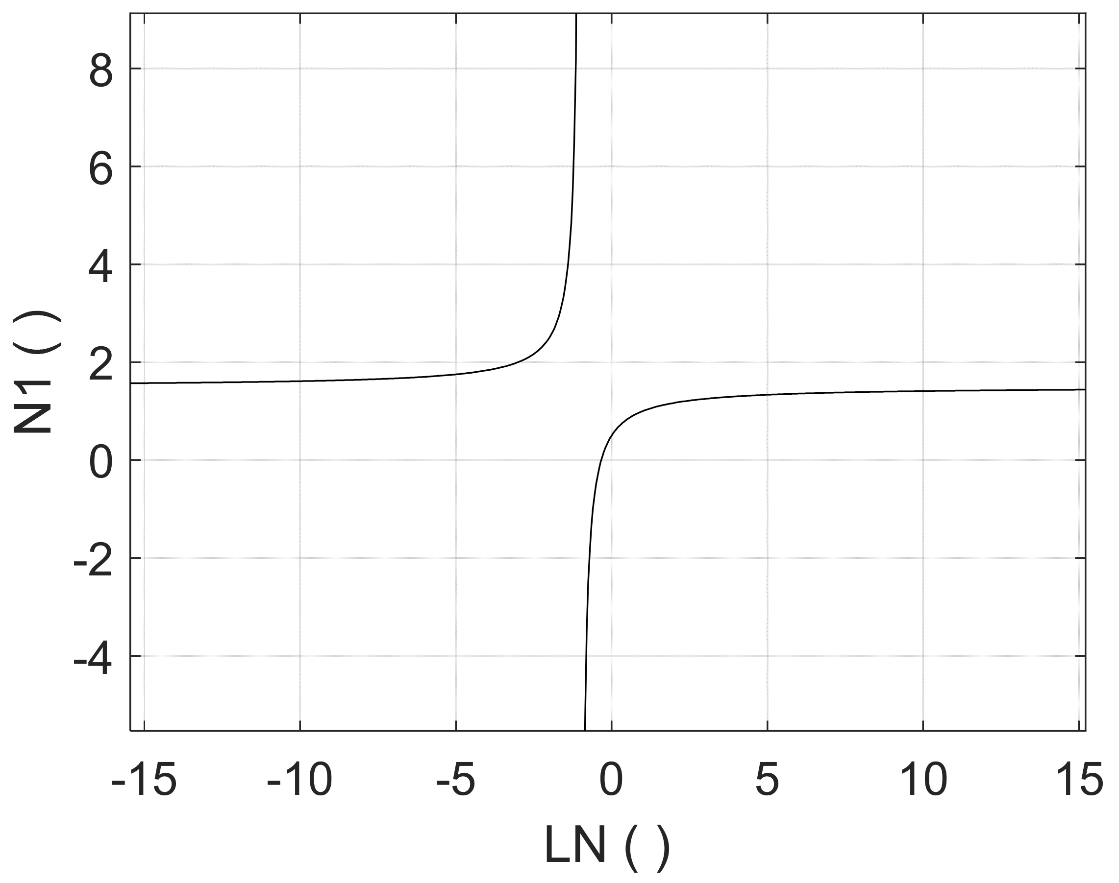
The expression for
N1 (Equation (12)) was simplified, which was also corroborated by experimental testing and finite element analysis, to find a formula for the conversion between
N1 and
LN [
23,
27], which is plotted in
Figure 1:
This paper is a further elaboration of the work by Marzola et al. (2020) [
36], and it shows the results of the application of the water balance and MNF methods for leakage evaluation in a DMA located in Gorino Ferrarese (FE) in Italy, for which the time series of water consumption for every user and the time series of inflow and pressure at the entry of the DMA were collected with specific time scales for a time frame of 45 days. Then, different methods were used to evaluate the coefficients of the power and FAVAD equations for leakage characterization. The accuracy of the results was analyzed, and the pros and cons were highlighted. Lastly, the estimated coefficients were used to verify their consistency with the conversion formula reported in Equation (13) and in
Figure 1.
3. Materials and Methods
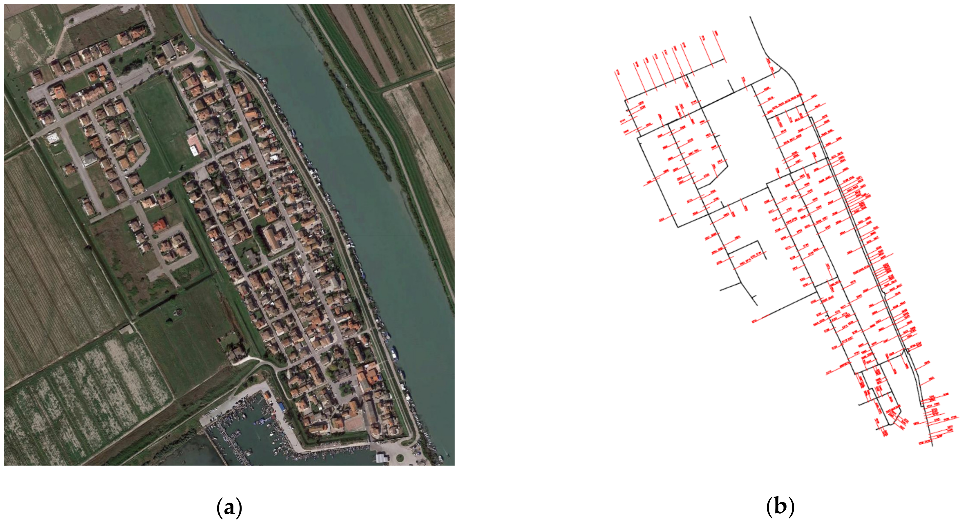
The water distribution system under consideration serves the town of Gorino Ferrarese, a small village located in northern Italy (
Figure 2), which has an area of about 3 km
2. It corresponds to a natural DMA with only one water inflow point, and it supplies 294 users, of which 277 are residential and the remaining 17 represent commercial activities or non-domestic users.
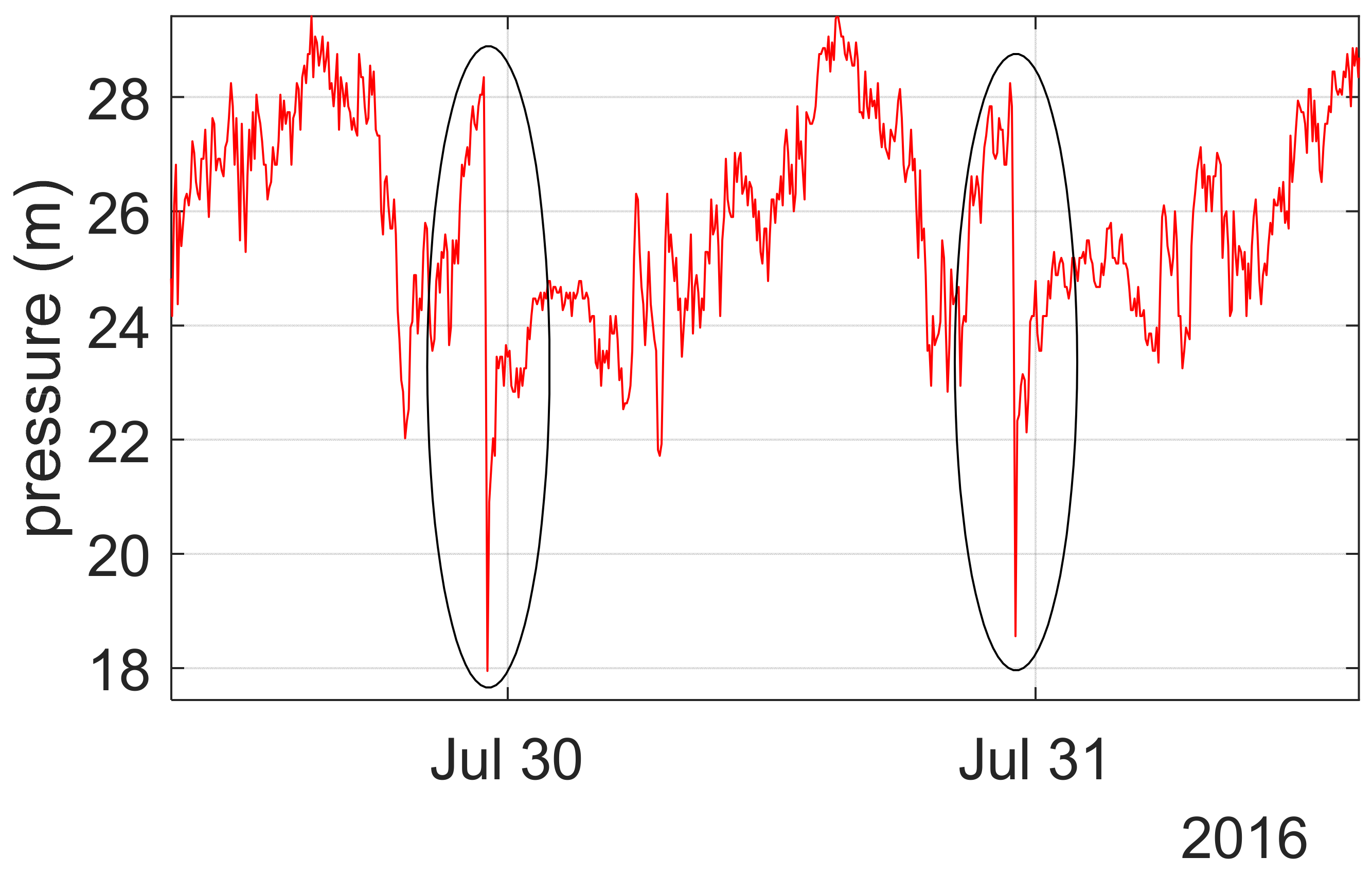
The network pressure is regulated by a pumping station equipped with variable-speed pumps and located nearly 6 km upstream of the DMA. The pumps are controlled in order to keep a pressure of about 30 m immediately downstream from the pumping station itself during the day, while during the night, from 23:00 to 7:00, the pressure control value is reduced of about 10 m, as shown in
Figure 3.
In the spring of 2016, the water utilities managing the network replaced the traditional smart meters with electromagnetic smart meters equipped with data loggers. Operatively, these meter devices could record the value of the cumulative consumed volume with a sensibility of 1 L at time steps that were variable from 1 min to 1 h.
In the summer of 2016 a measurement campaign was performed to collect the time series of (a) the water consumption of each of the 294 users, (b) the DMA inflow, and (c) the pressure at the DMA inlet point from 22 July, 2016 to 4 September, 2016 (45 days) with a 5 min time step.
The time series of the DMA inflow and water consumption of all the users were used to estimate the DMA leakage level by applying the water balance method. Indeed, by subtracting the time series of the DMA’s total consumption, which was obtained by summing up all the users’ consumption time series, from the inflow time series, it was possible to compute the DMA water balance and accurately evaluate the trends in the leakage of the DMA, resulting in a leakage flow of around 0.4 L/s.
Figure 4a shows the DMA inflow (red line) and the sum of all the water used (blue line) for one day as an example, whereas
Figure 4b shows the computed leakage over the entire monitoring period.
The leakage rate resulting from the water balance was thus assumed as a reference value and was used (a) to evaluate the reliability of the MNF method for the quantification of the leakage level and (b) to evaluate the accuracy of different methods for the parametrization of the power and FAVAD equations.
In more detail, with regard to the MNF, the analysis was carried out by extrapolating from the time series of users’ water consumption the minimum flow registered between 2:00 and 4:00 on each monitored day, considering (1) clusters composed of different numbers of residential users (from 5 to 212 users) without home leakages or irregular consumption, (2) all of the previous users with the addition of two users featuring a nightly irrigation of 6 L/min each, and (3) all 294 users of the DMA, including commercial ones. These sets will be indicated hereinafter, respectively, as set 1, set 2, and set 3. The average of the daily values for each set was also computed.
The real values of minimum consumption of these sets were compared with the corresponding ones provided in the literature, which, as previously mentioned, are equal to 1.7 L/h (UK) [
6], 3 L/h (Canada), and 5 L/h (Malaysia) per property, as well as 0.4 and 0.8 L/h per person (in Germany and Austria, respectively) [
20] for residential users, and a general value of 8 L/h [
19,
20] for commercial activities.
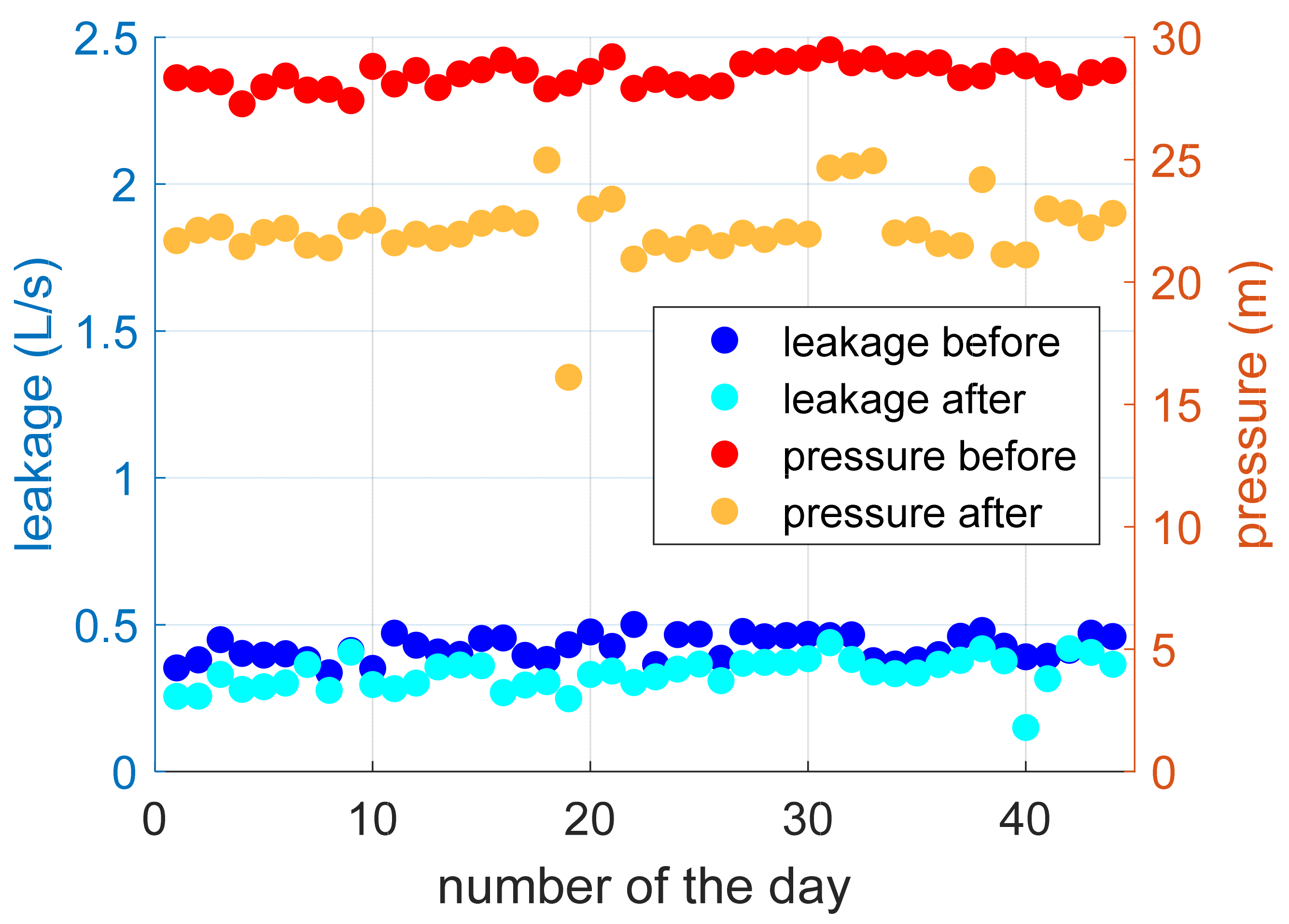
Regarding the relationship between leakage and pressure, the coefficients of the power and FAVAD equations (i.e., exponents
N1 and
C of the power equations (Equation (2)) and the head-area slope
m and fixed area
A0 of the FAVAD equation (Equation (4))) were estimated using different methods. As stated above, these coefficients are, in fact, generally estimated by using a couple of values of pressure and corresponding leakages observed before and after a marked pressure variation. Therefore, the pressure reduction maneuver performed every day at 23:00 was considered, and the pressure and corresponding leakages values observed before and after the reduction were extrapolated from the time series for each of the 45 days monitored, resulting in two pairs of values for each day (
Figure 5).
As a first method, the coefficients were estimated 45 times by using the two pairs of pressure and leakage values observed on a specific day each time. The following equations were used, which were obtained by applying Equations (5)–(8) to these specific data:
where
,
,
, and
are the estimated coefficients of the power and FAVAD equations, respectively, for day
i (from 1 to 45), while
,
,
, and
are, respectively, the leakage flow and pressure head before and after the pressure maneuver of day
i.In the second method, the corresponding values of both flow and pressure before and after the reduction were averaged, and then the two pairs of mean values obtained were used to estimate the coefficients by applying Equations (5)–(8) to these specific data:
where
,
,
, and
are the estimated coefficients of the power and FAVAD equations, respectively, while
,
,
, and
are, respectively, the average values of the leakage flow and pressure head before and after the pressure maneuver.
Thirdly, the method of least squares was applied to all pairs.
For this specific case study, however, thanks to the network monitoring system, the continuous time series of the pressure at the DMA inlet point and the corresponding DMA leakage, which are generally not at the disposal of the water utility, were also available.
Therefore, as the fourth and fifth methods for estimating the coefficients, the method of least squares was applied, considering all the leakages and pressure values observed throughout the 45 days or all the values observed during night-time—from 22:00 until 5:00— in order to be less influenced by daily consumption. All five of these methods, which will be indicated hereinafter as, respectively, MET1, MET2, MET3, MET4, and MET5, were carried out several times to consider data at different time steps, i.e., 5, 10, 15, 30, and 60 min. The coefficients, which were estimated with the corresponding methods and time steps, were compared with each other.
Lastly, regarding the theorical relationship for the conversion between the power and FAVAD equations (Equation (13)), the leakage number (Equation (11)) was evaluated according to the five aforementioned methods. With regard to MET1, the LN was therefore evaluated 45 times by using the estimated values of the coefficient m and A0 (Equations (16) and (17)) for the specific day each time, and, regarding the value of pressure, the average of the two pressure values before and after the maneuver for the same day was considered. For MET2 and MET3, the corresponding coefficients and the averages of all pressure values of the pairs were considered. For MET4 and MET5, the corresponding coefficients and the averages of all the pressure values in the time series or only the averages of the data from 22:00 until 5:00 were considered.
4. Analysis of Results
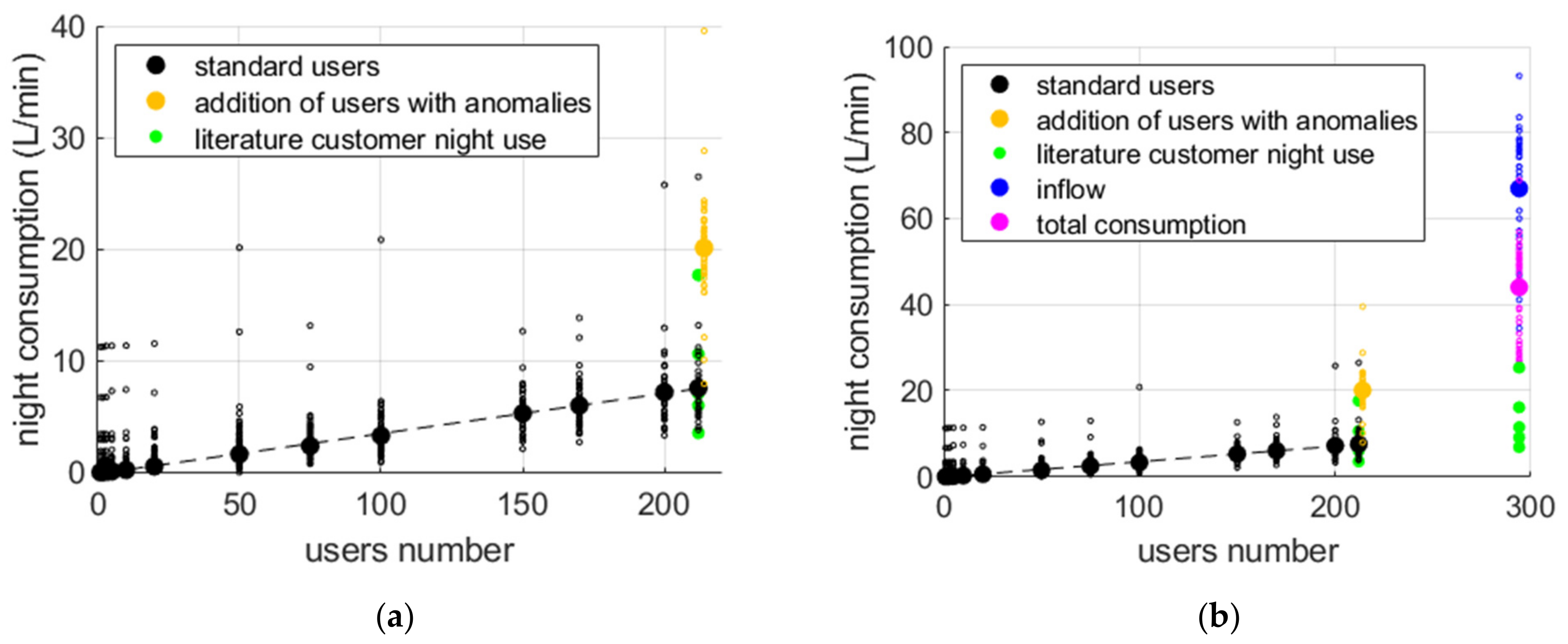
With reference to the results of the application of the MNF method in general and the estimation of the minimum night consumption in particular, in
Figure 6a, the small, empty black dots represent the minimum night consumption for set 1 (i.e., residential users without anomalies, such as leakages within their houses or night irrigation) observed on each monitored day according to the dimensions of the clusters composed of the residential users. In addition, for each cluster, the average value over the 45 days is plotted with a bigger full black dot. As expected, these values increase with a corresponding increase in the number of users, as highlighted by the interpolating straight line evaluated with the least squares method. Regarding the largest cluster (i.e., composed of all the 212 residential users without anomalies), the minimum consumption provided in the scientific literature is plotted with green dots in
Figure 6a, and it can be noticed that almost all of them are a good approximation of both the real minimum night consumption values observed on each day (empty dots) and their mean value (full black dot) for the 212 users. Indeed, a larger value was obtained by considering only the minimum night consumption value provided in the scientific literature for Malaysian users [
20].
However, considering set 2, that is, by additionally including two users with night irrigation, the minimum consumption, which is plotted in yellow in
Figure 6a, highly increased, and the mean value (full yellow dot) even exceeded the one provided in the literature for Malaysia.
Finally, in
Figure 6b, the values of the minimum consumption of all the users in the DMA (i.e., set 3, all 294 users) for each day are plotted with empty magenta dots, and the corresponding values of the minimum inflow in the network for the same days are plotted with empty dots. Clearly, considering their mean values, which are, respectively, plotted with full magenta or blue dots, their difference represents the DMA leakage, which is, in fact, around 24 L/min (i.e., 0.4 L/s), as estimated with the water balance. However, since the time series of the water consumption of each user are difficult to obtain for the water utilities, it is worth noting that if the MNF is applied by subtracting the users’ night consumption provided in the literature, which is plotted with green dots, from the minimum inflow (full blue dot), the leakage would be estimated as three times the actual one. This significant overestimation is mainly due to some residential users with home leakages and to some non-residential activities whose night consumption is very difficult to estimate, such as a football field with a night-time water use of around 20 L/min, which is probably due to irrigation.
Thus, at least for the case study under consideration, we find that the application of the MNF method with values of users’ consumption from the literature would lead to very inaccurate leakage level estimations if the presence of even a few users with anomalies or non-residential users is disregarded, whereas the estimation of the leakage would be consistent if the users’ consumption would not be affected by anomalies, such as home leakages or night irrigation.
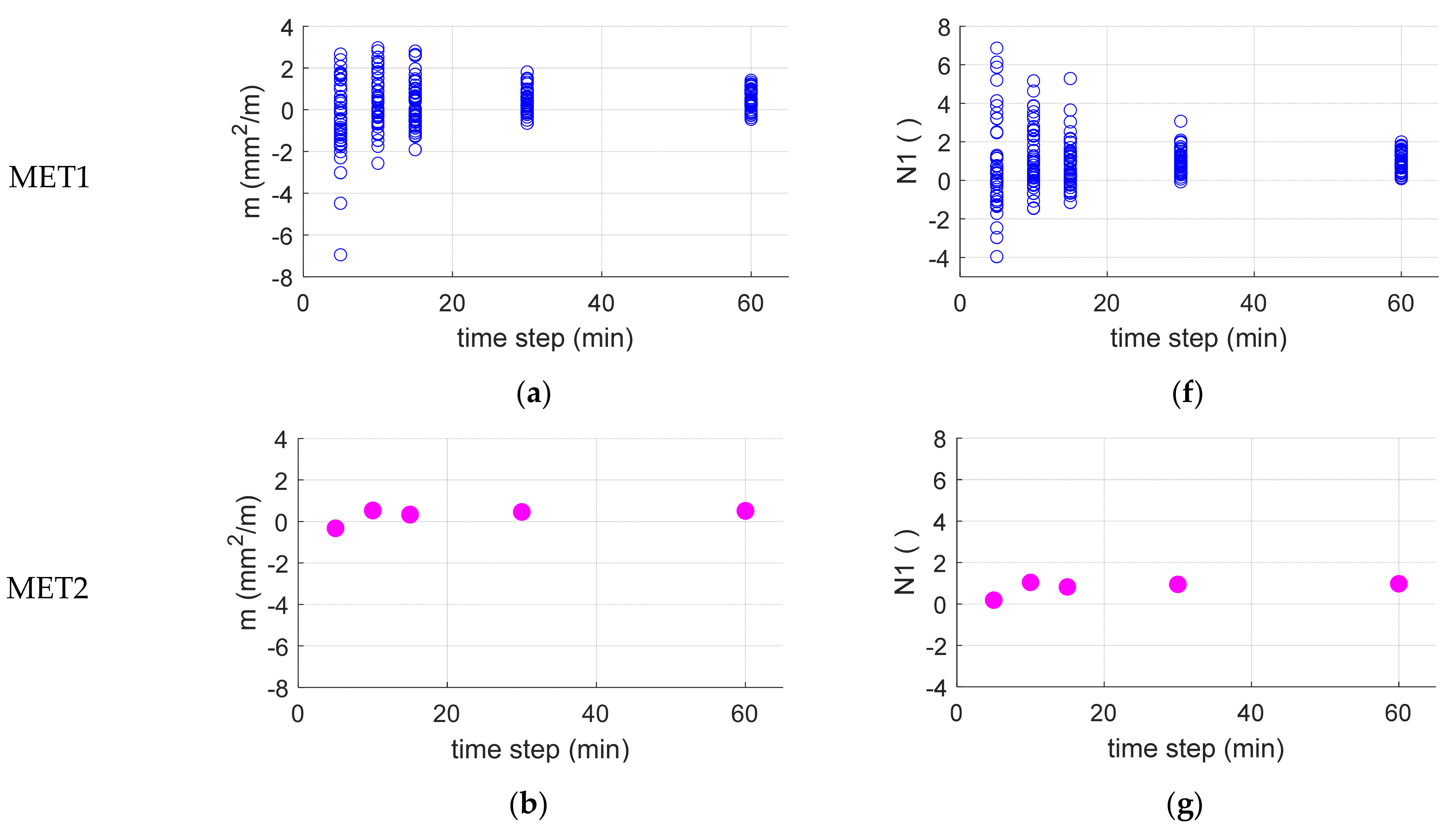
Regarding the characterization of leakages, in
Figure 7, the values of the coefficient
m of the FAVAD equation—representing the head-area slope—and of coefficient
N1 of the power equation—representing the leakage exponent—estimated with the five different methods mentioned above are plotted as a function of the time step characterizing the pressure and leakage time series. By analyzing the results and considering the coefficient
m of the FAVAD equation, it can be noticed that the 45 values resulting from method MET1 (obtained by using the pair of pressures and leakages observed before and after the evening pressure reduction on a specific day from the 45 days monitored) are extremely variable, particularly for quite short time steps, and also present negative numbers that are without physical explanation.
The coefficients estimated with methods MET2 and MET3, i.e., using the averaged pairs and the least squares method with all pairs, still present negative values when short time steps are considered, even if they vary in a smaller range. Therefore, quite inaccurate results can be obtained if only pairs of data acquired by monitoring the pressure and leakage before and after a maneuver are considered. On the contrary, the methods MET4 and MET5, that is, considering a large amount of data observed throughout the entire day or only during night hours, lead to coefficients whose values are independent from the time step considered and more physically sound. Similar considerations also apply for the exponent of the power equation.
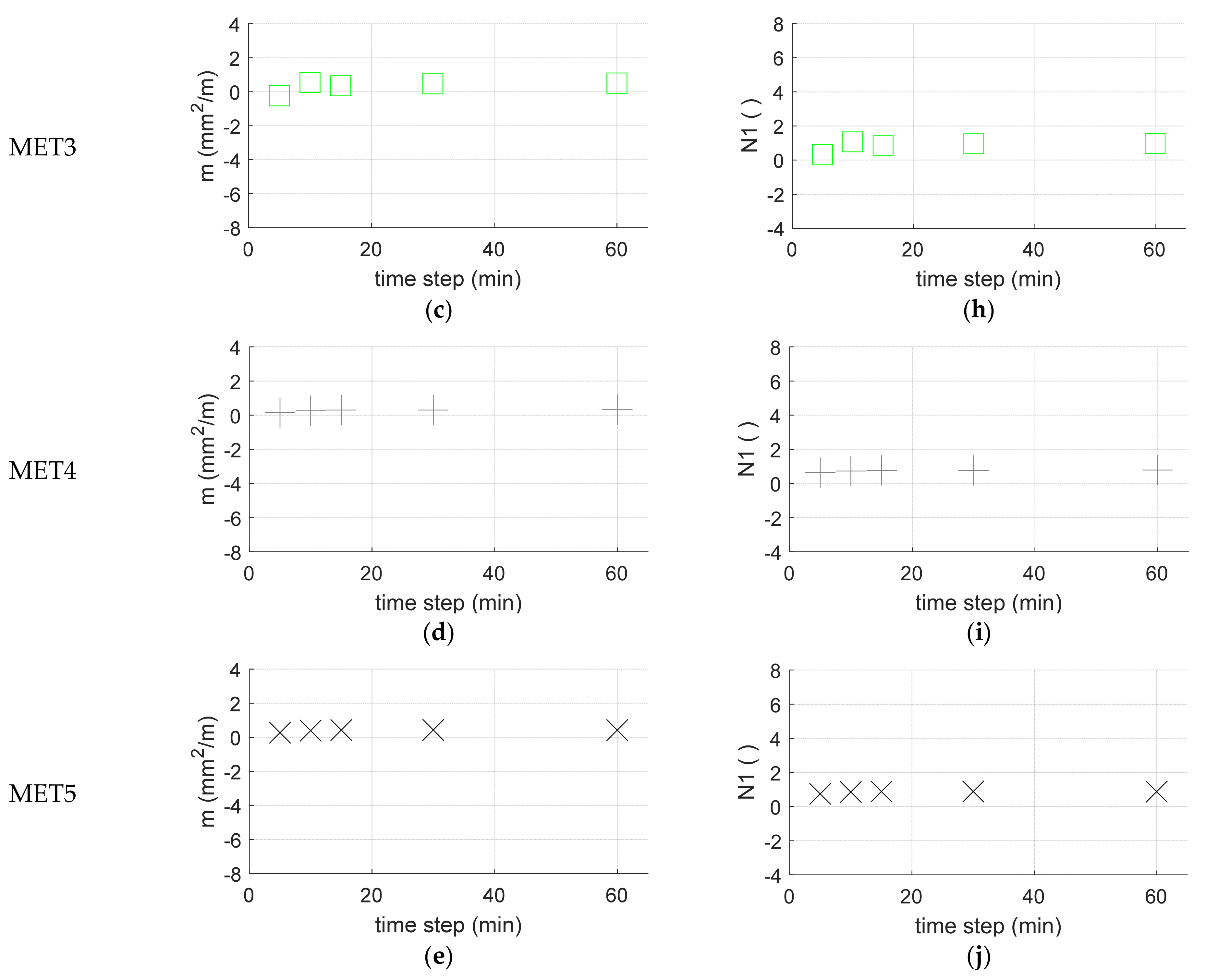
The aforementioned differences between considering one pair (or several pairs) of data observed only before and after a maneuver and the entire time series of pressure and the corresponding leakages are also highlighted in
Figure 8, where the FAVAD equations with coefficients estimated by using the different methods are plotted. As can be observed, the FAVAD equations whose parameters are estimated by using only pairs of data can lead to quite unreliable estimations of the effects of pressure variation on leakage, whereas the FAVAD equations whose parameters are estimated by using the entire time series of pressure and leakages lead to a more consistent estimation.
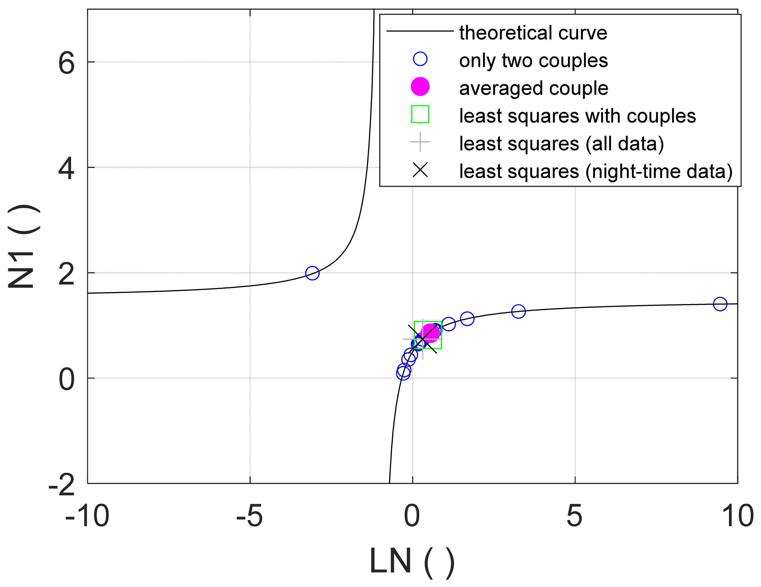
Regarding the conversion formula between the power and FAVAD equations, in
Figure 9, the theoretical equation (Equation (13)) is represented with a black line; the pairs of
N1 coefficients and the corresponding
LN are plotted with different colors and symbols according to the five evaluation methods. As expected, these points fit the theoretical curve because the latter depends only on the relationship between pressure and leakage, that is, the expression of the power and FAVAD equations. These equations were, in fact, always observed independently of the use of different methods of evaluation and different amounts of data.
However, it can be noticed that the points assessed with methods MET2–MET5, that is, by using all of the pairs or the time series, are in a small range and are in a physically valid region, while the 45 pairs of N1 and LN values from method MET1 are scattered all over the theoretical curve up to the limit values, such as negative LN, which correspond to a negative m or A0, which do not have a physical meaning in network systems like the one considered here.
5. Conclusions
In this study, the results of the application of a leakage evaluation in a fully monitored district by using the water balance method and the MNF method with different estimates for the users’ consumption, the differences between various parameterization methods of the power and FAVAD equations for leakage characterization, and the analysis of the formula for conversion between the power and FAVAD equations were presented.
The application of the water balance was performed by subtracting the time series of the water consumption of all users in the district from the DMA inflow time series, which provided an accurate estimation of the leakage level. Considering the application of the MNF method, the real values of minimum consumption were compared with those found in the literature. A significant overestimation of the leakage level can be caused by the presence of just a few users with quite “irregular” night-time water use within the district, such as night irrigation, since these water uses are not taken into account in the values from the literature.
Regarding the parametrization of the FAVAD and power equations, different methods were applied to estimate the coefficients. It was observed that the use of only two pairs of pressure and leakage values obtained from the pressure variations, as is generally done in practice by several water utilities, can lead to extremely variable results. The least squares method applied to the entire time series of pressure and the corresponding leakages is trustworthy, even though it is worth highlighting that this information—in particular, the leakage time series—are difficult to obtain and are generally not available to the water utility.
The theoretical formula linking the two relationships between the power and FAVAD equations was compared with the pairs of coefficients obtained using the different methods. The estimated values fit the curve independently of the parametrization method, even though the method based on single pairs led to a high dispersion and scattered points that corresponded to parameters without physical meanings.


