
Application of LSTM Networks for Water Demand Prediction in Optimal Pump Control
by
 , and
, and
Christian Kühnert
1,* ,
,
Naga Mamatha Gonuguntla
1,
Helene Krieg
2,
Dimitri Nowak
2 and
Jorge A. Thomas
1 1
Fraunhofer Institute of Optronics, System Technologies and Image Exploitation IOSB, Fraunhofer Center for Machine Learning, Fraunhoferstraße 1, 76149 Karlsruhe, Germany
2
Fraunhofer Institute for Industrial Mathematics ITWM, Fraunhofer Center for Machine Learning, Fraunhofer-Platz 1, 67663 Kaiserslautern, Germany
*
Author to whom correspondence should be addressed.
Water 2021, 13(5), 644; https://doi.org/10.3390/w13050644
Submission received: 29 January 2021
/
Accepted: 23 February 2021
/
Published: 28 February 2021
(This article belongs to the Special Issue Machine Learning for Hydro-Systems)
Abstract
:Every morning, water suppliers need to define their pump schedules for the next 24 h for drinking water production. Plans must be designed in such a way that drinking water is always available and the amount of unused drinking water pumped into the network is reduced. Therefore, operators must accurately estimate the next day’s water consumption profile. In real-life applications with standard consumption profiles, some expert system or vector autoregressive models are used. Still, in recent years, significant improvements for time series prediction have been achieved through special deep learning algorithms called long short-term memory (LSTM) networks. This paper investigates the applicability of LSTM models for water demand prediction and optimal pump control and compares LSTMs against other methods currently used by water suppliers. It is shown that LSTMs outperform other methods since they can easily integrate additional information like the day of the week or national holidays. Furthermore, the online- and transfer-learning capabilities of the LSTMs are investigated. It is shown that LSTMs only need a couple of days of training data to achieve reasonable results. As the focus of the paper is on the real-world application of LSTMs, data from two different water distribution plants are used for benchmarking. Finally, it is shown that the LSTMs significantly outperform the system currently in operation.
1. Introduction
Every day, water distribution companies are challenged with the decision of how much drinking water should be produced for consumption during the next day. On the one hand, water supply must be guaranteed 24/7. On the other hand, the energy to pump drinking water into the distribution network should be used efficiently. Therefore, in order for the water suppliers to plan the operation of pumping stations, it is crucial to make reliable predictions of the drinking water consumption during the next day. With this knowledge, they can evaluate different operation plans with respect to energy and cost resulting in significant savings. As of today, German water supply operation is not entirely automated. The staff is primarily responsible for the operation and makes use of process control systems that communicate with the sensors installed throughout the network. Based on the water flow and pressure inside the system, operators can decide to switch water transport pumps on and off.
In the research project H2Opt [1], two different drinking water supply companies have been observed with respect to their operation process. Results show that, oftentimes, the pump operation depends heavily on the amount of water that the operator expects to be needed. As such, expectations are often uncertain, and operation planning is done conservatively so that more water is pumped than necessary. Accurate prediction of consumption allows the operators to consider other operational aspects beyond simply guaranteeing the supply of drinking water under all circumstances and, thus, save energy (and money) for the water company.
For the prediction of daily consumption profiles, traditional approaches like persistence models or auto-regressive moving average (ARMA) models, e.g., in [2,3], show good results. Normally, they are combined with some sort of heuristic, e.g., distinguishing models for different seasons [4] to perform even better. Still, in recent years, a growing popularity of machine learning algorithms, especially in the field of deep learning, have led to new approaches in time series prediction. In particular, Long Short-Term Memory networks (LSTM) show promising results. These recurrent neural networks are mainly used in the field of sequence-to-sequence learning [5]. LSTMs have the advantage that additional information can be directly incorporated into the model. Thus, in the case of water distribution networks, the need to combine rigorous prediction models with heuristics in order to take national holidays, weekends, etc. into account is omitted. A wide range of recent literature investigates the possibility of using deep learning and standard ML methods for water demand forecasting. Examples for short-term demand forecasting can be found in [6,7], which consider the daily demand prediction for a single person. While the work in [8] gives a broader review on machine learning and data analytic techniques for urban water management.
This paper focuses on the application of LSTMs for the prediction of water consumption as a base for reliable operation planning of a water distribution plant. The following questions are examined in detail:
- How does an LSTM behave compared with methods that are already in operational use, in detail persistence and auto-regressive models?
- How does incremental or online learning of LSTM models help to improve the prediction accuracy?
- When no historic data are available, can an LSTM model from a different water distribution network be used instead as a starting point?
To answer these question, the performance of the LSTM models is evaluated regarding two different quality criteria:
- The prediction accuracy for the next day is analyzed, in particular, the predictive performance of different LSTMs.
- The applicability of LSTMs in the process of operation planning is investigated.
Note that the main focus of this work lies on the second quality criteria, as the aim of the paper is not to evaluate the prediction accuracy of the methods themselves, but rather the improvement of the operational planning. If the methods help to increase the water consumption prediction but do not improve the operational planning, the current system can be left in operation.
The paper is structured as follows. In Section 2, an overview of the related work in terms of time series prediction is given and LSTM models are introduced. In Section 3, the decision support methodology is explained and two use cases are illustrated. Section 4 describes how to set-up working LSTM models for the use cases. In Section 4, the prediction performance is discussed followed by the results of optimal pump control based on water demand prediction by means of the considered LSTMs. The paper concludes with Section 7 mentioning more ideas for further research.
2. Review of Methods for Time Series Prediction
One approach to the prediction of water consumption profiles is based on naïve predictor models (e.g., in the simplest case assuming that the profile for tomorrow will be the same as today). Several authors made an attempt to put this approach on an automatic base: An et al. [9], for example, derived a method to automatically generate prediction rules, whereas Arampatzis et al. [10] defined a similarity index for days based on attributes such as the day of the week, weather conditions or special events. Vector Autoregressive Models (VAR), representing well-known methods in time series analysis, are also used to predict hourly water consumption. One variant can be found in [11], for example. Beyond these traditional approaches, machine learning methods entered the field of water demand forecast and numerous studies have made use of artificial networks. Adamowski and Karapataki [12] compare three types of artificial neural networks for the prediction of weekly peak water demand with “classical” multiple linear regression models. A similar study is done by Bougadis et al. [13]. However, machine learning methods are also used for daily demand forecasts as looked at in this work. Candelieri et al. [14] imply a data-driven, fully adaptive self-learning algorithm for water demand forecasting that combines time-series clustering with a support vector machine regression. Herrera et al. [15] compare the performance of several machine learning methods for water demand forecast, comprising among others, artificial neural networks, random forests, and support vector regression. Rodrigues Rangel et al. [16] even train one artificial neural network model for each hour of the day and put their predictions together to set up the daily demand forecast.
Still, in recent years, significant advances in time series prediction have been achieved through Long Short-Term Memory (LSTM) networks. These are a special kind of deep learning model and are currently in the center-point of research. In the following, a short introduction is given to naïve predictors and vector autoregressive model, while LSTMs are explained in further detail as they are in the forefront of this paper.
2.1. Naïve Predictors
Naïve prediction models, also known as persistence models, usually follow some sort of heuristic and have a straightforward approach. In most cases, these models are taken as a baseline when testing against other, more sophisticated methods. Examples where persistence models are used for benchmarking are, e.g., in Perez et al. [17] for solar radiation forecasts, Takeyosi [18] for photovoltaic power generation forecasts, or in Kaushik et al. [19] for healthcare. In this publication, a naïve predictor is used based on a heuristic to achieve some sort of an expert system. In detail, a prediction profile is obtained by computing the hourly-wise mean of the last similar days of the week and is considered as the prediction of the next day. The model exhibits increased performance by taking holidays into account. The approach of the naïve predictor is described in Algorithm 1:
| Algorithm 1: Pseudocode for the naïve water consumption prediction model |
 |
2.2. Vector Autoregressive Models (VARs)
For multivariate time series forecasting, VARs are the most widely used method. Besides the prediction of water profiles, vector autoregressive models have been successfully applied in the estimation of brain function connectivity [20], in aviation [21], or economics [22]. Many other applications are, e.g., given in [23]. The main idea behind a VAR is that each variable at time point t is predicted by all variables at time point . Therefore, VARs assume that a time series follows a stochastic process and that linear dependencies exist between the variables.
More formally, a multivariate time series of dimension d at time point is described by a first-order VAR model as
where is a matrix representing the coefficients of the VAR model and is a sequence of independent normally distributed noise with mean 0 and covariance . In Equation (1), for example, the parameter is the autoregressive effect of on and is the cross-lagged effect from on .
2.3. Long Short-Term Memory Network (LSTM)
For time series prediction, VARs are state-of-the-art. Still, in recent years, the growing popularity of machine learning algorithms, especially in the field of deep learning, has led to new approaches for the prediction of time series. Because of their ability to learn long term patterns in sequential data Long Short-Term Memory Networks, originally introduced by Hochreiter and Schmidhuber in 1997 [24], have been applied to several use cases. Recent examples in which LSTMs achieved comparative or better results that established methods are handwriting recognition [25], speech recognition [26,27], machine translation [5], reliability analysis [28], covid-19 transmission [29], and many more. In the water sector, a recent publication in which LSTMs are used is in [30], the authors of which developed a rainfall–runoff model; in [31], which uses LSTMs to forecast water production in solar stills; the authors of [32] make a short-term water quality variable prediction; and the authors of [33] use LSTMs to detect abnormal working conditions in water supply networks.
As LSTMs are the primary models for demand forecasting in this paper, the following subsections continue with further details. They are a special kind of a Recurrent Neural Network (RNN). The key difference is that traditional RNNs have the shortcoming of a vanishing/exploding gradient during training, which makes them unable to learn long-term dependencies in data. LSTMs aim to solve this problem, which makes them especially interesting for the prediction of water consumption profiles, as there exist long-term dependencies like seasons, different behavior for different days of the week, and national holidays.
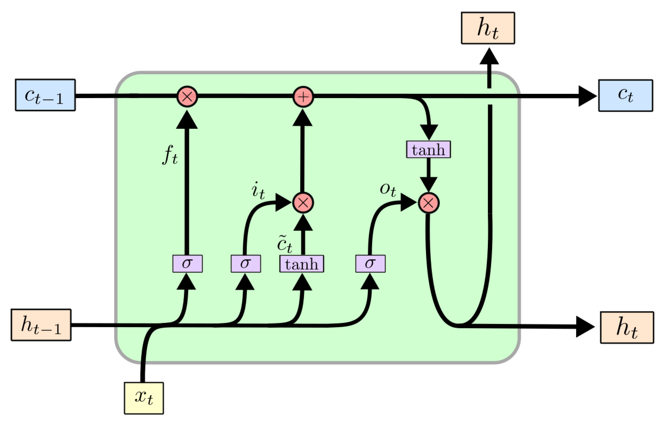
To cope with these types of dependencies, the main concept behind LSTMs is that they consist of cells. A cell of a classic LSTM is shown in Figure 1. In the literature, a LSTM cell is typically separated into three gates, each composed of a layer and pointwise multiplication. Usually, these gates are called the input, output, and forget gates, and are used to regulate the information passing through the cell. Furthermore, a LSTM cell consists of the two cell states and which receive their values from the previous cell. The dimension n describes the number of units (the model order) in the cell. To finalize, defines the input to the cell and the output can be generated through the state . LSTM cells are best explained by passing the three gates one by one. Initially, for the forget gate, the output is generated by
with and . Similar to the forget gate, the input gate is also added to the cell state by calculating and as
with and for and and for . Then, the current cell state is calculated following the operation
with and ⊙ representing the Hadamard product. Finally, the output of the cell is calculated by using the output gate following an approach similar to the forget and input gates:
with , and resulting in and . In the prediction of the water consumption profile, is used as the final output of the LSTM.
2.4. Online Learning with LSTMs
In machine learning, online or incremental learning techniques are used to keep a model up to date with recent data. Like other neural networks, LSTMs have the advantage that their weights can be updated every time step without additional effort and an online learning is easily achieved. Regarding the prediction of water consumption, this comes in handy, as drift effects, occurring e.g., due to the four seasons, can be incorporated into the model. For LSTMs, online learning has been proven to deliver good results, e.g., in speech recognition [35] or land cover prediction [36]. In this paper, the online learning approach for the LSTMs is demonstrated in Section 4, where the weights are updated every time a new consumption profile for the day passed becomes fully available.
2.5. Transfer Learning with LSTMs
In general, transfer learning is used to improve the learning of a new task by transferring knowledge from a similar task to the current one. For LSTMs, as the weights can be easily updated, transfer learning is straightforward. Recent work has been done, e.g., in [37] for named-entity recognition or in [38] for speech recognition. Especially for water consumption, daily profiles from different water utilities share similar behavior resulting in one consumption peak in the morning and another one in the evening. Therefore, it is expected that transferring LSTM knowledge from one network to another will yield good results. This is demonstrated in Section 5.
3. Application: Decision Support for Water Supply Systems
As mentioned in the introduction, in order to efficiently run pumping stations, it is crucial to make reliable predictions of the daily consumption profile for the next day. However, good predictions do not necessarily imply that pumps run efficiently. Therefore, in this paper, the methods are initially compared with respect to their prediction quality of the consumption profile, but the main focus is regarding their ability to improve the overall efficiency of a pumping station. Recent work in the field of the overall optimization of water distribution systems is, e.g., given in [39] or [40], while a good literature review is in [41]. This paper relies on the work that was accomplished in the research project H2Opt [1], where several pilot studies have been conducted to optimize the operation of water supply systems. In the end, a decision support software [42] was developed for a German city of about 100,000 citizens. In further studies, operation was optimized by following the approach of a naïve predictor and assuming that the drinking water consumption of the day under consideration was like the day before.
3.1. Water Suppply System
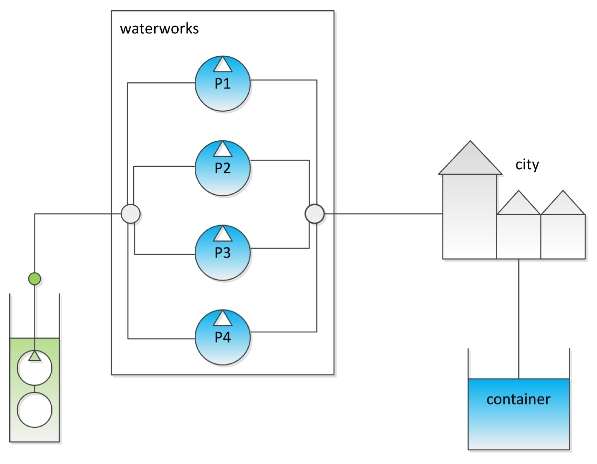
Figure 2 shows the scheme of the water supply system. It consists of the waterworks from which four pumps feed drinking water into the system which is consumed by the city. Superfluous drinking water is stored in a cylindrical container which has a diameter of 42.43 m and a limited filling height of 9 m. It is consumed by the city at times of high demand or when the pumps are turned off. The container allows to delay and possibly improve pump operation. In addition, it is required that 44% of the total container volume must be hold back in case of fire emergency. This means, the container level may not fall below 4 m.
3.2. Decision Support Software
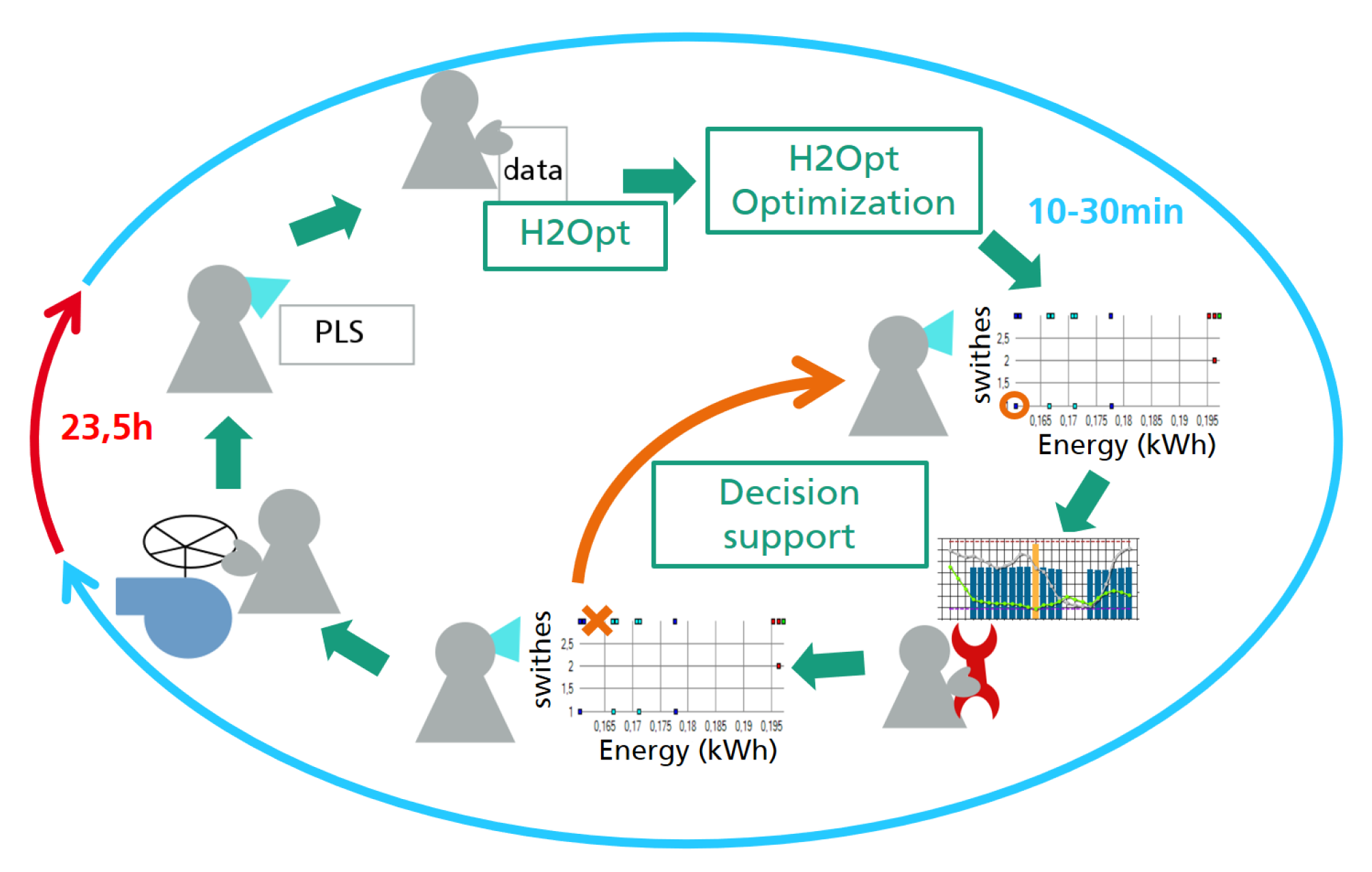
Figure 3 describes the daily interaction with the H2Opt decision support software that the operator at the waterworks goes through in the morning. By means of the software, the operation of the pumps feeding drinking water into the consumption network (see Figure 2) is planned and analyzed. Given the final decision, the operator enters a schedule into the process control logic to control the feed pumps for the next 24 h. This planning horizon is typical for many water supply systems. The schedule is based on hourly time steps. On the one hand, these time steps are fine enough to react to daily water consumption patterns. On the other hand, they prevent pumps to be switched on and off too often. This is important, as sudden pump switches can lead to pressure shocks in the piping system causing wear in both the piping system and the pumps. To match the operation schedule, water consumption shall be predicted on an hourly basis for the next 24 h, as well.
In this paper, the H2Opt software is used for benchmarking the prediction models performing the following steps:
- The evaluated demand forecasting models are used to predict sequences of 24 h consumption profiles for one year. Each profile starts at midnight.
- The resulting profiles are fed into the decision support software and operation plans are computed.
- Beyond the simulation based on the predicted water demand and the computed operation plan, another simulation is performed based on the realized water consumption and the same operation plan.
- The latter simulation must be checked for feasibility. It stays feasible if the water level inside the storage container neither falls below the lower bound given by the firefighting reserve nor exceeds the upper bound, meaning that there is an overflow and water is wasted.
- Finally, both simulations are compared by means of the end-of-day container level of the water tank. The difference measures the prediction quality of the method for each day.
For the water supplier, it is not the complete daily consumption profile, but the end-of-day container level that is the more important value, as the next day’s pump operation is based on this information.
3.3. Use Cases for the Prediction of Water Demand
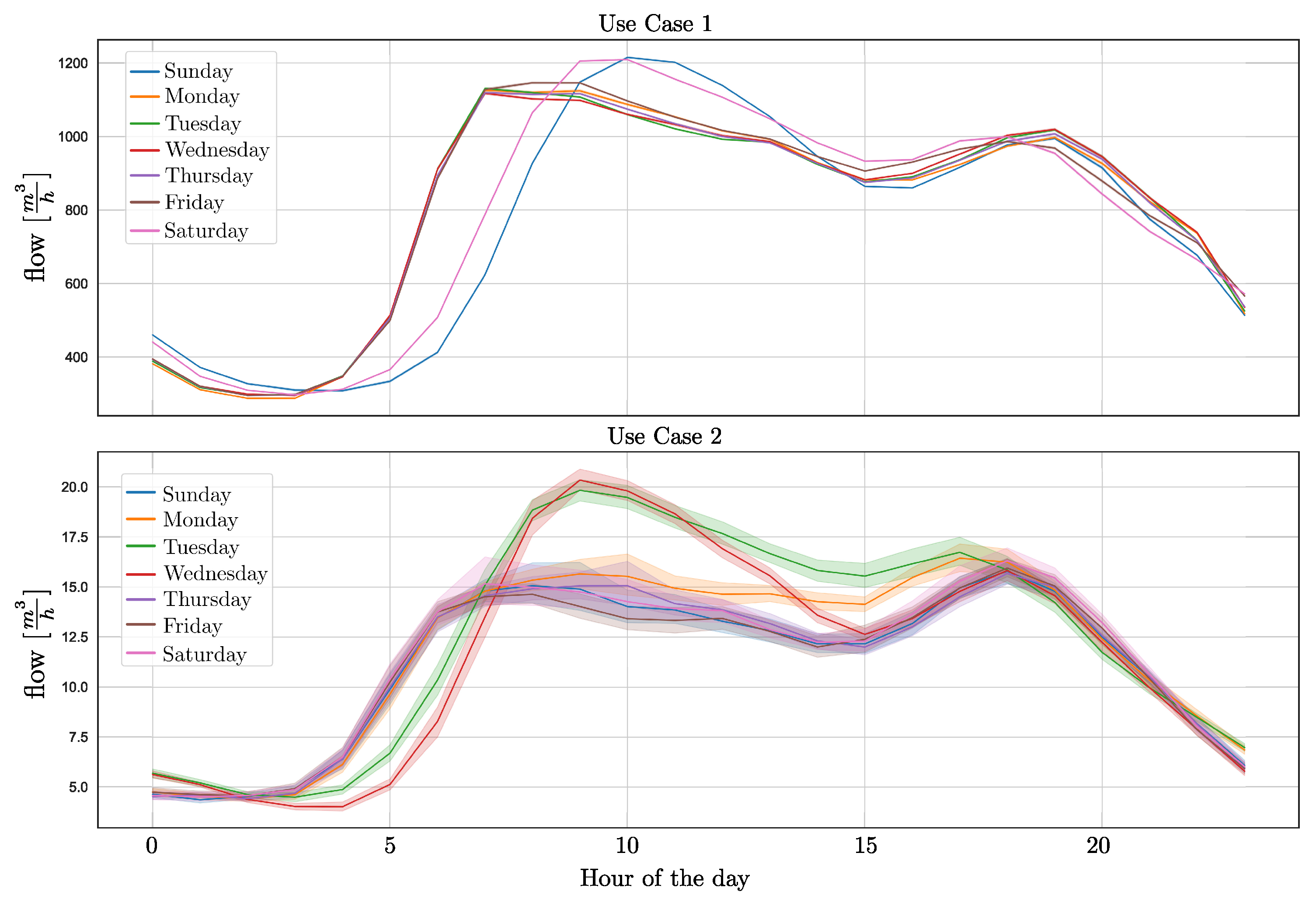
Two use cases are selected for benchmarking the performance of the different methods against each other. Use case 1 is used for a comparison, while use case 2 is used for the LSTM with transfer learning. Table 1 summarizes the data sets of the two use cases, and Figure 4 shows the daily profiles, including the day of week and the standard deviation. As there is only low standard deviation in the data, Figure 4 covers training and evaluation data in one plot for each of the use cases. For exemplary prediction results using the online learning approach, please refer to Figure 8.
In the data sets, the sampling rate was set to 1 h, meaning that the daily profile of the water consumption consists of 24 values. Furthermore, each sample has been enriched with the following meta data: (1) Day of the week: As daily consumption profiles differ especially between working days and weekends, each sample gets as additional information the current day of the week in terms of a number between 0—Monday and 6—Sunday. (2) National holidays: On a national holiday, water consumption follows the behavior of a Sunday. Therefore, each sample is enriched with the information whether it is a normal day, a day before a national holiday or a national holiday.
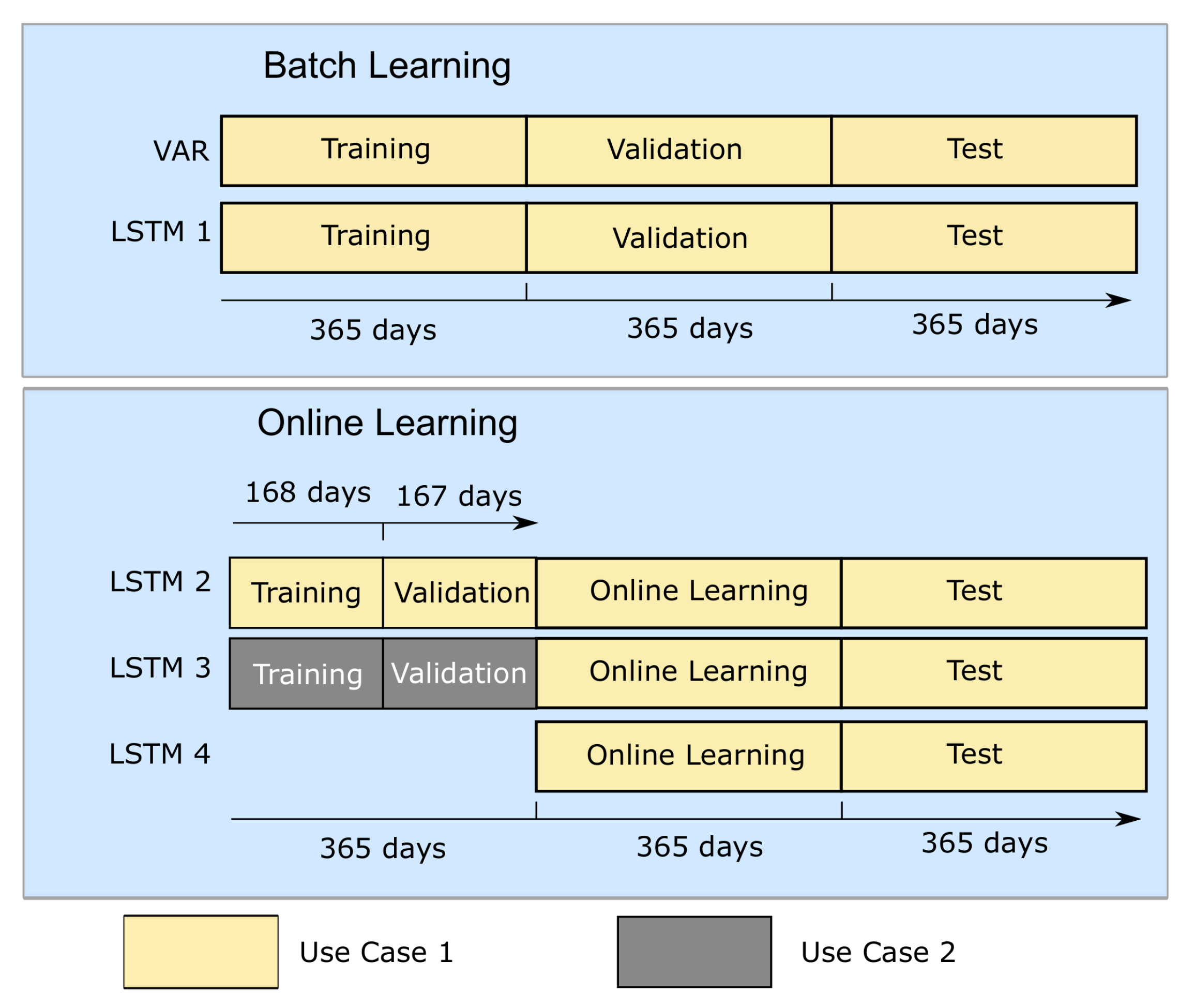
Figure 6 explains the splitting of the data from use case 1 and use case 2 into different sets. For use case 1, data have been split into three equal sets, namely, for training, validation, and testing, while training and validation have been used for model fitting, and the test data set is being used for the actual benchmarking. As use case 2 is used for the evaluation of transfer learning capabilities for LSTMs, the data set only needs to be separated into a training and test set.
4. Experimental Approach
4.1. Model Parameters
For each of the different methods, several parameters need to be set and tuned; these are described in the following.
Naïve predictor: The only parameter the naïve predictor uses as information is the number of the last days of the week in order to calculate an average profile. For the use cases, this means that the predictor always works on the data from last week, therefore the parameter D is set to one.
VAR: As input sequence for the vector autoregressive model, preceding water consumption data, the name of the current weekday and the information whether the day in question is a national holiday or a day before a national holiday are used. The output of the VAR is the daily consumption profile for the next 24 h.
LSTM Network: The LSTM network uses the same input sequence as that one of the VAR model. It has one hidden layer and, for the final prediction, a dense feedforward layer that transforms the output into a 24-dimensional vector is used, describing the future water demand of the next 24 h.
Neural networks are notorious for the number of hyperparameters that need not be optimized. There are hyperparameters for the training process, parameters that define the networks’ architecture, and so on. Concerning the architecture during the training process, the LSTM network was configured with a dropout rate of 20% (Géron’s book recommendation for RNNs); this arbitrarily set parameter is a popular regularization method to avoid overfitting and increase accuracy. Dropout rate means that for each step when the network is trained, there is an assigned probability, in this case of 0.2, for each neuron to disappear or, which is the same, the associated weight is set to 0. Therefore, the network is slightly different in every training step.
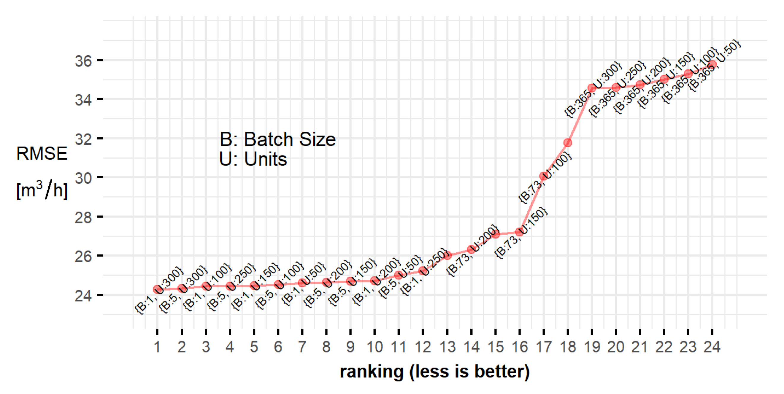
Moreover, two hyperparameters—the batch size and the number of units—were optimized. The former refers to the number of days (samples), each with 24 data points, that the network sees in order to calculate an error and update its weights , whereas the latter defines the dimension of the hidden state vector , that is, n in the equations that describe the LSTM cell of Figure 1, also known as model order.
In preparation for finding optimal values for the number of units and batch size, the data set from use case 1 was selected, setting the following search spaces:
The minimum batch size in the search space is set to one day, whereas the maximum takes the whole year, i.e., 365 days. Note that all selected values for the batch size are factors of 365, allowing the network to be trained with all the samples (days) contained in the validation data set.
Regarding the number of units, the search space was set between 50 and 300 with discrete step size of 50.
Given the small size of the search spaces resulting in 24 combinations of parameters, namely, candidates, it is possible to scan each one in order to see when the best prediction over the validation data is obtained. This brute force algorithm, known as grid search, has a wide range of applications going beyond tuning the hyperparameters of a neural networks. For instance, the reader can find a step-by-step description of the algorithm in [43], where the aim was to find parameters to overfit a previously known function. As far as for the validation strategy, 365 samples (days) were selected for training and 365 samples for validation (see data splits of the LSTM in Batch Learning from Figure 6). This was decided after several trials with 3-fold and 5-fold cross-validation using the train and validation data as one joined data set led to non-stable optimization results, making it so the strategy unreliable even when the order of days and fold sequences were preserved. After running grid search twenty times per combination of hyperparameters and averaging the root mean squared errors (RMSE), that is,
where y is the water flow in the validation data set, is the predicted water flow using the fitted network with the train data set an at hourly time step i and , the ranks of each combination was obtained as depicted below in Figure 5.
In general, keeping low values for the batch size (1 or 5) will yield better results than taking the complete training data as one batch. Regarding the number of units, any selected value from the search space will be able to model the function with enough flexibility, thus generating similarly good results. Finally, a batch size of 5 and 100 units are used for the network’s architecture. Note that these optimized parameters yield the best solution for the validation set, meaning that they may not generate an optimal solution for the test data set. The same architecture was also used to produce the forecasts for use case 2. In this publication, the fitting of the LSTM hyperparameters was performed by taking into account the measurements with the information about the weekday and if it is a work day, national holiday, or the day before a national holiday.
4.2. Evaluation Metric for Model Comparison
For a quantitative comparison of the methods, the root mean square error (RMSE) for each day as well as the RMSE for the whole test data set are calculated. The RMSE for each days is calculated as follows:
with being in our case the 24 h of the daily profile at day j. This describes the size of the test data set, in our case 365 days, is the correct consumption and the model estimate. Validating the performance of the models against the real consumption profiles and against each other is done by using boxplots and by calculating the mean and standard deviation of . During the development of the methods, other performance measures, like mean absolute percentage error (MAPE) or the mean absolute error (MAE), have been taken into account and evaluated. As this led to similar results, they are not considered in this paper.
5. Results for Consumption Profile Prediction
In the following, several methods are used for the prediction of the daily consumption profiles and benchmarked against each other. This quality of the daily consumption prediction can be seen as an important step with regard to the improvement of the pump schedule planning. To compare the individual methods against each other, two scenarios—batch learning, following the traditional approach in machine learning, and online learning—are distinguished from each other. Both scenarios with the used methods are shown in Figure 6. In the following, the results of the two scenarios batch learning and online-learning are described in detail.
5.1. Scenario 1: Batch Learning
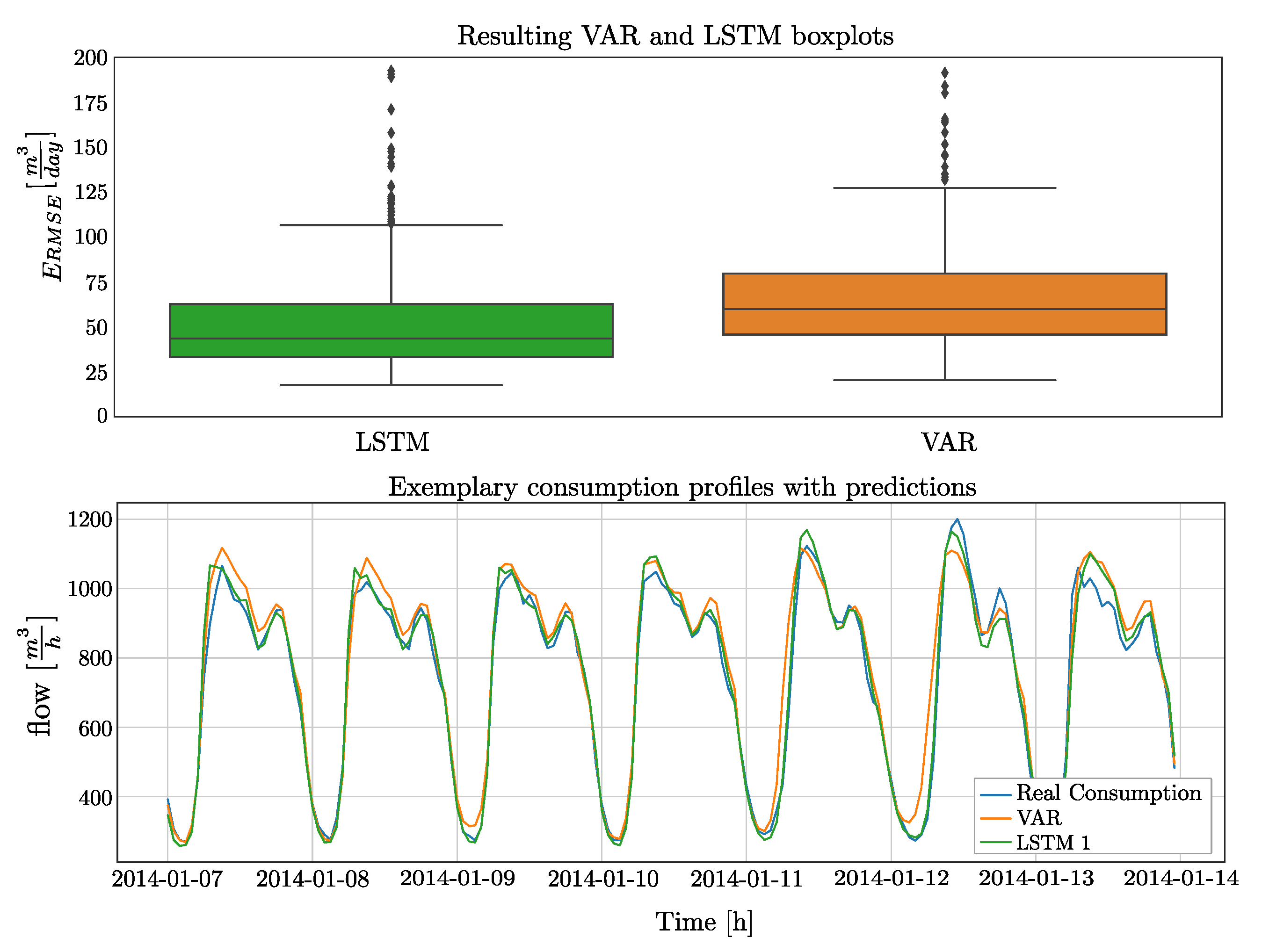
In machine learning, a classic approach means to train a model on historical data and then keeping its parameters unchanged for prediction. Not changing parameters has the advantage that no abnormal behavior like flushing of pipes or pipe breaks are accidentally learned by the model. Still, not updating the model also means that no long-term effects like seasonality can be learned by the model. In the following, the two models VAR and LSTM 1 are initially trained on the data set from use case 1 and then kept constant. The results on the test data set are given in Figure 7 in terms of boxplots. Furthermore, for a better understanding on how the methods behave, the lower plot in Figure 7 shows the daily consumption profile of a randomly selected week.
Regarding the root mean square error, the LSTM 1 achieves an of 48.3 per day, while the VAR performs slightly worse, ending up in a value of 52.3 . Regarding the boxplots, both methods result in a similar interquartile distance of 29.3 (VAR) and 28.5 (LSTM 1) per day. When calculating the mean (and not the median like in the box plots) of LSTM 1 this results in 52.27 and for the VAR in 56.58 per day. To interpret the , in that case this means nothing else then the size by which the models have missed the daily consumption on the average.
Finally, the question arises, why LSTM 1 significantly outperforms the VAR. Therefore, LSTM 1 and VAR were trained again, while removing the weekday and holiday information from the data set. In that case, both methods perform equally well, while the resulting box plots are similar to the one of the VAR in Figure 7. This can be interpreted in the way that during training the VAR neglects the information of the weekday, making the method perform more poorly than the LSTM on the prediction of the week-end consumption profiles. The LSTM, due to its long-term memory, can cope with this information, resulting in a significantly better performance. Of course, it would be possible to develop a heuristic, e.g., by using one VAR for the weekend and one VAR for weekends and national holidays to achieve better results. Still, note that regarding the LSTM, no external logic from the expert is needed as the LSTM can find the heuristic by itself. For the end user, this provides a more comfortable possibility to connect it to different water distribution networks.
5.2. Online Learning
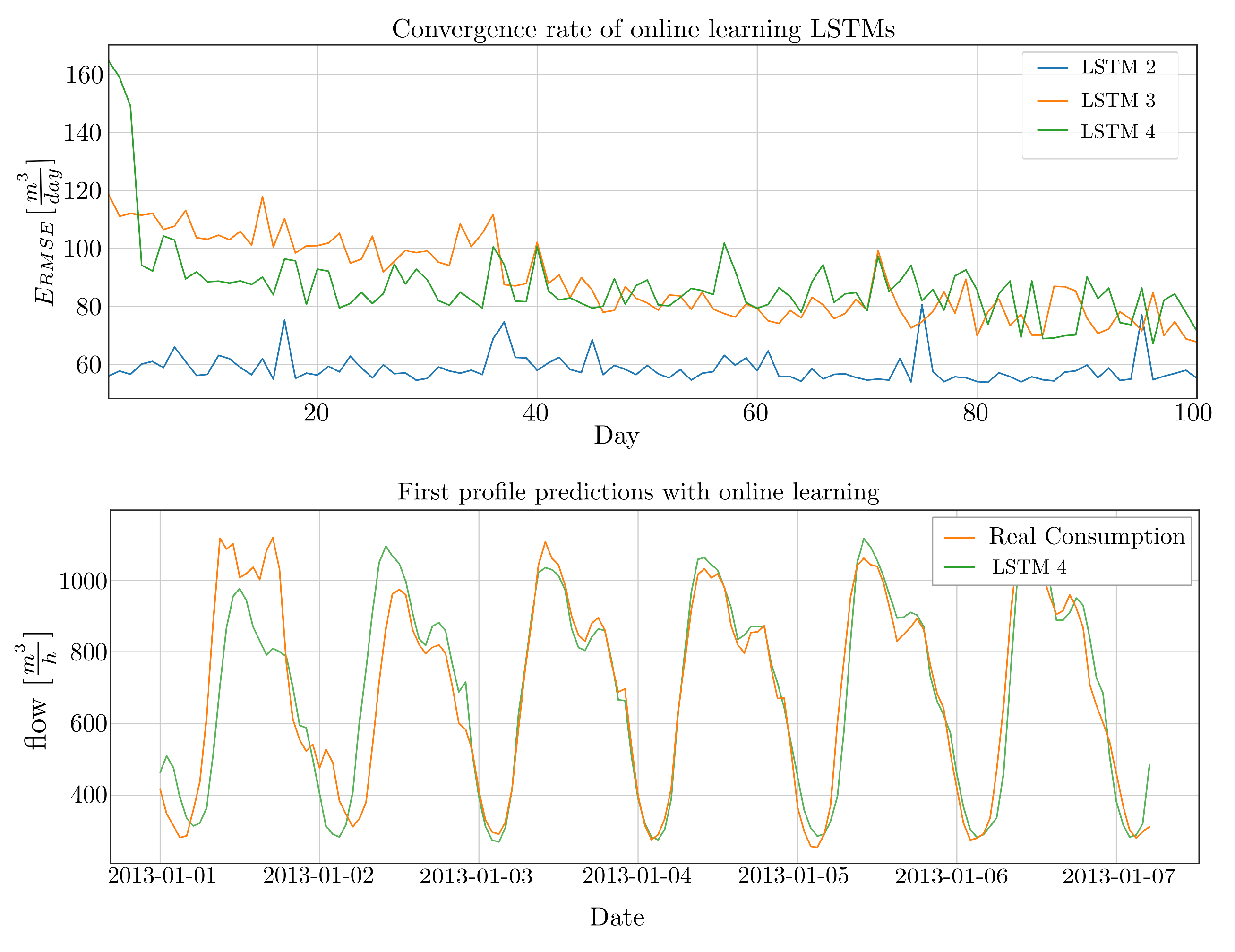
Historical data are not always available for training: for the prediction of a consumption profile, new sensors need to be installed or the cleaning and preparation of historical data is not feasible. Regarding LSTMs, under these circumstances two approaches are possible to train a model every time when a new daily profile is available: (1) Start with an untrained model which only knows the architecture (e.g., how many units and which layers should be used). This model learns to predict the water consumption “on the fly”, meaning that the first couple of predictions will not give reasonable results, but, as more data is available, the better the prediction will be. (2) Take a model from another water distribution network which has a similar behavior. Use this model as a starting point and adapt its hyperparameters through online learning. Furthermore, even when having historical data available, it can also be interesting to perform an online learning on a well fitted LSTM from batch learning (see scenario 1). One of the reasons in this use case is, e.g., if one wants to integrate seasonality into the prediction of the model. In the following, three approaches are compared to each other, one model being pretrained on use case 1 (LSTM 2), another model being pretrained on use case 2 (LSTM 3), and a third model without pretraining (LSTM 4).
The results of all three LSTMs are sketched in Figure 8. The upper plot shows the convergence rate on a daily base on the first 100 days and the lower plot shows an exemplar of the first predicted consumption profiles for model LSTM 4 doing online learning without pretraining.
As one could have expected, LSTM 2 gives the best results. Additionally, the error stays almost constant, meaning that the model parameters are only slightly changing. Investigating the learning process for the two other models gives some more interesting results. First, already after four days, the model without pretraining, LSTM 4, outperforms the model LSTM 3: the transfer learning model does not forget its old state fast enough. After around 40 days, both LSTMs behave similar, slowly converging against LSTM 2.
As mentioned, the lower plot in Figure 8 shows the first six days from LSTM 4. In that case results are remarkable, as the third day (meaning 4 days of training are used) is already predicted quite well. Of course, this model still does not have any information about weekends or national holidays, which leads to a large when testing the LSTM on the complete test data set. Still, especially from an end user point of view, this result is interesting as untrained LSTMs can be connected to distribution plant and deliver reasonable results quite fast.
6. Results for Optimal Pump Control
As a base for the computation of one year of optimal pump control for the water supply system of a city with 100,000 inhabitants, the six different models from the previous sections—four LSTM-models, the naïve predictor, and VAR-model—were used to predict the water consumption of each day. The Naïve predictor, described in the beginning of the paper, has already been implied in field tests in the considered water supply system [42]. Using the described decision support software H2Opt, optimization of the pump operation was done for all prediction models over a period of one year. The simulations were compared to simulations using the third year of use case 1 as realized consumption data together with the optimized pump operation plans. For all prediction models, optimization of the pump operation was possible for 346 out of 365 days of the year. All of the 19 missing days could not be simulated as either the consumption-related data were missing or the software could not handle special occurrences in the waterworks. Therefore, the problems with simulating and optimizing pump operation on these days are independent of the prediction models.
Further on to these days, seven additional days were manually classified as “outliers” (Table 2). These days stand out in that the predicted water consumption of some hours deviates by more than 500 /h from the real data. The reason for the deviations can mainly be found in measurement data, although we do not always know if they are measurement errors (as for 28 April 2014) or especially high or low water consumptions (like pipe breaks, for example). The naïve predictor and VAR, which depend directly on the data prior to prediction, are most sensitive to such non-typical measurement data. This can be seen for example for the day 28 April 2014 which was classified as outlier due to measurement errors in the true data (not shown). However, the following day was only classified as outlier for the two models that use preceding day for prediction on that day, but not for the four LSTM-based models.
Figure 9 and Table 3 summarize the results of the simulations. For the water supplier, it is of importance that a planned schedule remains feasible under the realized water consumption. This means that the storage container of the system must neither overflow nor its content fall below a given threshold of water that is stored for firefighting. When optimizing pump operation with respect to energy efficiency, the pumps are usually operated such that the storage container is often at its lower limit. Therefore, even small deviations of the true water consumption from the prediction used for optimization could lead to infeasibility of the planned pump operation schedule. Table 3 shows that, as far as feasibility is concerned, the LSTM 1 outperforms the other models clearly. It is followed by VAR, LSTM 4, the Naïve predictor, LSTM 2, and LSTM 3.
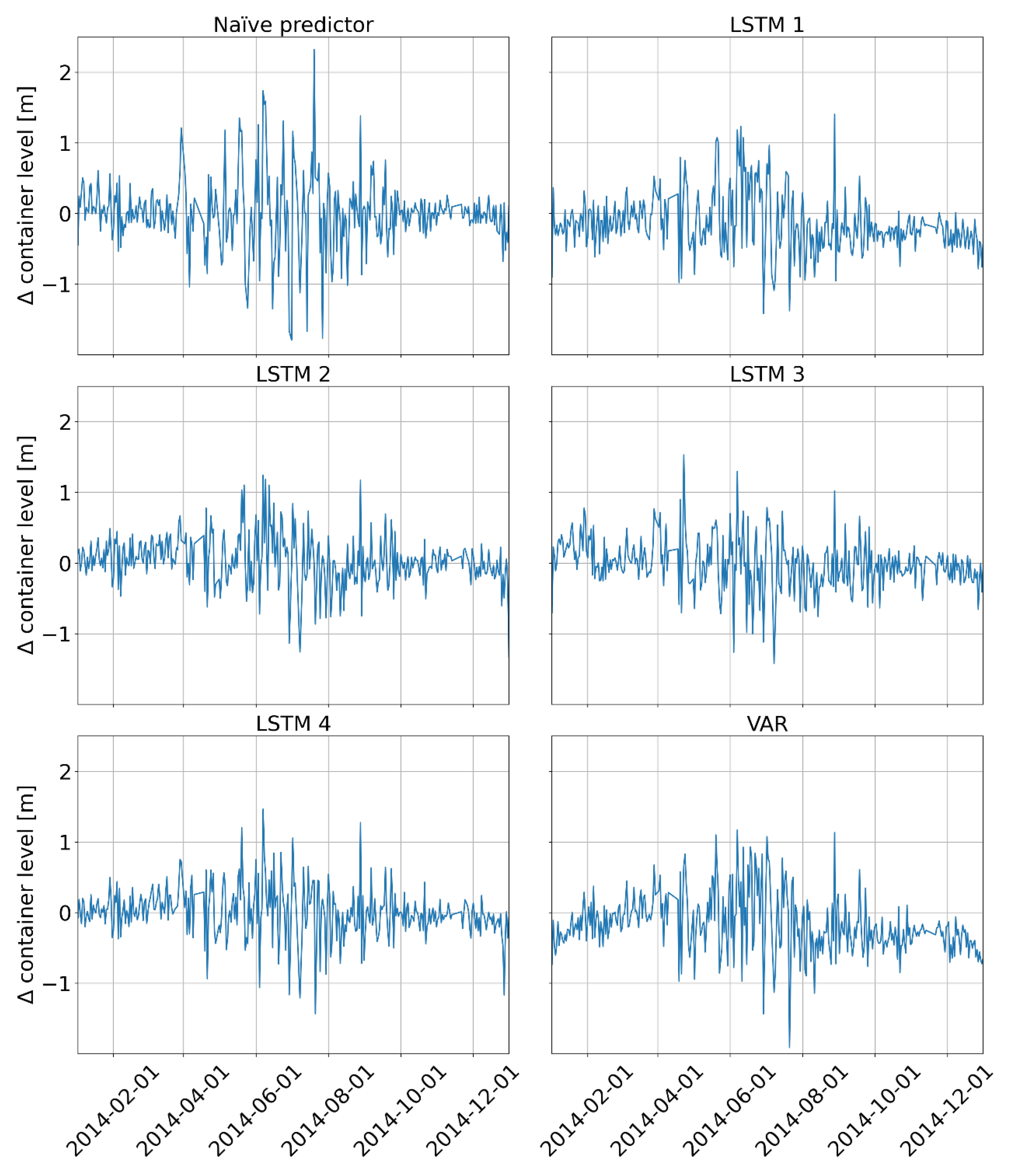
Despite the feasibility of a plan, the end-of-day container level is an important figure for water suppliers to rank the quality of a pump operation schedule, as it is the base for starting the operation planning of the next day. Therefore, the optimization result should be reliable concerning this number. Figure 9 reveals that the optimized end-of-day container levels exhibit some difference to the true value when simulating the optimized pump operation plan under the realized water consumption, i.e., the third year of the use case 1 data. Yet, the variance of the deviations is smaller for the LSTM-based methods and VAR than for the naïve predictor-based optimizations. No matter which variances are looked at (with or without the outliers given in Table 2), there is a clear ranking in performance of this key parameter: The naïve predictor is the worst, followed by VAR and LSTM 1, with at least 1% smaller standard deviation values. In contrast, the models incorporating online learning all perform better in their mean values as well as in standard deviations of end-of-day container level difference. The LSTM-based models 2–4, that all used online learning, show only slight differences: The online (LSTM 2) and transfer learning model (LST) perform a little better than the LSTM without pretraining (LSTM 4). However, the differences are within ±2 cm. This raises hope that even an untrained LSTM model can very soon deliver high quality results. The deviations are larger in summer months, when the water consumption is less uniform from day to day than in winter, and therefore more difficult to predict. During this phase, the online learning LSTMs yield better results than LSTM 1, which is more or less as good as VAR, but still better than the Naïve predictor.
7. Conclusions
In summary, all methods can be used for the definition of pump schedules for the next 24 h. All investigated methods have shown reasonable results for the prediction of the next days consumption profile.
By passing the methods one by one, initially the vector autoregressive model, as a traditional method for time series prediction, achieved the expected results only lacking the possibility to integrate categorical data, like day of the week and national holidays.
The LSTM, being in focus in this paper, was investigated in several points of view. First, it was benchmarked against the VAR. Due to its characteristic to have a long-term memory, it has the possibility to separate different days of the week from each other leading to a better performance compared to the VAR. In a next step, the LSTM has been examined regarding suitability for online learning. In that case, the results are quite promising. Especially the learning rate of the completely untrained LSTM, which only needs a couple of days to achieve reasonable results, should again be emphasized. Using a pretrained model from another network should be done with care as worse results are achieved compared to a completely untrained one. One reason is that the LSTM does not forget its initial parameterization state fast enough and therefore performs worse than a completely untrained one. This leads to the research question whether the LSTM architecture can be adapted appropriately, e.g., by adding a parameterizable forgetting factor into a cell to improve the transfer learning. Another leftover research question is whether the results achieved on this use case (remember use case 2 was only used for pretraining a LSTM) can be generalized to predict consumption profiles from other networks.
Beyond evaluating the prediction models themselves, they were tested in a typical use case: In a one-year-long simulation study, they served as input for optimizing the pump operation of the next day. As benchmark, a naïve predictor model was used, which had already been proven to be valid in several field tests. The results strengthen the trust in the LSTM method which performed very similar or even better than the benchmark in all performance indicators. Especially, the good quality of the LSTM with no pretraining is of interest for small water suppliers that have no capacity to store large amounts of historical data.
Finally, less of a research but more of an IT challenge will be to bring LSTM models into a real production environment. A question that arises in that setting is how to verify that the LSTM is in its working range and does not produce faulty results, e.g., due to some changes in the input data set which it is not informed about.
Author Contributions
Methodology, C.K., H.K., and D.N.; software, validation, and writing, C.K., H.K., N.M.G., and J.A.T.; visualization, C.K. and H.K.; data curation, H.K., D.N., and J.A.T.; supervision, C.K. All authors have read and agreed to the published version of the manuscript.
Funding
This contribution is supported by the Fraunhofer Cluster of Excellence “Cognitive Internet Technologies”, Center for Machine Learning and by the BMBF project W-Net 4.0 (02WIK1477A-E). This research also contributes to the project Copt2 funded by the European Union from the European Regional Development Fund and the State of Rhineland-Palatinate.
Acknowledgments
The authors thank the EWR Netz GmbH for providing their water consumption data, specifically Wolfgang Hausen, the head of Asset Service. The authors also thank their colleagues Julia Nies and Cristina Collicott for reviewing this paper.
Conflicts of Interest
The authors declare no conflict of interest.
References
- Roclawski, H.; Knapp, A.; Geil, C.; Böhle, M.; Krieg, H.; Nowak, D. H2Opt—Eine Software zur Entscheidungsunterstützung für die Planung und den Betrieb von Trinkwasserversorgungsanlagen. Energ. Wasser Prax. 2018, 3, 30–33. [Google Scholar]
- Adhikari, R.; Agrawal, R. An Introductory Study on Time Series Modeling and Forecasting; LAP Lambert Academic Publishing: Düsseldorf, Germany, 2013. [Google Scholar]
- Du, H.; Zhao, Z.; Xue, H. ARIMA-M: A New Model for Daily Water Consumption Prediction Based on the Autoregressive Integrated Moving Average Model and the Markov Chain Error Correction. Water 2020, 12, 760. [Google Scholar] [CrossRef] [Green Version]
- Benitez, R.; Ortiz-Caraballo, C.; Preciado, J.; Conejero, J.; Sanchez, F.; Largo, A. A Short-Term Data Based Water Consumption Prediction Approach. Energies 2019, 12, 2359. [Google Scholar] [CrossRef] [Green Version]
- Sutskever, I.; Vinyals, O.; Le, Q. Sequence to sequence learning with neural networks. Adv. Neural Inf. Process. Syst. 2014, 3104–3112. [Google Scholar]
- Antunes, A.; Andrade-Campos, A.; Sardinha-Lourenço, A.; Oliveira, M.S. Short-term water demand forecasting using machine learning techniques. J. Hydroinform. 2018, 20, 1343–1366. [Google Scholar] [CrossRef] [Green Version]
- Poornima, P.; Boyapati, S. Prediction of Water Consumption Using Machine Learning Algorithm. In ICCCE 2020; Springer: Singapore, 2021; pp. 891–908. [Google Scholar]
- Rahim, M.S.; Nguyen, K.A.; Stewart, R.A.; Giurco, D.; Blumenstein, M. Machine Learning and Data Analytic Techniques in Digital Water Metering: A Review. Water 2020, 12, 294. [Google Scholar] [CrossRef] [Green Version]
- An, A.J.; Chan, C.; Shan, N.; Cercone, N.; Ziarko, W. Applying knowledge discovery to predict water-supply consumption. IEEE Expert Intell. Syst. Appl. 1997, 12, 72–78. [Google Scholar] [CrossRef] [Green Version]
- Arampatzis, G.; Perdikeas, N.; Kampragou, E.; Scaloubakas, P.; Assimacopoulos, D. A water demand forecasting methodology for supporting day-to-day management of water distribution systems. In Proceedings of the 12th International Conference “Protection & Restoration of the Environment, Skiathos Island, Greece, 29 June–3 July 2014. [Google Scholar]
- Mamo, T.G.; Juran, I.; Shahrour, I. Urban Water Demand Forecasting Using the Stochastic Nature of Short Term Historical Water Demand and supply Pattern. J. Water Resour. Hydraul. Eng. 2013, 2, 92–103. [Google Scholar]
- Adamowski, J.K.; Christina Comparison of Multivariate Regression and Artificial Neural Networks for Peak Urban Water-Demand Forecasting. Evaluation of Different ANN Learning Algorithms. J. Hydrol. Eng. 2010, 15, 729–743. [Google Scholar] [CrossRef] [Green Version]
- Bougadis, J.; Adamowski, K.; Diduch, R. Short-term municipal water demand forecasting. Hydrol. Process. 2005, 19, 137–148. [Google Scholar] [CrossRef]
- Candelieri, A.; Soldi, D.; Archetti, F. Short-term forecasting of hourly water consumption by using automatic metering readers data. Procedia Eng. 2005, 119, 844–853. [Google Scholar] [CrossRef]
- Manuel, H.; Luís, T.; Joaquín, I.; Rafael, P. Predictive models for forecasting hourly urban water demand. J. Hydrol. 2010, 387, 141–150. [Google Scholar]
- Rangel, H.R.; Puig, V.; Farias, R.L.; Flores, J.J. Short Term Demand Forecast using a Bank of Neural Network Models Trained using Genetic Algorithms for the Optimal Management of Drinking Water Networks. J. Hydroinform. 2016, 19, 1–16. [Google Scholar] [CrossRef] [Green Version]
- Perez, R.; Kivalov, S.; Schlemmer, J.; Hemker, K.; Renn, D.; Hoff, T.E. Validation of short and medium term operational solar forecasts in the US. Sol. Energy 2010, 84, 2161–2172. [Google Scholar] [CrossRef]
- Takeyosi, K. Prediction of photovoltaic power generation output and network operation. Integr. Distrib. Energy Resour. Power Syst. 2016, 15–20. [Google Scholar] [CrossRef]
- Kaushik, S.; Choudhury, A.; Sheron, P.; Dasgupta, N.; Natarajan, S.; Pickett, L.; Dutt, V. AI in Healthcare: Time-Series Forecasting Using Statistical, Neural, and Ensemble Architectures. Front. Big Data 2020, 3, 4. [Google Scholar] [CrossRef] [Green Version]
- Shen, Y.; Giannakis, G.B.; Baingana, B. Nonlinear Structural Vector Autoregressive Models with Application to Directed Brain Networks. IEEE Trans. Signal Process. 2019, 67, 5325–5339. [Google Scholar] [CrossRef] [PubMed]
- Melnyk, I.; Matthews, B.; Valizadegan, H.; Banerjee, A.; Oza, N. Vector autoregressive model-based anomaly detection in aviation systems. Procedia Eng. 2015, 119, 442–449. [Google Scholar] [CrossRef] [Green Version]
- Demir, E.; Gozgor, G.; Lau, C.; Vigne, S. Does economic policy uncertainty predict the Bitcoin returns? An empirical investigation Financ. Res. Lett. 2018, 26, 145–149. [Google Scholar] [CrossRef] [Green Version]
- Konar, A.; Bhattacharya, D. Time-Series Prediction and Applications: A Machine Intelligence Approach, Intelligent Systems Reference Library; Springer International Publishing: Berlin, Germany, 2017. [Google Scholar]
- Hochreiter, S.; Schmidhuber, J. Long short-term memory. Neural Comput. 1997, 9, 1735–1780. [Google Scholar] [CrossRef]
- Carbune, V.; Gonnet, P. Fast multi-language LSTM-based online handwriting recognition. Int. J. Doc. Anal. Recognit. 2020, 1–14. [Google Scholar] [CrossRef] [Green Version]
- He, T.; Droppo, J. Exploiting LSTM Structure in Deep Neural Networks for Speech Recognition. In Proceedings of the 2016 IEEE International Conference on Acoustics, Speech and Signal Processing (ICASSP), Shanghai, China, 20–25 March 2016. [Google Scholar]
- Li, J.; Zhao, R.; Sun, E.; Wong, J.H.; Das, A.; Meng, Z.; Gong, Y. High-Accuracy and Low-Latency Speech Recognition with Two-Head Contextual Layer Trajectory LSTM Model. In Proceedings of the IEEE International Conference on Acoustics, Speech and Signal Processing (ICASSP), Barcelona, Spain, 12 October 2020; pp. 7699–7703. [Google Scholar]
- Yang, H.; Ding, K.; Qiu, R.C.; Mi, T. Remaining Useful Life Prediction Based on Normalizing Flow Embedded Sequence-to-Sequence Learning. IEEE Trans. Reliab. 2020. [Google Scholar] [CrossRef]
- Chimmula, V.K.R.; Zhang, L. Time series forecasting of COVID-19 transmission in Canada using LSTM networks. Chaos Solitons Fractals 2020, 135, 109864. [Google Scholar] [CrossRef] [PubMed]
- Xiang, Z.; Yan, J.; Demir, I. A Rainfall-Runoff Model With LSTM-Based Sequence-to-Sequence Learning. Water Resour. Res. 2020, 56, 1. [Google Scholar] [CrossRef]
- Elsheikh, A.; Katekar, V.; Muskens, O. Utilization of LSTM neural network for water production forecasting of a stepped solar still with a corrugated absorber plate. Process. Saf. Environ. Prot. 2021, 148, 273–282. [Google Scholar] [CrossRef]
- Barzegar, R.; Aalami, M.T.; Adamowski, J. Short-term water quality variable prediction using a hybrid CNN–LSTM deep learning model A Short-Term Data Based Water Consumption Prediction Approach. Stoch. Environ. Res. Risk Assess. 2020, 1–19. [Google Scholar] [CrossRef]
- Xu, Z.; Ying, Z.; Li, Y.; He, B.; Chen, Y. Pressure prediction and abnormal working conditions detection of water supply network based on LSTM. Water 2020, 3, 963–974. [Google Scholar] [CrossRef]
- Olah, C. Understanding LSTM. Available online: Http://colah.github.io/posts/2015-08-Understanding-LSTMs/ (accessed on 22 October 2020).
- Zilka, L.; Jurcicek, F.; Guruprasad, N.; Gerber, J.; Carlson, K. Predict Land Covers with Transition Modeling and Incremental Learning. In Proceedings of the International Conference on Data Mining (SIAM), Houston, TX, USA, 27–29 April 2017; pp. 171–179. [Google Scholar]
- Xiaowei, J.; Khandelwal, A. Incremental LSTM-based dialog state tracker. In Proceedings of the 2015 Ieee Workshop on Automatic Speech Recognition and Understanding (Asru), Scottsdale, AZ, USA, 13–17 December 2015; pp. 757–762. [Google Scholar]
- Lee, J.; Dernoncourt, F.; Szolovits, P. Transfer learning for named-entity recognition with neural networks. arXiv 2017, arXiv:1705.06273. [Google Scholar]
- Coutinho, E.; Deng, J.; Schuller, B. Transfer learning emotion manifestation across music and speech. In Proceedings of the International Joint Conference on Neural Networks (IJCNN), Beijing, China, 6–11 July 2014; pp. 3592–3598. [Google Scholar]
- Luna, T.; Ribau, J.; Figueiredo, D.; Alves, R. Improving energy efficiency in water supply systems with pump scheduling optimization. J. Clean. Prod. 2019, 213, 342–356. [Google Scholar] [CrossRef]
- Marchi, A.; Simpson, A.; Lambert, M. Pump Operation Optimization Using Rule-based Controls. Procedia Eng. 2017, 186, 210–217. [Google Scholar] [CrossRef]
- Mala-Jetmarova, H.; Sultanova, N.; Savic, D. Lost in Optimisation of Water Distribution Systems? A Literature Review of System Operation. Environ. Model. Softw. 2017, 93, 209–254. [Google Scholar] [CrossRef] [Green Version]
- Krieg, H.; Nowak, D.; Bortz, M.; Knapp, A.; Geil, C.; Roclawski, H.; Böhle, M. Decision support for planning and operation of drinking water supply systems. Water Solut. 2018, 3, 49–60. [Google Scholar]
- Thomas, J.A. Optimisation Method for the Clear Sky PV Forecast Using Power Records from Arbitrarily Oriented Panels. In Proceedings of the 2018 7th International Conference on Renewable Energy Research and Applications (ICRERA), Paris, France, 14–17 October 2018; pp. 117–123. [Google Scholar]
Figure 1.
Basic architecture of a long short-term memory network according to Olah [34]).
Figure 1.
Basic architecture of a long short-term memory network according to Olah [34]).

Figure 2.
Scheme of the water supply system used for benchmarking. This figure is taken from the work in [42] and is slightly modified.
Figure 2.
Scheme of the water supply system used for benchmarking. This figure is taken from the work in [42] and is slightly modified.

Figure 3.
Daily workflow of the operator using the decision supporting software H2Opt.

Figure 4.
Mean daily consumption profiles with standard deviation from the use cases for the seven days of the week day.
Figure 4.
Mean daily consumption profiles with standard deviation from the use cases for the seven days of the week day.

Figure 5.
Ranking of hyperparameters combinations. Each point represents the average of the twenty RMSE calculations.
Figure 5.
Ranking of hyperparameters combinations. Each point represents the average of the twenty RMSE calculations.

Figure 6.
Used scenarios for benchmarking the performance of the different methods.

Figure 7.
Upper plot: Resulting boxplots when performing batch learning using a VAR and LSTM model. Lower plot: Exemplary predicted daily profiles for water consumption profiles for one week.
Figure 7.
Upper plot: Resulting boxplots when performing batch learning using a VAR and LSTM model. Lower plot: Exemplary predicted daily profiles for water consumption profiles for one week.

Figure 8.
Results of online learning using three types of LSTMs. Upper plot: convergence of the different LSTMS. Lower plot: First predicted consumption profiles from the LSTM doing online learning “on the fly”.
Figure 8.
Results of online learning using three types of LSTMs. Upper plot: convergence of the different LSTMS. Lower plot: First predicted consumption profiles from the LSTM doing online learning “on the fly”.

Figure 9.
Differences in end-of-day container levels between pump operation optimization using predicted water consumption and simulating the optimized pump operation plan with the realized water consumption. The outliers given in Table 2 are excluded.
Figure 9.
Differences in end-of-day container levels between pump operation optimization using predicted water consumption and simulating the optimized pump operation plan with the realized water consumption. The outliers given in Table 2 are excluded.


Table 1.
Summary of datasets.
| Label | Use Case 1 | Use Case 2 |
|---|---|---|
| Measurement | Flow in | Flow in |
| Sampling Rate | 1 h | 1 h |
| Total Days | 1095 | 335 |
| Days for Training | 365 | 113 |
| Days for Validation | 365 | 111 |
| Days for Test | 365 | 111 |
Table 2.
Results: Outliers. Days that are manually classified as outliers due to high deviations in water consumption prediction from true water consumption.
Table 2.
Results: Outliers. Days that are manually classified as outliers due to high deviations in water consumption prediction from true water consumption.
| Day | Naïve Predictor | LSTM 1 | LSTM 2 | LSTM 3 | LSTM 4 | VAR |
|---|---|---|---|---|---|---|
| 2014-4-28 | x | x | x | x | x | x |
| 2014-4-29 | x | x | ||||
| 2014-6-29 | x | |||||
| 2014-7-4 | x | x | ||||
| 2014-7-6 | x | |||||
| 2014-7-21 | x | |||||
| 2014-12-31 | x |
Table 3.
Results of optimal pump control. Rows 1–3 show the results concerning feasibility of the simulation and the predictions of the consumption. Rows 4–7 show the mean end-of-day container level differences between the simulations using predicted consumption and realized consumptions for the whole year (row 4–5) and the summer months (rows 6–7) either with or without the outliers from line 3 and Table 2. Each cell in row 4–7 contains four entries: the mean and standard deviation of the absolute container level differences in meters and their representations in percentage of total container height. Bold values: lowest and highest variance in percentage of container level deviations.
| Naïve Predictor | LSTM 1 | LSTM 2 | LSTM 3 | LSTM 4 | VAR | ||
|---|---|---|---|---|---|---|---|
| Optimized days | days | 346 | 346 | 346 | 346 | 346 | 346 |
| Feasible days after re-simulation | days | 228 | 287 | 215 | 209 | 240 | 270 |
| (65.9%) | (82.9%) | (62.1%) | (60.4%) | (69.4%) | (78.0%) | ||
| Additional outliers | days | 5 | 2 | 1 | 1 | 2 | 3 |
| End-of-day container level differences | |||||||
| All days | m | ||||||
| % | |||||||
| All days without additional outliers | m | ||||||
| % | |||||||
| April-September | m | ||||||
| % | |||||||
| April-September without additional outliers | m | ||||||
| % | |||||||
Publisher’s Note: MDPI stays neutral with regard to jurisdictional claims in published maps and institutional affiliations. |
© 2021 by the authors. Licensee MDPI, Basel, Switzerland. This article is an open access article distributed under the terms and conditions of the Creative Commons Attribution (CC BY) license (http://creativecommons.org/licenses/by/4.0/).
Share and Cite
MDPI and ACS Style
Kühnert, C.; Gonuguntla, N.M.; Krieg, H.; Nowak, D.; Thomas, J.A. Application of LSTM Networks for Water Demand Prediction in Optimal Pump Control. Water 2021, 13, 644. https://doi.org/10.3390/w13050644
AMA Style
Kühnert C, Gonuguntla NM, Krieg H, Nowak D, Thomas JA. Application of LSTM Networks for Water Demand Prediction in Optimal Pump Control. Water. 2021; 13(5):644. https://doi.org/10.3390/w13050644
Chicago/Turabian StyleKühnert, Christian, Naga Mamatha Gonuguntla, Helene Krieg, Dimitri Nowak, and Jorge A. Thomas. 2021. "Application of LSTM Networks for Water Demand Prediction in Optimal Pump Control" Water 13, no. 5: 644. https://doi.org/10.3390/w13050644
Note that from the first issue of 2016, this journal uses article numbers instead of page numbers. See further details here.