Resilience Assessment of Water Quality Sensor Designs under Cyber-Physical Attacks

Abstract

Water distribution networks (WDNs) are critical infrastructure for the welfare of society. Due to their spatial extent and difficulties in deployment of security measures, they are vulnerable to threat scenarios that include the rising concern of cyber-physical attacks. To protect WDNs against different kinds of water contamination, it is customary to deploy water quality (WQ) monitoring sensors. Cyber-attacks on the monitoring system that employs WQ sensors combined with deliberate contamination events via backflow attacks can lead to severe disruptions to water delivery or even potentially fatal consequences for consumers. As such, the water sector is in immediate need of tools and methodologies that can support cyber-physical quality attack simulation and vulnerability assessment of the WQ monitoring system under such attacks. In this study we demonstrate a novel methodology to assess the resilience of placement schemes generated with the Threat Ensemble Vulnerability Assessment and Sensor Placement Optimization Tool (TEVA-SPOT) and evaluated under cyber-physical attacks simulated using the stress-testing platform RISKNOUGHT, using multidimensional metrics and resilience profile graphs. The results of this study show that some sensor designs are inherently more resilient than others, and this trait can be exploited in risk management practices.

1. Introduction

Water distribution networks (WDNs) are spatially large and complex systems supplying drinking water to consumers by satisfying multiple objectives, such as maintaining adequate hydraulic pressure, storing water for firefighting, maintaining disinfectant residuals to limit microbial regrowth, and minimizing potential harmful concentrations of substances in the water [1]. Because the requirement of clean drinking water is of utmost importance to public health and societal welfare, WDNs are considered to be critical infrastructure [2]. Indeed, various incidents showcase that severe public hazard, including serious illnesses and deaths and other sociopolitical impacts (e.g., great economic loss), can be the outcome of contamination events in WDNs. Notable incidents include the 1993 cryptosporidium outbreak in Milwaukee [3,4,5], the 2014 Elk River 4-methylcyclohexanemethanol (MCHM) spill in West Virginia [6], the 2016 Beijing misconnection of reclaimed and drinking water pipes, the 2016 lead contamination of Hong Kong’s water system [7], the 2019 Askøy water supply system campylobacter outbreak, and the 2019 E. coli outbreak in Long Beach [8].

Due to the distributed size of WDNs even for smaller settlements, and the practical difficulty of protecting the numerous potential contamination entry points, the policy discourse is concerned with the safety of such systems under various threats. These can stem from deliberate, negligent, or accidental actions [9,10,11], including terrorism [10,12,13,14,15]. Of growing interest is the special case of cyber-physical threats in the form of cyber-physical attacks (e.g., [16,17,18,19,20,21]) where, for example, a deliberate contamination event (a physical attack) is combined with a cyber-attack on the water quality (WQ) monitoring system of the WDN, usually a sub-system of the main SCADA (supervisory control and data acquisition) system.

SCADA systems typically employ central hosts, i.e., a server with a human–machine interface (HMI) and a historian (database computer), and field devices, i.e., remote terminal units (RTUs)/programmable logic controllers (PLCs), actuators, and sensors, connected via communication protocols. These components form the cyber layer of a cyber-physical system (CPS) that interacts in real time with the physical processes with feedback loops [22]. Practically all modern WDNs are CPSs, employing a wide variety of sensors for monitoring the system. Among other properties of the hydraulic processes, e.g., tank level, delivery pressure, flow rate, etc., sensors can be used to monitor water quality in a WDN. The water quality sensors form a subset of the cyber layer responsible for contamination monitoring, which is part of a contaminant warning system (CWS). The information acquired by WQ sensors is subsequently used for mitigation measures such as preventing contamination spread, issuing alarms to the public, and flushing the contaminant out of the network [23].

Naturally, there is a variety of technical challenges to be addressed with every design of CWS [24], notably regarding two main aspects: (a) optimal placement of a limited number of sensors, as it is cost-prohibitive to deploy them (ideally) at all possible locations (nodes) in the network [25], and (b) the effectiveness of continuous real-time online water quality sensors in detecting a contamination event by using surrogate measurements of physiochemical parameters of water to identify anomalies and thus report a contamination [26,27]. The latter is a chemical engineering issue, so researchers in the water sector analyze the sensor design from a civil engineering perspective, aiming at the best (i.e., performance versus cost) topological placement in the WDN, as it is common in the literature to assume “perfect” sensors [24], i.e., sensors with 100% reliability in measuring the WQ parameters at the monitored node (there are studies that also consider non-perfect sensors, e.g., [28]). The optimization of sensor placement is a well-researched topic with numerous publications on optimization strategies, algorithms, and objective functions (e.g., [28,29,30,31,32,33,34,35,36,37]).

However, the resilience of such sensor designs under failure regarding the CWS goal to maintain a level of protection for the WDN is still an under-investigated topic, as recently reported by [31], despite some efforts in previous studies and identifying that structural and communication failures as well as measurement errors are common in water quality sensors (e.g., [38,39]). Moreover, to the authors’ knowledge, a holistic view of WDNs as cyber-physical systems accounting also for failures (e.g., due to cyber-attacks) in the cyber domain (i.e., control, communication, and monitoring) is still in its infancy. Only recently have questions been raised regarding the cyber-physical resilience aspect of such systems (e.g., [40,41]). In addition, software platforms able to stress-test WDN CPSs under cyber-physical attacks have only recently been developed. Such tools include epanetCPA [17] and RISKNOUGHT [19]. WQ cyber-physical simulation, i.e., simulating the complete feedback loops between a CWS, other hydraulic controls of the SCADA, and the real physical hydraulic and contaminant fate processes were made possible for the first time with the recent expansion of RISKNOUGHT [42].

In this work we present a methodology for the resilience assessment of sensor designs under cyber-physical attacks. The attacks comprise the deliberate action of backflow injection of a contaminant into the WDN (a physical attack by overcoming the network’s pressure at an outlet to inject a contaminant) and combinations with cyber-attacks to hinder the CWS’s ability to detect and mitigate the contamination. The assessment is performed using an operational resilience definition by [43] and the RISKNOUGHT stress-testing platform to simulate the scenarios.

2. Sensor Design Resilience Assessment Methodology and Cyber-Physical Tools

2.1. Resilience Assessment

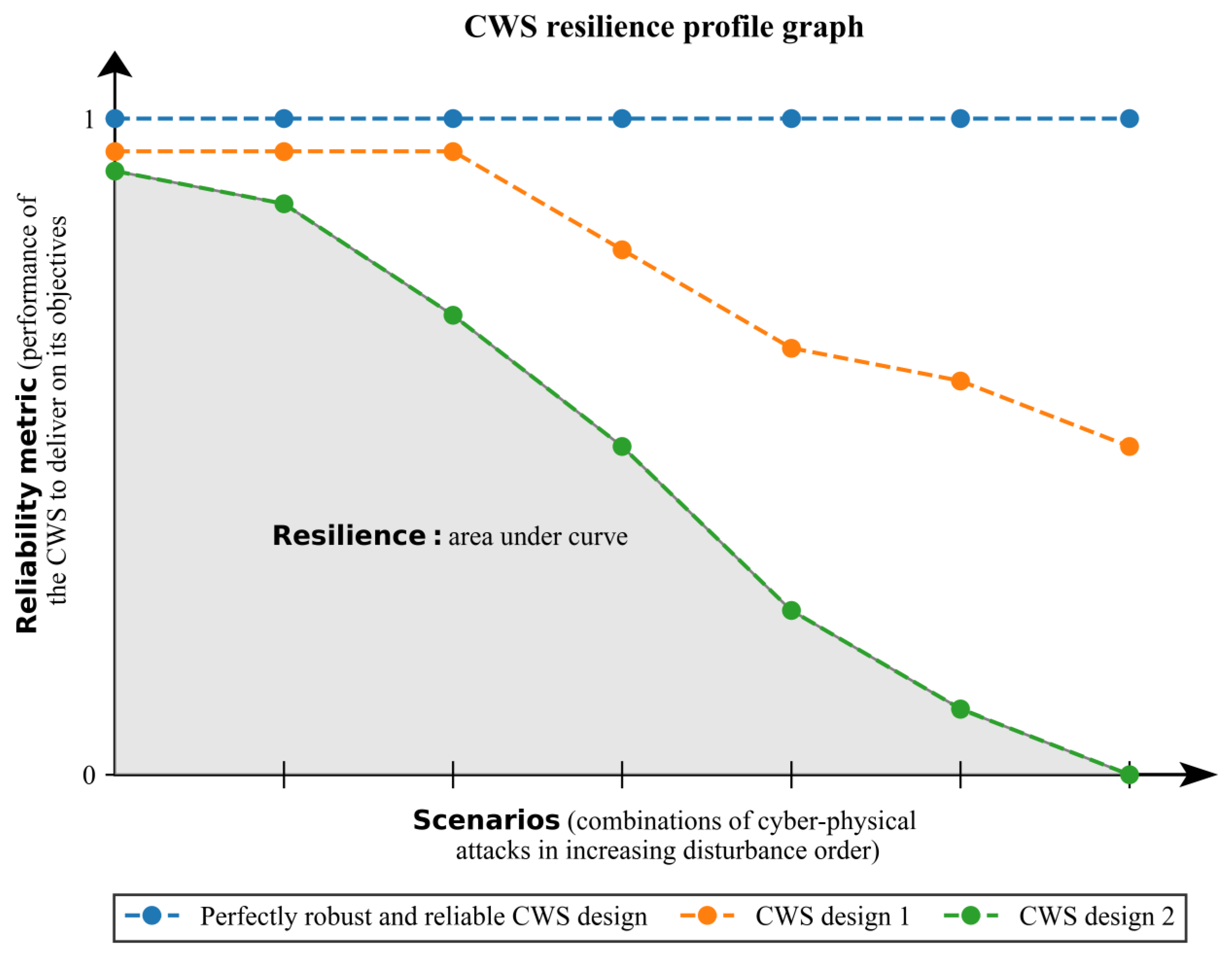
The concept of resilience originally stems from an ecological system’s ability to persist stress [44] and has since been applied in engineering systems with different interpretations in literature, mainly revolving around “continuity and efficiency of system function during and after failure” [45] with various definitions, e.g., [46,47,48]. We use an operational definition where resilience is defined as “the degree to which an urban water system continues to perform under progressively increasing disturbance”, whereas robustness is best defined as “the level of pressure that the system can sustain without failing (or without performance loss)” [43]. With this definition, special types of curves, termed “resilience profile graphs,” communicate the performance of the system to meet its objectives on the y-axis as measured by a metric of reliability, whereas on the x-axis ticks lie scenarios of increasing disturbance and is by definition an ordinal scale. Note that these disturbances extend from stresses within design standards to stresses well beyond design standards. Resilience for a given design is the area under the curve i.e., the integral of reliability over the ordinal scale of scenarios. To scale resilience from 0 to 1, we compare this area to the area of a totally reliable and robust design for all scenarios [43].

To adapt the methodology for the CPS system’s CWS performance under cyber-physical attacks, we use a resilience profile graph as shown in Figure 1. The figure demonstrates the performance of an ideal, perfectly robust, reliable, and resilient CWS design, as well as two others with different properties. In this example, CWS design 1 is more resilient than CWS design 2, as communicated by the respective areas under their reliability curves. CWS design 1 retains higher reliability with the progressive increase in stress from the scenarios, whereas CWS design 2 rapidly loses performance as stress increases. The scenarios represent combinations of cyber-physical attacks that hinder the CWS’s ability to detect contamination while the WDN water is deemed unsafe for consumption. The CWS designs refer to different topologies of placed sensors (different total number and locations monitored) and sets of controls for response and mitigation measures. The reliability metric could be any metric that can describe the CWS performance and the impact on the WDN in a systematic way, such as the detection rate of contamination events.

2.2. Cyber-Physical Simulation Platform

RISKNOUGHT is a cyber-physical stress-testing simulation platform that simulates WDNs as integrated CPSs. This is achieved by coupling two interacting models with feedback loops: (a) the cyber model, a customizable SCADA layer that simulates the control logic and behavior of PLCs, sensors, and actuators, and (b) the physical model, a custom WDN simulator that leverages the WNTR [35] package (version 0.3 at time of writing) to implement pressure-driven analysis (PDA) [49] and quality simulations using the recent EPANET version 2.2 solver [50]. The RISKNOUGHT model is described in detail in [19], whereas the analysis of WQ cyber-physical simulation is presented in [42]. In the stepwise simulation, the physical layer feeds input data (e.g., tank level, concentration of contaminant at nodes, etc.) from the hydraulic and quality simulation to the cyber layer, which uses the information to resolve statements of the deployed control logic schemes and then passes decisions to the physical layer, affecting the hydraulic state for the subsequent simulation step (e.g., open a pump, close a valve, etc.). With regard to the implementation of control logic to facilitate response and mitigation measures against contamination events, RISKNOUGHT enables the use of district metered area (DMA) isolation commands via isolation valves to minimize the extent of the contamination and activation of flushing units to remove the contaminant from the system. As such, RISKNOUGHT can simulate the impact of contamination events even after being detected and enforcing response measures. The platform incorporates a cyber-physical attack model that simulates a variety of cyber-attacks on cyber elements (e.g., denial of service (DoS) attacks, sensor data manipulation, etc.) and physical attacks on elements of the WSN (such as backflow contaminant injections, destruction of pipes, etc.) in stress-testing scenarios.

2.3. Generation of Sensor Designs

In order to generate different topologies of sensor designs, we use TEVA-SPOT [51], a well-known software utilized for sensor placement optimization and the assessment of consequences of contamination events in large WDNs. TEVA-SPOT can employ a wide range of objective functions in sensor placement also common in other works in literature, including the time to detection [29], extent of contamination (total length of contaminated pipes) [52], number of failed detections [52] (which is similar to the inverse of detection likelihood [53]), volume of contaminated water consumed, mass of contaminant consumed [54], and population exposed [52], with the ability to differentiate between population killed and population receiving a specific dose and above. TEVA-SPOT also ranks the sensors deployed from a specific optimization scheme from most to least important in terms of reduced impact of contamination events due to its presence. It should be noted that TEVA-SPOT estimates impact based on the assumption that when a contamination is detected, mitigation and response measures will follow, but the software has no means to actually simulate them, other than providing a specified response time. Therefore, other sensor placement optimization tools could also be considered for the generation of sensor designs, such as Chama [55].

2.4. Cyber-Physical Attack Scenarios

2.4.1. Selecting Cyber-Attack Scenarios

For proper resilience assessment and stress-testing, a scenario set of increasing pressure from scenario to scenario should be constructed. As the focus of this work is to assess the resilience of different sensor topologies against contamination attacks and cyber-physical attacks, the increased stress is translated to progressively more sensors being cyber-attacked. Due to the immense topological, hydraulic, and control complexity of large WDNs, standardization is difficult, as different sensor designs differ in WDN coverage and control sets, thus varying wildly in performance during failure. For normalization reasons, the control sets for response and mitigation measures are similar for every sensor design, i.e., we use isolation commands that cut off connections between all DMAs to stop the contamination spread and activate flushers in all DMAs from where the detected contamination event could have originated. Note that demands on nodes remain unaffected, i.e., are not reduced to zero, to represent consumer compliance to a do-not-use warning. This could be used as another rule but is not dependent upon the system’s control logic rather than consumers’ behavior, and we want to avoid the overhead of changing the network’s properties during runtime. The cyber-attacks have similar attributes i.e., sensor data manipulation to report normal water quality readings masking the contamination, and to negate the effect of temporal hydraulic variance in detection capability, the cyber-attacks happen from simulation start to end for all scenarios and combinations. To choose which sensor to add to the attacked sensors set in a progressive manner, the TEVA-SPOT ranking is used. Therefore, the least stressful scenario contains a single attack on the most important sensor of the topology, then the second most important sensor is also attacked, and so on, with the worst scenario including attacks on all sensors.

2.4.2. Sampling Contaminant Injection Locations

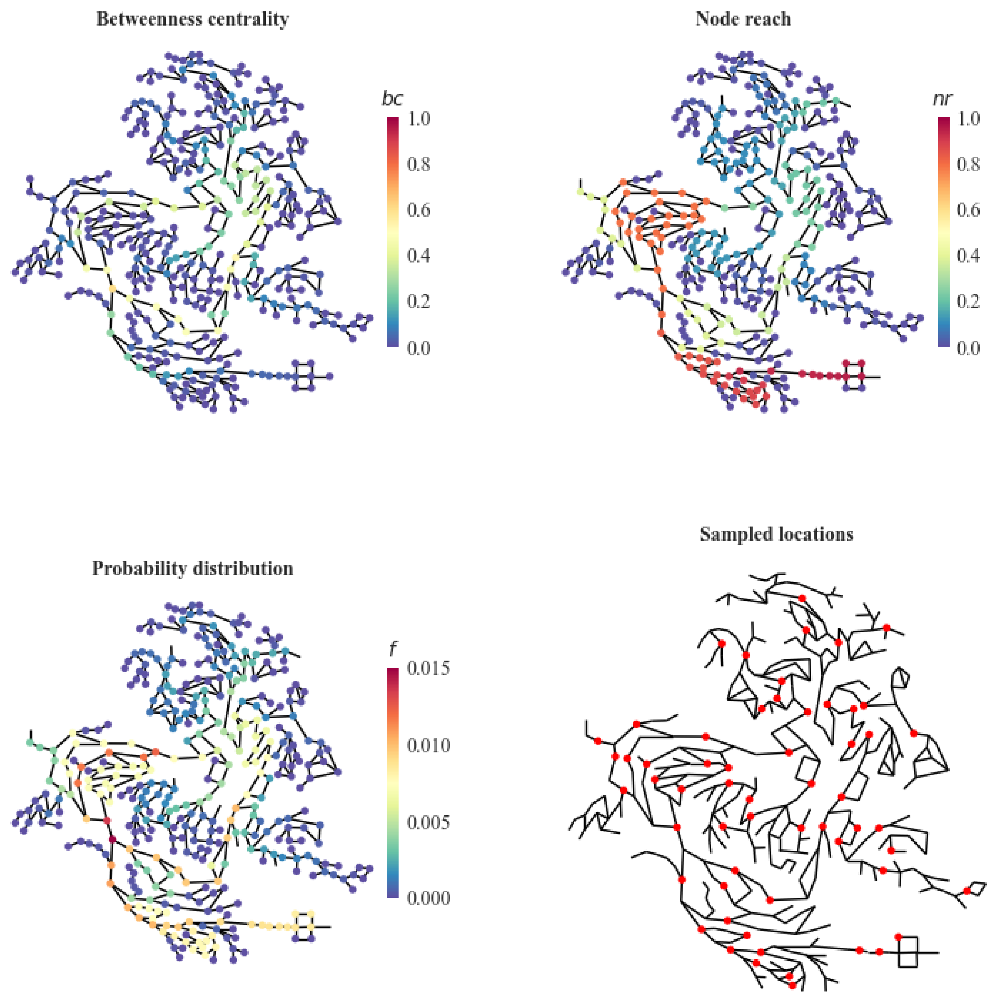
Because of WDN complexity, a single physical attack combined with a cyber-physical attack scenario cannot capture the general expected impact of cyber-physical attacks, as this injection may happen at a still adequately monitored part of the WDN and have a low impact or on the contrary have a large impact if it coincides with an important part of the WDN’s CWS being cyber-attacked. In addition, some injection locations are inherently more topologically critical in terms of reaching other parts of the network, whereas others may pertain only to small branches of the WDN, limiting the impact despite being unnoticed by the CWS. Thus, it is imperative to combine the scenarios with a multitude of different injection locations to calculate the expected outcome of the cyber-physical attacks. Although ideally all injection locations should be considered, the computational time for all the combinations increases drastically. The computational budget may allow for a small number of examined injection locations, so we propose the use of a weighted random choice of nodes from the network, with probabilities of choice not uniform but according to the “fitness” $f_i$ of the node $i$ as an injection location. In this work, we use two metrics, equally weighted to calculate $f_i$. The node betweenness centrality ($bc$) [56] is a metric that is also used to optimally place sensors topologically without hydraulic simulations [57,58] (among other centrality metrics and weighted variations of them by characteristics such as diameters of pipes, etc., which could also be used here). The betweenness centrality $b{c}_i$ for each node $i$ is calculated as

$$b{c}_i={\displaystyle \sum }_{w,e\in I}\frac{\sigma \left(w,e|i\right)}{\sigma \left(w,e\right)}$$

(1)

where $I$ is the set of discrete node elements, $s$ and $e$ are pairs of network nodes, $\sigma \left(w,e\right)$ is the number of shortest $\left(w, e\right)$ paths, and $\sigma \left(w,e|i\right)$ is the number of those paths passing through node $i$. A higher value signifies nodes that are more central, in the sense of residing along more of the shortest path between pairs of other nodes. This metric conveys the expected probability for a node to be along the pathway of a contamination spread from any source point to others, and so topologically lower values will be assigned to nodes residing in smaller branches of the network and higher values along the main water pipes. Because tanks and sources in a water distribution graph representation reside in branches, the second metric considers the actual hydraulic traceability of each location and is calculated from trace simulations in EPANET. These trace simulations are fast, as there is no cyber-physical coupling, and, if required for large networks, a much coarser simulation timestep can be used. After performing a trace quality simulation for each node $i$, we can obtain $p_{ijt}$, which is the percentage of water originating from $i$ for each other node $j$ and for each timestep $t \in \left\{1,m\right\}$, where $m$ is the number of simulation steps. With $n$ being the number of nodes (i.e., the cardinality of set $N$), the node reach $n{r}_i$ can be calculated as

$$n{r}_i=\frac{{{\displaystyle \sum }}_{\forall i\in I}{P}_{ij}}{n}$$

(2)

where

$$P_{ij} = \{\begin{array}{c}\begin{array}{l}1, \mathrm{if} \max \left\{p_{ij1},\cdots ,p_{ijm}\right\}>0\hfill \\ 0, \mathrm{otherwise}\hfill \end{array}\end{array}$$

(3)

This metric conveys the expected max contamination reach of an injection, thus locations primarily near sources and secondarily near tanks have a bigger $nr$ value.

After normalizing metrics $b{c}_i$ and $n{r}_i$ to the range 0 to 1 as ${\overline{bc}}_i$ and $\overline{n{r}_i}$ (by subtracting the minimum value of each set and dividing by the respective range) and assigning equal weights $w_1=w_2=0.5$, fitness $f_i$ for each node is calculated as:

$$f_i = 0.5{\overline{bc}}_i+0.5\overline{n{r}_i}$$

(4)

To get the probability distribution function $P$ for the nodes, the following equation is used:

$$P\left(i\right) = \frac{f_i}{{{\displaystyle \sum }}_{\forall i\in I}{f}_i}$$

(5)

Finally, using P for the weighted random choice (without replacement) we can generate a random set of $k$ nodes for injection locations. For large WDNs and small $k$ many of the sampled nodes may be clustered in some areas. In this case, we can modify the sampling procedure: Each time a sample is selected, we find the shortest paths of length $l=1,\cdots , l_{lim}$ from the sampled node, and the nodes in the paths are excluded from the sampling pool to distribute the sampling selection to a wider area and increase network coverage. The $l_{lim}$ can be estimated empirically or by trial and error. For medium-sized networks, smaller values (i.e., 1 or 2) of $l_{lim}$ should work best. An example is showed in the Section 3.

Furthermore, the actual starting time and duration of an injection can differentiate the outcome even at a single location, due to temporal hydraulic variations (e.g., flow can change direction, a pump could be open, etc.), whereas injected mass always affects node concentrations. Because simulating the attacks for different time conditions linearly increases the required number of total simulations, to confide within a time budget in this work we standardize all injections to have the same characteristics in terms of starting time, duration, and injection mass rate, even though for some physical attacks this may not produce the worst contamination outcome. It should also be noted that other aspects such as physical accessibility of a location and (if any) implemented security measures affect its attractiveness and could be considered when making an informed selection.

2.5. Performance Metrics

The simulation-derived data of the WDN with its CWS impacted by a specific combination of physical and cyber-attacks (i.e., contaminant injection and a set of cyber-attacked sensors for the work presented here) can be mapped by a variety of multidimension metrics [59]. These metrics include:

• Unmet demand ($UD$), a hydraulic metric that describes the quantity of unsupplied water to consumers during the simulation. For each simulation timestep $t$ let $d_{it}$ be the demand of node $i$ in ${\mathrm{m}}^3{\mathrm{s}}^{-1}$, ${\widehat{d}}_{it}$ be the actual supplied quantity in ${\mathrm{m}}^3{\mathrm{s}}^{-1}$, and $t_{\mathrm{step}}$ be the simulation step size in $\mathrm{s}$, so that $u{d}_i$ is the unmet demand of node $i$ and UD the integral for all nodes in $I$:

  $$u{d}_i = {\displaystyle \sum }_{t=1}^m{d}_{it}{t}_{\mathrm{step}} - {\displaystyle \sum }_{t=1}^m{\widehat{d}}_{it}{t}_{\mathrm{step}}$$

  (6)

  $$UD={\displaystyle \sum }_{\forall i\in I}u{d}_i$$

  (7)
• Mass consumed ($MC$), which describes the total contaminant mass consumed in $\mathrm{g}$ for the entire simulation. Following the notation for $UD$ and letting $c_{it}$ be the concentration in ${\mathrm{mg} \mathrm{L}}^{-1}$ for timestep $t$, $m{c}_i$ is the mass consumed for node $i$ and $MC$ the integral for all nodes in $I$:

  $$m{c}_i={\displaystyle \sum }_{t=1}^m{c}_{it}{\widehat{d}}_{it}{t}_{\mathrm{step}}$$

  (8)

  $$MC={\displaystyle \sum }_{\forall i\in I}m{c}_i$$

  (9)
• Nodes affected (NA), a spatial metric that describes the extent of the contamination as a percentage of nodes that are affected by the spread of contamination. For node $i$ the metric $n{a}_i$ denotes whether contaminated water has passed through or not and $NA$ is the integral for all nodes in $I$:

  $$n{a}_i= \{\begin{array}{l}1, \mathrm{if} \max \left\{c_{i1},\cdots c_{im}\right\} > 0\hfill \\ 0, \mathrm{otherwise}\hfill \end{array}$$

  (10)

  $$NA= \frac{{{\displaystyle \sum }}_{n=1}^{I}n{a}_n}{n}$$

  (11)
• Population affected ($PA$), which describes the number of consumers affected by consumption of a contaminant. If no census data exist for the nodes of the WDN, we can use the average daily per capita demand $pcd$ to estimate population per affected node $p{a}_i$ and the integral $PA$ for all nodes (assuming that $m$ corresponds to a single day, otherwise this is modified accordingly):

  $$p{a}_i=n{a}_i\frac{{{\displaystyle \sum }}_{t=1}^m{d}_{it}{t}_{\mathrm{step}}}{pcd}$$

  (12)

  $$PA= {\displaystyle \sum }_{\forall i\in I}p{a}_i$$

  (13)
• Earliest detection time ($EDT$), a temporal metric that describes how fast the CWS can detect the contamination event by measuring the earliest time in $\mathrm{s}$ that the CWS emits a contaminant warning. For undetected events, we can assign to $EDT$ the value of the simulation duration with the assumption that by then the contamination will be discovered by other means. If $o$ is the number of sensors that detect contamination, and $d{t}_s$ is the detection time for each sensor $s$, then

  $$EDT = \{\begin{array}{l}\min \left\{d{t}_1,\cdots ,d{t}_o\right\}, \mathrm{if} o > 0\hfill \\ m{t}_{\mathrm{step}}, \mathrm{if} o = 0\hfill \end{array}$$

  (14)
• Mass consumption before detection ($MCBD$), which describes the impact of the cyber-physical attack before being detected, therefore before being able to generate any public warnings. This metric can be more representative of the actual impact than $MC$. This may happen because $MC$is greatly affected by the mitigation measures in effect after detection, e.g., flushing, isolation of DMAs, preemptive total cutoff of water supply, issuing a general public warning, etc., that can affect both the supply of water and the demand of the consumers.

  $$mcb{d}_i = {\displaystyle \sum }_{t=1}^{\frac{EDT}{t_{\mathrm{step}}}}{d}_{it}{t}_{\mathrm{step}}$$

  (15)

  $$MCBD ={\displaystyle \sum }_{\forall i\in I}mcb{d}_i$$

  (16)
• Flusher outflow ($FO)$ and contaminant flushed mass ($FM$) are two more metrics that can describe the performance of a CWS and the response strategy if flushing controls exist. If $Y$ is the number of flushing nodes in the WDN, for each flashing node $y$ let $f{o}_{yt}$ be the outflow in ${\mathrm{m}}^3{\mathrm{s}}^{-1}$ for each timestep $t$ and $c_{yt}$ the contaminant concentration in ${\mathrm{mg} \mathrm{L}}^{-1}$:

  $$f{o}_y = {\displaystyle \sum }_{t=1}^{m}f{o}_{yt}{t}_{\mathrm{step}}$$

  (17)

  $$FO = {\displaystyle \sum }_{y=1}^{Y}f{o}_y$$

  (18)

  $$f{m}_y = {\displaystyle \sum }_{t=1}^m{c}_{yt}f{o}_{yt}{t}_{\mathrm{step}}$$

  (19)

  $$FM = {\displaystyle \sum }_{y=1}^{F}f{m}_y$$

  (20)

Within this paper, all these metrics refer to scenarios comprising a single contaminant injection (and a set of cyber-attacks), although they are valid for multiple simultaneous injections as well. For a sampling set of scenarios with various different single contaminant injection locations, a statistical property of the metric set could be used to assess performance, such as the mean, median, or worst value. There is one more interesting performance metric that can be generated from the sampling location set: the detection rate ($DR$) that describes the performance of the CWS regarding its ability to detect contamination events and can act as a reliability surrogate metric. It should be noted that this simple metric does not differentiate between different injection scenarios and all have the same weight. With $J$ being the size of the injection sampling set, $o_j$ being the number of sensors that detected the contamination originating from injection $j$, and $D_j$ the Boolean operator for detection,

$$D_j= \{\begin{array}{c}1, \mathrm{if} o_j> 0\\ 0,\mathrm{if} o_j= 0\end{array}$$

(21)

$$DR= \frac{{{\displaystyle \sum }}_{j=1}^J{D}_j}{J}$$

(22)

3. Case Study

3.1. Cyber-Physical System

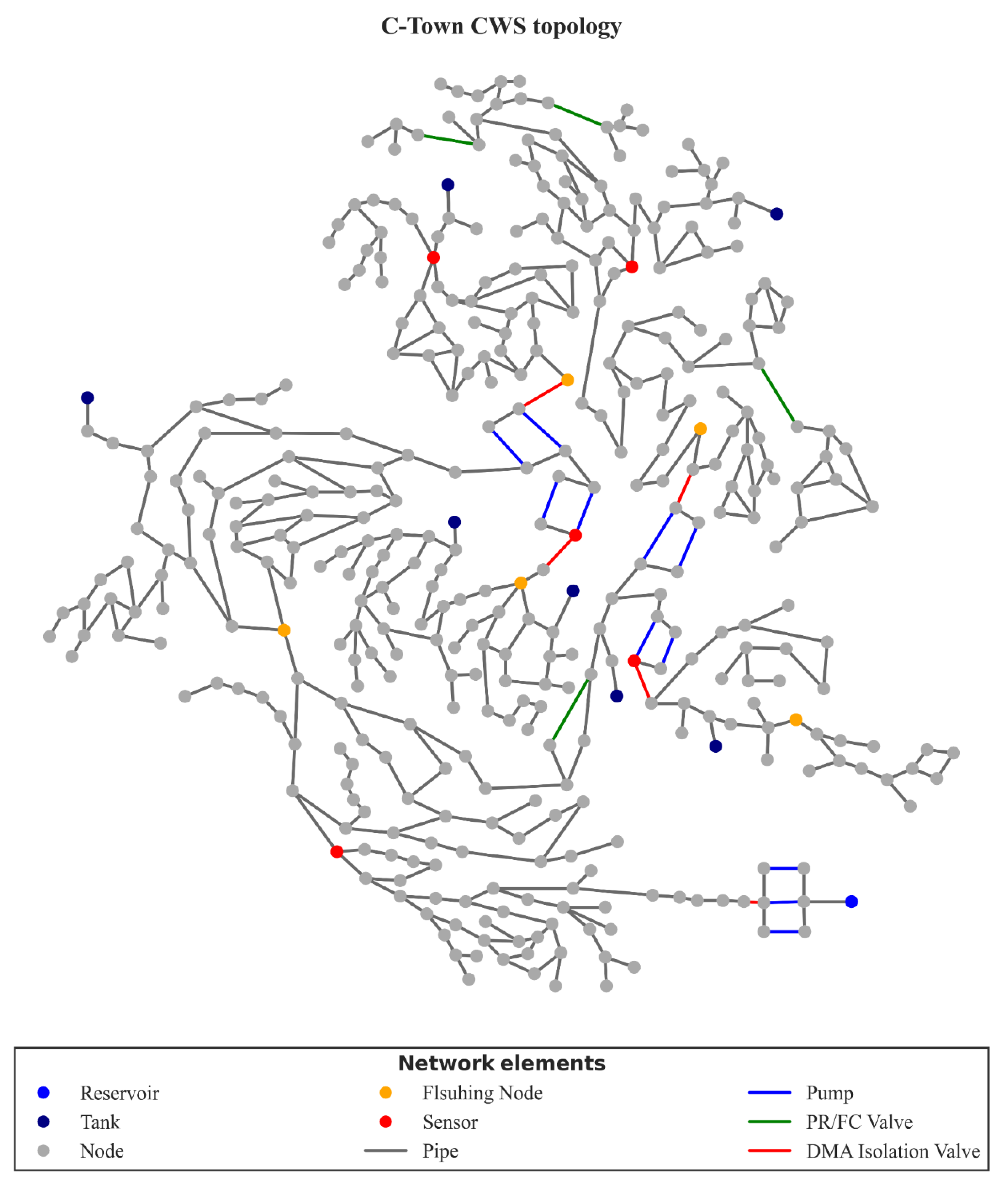
The resilience assessment methodology for CWS under cyber-physical attacks was demonstrated at the C-Town WDN, a benchmark model based on a real medium-sized system used for various studies, e.g., [17,60,61,62]. We used RISKNOUGHT to create a SCADA for the hydraulic controls, as shown in [19], then updated the cyber and physical layers to include a CWS with:

• Four actuators and respective isolation valves that can separate the network into DMAs 1 to 5, placed at pipes P409, P424, P310, P796, and P237;
• Five flushing units (one in each DMA in lower elevation nodes) as new nodes adjacent to present nodes J1056, J416, J1208, J185, and J87 and the necessary actuators and isolation valves for operation; and
• A variable number of water quality sensors depending on sensor design.

Figure 2 shows an example of CWS with these properties. The cyber-physical simulation had duration of 86,400 $\mathrm{s}$, a hydraulic simulation timestep of 600 $\mathrm{s}$, and a water quality timestep of 300 $\mathrm{s}$. The SCADA simulation timestep (how often sensors update and control logic is checked and applied) was matched to the hydraulic step. For the pressure driven demand analysis equations we used for all nodes a minimum pressure of 0 $\mathrm{m}$ and a required pressure of 20 $\mathrm{m}$. The pressure exponent was equal to 0.5.

The controls added for response and mitigation measures depended on the placement of the sensors and had the following form:

• If any sensor detects contamination, isolate all DMAs; and
• If a sensor placed within a DMA detects contamination, activate the corresponding flushing unit and the flushing units in the DMAs that are within the possible path of the contamination extent. For example, if contamination is detected in a node in DMA5, activate the flushing units in DMA5 and DMA1 (from where the water originates).

3.2. Sensor Designs

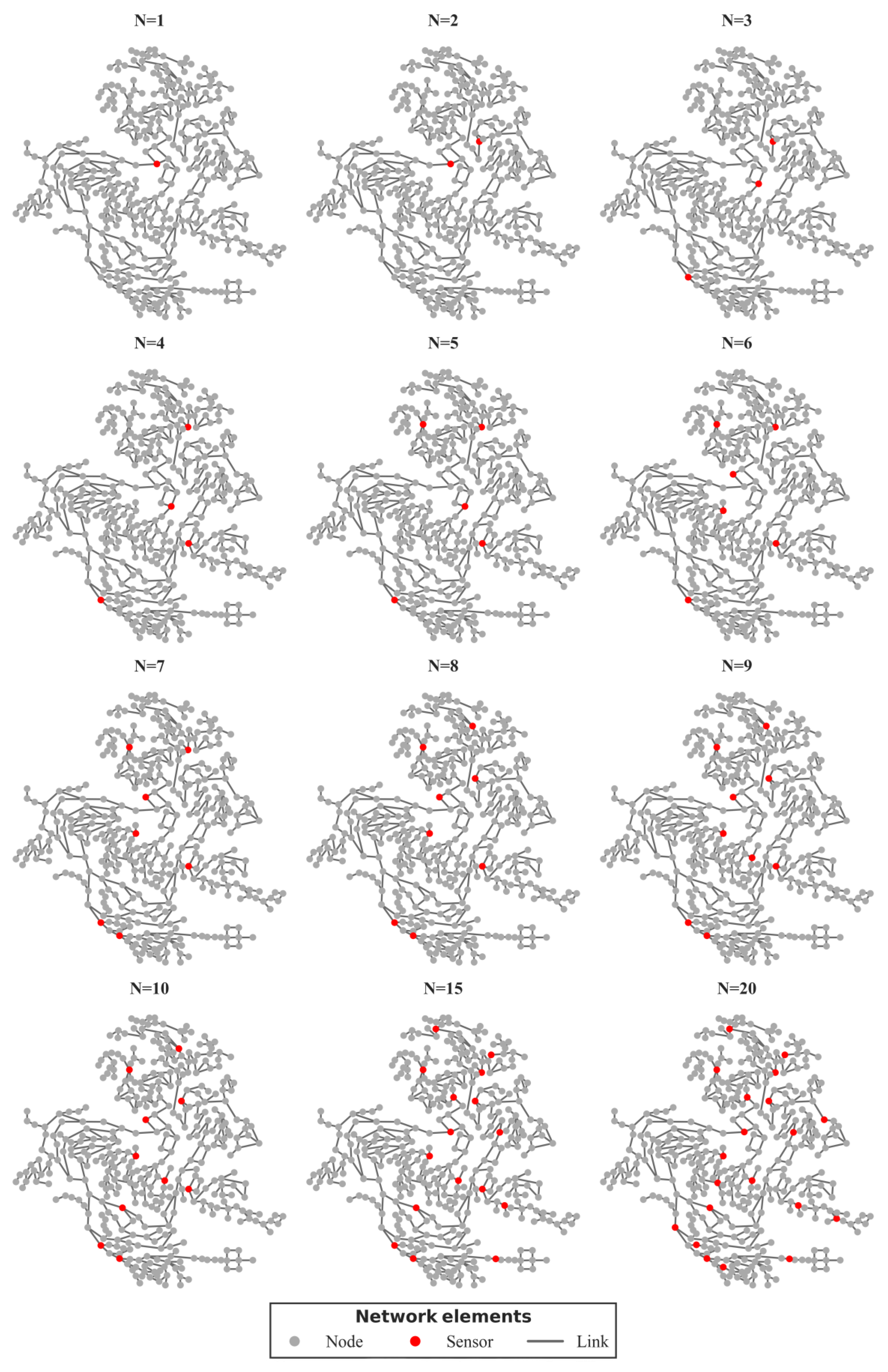
As the associated set of controls included the isolation of DMAs to minimize the spread of contamination, the rational choice of objective function in placement optimization in TEVA-SPOT was minimization of the mean contamination extent. We generated 12 sensor designs of size $N=1, 2,\dots , 10, 15, 20$, as seen in

Table 1. Sensor designs of size $N$ and the sensor ranking of the design.

$\mathbf{Size} \mathit{N}$	Sensor Ranking Order (1st to nth)
$N=1$	J301
$N=2$	J301, J22
$N=3$	J317, J22, J109
$N=4$	J317, J496, J109, J256
$N=5$	J317, J496, J109, J256, J67
$N=6$	J304, J496, J109, J256, J67, J297
$N=7$	J304, J496, J109, J256, J67, J297, J179
$N=8$	J304, J385, J492, J109, J256, J67, J297, J179
$N=9$	J304, J385, J109, J492, J256, J67, J297, J179, J382
$N=10$	J304, J385, J109, J492, J256, J67, J297, J179, J382, J13
$N=15$	J301, J385, J109, J496, J216, J67, J297, J179, J13, J128, J382, J160, J441, J84, J511
$N=20$	J301, J385, J408, J496, J67, J216, J297, J179, J128, J13, J382, J160, J441, J84, J511, J101, J2, J88, J320, J168

with the sensor names and their rankings, by employing 388 (i.e., for all junctions) injection scenarios. The spatial representation is depicted in Figure 3. Designs of size $N = 1 \mathrm{to} 10$ were selected to explore a progressive increase in sensor number, and $N= 15, 20$ to explore designs with a relatively high-monitored locations-to-total nodes ratio (roughly 3.8% and 5.1% respectively).

3.3. Cyber-Physical Scenarios

For the cyber--attack part, the scenarios had progressively more pressure by increasing the number of $k$ most important sensors being manipulated to show normal water quality readings, with $k$ values in the set $\left\{1,2,3,4,5,10,15\right\}$, producing 7 scenario sets. Sensor designs with $N\le k$ were effectively completely unmonitored.

Table 2. Sensors under cyber-attack for each scenario set and sensor design.

$\mathit{N}/\mathit{k}$	$\mathit{k}$= 1	$\mathit{k}$= 2	$\mathit{k}$= 3	$\mathit{k}$= 4	$\mathit{k}$= 5	$\mathit{k}$= 10	$\mathit{k}$= 15
$N$= 1	J301	-	-	-	-	-	-
$N$= 2	J301	J301, J22	-	-	-	-	-
$N$= 3	J317	J317, J22	J317, J22, J109	-	-	-	-
$N$= 4	J317	J317, J496	J317, J496, J109	J317, J496, J109, J256	-	-	-
$N$= 5	J304	J317, J496	J317, J496, J109	J317, J496, J109, J256	J317, J496, J109, J256, J67	-	-
$N$= 6	J304	J317, J496	J304, J496, J109	J304, J496, J109, J256	J304, J496, J109, J256, J67	-	-
$N$= 7	J304	J304, J496	J304, J496, J109	J304, J496, J109, J256	J304, J496, J109, J256, J67	-	-
$N$= 8	J304	J304, J385	J304, J385, J492	J304, J385, J492, J109	J304, J385, J492, J109, J256	-	-
$N$= 9	J304	J304, J385	J304, J385, J109,	J304, J385, J109, J492	J304, J385, J109, J492, J256	-	-
$N$= 10	J304	J304, J385	J304, J385, J109,	J304, J385, J109, J492	J304, J385, J109, J492, J256	J304, J385, J109, J492, J256, J67, J297, J179, J382, J13	-
$N$ = 15	J301	J301, J385	J301, J385, J109,	J301, J385, J109, J492	J301, J385, J109, J492, J216	J301, J385, J109, J492, J216, J67, J297, J179, J13, J128	J301, J385, J109, J492, J216, J67, J297, J179, J13, J128, J382, J160, J441, J84, J511
$N$= 20	J301	J301, J385	J301, J385, J408,	J301, J385, J408, J496	J301, J385, J408, J496, J67	J301, J385, J408, J496, J67, J216, J297, J179, J128, J13	J301, J385, J408, J496, J67, J216, J297, J179, J128, J13, J382, J160, J441, J84, J511

presents the sensors selected by each scenario set from each sensor design $N$.

For the physical attack part, we choose to analyze injections at 15% of the total number of nodes (388), which gave 58 injection locations, sampled with weighted random choice with $l_{lim}=1$ based on the node criticality estimation described above. Figure 4 shows the values of each metric, the nodes’ weighted probabilities, and the final sampled set of injection locations. Each contaminant injection started at time 0 s and ended at time 3600 $\mathrm{s}$ with a mass rate of 1 ${\mathrm{kg} \mathrm{s}}^{-1}$ of a completely conservative contaminant (zero diffusivity and no reactions with water or pipe materials).

4. Results from Stress Testing

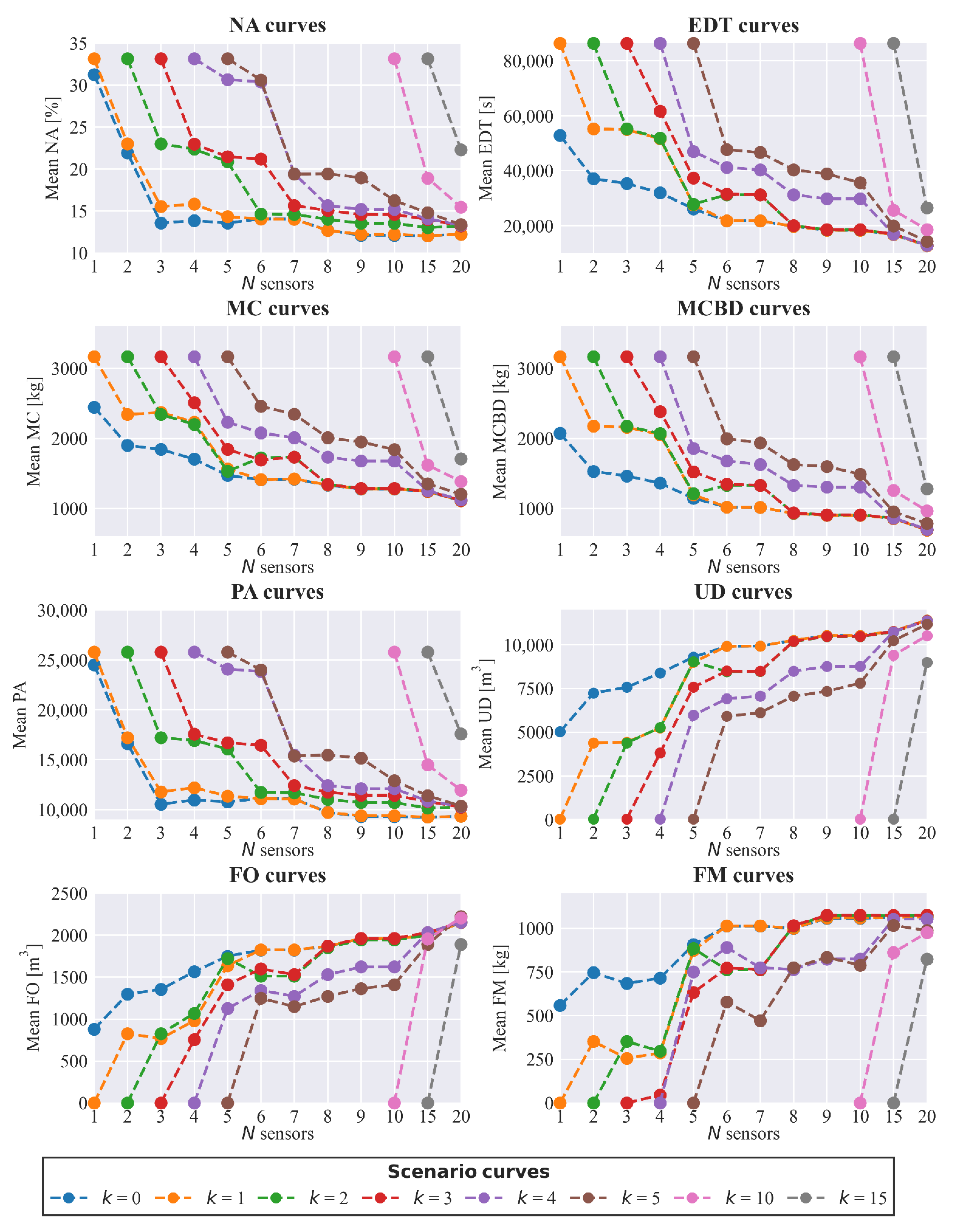
The 58 physical attacks were applied to 12 sensor designs with 7 scenarios of cyber-attacks, as described in Table 2, and also accounting for baseline normal operation of the system, and produced a total of 2900 cyber-physical simulations within a total computational budget of roughly 24 h. Figure 5 shows metric curves that aggregate the results with descriptive metrics. Each curve refers to a scenario set with $k$ attacked sensors with points of the curve describing the mean impact of the scenario set (y-axis) to the topology of $N$ sensors (x-axis).

4.1. Normal Operation

As expected, sensor topologies with more deployed sensors fared better in every metric when no cyber-attack hindered the operation of the CWS, as communicated by the blue curves in the subplots of Figure 5. There were some irregularities, such as, for example, in the $NA$ and $PA$ metrics where the topology of $N=4$ performed slightly worse than the $N=3$ (also true for $N=5$ and $N=6$), but this should be attributed to the small random set of physical attack locations. Had the contaminant injection set included all the possible nodes, the actual performance would have been at least equal. For most of the metrics, performance gains dropped rapidly from $N=8$ onwards, whereas $N=6$ can be regarded as a good trade-off of performance versus deployment cost. Designs with substantially more sensors ($N=15$, $N=20$) generally did not offer much improvement in normal operation status, except for the $EDT$ metric. This exception should be expected, as more sensors equal better coverage and faster detection, but metrics such as $MC$ and $NA$ are affected by the mitigation and response measures, which in this case were the exact same for all sensor designs (i.e., isolation of the five DMAs and activation of the flushing units in the contaminated DMAs). It should be noted that for DMAs where contamination was not detected, no flushing took place. In reality, if contamination is detected usually the water utility issues a public do-not-use warning, and that is why we also employed the $MCBD$ metric. In addition, $FM$ plus $MC$ quantities in scenarios generally do not equal the total injected mass (the same is true for cyber-physical attack scenarios as well), as there are instances where a contaminant mass resides in pipes by the end of the simulation and is neither flushed nor consumed, due to pressure deficient conditions.

4.2. Cyber-Attack Impact

4.2.1. The Case of a Single Attack on the Most Important Sensor

For a small number of deployed sensors ($N\le 5$), the loss of the most important sensor (curve $k=1$) greatly affected most performance metrics because if detection of the contamination were achieved, it would be at a much later stage, as communicated by the $EDT$ metric, which was inflated by the fact that undetected events received the $ed{t}_i$ value of simulation duration. The large increase in impact was not true for $NA$ and $PA$ metrics, where the performance drop was smaller, because these were spatial metrics without a temporal dimension, and for small $N$ values the contamination had a greater spread regardless. For $N>5$ generally the impact was greatly reduced or barely noticeable. This happened because, as seen in Table 1 and Figure 3, the sensor placement optimization algorithm for $N\ge 5$ deployed in all cases sensors that could cover in a redundant way DMA1 (even if not deployed inside, the sensors were close to it), which was the biggest, and it happened that in all sensor designs the most important sensor in ranking was either deployed in J301, J304, or J317, locations on the outskirts of DMA1. This algorithmically unintentional fact gives an insight into the importance of redundancy as a property of resilient design of CWSs.

4.2.2. Effects as $k$ Increased for Designs up to 10 Sensors

Generally, as the strain of the scenarios increased, performance dropped rapidly for most sensor designs. There were a few irregularities for some metrics and curves, such as, for example, mean $MC$ being slightly higher for $k=2$ than $k=3$ for the topology $N=6$, but these can be attributed to the small sample size and some hydraulic conditions that did not alter linearly due to the set of controls for response measures. For metrics $MC$, $MCBD$, and $EDT$, performance was retained for up to $k=3$attacked sensors for sensor designs with $N\ge 8$. Interestingly, the expected $EDT$, $MC$, and $MCBD$ of $N=8, 9, 10$ designs even with the three first ranked sensors taken out were still lower than the $N=5, 6,7$ designs under normal operation conditions, even though the expected spatial extents $NA$ of the contamination events were higher. High performance of these designs up to $k=3$ regarding the $UD$, $FO$, and $FM$ metrics (i.e., high unmet demand, high volume of flushed water, and high mass of flushed contaminant, respectively) signifies that the response and mitigation measures worked as they should, managing to isolate DMAs and flush significant contaminant mass out of the system before being consumed. Therefore, these sensor designs were robust, but when $k>3$, performance rapidly dropped, which was not a desired trait for the CWS, as for resilient designs, failure should be more gradual, i.e., a design that is more safe-to-fail.

4.2.3. Effects as $k$ Increased for Designs with 15 and 20 Sensors

The sensor designs with $N=15$ and $N=20$ proved to be both more robust and more resilient, as demonstrated by their performance. Although it is expected that topologies with significantly more sensors (i.e., at least 50% and 100% more compared to $N\le 10$ designs) outperform the rest, these designs possess an inherent trait of more gradual performance loss. As demonstrated by the $k=10$ curves in Figure 5, even with one quarter and half of the sensors attacked respectively, the performance drop in all metrics was much smaller than the counterparts in other sensor designs. Notably, even with only a quarter of the deployed sensors still operating, $N=20$ design still performed comparably to the un-attacked $N=5$ design in terms of UD $FO$ and $FM$ metrics, showing that the mitigation measures can still provide significant protection fast enough, as communicated by the expected $EDT$ value, even though the contamination spread more $(NA$), affecting more people ($PA$), and contaminant mass consumption was higher before detection ($MCBD$).

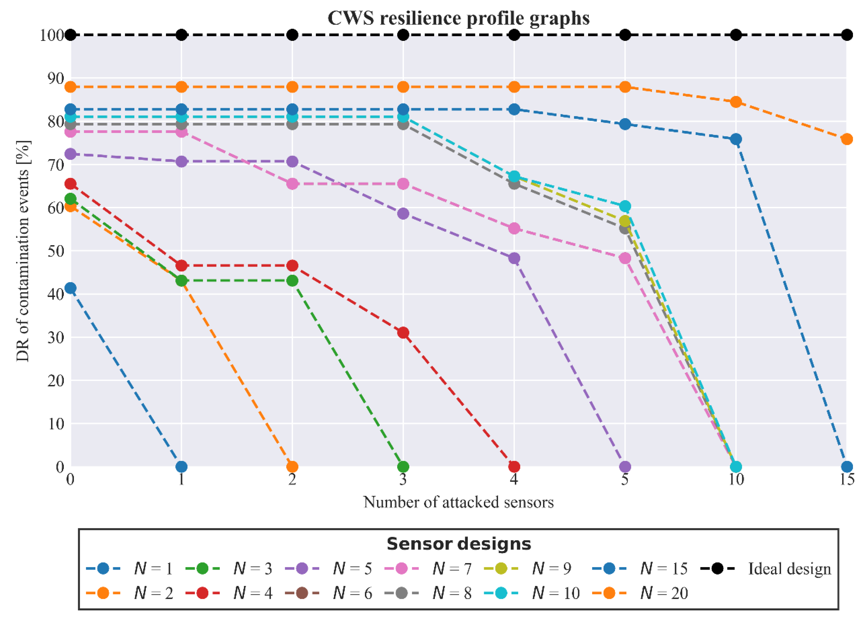
4.3. Resilience Profile Graphs

Examining the metrics presented in Figure 5 allows us to fully describe the system’s behavior under cyber-physical attacks and thus under failure in a variety of scenarios. In addition, we need a well-defined, straightforward, and comprehensible way to measure the reliability of the system to generate resilience profile graphs. Thus, we used the detection rate of the contamination events metric, $DR$, as a surrogate for reliability. The resilience profile graphs for each sensor design are presented in Figure 6. It is evident that sensor designs $N=20$ and $N=15$ were the most resilient and robust. Notably, the resilience score for $N=20$ and this particular ordinal set of disturbances was 85.99%, signifying that even under failure it retains most of its ability to detect contamination in most cases, even when this means lower performance in most other metrics. On the contrary, the $N=6$ sensor design, which seems the best trade-off between performance and cost in normal operation, under these disturbances (some of which, i.e., $k=10, 15$ were well beyond its design capacity) had a much lower resilience score of 48.70%. Even scaled within its design capacity for up to $k=5$, the resilience score was 64.90% owing to its much lower normal operation reliability and greater susceptibility due to the lower count of sensors. In addition, seeming like a paradox, pairs $\left(N=20, k=15\right)$ and $\left(N=20, k=10\right)$attained better reliability (detection rate) than $\left(N=5, k=0\right)$ and $\left(N=10, k=0\right)$, but the actual design goal was to place sensors to minimize the mean extent of contamination, and this was a surprising side-effect. The remaining working sensors in $N=20$ happened to fare in detection rates better than the complete sets of sensors in $N=5$and $N=10$, as these were be placed in less central locations (due to their lower ranking) and thus, monitor more locations, increasing network coverage. It should also be noted that designs $N=6$ and $N=7$ had exactly the same resilience results. This was to be expected, as these designs had the same sensors, except the lowest ranked sensor in $N=7$ (placed at J179), which was placed at a position monitoring locations that were a subset of locations monitored by the sixth sensor (placed at J297) in both designs. The resilience scores are presented in

Table 3. Resilience scores for the examined sensor designs and scenarios, as measured by comparing the area under the reliability curve with the area of the ideal CWS design.

Design	Resilience Score
$N=1$	2.96%
$N=2$	10.47%
$N=3$	16.74%
$N=4$	22.41%
$N=5$	40.46%
$N=6$	50.12%
$N=7$	50.12%
$N=8$	56.90%
$N=9$	58.25%
$N=10$	58.74%
$N=15$	75.37%
$N=20$	86.57%

.

5. Comparing Resilience of Different Sensor Deployment Strategies

5.1. Generating Topologies with Other Placement Optimization Strategies

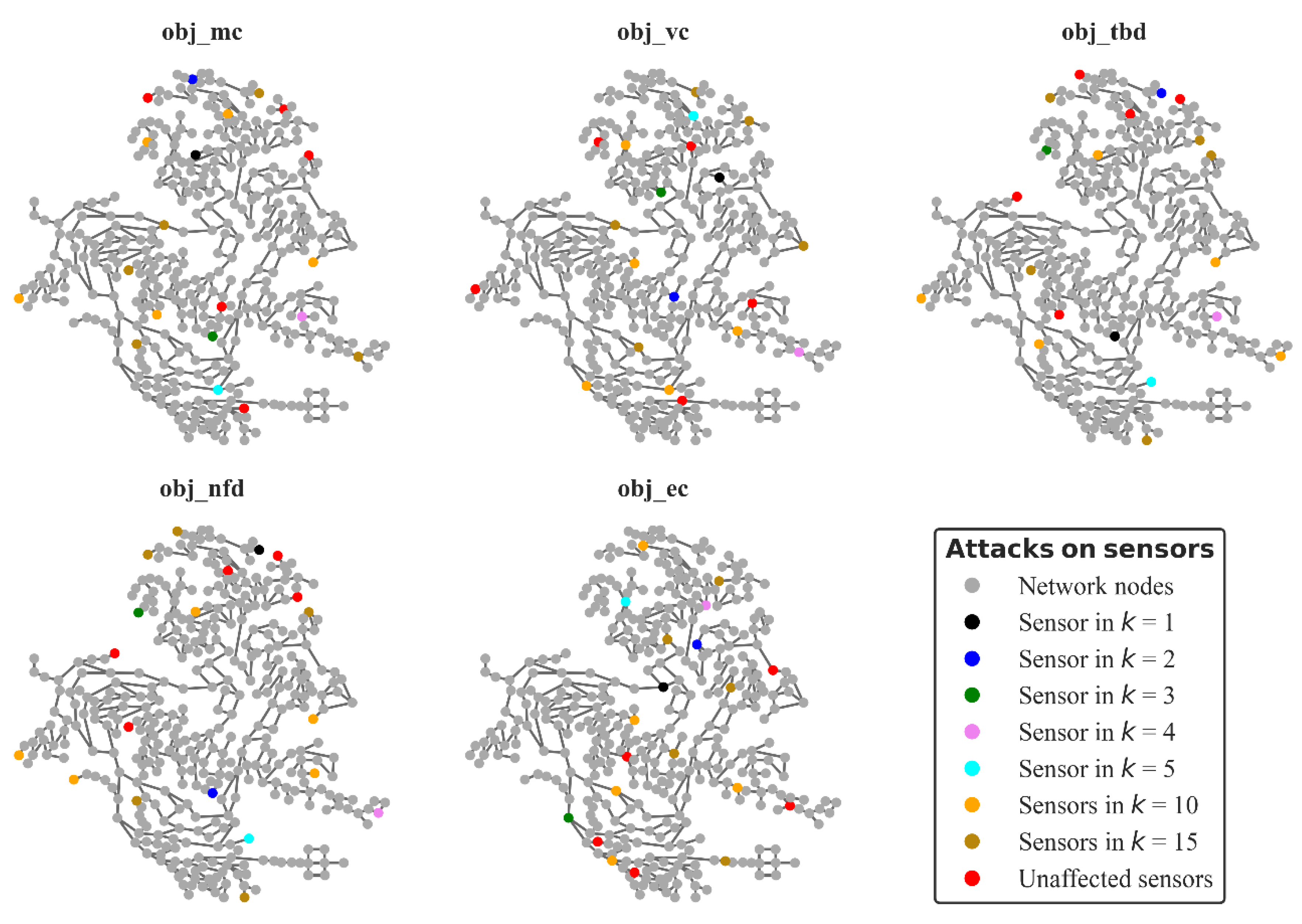
The behavior of the $N=20$ topology generated by optimizing the placement with the objective function mean contamination extent ($obj\_ec$) exhibited, as expected, better performance than other topologies with a lower number of sensors, but also showed robustness and resilience traits. This brings up the question of whether using other topologies comparable in the number of sensors would fortify the network with better performance under loss of function due to cyber-physical attacks. Using TEVA-SPOT, four more topologies of 20 sensors were generated using the objective functions (i) minimize mean mass consumed, $obj\_mc$, (ii) minimize mean volume consumed, $obj\_vc$, (iii) minimize mean time before detection, $obj\_tbd$, and (iv) minimize mean number of failed detections, $obj\_nfd$. The sensors selected for each objective function are shown in

Table 4. Sensors generated from other objective functions, arranged by rank from most to least critical.

$\mathit{o}\mathit{b}\mathit{j}\_\mathit{m}\mathit{c}$	$\mathit{o}\mathit{b}\mathit{j}\_\mathit{v}\mathit{c}$	$\mathit{o}\mathit{b}\mathit{j}\_\mathit{t}\mathit{b}\mathit{d}$	$\mathit{o}\mathit{b}\mathit{j}\_\mathit{n}\mathit{f}\mathit{d}$
J237, J574, J360, J344, J7, J61, J487, J81, J379, J305, J157, J201, J296, J439, J224, J232, J150, J27, J499, J165	J257, J382, J86, J94, J492, J7, J297, J67, J109, J216, J32, J201, J414, J169, J509, J226, J192, J1170, J576, J61	J360, J224, J69, J345, J1058, J81, J379, J123, J237, J439, J296, J167, J284, J150, J27, J153, J487, J504, J305, J334	J224, J360, J70, J123, J1058, J81, J345, J379, J237, J144, J167, J439, J150, J153, J27, J284, J296, J334, J487, J504

. The same selecting methodology of $k$ best ranked sensors for cyber-attacks and the same injection location set were used to compare performance. For better comparison purposes we used all $k$ sets for $k\in \left\{0,15\right\}$. Figure 7 depicts the sensors’ locations in the network, color coded by sets of attacks.

5.2. CWS Resilience Results of Various Sensor Placement Strategies

By subjecting the topologies of 20 sensors generated by the $obj\_mc$, $obj\_vc$, $obj\_tbd$, and $obj\_nfd$ to the same stress-testing procedure as the $N=20$ topology of the $obj\_ec$, we acquired the results presented in Figure 8. As expected, the topology of the design strategy of minimizing the mean detection failure ($obj\_nfd$) yielded the best reliability score for undisrupted service, near the ideal design at 98.27%. In this state, performance (it should be noted that by performance hereafter we refer to detection rate—not the performance of any other metric) was matched by strategy $obj\_tbd$, which employed a very similar sensor set but with different rankings for the exact same sensors ($obj\_tbd$ was better in $k=7$ but worse in $k=2,11,12,13$), then followed closely by $obj\_mc$ with 96.55%, $obj\_vc$ exhibiting a high score of 93.10%, and the lowest performance attributed to $obj\_ec$ at 87.93%. Interestingly, as the disruption to the system increased with progressively attacking the $k$ most important sensors, the reliability in detecting contaminations of $obj\_nfd$ and $obj\_tbd$ diminished to 70.68% (a performance delta of 27.59%), taking the last place, whereas $obj\_ec$ rose to first place with 75.86% (a smaller performance delta of 12.07%). The two other strategies shared the second rank, where $obj\_mc$and $obj\_vc$ demonstrated performance deltas of 22.41% and 18.97%, respectively. The performance curves exhibited different characteristics: $obj\_tbd$ lost reliability immediately at $k=1$, $obj\_nfd$ and $obj\_vc$ started to lose reliability at $k=2$, and $obj\_mc$ weathered the disturbance up to $k=3$. The robustness trait of $obj\_ec$ to withstand up to $k=8$ is remarkable given that while it was not the top performing strategy by design in reliability to detect contamination, by $k=6$ it had closed the performance gap with the other strategies and then outperformed them all at every $k>9$. Looking at the resilience scores, we got the following scores: $obj\_ec$ was the most resilient with a score of 85.23%, then followed $obj\_mc$ with 84.54%, $obj\_vc$ with 83.85%, and both $obj\_nfd$ and $obj\_tbd$ sharing the last position with 83.22%.

6. Insights from the Case Study for CWS Design

This study is the first to the authors’ knowledge in which the resilience of different sensor designs is assessed under complex cyber-physical attacks, including deliberate contamination, where the cyber-physical model employs a series of realistic response and mitigation measures in an integrated control scheme that affects the actual outcome of the simulation, measured with multidimensional measures. The results obtained by this case are transferable to real-world water distribution networks, and signify the interplay between different attributes of sensor designs, such as increased sensor count, redundancy in monitored locations, and control actions. As shown, small variations in sensor size design can have anywhere from unnoticeable to big impacts on performance in metrics when under loss of operation of some elements, with some designs unintentionally proving to be more resilient or robust. It is self-explanatory that more sensors equal better performance, but even one more sensor placed at a carefully chosen location can provide a great benefit against loss of function and redundancy in the network. Moreover, the examination of the behavior of different sensor designs against the same sets of attacks shows that there are cases where a generally less optimal solution in detecting contamination for normal operation status (e.g., $obj\_ec$ versus $obj\_nfd$) is eventually far more robust and resilient against disturbance, perhaps counterintuitively. This insight is also shared with many other engineered systems: A top-performing and reliable system at normal operation status is not always resilient, as there are also robust systems that are not resilient [43,63]. This behavior can only be evaluated by systematic stress-testing procedures that assess the performance of the system under failure, denoting the importance of such resilient assessment methodologies for engineered systems.

Because in this study the cyber-attacks are deliberately chosen from sensor ranking order, the fact that some designs can be more resilient can only be exacerbated by more targeted attacks that can, for example, blind sensors monitoring the same DMA regardless of ranking. As such, we conclude that sensor placement optimization methodologies should generally take into account the possibility of a subset of sensors not operating. In addition, by carefully examining the sensor placement locations of the various strategies employed, it is evident that the strategies $obj\_nfd$ and $obj\_tbd$ deploy all sensors to the outskirts of the network at terminal nodes, $obj\_mc$ places 40% of them, and on the contrary $obj\_vc$ and $obj\_ec$ none of them. This fact suggests that there is some connection with the choice of placement locations and inherent resilience against disturbances in the capacity to eventually detect contamination due to loss of performance because of deliberate attacks and could be exploited to design algorithms to place sensors with the goal of optimizing CWS resilience. Moreover, the resilience assessment methodology presented here is generally applicable to case studies with simple malfunctions or inability of sensors to detect contamination that may also not be deliberate, but accidental, and thus can be employed outside of cyber-physical design studies without modification.

Although we study the problem from a “what-if” civil engineering perspective, there are two more aspects of the resilience assessment performed here that can be improved upon through interdisciplinary research efforts. The first is the fact that both the contaminant and the sensors are deprived from their chemical nature to simplify things. Obviously, contaminants rarely are as persistent and conservative as in the simulations here and react with water, pipe materials, etc., possibly forming even more dangerous substances. Sensors typically monitor surrogate quality properties of water to detect anomalies, and thus may not always detect a contaminant. A multi-species water quality analysis with an analysis of the reactions and kinetics of the contaminant and the impact on sensor monitor properties can give a more accurate representation of the cyber-physical control scheme and impact assessment of the cyber-physical attack. The second is the IT (information technology) aspect of the cyber-physical system. Although no cyber system is unsusceptible to hacking, there can be solutions implemented that hinder certain types of attacks, or some elements of the system that can be of different technology, and such measures should be addressed in a more realistic representation of the problem and its scenario simulation.

7. Conclusions

We presented a formal resilience assessment methodology for different water quality sensor designs in cyber-physical water distribution systems under cyber-physical threats. We also demonstrated the use of the methodology through a comprehensive analysis of a medium-sized real-world-based WDN under a multitude of cyber-attacks combined with a wide range of deliberate physical contamination attacks and evaluated its performance with multidimensional metrics. The results show that resilience and robustness are traits of the system that can be assessed only by stress-testing methodologies that evaluate the system’s performance under failure. It is suggested that this methodology can prove useful to water utility risk assessment, risk mitigation studies, and strategic planning, as well as inform water quality sensor placement decisions.

References

- Yang, X.; Boccelli, D.L. Model-Based Event Detection for Contaminant Warning Systems. J. Water Resour. Plan. Manag. 2016, 142, 04016048. [Google Scholar] [CrossRef]
- Clark, R.M.; Deininger, R.A. Protecting the Nation’s Critical Infrastructure: The Vulnerability of U.S. Water Supply Systems. J. Contingencies Cris. Manag. 2000, 8, 73–80. [Google Scholar] [CrossRef]
- Mac Kenzie, W.R.; Hoxie, N.J.; Proctor, M.E.; Gradus, M.S.; Blair, K.A.; Peterson, D.E.; Kazmierczak, J.J.; Addiss, D.G.; Fox, K.R.; Rose, J.B.; et al. A Massive Outbreak in Milwaukee of Cryptosporidium Infection Transmitted through the Public Water Supply. N. Engl. J. Med. 1994, 331, 161–167. [Google Scholar] [CrossRef]
- Hoxie, N.J.; Davis, J.P.; Vergeront, J.M.; Nashold, R.D.; Blair, K.A. Cryptosporidiosis-associated mortality following a massive waterborne outbreak in Milwaukee, Wisconsin. Am. J. Public Health 1997, 87, 2032–2035. [Google Scholar] [CrossRef] [Green Version]
- Corso, P.S.; Kramer, M.H.; Blair, K.A.; Addiss, D.G.; Davis, J.P.; Haddix, A.C. Cost of illness in the 1993 waterborne Cryptosporidium outbreak, Milwaukee, Wisconsin. Emerg. Infect. Dis. 2003, 9, 426–431. [Google Scholar] [CrossRef] [PubMed]
- Thomasson, E.D.; Scharman, E.; Fechter-Leggett, E.; Bixler, D.; Ibrahim, S.; Duncan, M.A.; Hsu, J.; Scott, M.; Wilson, S.; Haddy, L.; et al. Acute Health Effects After the Elk River Chemical Spill, West Virginia, January 2014. Public Health Rep. 2017, 132, 196–202. [Google Scholar] [CrossRef] [Green Version]
- Zheng, F.; Du, J.; Diao, K.; Zhang, T.; Yu, T.; Shao, Y. Investigating Effectiveness of Sensor Placement Strategies in Contamination Detection within Water Distribution Systems. J. Water Resour. Plan. Manag. 2018, 144, 06018003. [Google Scholar] [CrossRef]
- Qiu, M.; Salomons, E.; Ostfeld, A. A framework for real-time disinfection plan assembling for a contamination event in water distribution systems. Water Res. 2020, 174, 115625. [Google Scholar] [CrossRef]
- Nilsson, K.A.; Buchberger, S.G.; Clark, R.M. Simulating exposures to deliberate intrusions into water distribution systems. J. Water Resour. Plan. Manag. 2005, 131, 228–236. [Google Scholar] [CrossRef]
- Gleick, P.H. Water and terrorism. Water Policy 2006, 8, 481–503. [Google Scholar] [CrossRef] [Green Version]
- Rasekh, A.; Brumbelow, K. A dynamic simulation-optimization model for adaptive management of urban water distribution system contamination threats. Appl. Soft Comput. J. 2015, 32, 59–71. [Google Scholar] [CrossRef] [Green Version]
- Ginsberg, M.D.; Hock, V.F. Terrorism and security of water distribution systems: A primer. Def. Secur. Anal. 2004, 20, 373–380. [Google Scholar] [CrossRef]
- Danneels, J.J.; Finley, R.E. Assessing the Vulnerabilities of U.S. Drinking Water Systems. J. Contemp. Water Res. Educ. 2009, 129, 8–12. [Google Scholar] [CrossRef]
- Maiolo, M.; Pantusa, D. Infrastructure Vulnerability Index of drinking water systems to terrorist attacks. Cogent Eng. 2018, 5. [Google Scholar] [CrossRef]
- Pelekanos, N.; Nikolopoulos, D.; Makropoulos, C. Simulation and vulnerability assessment of water distribution networks under deliberate contamination attacks. Urban Water J. 2021, 1–14. [Google Scholar] [CrossRef]
- Manzi, D.; Giacomoni, M.; Izquierdo, J.; Ostfeld, A.; Brentan, B.M.; Pourahmadi, M.; Gatsis, N.; Pasha, M.F.K.; Lo, C.S.; Ohar, Z.; et al. Battle of the Attack Detection Algorithms: Disclosing Cyber Attacks on Water Distribution Networks. J. Water Resour. Plan. Manag. 2018, 144, 04018048. [Google Scholar] [CrossRef] [Green Version]
- Taormina, R.; Galelli, S.; Tippenhauer, N.O.; Salomons, E.; Ostfeld, A. Characterizing Cyber-Physical Attacks on Water Distribution Systems. J. Water Resour. Plan. Manag. 2017, 143, 04017009. [Google Scholar] [CrossRef]
- Taormina, R.; Galelli, S.; Tippenhauer, N.O.; Salomons, E.; Ostfeld, A. Simulation of cyber-physical attacks on water distribution systems with EPANET. Cryptol. Inf. Secur. Ser. 2016, 14, 123–130. [Google Scholar] [CrossRef]
- Nikolopoulos, D.; Moraitis, G.; Bouziotas, D.; Lykou, A.; Karavokiros, G.; Makropoulos, C. Cyber-Physical Stress-Testing Platform for Water Distribution Networks. J. Environ. Eng. 2020, 146, 04020061. [Google Scholar] [CrossRef]
- Nikolopoulos, D.; Makropoulos, C.; Kalogeras, D.; Monokrousou, K.; Tsoukalas, I. Developing a Stress-Testing Platform for Cyber-Physical Water Infrastructure. In Proceedings of the 2018 International Workshop on Cyber-physical Systems for Smart Water Networks (CySWater), Cincinnati, OH, USA, 10–13 April 2018; IEEE: Porto, Portugal, 2018; pp. 9–11. [Google Scholar]
- Almalawi, A.; Tari, Z.; Khalil, I.; Fahad, A. SCADAVT-A framework for SCADA security testbed based on virtualization technology. In Proceedings of the 38th Annual IEEE Conference on Local Computer Networks, Sydney, Australia, 21–24 October 2013; IEEE: Sydney, Australia, 2013; pp. 639–646. [Google Scholar]
- Lee, E. The Past, Present and Future of Cyber-Physical Systems: A Focus on Models. Sensors 2015, 15, 4837–4869. [Google Scholar] [CrossRef] [PubMed]
- Alfonso, L.; Jonoski, A.; Solomatine, D. Multiobjective optimization of operational responses for contaminant flushing in water distribution networks. J. Water Resour. Plan. Manag. 2010, 136, 48–58. [Google Scholar] [CrossRef]
- Hart, W.E.; Murray, R. Review of Sensor Placement Strategies for Contamination Warning Systems in Drinking Water Distribution Systems. J. Water Resour. Plan. Manag. 2010, 136, 611–619. [Google Scholar] [CrossRef]
- Ostfeld, A.; Salomons, E. Optimal Layout of Early Warning Detection Stations for Water Distribution Systems Security. J. Water Resour. Plan. Manag. 2004, 130, 377–385. [Google Scholar] [CrossRef]
- Yaroshenko, I.; Kirsanov, D.; Marjanovic, M.; Lieberzeit, P.A.; Korostynska, O.; Mason, A.; Frau, I.; Legin, A. Real-Time Water Quality Monitoring with Chemical Sensors. Sensors 2020, 20, 3432. [Google Scholar] [CrossRef] [PubMed]
- Kavi Priya, S.; Shenbagalakshmi, G.; Revathi, T. Design of smart sensors for real time drinking water quality monitoring and contamination detection in water distributed mains. Int. J. Eng. Technol. 2017, 7, 47. [Google Scholar] [CrossRef] [Green Version]
- Ostfeld, A.; Salomons, E. Optimal early warning monitoring system layout for water networks security: Inclusion of sensors sensitivities and response delays. Civ. Eng. Environ. Syst. 2005, 22, 151–169. [Google Scholar] [CrossRef]
- Kessler, A.; Ostfeld, A.; Sinai, G. Detecting Accidental Contaminations in Municipal Water Networks. J. Water Resour. Plan. Manag. 1998, 124, 192–198. [Google Scholar] [CrossRef]
- Weickgenannt, M.; Kapelan, Z.; Blokker, M.; Savic, D.A. Risk-Based Sensor Placement for Contaminant Detection in Water Distribution Systems. J. Water Resour. Plan. Manag. 2010, 136, 629–636. [Google Scholar] [CrossRef]
- Zhang, Q.; Zheng, F.; Kapelan, Z.; Savic, D.; He, G.; Ma, Y. Assessing the global resilience of water quality sensor placement strategies within water distribution systems. Water Res. 2020, 172, 115527. [Google Scholar] [CrossRef] [PubMed]
- Rathi, S.; Gupta, R. A simple sensor placement approach for regular monitoring and contamination detection in water distribution networks. KSCE J. Civ. Eng. 2016, 20, 597–608. [Google Scholar] [CrossRef]
- Krause, A.; Leskovec, J.; Guestrin, C.; VanBriesen, J.; Faloutsos, C. Efficient Sensor Placement Optimization for Securing Large Water Distribution Networks. J. Water Resour. Plan. Manag. 2008, 134, 516–526. [Google Scholar] [CrossRef] [Green Version]
- Berry, J.; Hart, W.E.; Phillips, C.A.; Uber, J.G.; Watson, J.-P. Sensor Placement in Municipal Water Networks with Temporal Integer Programming Models. J. Water Resour. Plan. Manag. 2006, 132, 218–224. [Google Scholar] [CrossRef] [Green Version]
- Klise, K.A.; Bynum, M.; Moriarty, D.; Murray, R. A software framework for assessing the resilience of drinking water systems to disasters with an example earthquake case study. Environ. Model. Softw. 2017, 95, 420–431. [Google Scholar] [CrossRef]
- Propato, M. Contamination Warning in Water Networks: General Mixed-Integer Linear Models for Sensor Location Design. J. Water Resour. Plan. Manag. 2006, 132, 225–233. [Google Scholar] [CrossRef]
- Lee, B.H.; Deininger, R.A. Optimal Locations of Monitoring Stations in Water Distribution System. J. Environ. Eng. 1992, 118, 4–16. [Google Scholar] [CrossRef]
- Berry, J.; Carr, R.D.; Hart, W.E.; Leung, V.J.; Phillips, C.A.; Watson, J.-P. Designing Contamination Warning Systems for Municipal Water Networks Using Imperfect Sensors. J. Water Resour. Plan. Manag. 2009, 135, 253–263. [Google Scholar] [CrossRef]
- Preis, A.; Ostfeld, A. Genetic algorithm for contaminant source characterization using imperfect sensors. Civ. Eng. Environ. Syst. 2008, 25, 29–39. [Google Scholar] [CrossRef]
- Nikolopoulos, D.; van Alphen, H.-J.; Vries, D.; Palmen, L.; Koop, S.; van Thienen, P.; Medema, G.; Makropoulos, C. Tackling the “New Normal”: A Resilience Assessment Method Applied to Real-World Urban Water Systems. Water 2019, 11, 330. [Google Scholar] [CrossRef] [Green Version]
- Makropoulos; Savić Urban Hydroinformatics: Past, Present and Future. Water 2019, 11, 1959. [CrossRef] [Green Version]
- Nikolopoulos, D.; Makropoulos, C. Cyber-Physical Quality Attack Modelling and Stress-Testing for Water Distribution Networks. Urban Water J. 2020, 146, 04020061. [Google Scholar]
- Makropoulos, C.; Nikolopoulos, D.; Palmen, L.; Kools, S.; Segrave, A.; Vries, D.; Koop, S.; van Alphen, H.J.; Vonk, E.; van Thienen, P.; et al. A resilience assessment method for urban water systems. Urban Water J. 2018, 15, 316–328. [Google Scholar] [CrossRef]
- Holling, C.S. Resilience and Stability of Ecological Systems. Annu. Rev. Ecol. Syst. 1973, 4, 1–23. [Google Scholar] [CrossRef] [Green Version]
- Mugume, S.N.; Gomez, D.E.; Fu, G.; Farmani, R.; Butler, D. A global analysis approach for investigating structural resilience in urban drainage systems. Water Res. 2015, 81, 15–26. [Google Scholar] [CrossRef] [Green Version]
- Hashimoto, T.; Stedinger, J.R.; Loucks, D.P. Reliability, resiliency, and vulnerability criteria for water resource system performance evaluation. Water Resour. Res. 1982, 18, 14–20. [Google Scholar] [CrossRef] [Green Version]
- Butler, D.; Ward, S.; Sweetapple, C.; Astaraie-Imani, M.; Diao, K.; Farmani, R.; Fu, G. Reliable, resilient and sustainable water management: The Safe & SuRe approach. Glob. Chall. 2017, 1, 63–77. [Google Scholar] [CrossRef]
- Francis, R.; Bekera, B. A metric and frameworks for resilience analysis of engineered and infrastructure systems. Reliab. Eng. Syst. Saf. 2014, 121, 90–103. [Google Scholar] [CrossRef]
- Ciaponi, C.; Creaco, E. Comparison of Pressure-Driven Formulations for WDN Simulation. Water 2018, 10, 523. [Google Scholar] [CrossRef] [Green Version]
- Rossman, L.A.; Woo, H.; Tryby, M.; Shang, F.; Janke, R.; Haxton, T. EPANET 2.2 User Manual; U.S. Environmental Protection Agency: Cincinnati, OH, USA, 2020.
- Berry, J.; Boman, E.; Riesen, L.A.; Hart, W.E.; Phillips, C.A.; Watson, J.-P. User’s Manual: TEVA-SPOT Toolkit 2.5.2; U.S. Environmental Protection Agency: Cincinnati, OH, USA, 2012. [Google Scholar]
- Watson, J.P.; Greenberg, H.J.; Hart, W.E. A multiple-objective analysis of sensor placement optimization in water networks. In Critical Transitions in Water and Environmental Resources Management; American Society of Civil Engineers: Cincinnati, OH, USA, 2004; pp. 4609–4618. [Google Scholar] [CrossRef]
- Ostfeld, A.; Salomons, E. Sensor Network Design Proposal for the Battle of the Water Sensor Networks (BWSN). In Proceedings of the Water Distribution Systems Analysis Symposium, Cincinnati, OH, USA, 27–30 August 2006; American Society of Civil Engineers: Cincinnati, OH, USA, 2006; pp. 1–16. [Google Scholar]
- Ostfeld, A.; Uber, J.G.; Salomons, E.; Berry, J.W.; Hart, W.E.; Phillips, C.A.; Watson, J.-P.; Dorini, G.; Jonkergouw, P.; Kapelan, Z.; et al. The Battle of the Water Sensor Networks (BWSN): A Design Challenge for Engineers and Algorithms. J. Water Resour. Plan. Manag. 2008, 134, 556–568. [Google Scholar] [CrossRef] [Green Version]
- Klise, K.A.; Nicholson, B.; Laird, C.D. Sensor Placement Optimization Using Chama; Sandia National Laboratories: Albuquerque, NM, USA, 2017. [Google Scholar]
- Freeman, L.C. A Set of Measures of Centrality Based on Betweenness. Sociometry 1977, 40, 35. [Google Scholar] [CrossRef]
- Giudicianni, C.; Herrera, M.; Di Nardo, A.; Greco, R.; Creaco, E.; Scala, A. Topological Placement of Quality Sensors in Water-Distribution Networks without the Recourse to Hydraulic Modeling. J. Water Resour. Plan. Manag. 2020, 146, 04020030. [Google Scholar] [CrossRef]
- Santonastaso, G.F.; Di Nardo, A.; Creaco, E.; Musmarra, D.; Greco, R. Comparison of topological, empirical and optimization-based approaches for locating quality detection points in water distribution networks. Environ. Sci. Pollut. Res. 2020. [Google Scholar] [CrossRef]
- Moraitis, G.; Nikolopoulos, D.; Bouziotas, D.; Lykou, A.; Karavokiros, G.; Makropoulos, C. Quantifying Failure for Critical Water Infrastructures under Cyber-Physical Threats. J. Environ. Eng. 2020, 146, 04020108. [Google Scholar] [CrossRef]
- Taormina, R.; Galelli, S. Deep-Learning Approach to the Detection and Localization of Cyber-Physical Attacks on Water Distribution Systems. J. Water Resour. Plan. Manag. 2018, 144, 04018065. [Google Scholar] [CrossRef]
- Nikolopoulos, D.; Moraitis, G.; Bouziotas, D.; Lykou, A.; Karavokiros, G.; Makropoulos, C. RISKNOUGHT: A Cyber-Physical Stress-Testing Platform For Water Distribution Networks. In Proceedings of the 11th World Congress on Water Resources and Environment (EWRA 2019) “Managing Water Resources for a Sustainable Future”, Madrid, Spain, 2–6 July 2019. [Google Scholar]
- Sankary, N.; Ostfeld, A. Bayesian Localization of Water Distribution System Contamination Intrusion Events Using Inline Mobile Sensor Data. J. Water Resour. Plan. Manag. 2019, 145, 04019029. [Google Scholar] [CrossRef]
- Read, D. Some observations on resilience and robustness in human systems. Cybern. Syst. 2005, 36, 773–802. [Google Scholar] [CrossRef] [Green Version]
Figure 1.
CWS resilience profile graphs.
Figure 2.
Example of CWS topology for C-Town with a sensor design of five sensors.
Figure 3.
Sensor topologies generated by TEVA-SPOT for different numbers of sensors ().
Figure 4.
Betweenness centrality, node reach, probability distribution of sampling choice, and the final sampled locations with .
Figure 5.
Metric curves from the results of the simulations.
Figure 6.
CWS resilience profile graphs for reliability metric . It should be noted that and curves are indiscernible.
Figure 7.
Topologies of 20 sensors as placed by the objective functions used in this work, color coded by the set of attacks they belong to (some representative sets are selected).
Figure 8.
Resilience profile graphs for the five objective functions used to generate topologies of 20 sensors.