Numerical Simulations of the Flow Field of a Submerged Hydraulic Jump over Triangular Macroroughnesses

Abstract

The submerged hydraulic jump is a sudden change from the supercritical to subcritical flow, specified by strong turbulence, air entrainment and energy loss. Despite recent studies, hydraulic jump characteristics in smooth and rough beds, the turbulence, the mean velocity and the flow patterns in the cavity region of a submerged hydraulic jump in the rough beds, especially in the case of triangular macroroughnesses, are not completely understood. The objective of this paper was to numerically investigate via the FLOW-3D model the effects of triangular macroroughnesses on the characteristics of submerged jump, including the longitudinal profile of streamlines, flow patterns in the cavity region, horizontal velocity profiles, streamwise velocity distribution, thickness of the inner layer, bed shear stress coefficient, Turbulent Kinetic Energy (TKE) and energy loss, in different macroroughness arrangements and various inlet Froude numbers (1.7 < Fr₁ < 9.3). To verify the accuracy and reliability of the present numerical simulations, literature experimental data were considered.

1. Introduction

Hydraulic jumps with intense turbulent mixing and air bubble entrainment are regarded as a change process from supercritical to subcritical flow [1]. Free and submerged hydraulic jumps are usually suitable for energy loss under hydraulic structures such as gates, spillways and weirs. The characteristics of hydraulic jumps on the smooth bed have been widely studied [2,3,4,5,6,7,8,9]. Several experimental and numerical studies have been performed on the free and submerged hydraulic jumps over macroroughnesses to foresee how the roughness elements of the bed affect the characteristics of hydraulic jumps compared to the smooth bed. Ead and Rajaratnam [10] investigated the properties of hydraulic jump on sinusoidal macroroughnesses and normalized the water surface profile and discharge with non-dimensional analysis. Tokyay et al. [11] observed that the jump length ratio and energy loss over two sinusoidal macroroughnesses were 35% smaller and 6% higher than a smooth bed, respectively. Abbaspour et al. [12] studied the properties of a hydraulic jump over six sinusoidal macroroughnesses. The results stated that the tailwater depth and jump length were lower than the smooth bed and the Froude number had a great impact on the jump length. Shafai-Bejestan and Neisi [13] investigated the effects of lozenge macroroughnesses on the hydraulic jump. The results showed that the use of lozenge macroroughnesses reduced the tailwater depth and jump length compared with the smooth bed. Izadjoo and Shafai-Bejestan [14] studied hydraulic jumps on various trapezoidal macroroughnesses. They observed that the shear stress coefficient was over ten times larger than that on the smooth bed, and the jump length decreased by 50%. Nikmehr and Aminpour [15] investigated the properties of a hydraulic jump over macroroughnesses with trapezoidal blocks using the Flow-3D model Version 11.2 [16]. The results stated that increasing the height and the distance of the macroroughnesses, the velocity decreases near the bed as well as the shear stress coefficient. Ghaderi et al. [17] studied the free and submerged hydraulic jump characteristics over different shapes of macroroughness (triangular, square and semi-oval). The results stated that the shear stress coefficient, energy loss, the submerged depth, the tailwater depth and the relative length of jump in free and submerged jumps increase with the increasing Froude number. The highest shear stress and energy loss in the free and submerged jumps occurred in the presence of a triangular macroroughness. Elsebaie and Shabayek [18] studied the properties of hydraulic jumps on five shapes of macroroughnesses (triangular, trapezoidal, sinusoidal with two side slopes and rectangular). The result showed that energy loss for all macroroughnesses was more than 15 times that on a smooth bed. Samadi-Boroujeni et al. [19] investigated the hydraulic jump on six triangular macroroughnesses of various angles and showed that the triangular macroroughnesses reduce the jump length and increase the energy loss and the bed shear stress coefficient compared to the smooth bed. Ahmed et al. [20] investigated the submerged hydraulic jump properties on a smooth bed and triangular macroroughnesses. The results stated that submerged depth and jump length decreased if compared to the smooth bed.

Table 1. Main characteristics of some past experimental and numerical studies on hydraulic jumps.

Reference	Shape Bed-Channel Type- Jump Type	Channel Dimension (m)	Roughness (mm)	Fr1	Investigated Flow Properties
Ead and Rajaratnam [10]	- Smooth and rough beds - Rectangular channel - Free jump	CL1 = 7.60 CW2 = 0.44 CH3 = 0.60	- Corrugated sheets (RH4 = 13 and 22)	4–10	- Upstream and tailwater depths - Jump length - Roller length - Velocity - Water surface profile
Tokyay et al. [11]	- Smooth and rough beds - Rectangular channel - Free jump	CL = 10.50 CW = 0.253 CH = 0.432	- Two sinusoidal corrugated (RH = 10 and 13)	5–12	- Depth ratio - Jump length - Energy loss
Izadjoo and Shafai-Bejestan [14]	- Smooth and rough beds - Two rectangular - channel - Free jump	CL = 1.2, 9 CW = 0.25, 0.50 CH = 0.40	Baffle with trapezoidal cross section (RH: 13 and 26)	6–12	- Upstream and tailwater depths - Jump length - Velocity - Bed shear stress coefficient
Abbaspour et al. [12]	- Horizontal bed with slope 0.002 - Rectangular channel—smooth and rough beds - Free jump	CL = 10 CW = 0.25 CH = 0.50	- Sinusoidal bed (RH = 15,20, 25 and 35)	3.80–8.60	- Water surface profile - Depth ratio - Jump length - Energy loss - Velocity profiles - Bed shear stress coefficient
Shafai-Bejestan and Neisi [13]	- Smooth and rough beds - Rectangular channel - Free jump	CL = 7.50 CW = 0.35 CH = 0.50	Lozenge bed	4.50–12	- Sequent depth - Jump length
Elsebaie and Shabayek [18]	- Smooth and rough beds - Rectangular channel - With side slopes of 45 degrees for two trapezoidal and triangular macroroughnesses and of 60 degrees for other trapezoidal macroroughnesses - Free jump	CL = 9 CW = 0.295 CH = 0.32	- Sinusoidal - Triangular - Trapezoidal with two side - Rectangular - (RH = 18 and corrugation wavelength = 65)	50	- Water surface profile - Sequent depth - Jump length - Bed shear stress coefficient
Samadi-Boroujeni et al. [19]	- Rectangular channel - Smooth and rough beds - Free jump	CL = 12 CW = 0.40 CH = 0.40	- Six triangular corrugated (RH = 2.5)	6.10–13.10	- Water surface profile - Sequent depth - Jump length - Energy loss - Velocity profiles - Bed shear stress coefficient
Ahmed et al. [20]	- Smooth and rough beds - Rectangular channel - Submerged jump	CL = 24.50 CW = 0.75 CH = 0.70	- Triangular corrugated sheet (RH = 40)	1.68–9.29	- Conjugated and tailwater depths - Submerged ratio - Deficit depth - Relative jump length - Jump length - Relative roller jump length - Jump efficiency - Bed shear stress coefficient
Nikmehr and Aminpour [15]	- Horizontal bed with slope 0.002 - Rectangular channel - Rough bed - Free jump	CL = 12 CW = 0.25 CH = 0.50	- Trapezoidal blocks (RH = 2, 3 and 4)	5.01–13.70	- Water surface profile - Sequent depth - Jump length - Roller length - Velocity
Ghaderi et al. [17]	- Smooth and rough beds - Rectangular channel - Free and submerged jump	CL = 4.50 CW = 0.75 CH = 0.70	- Triangular, square and semi-oval macroroughnesses (RH = 40 and distance of roughness of I = 40, 80, 120, 160 and 200)	1.70–9.30	- Horizontal velocity distributions - Bed shear stress coefficient - Sequent depth ratio and submerged depth ratio - Jump length - Energy loss
Present study	Rectangular channel Smooth and rough beds Submerged jump	CL = 4.50 CW = 0.75 CH = 0.70	- Triangular macroroughnesses (RH = 40 and distance of roughness of I = 40, 80, 120, 160 and 200)	1.70–9.30	- Longitudinal profile of streamlines - Flow patterns in the cavity region - Horizontal velocity profiles - Streamwise velocity distribution - Bed shear stress coefficient - TKE - Thickness of the inner layer - Energy loss

CL¹: channel length, CW²: channel width, CH³: channel height, RH⁴: roughness height.

lists the details of past experimental and numerical studies on hydraulic jumps presented by other researchers.

The major part of the previously discussed investigations are based on laboratory approaches and investigate how sinusoidal, lozenge, trapezoidal, square, rectangular and triangular macroroughnesses affect some free and submerged hydraulic jumps characteristics, e.g., conjugate depths, submerged depth, jump length, energy loss and bed shear stress coefficient. Moreover, with reference to a previous published paper about hydraulic jumps on different shapes of macroroughness by the authors [17], it was observed that the triangular macroroughnesses have the highest bed shear stress coefficient and energy loss and also have the lowest submerged depth, tailwater depth and jump length compared to other rough shapes, i.e., square and semi-oval, and a smooth bed. Hence, in the present paper, using the triangular macroroughnesses (for different T/I ratios with a constant roughness height of T = 4 cm and a distance of triangular roughness of I = 4, 8, 12, 16 and 20 cm), specific studies such as the flow patterns in the cavity region, turbulent kinetic energy (TKE) and streamwise velocity distribution are required. Computational fluid dynamics (CFD) methods arise as an important tool to undertake the modeling process of complex flows such as the free and submerged hydraulic jumps [21] and the characteristics of a submerged hydraulic jump can be accurately predicted utilizing CFD simulations [22,23].

The present paper initially presents the main characteristics of a submerged hydraulic jump, the input parameters for the numerical model and a reference experimental investigation by Ahmed et al. [20], reported for validation purposes. Furthermore, this study will investigate characteristics such as the longitudinal profile of streamlines, flow patterns in the cavity region, horizontal velocity profiles, thickness of the inner layer, bed shear stress coefficient, TKE and energy loss.

2. Submerged Hydraulic Jump

The submerged hydraulic jump happens when the tailwater depth is larger than the sequent depth of the pre-existing free jump; in this state, the jump moves upstream and air entrainment reduces [24,25]. Figure 1 presents a schematic view of a hydraulic jump with effective hydraulic parameters on the triangular macroroughnesses. In this view, d is the gate opening, T and I are the height and distance of triangular roughness, y₁, y₂ and y₃, y₄ are supercritical, subcritical of the free jump depth and submerged, tailwater of the submerged jump depth, respectively.

According to Figure 1, it is possible to define three regions in the submerged hydraulic jump: the developing, the developed and the recovering regions [26]. Whilst the developing region occupies as far as the potential-core zone and involves a supercritical zone with wall jet properties, the developed region extends throughout the length of the roller of the horizontal axis (L_js), where a big counter-clockwise circulating free surface roller dissipates the hydraulic energy, beyond which the recovering region begins and involves a subcritical region.

3. Materials and Methods

3.1. Input Parameters for Numerical Models

Simulations were implemented in the Froude number range of 1.7–9.3, with submergence factors (S) from 0.26 to 0.50, a fixed gate opening (d) of 5 cm, a constant macroroughnesses height of 4 cm, and different T/I.

In

Table 2. Effective parameters in the numerical model.

Bed Type	Q (l/s)	I (cm)	T (cm)	d (cm)	y1 (cm)	y4 (cm)	Fr1= u1/(gy1)0.5	S	Re1= (u1y1)/υ
Smooth	30, 45	-	-	5	1.62–3.83	9.64–32.10	1.7–9.3	0.26–0.50	39,884–59,825
Triangular macroroughnesses	30, 45	4, 8, 12, 16, 20	4	5	1.62–3.84	6.82–30.08	1.7–9.3	0.21–0.44	39,884–59,825

, u₁ is inlet velocity, g and υ are gravity acceleration and water kinematic viscosity, respectively. The value of S is calculated by Equation (1) [24]:

$$S=\frac{y_4-y_2}{y_2}$$

(1)

The subcritical depth of the free jump can be calculated by the Bélanger equation, as explained by Chow [27]:

$$y_2=\frac{y_1}{2}\left[\sqrt{(1+8F{r}_1^2)}-1\right]$$

(2)

3.2. Experimental Model

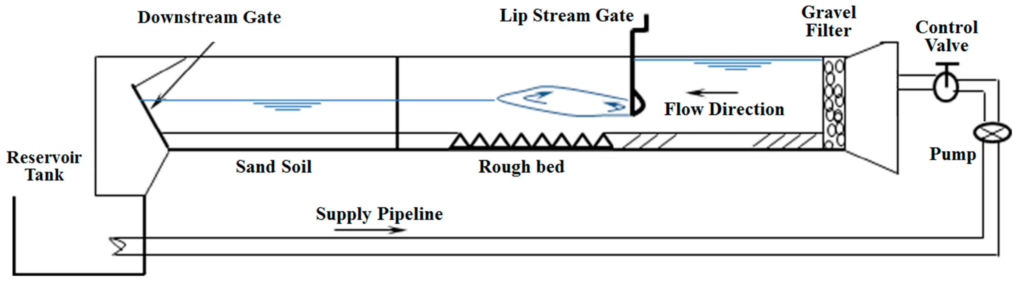
To confirm the performance and reliability of the present simulations, reference experimental data by Ahmed et al. [20] are considered as a benchmark solution for some of the basic parameters of submerged hydraulic jump on smooth bed and macroroughnesses, including a submerged ratio and tailwater ratio (y₃/y₁ and y₄/y₁). For these experiments, a flume with length, width and depth of 24.5, 0.75 and 0.7 m, respectively, was used (see Figure 2). The discharge and water depths were evaluated through an ultrasonic flow meter which was specified at the supply lines and a point-gauge, respectively. A gate with a horizontal basin was used to develop the required supercritical flow and initial depth of the hydraulic jumps. Downstream water depth was controlled by a tailgate to form hydraulic jumps over the rigid bed, and then, the water flowed to the by-pass channel (for more details, see Ahmed et al. [20]).

Although the length of the experimental flume was 24.5 m, in the present study, the length of the flume in the numerical runs was set equal to 4.5 m, to decrease the computational effort decreasing the overall number of the computational cells.

Table 3. Main flow variables for the numerical and physical models (Ahmed et al. [20]).

Models	Bed Type	Q (l/s)	d (cm)	y1 (cm)	u1 (m/s)	Fr1
Numerical and Physical	Smooth	45	5	1.62–3.83	1.04–3.70	1.7–9.3
	T/I = 0.5	45	5	1.61–3.83	1.05–3.71	1.7–9.3
	T/I = 0.25	45	5	1.60–3.84	1.04–3.71	1.7–9.3

shows the main flow variables for the numerical and physical models.

3.3. CFD Analysis

Generally, the application of computational methods is essential for the prediction of entrained air in free surface/two-phase flows. The hydraulic jumps are specified by an extremely turbulent flow zone with a significant amount of entrained air. Therefore, numerical simulations of two-phase flow involving a hydraulic jump were here performed with the help of the commercial CFD software FLOW-3D^® [16]. The FLOW-3D uses the finite volume method in a Cartesian, staggered grid to solve the Reynolds’ average Navier–Stokes (RANS equations. The governing equations are briefly described in tensor notations. Assuming incompressible fluid, the mass conservation equation is expressed as

$$\frac{\partial u_i}{\partial x_i}=0$$

(3)

The momentum conservation equations (Navier–Stokes equations) are:

$$\rho \frac{\partial u_i}{\partial t}+\rho u_j\frac{\partial u_i}{\partial x_j}=-\frac{\partial p}{\partial x_i}+\frac{\partial t_{ji}}{\partial x_j}$$

(4)

Here, u_i and x_i are velocity and position vectors, t is the time, p and ρ denotes the pressure and fluid density and t_ij refers to the viscous stress tensor, expressed by

$$t_{ij}=2\mu s_{ij}$$

(5)

where μ is molecular viscosity and s_ij refers to the strain-rate tensor, defined as

$$s_{ij}=\frac{1}{2}\left(\frac{\partial u_i}{\partial x_j}-\frac{\partial u_j}{\partial x_i}\right)$$

(6)

Note that s_ij = s_ji, so that t_ji = t_ij for simple viscous fluids [28]. The FLOW-3D^® utilizes an advanced algorithm for tracking free-surface flows, called volume of fluid (VOF), and is developed by Hirt and Nichols [29]. The VOF equation is written by the Equation (7):

$$\frac{\partial F}{\partial t}+\frac{1}{V_F}\left[\frac{\partial (F{A}_{x}u)}{\partial x}+\frac{\partial (F{A}_{y}v)}{\partial y}+\frac{\partial (F{A}_{z}w)}{\partial z}\right]=0$$

(7)

Here, F denotes the fraction function. In particular, if a cell is empty, then F = 0, and if a cell is full, then F = 1 [16,30,31]. The free surface is determined at a position related to intermediate amounts of F (usually F = 0.5, but another intermediate amount may be determined by the user).

3.4. Turbulence Model

The Reynolds decomposition is the main tool needed for the extraction of the RANS equations from the instantaneous Navier–Stokes equations. The Reynolds decomposition simplifies the Navier–Stokes equations (see Equation (4)) by the separation of the flow variable (like velocity u) into the mean (time-averaged) component (ū) and the fluctuating component (u’). Thus, we can replace the Navier–Stokes Equation (4) and obtain the average Navier-Stokes equations [32]. The obtained equation includes a nonlinear term that gives rise to turbulence defined as the Reynolds stresses tensor. The Boussinesq hypothesis is used to relate the Reynolds stresses tensor ($-\rho \overline{u_i^{\prime }{u}_j^{\prime }}$) to the mean velocity gradients using an eddy viscosity by the following equation:

$$-\rho \overline{u_i^{\prime }{u}_j^{\prime }}={\epsilon }_{}\left[\frac{1}{2}\left(\frac{\partial U_i}{\partial x_j}-\frac{\partial U_j}{\partial x_i}\right)\right]-\frac{2}{3}k{\delta }_{ij}$$

(8)

Here, U_i denotes the mean velocity component in a Cartesian coordinate system, x_i is the Cartesian space (i, j, k), ε_ij is the eddy viscosity tensor, δ_ij and k are the Kronecker delta and the turbulent kinetic energy, respectively [29]. In present study, the desired turbulence model was RNG k-ε, as suggested in Flow Science, Inc. (New York, NY, USA) [16]. The RNG k-ε is similar to the standard k-ε model even if it contains some refinements. In particular, the RNG k-ε turbulence model has an additional term in its ε equation (see successive Equation (12)) that improves the accuracy for quickly strained and swirling flows and also have good accuracy based on the results of numerical investigations by Carvalho et al. [33], Bayon et al. [34], Daneshfaraz et al. [35], Ghaderi and Abbasi [36] and Ghaderi et al. [37,38]. This model was proposed by Yakhot and Orszag [39] and represents a modified version of the k-ε standard model.

The adopted turbulence scheme is a two-equation model. In particular, the first equation (Equation (9)), which is called turbulent kinetic energy (k), expresses the energy in turbulence. The second equation (Equation (10)), which determines the rate of kinetic energy dissipation, is the turbulent dissipation rate (ε). These equations are presented as follows:

$$\frac{\partial (\rho k)}{\partial t}+\frac{\partial (\rho k{u}_i)}{\partial x_i}=\frac{\partial }{\partial x_j}[{\alpha }_k{\mu }_{eff}\frac{\partial k}{\partial x_j}]+G_k-G_B-\rho \epsilon -Y_M+S_k$$

(9)

$$\frac{\partial (\rho \epsilon )}{\partial t}+\frac{\partial (\rho \epsilon u_i)}{\partial x_i}=\frac{\partial }{\partial x_j}[{\alpha }_{\epsilon }{\mu }_{eff}\frac{\partial \epsilon }{\partial x_j}]+C_{1\epsilon }\frac{\epsilon }{k}(G_k+C_{3\epsilon }{G}_b)-C_{2\epsilon }^{}\rho \frac{{\epsilon }^2}{k}-R_{\epsilon }+S_{\epsilon }$$

(10)

Here, G_k refers to the generation of turbulent kinetic energy caused by the average velocity gradient, G_b denotes the generation of turbulent kinetic energy caused by buoyancy, while S_k and S_ε are source terms. α_k and α_ε are inverse effective Prandtl numbers for k and ε, respectively. μ_eff is the effective viscosity μ_eff = μ + μ_t, being the eddy viscosity.

For the above equation [40,41,42]:

$$R_{\epsilon }=\frac{C_{\mu }\rho {\eta }^3(1-\eta /{\eta }_0){\epsilon }^2}{k(1+\beta {\eta }^3)}$$

(11)

$${\mu }_t=\frac{\rho C_{\mu }{k}^2}{\epsilon }$$

(12)

The constant values for this model are [39]:

C_µ = 0.0845, C_1ε = 1.42, C_2ε = 1.68, C_3ε = 1.0, σ_k = 0.7194, σ_ε = 0.7194, η₀ = 4.38 and β = 0.012.

3.5. Boundary Conditions in the Computational Domain

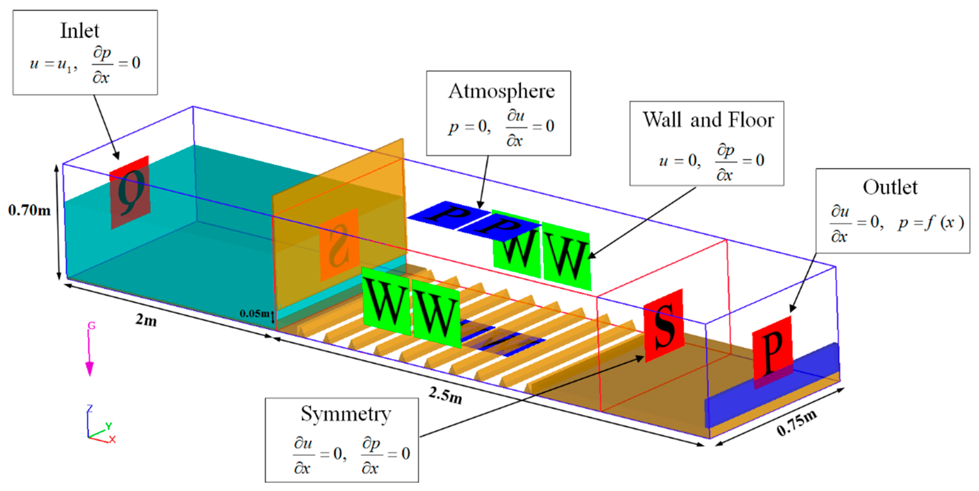
According to Figure 3, the discharge flow rate (Q) equal to the experimental flow exit discharge as the inlet boundary condition, a pressure (P) corresponding to the tailwater depth as the downstream boundary condition were set. The lower bottom (Z) and both boundary lateral sides behave as rigid wall (W). No-slip conditions are expressed as zero tangential and normal velocities (u = v = w = 0, where u, v and w are the velocities in the directions x, y and z, respectively) that were used at the wall boundaries. This boundary condition implies a wall-law velocity profile (the average velocity of turbulent flow at a certain point is proportional to the logarithm of the distance from that point to the boundary of the fluid zone) [16]. For the upper boundary, the atmospheric pressure boundary condition due to the flow to enter and leave the domain as null von Neumann conditions was imposed to all variables except for pressure, which is set to zero. Symmetry (S) was used at the inner boundary conditions as well. Figure 3 shows the boundary conditions governing the simulations.

3.6. Computational Grid and Grid Convergence Analysis

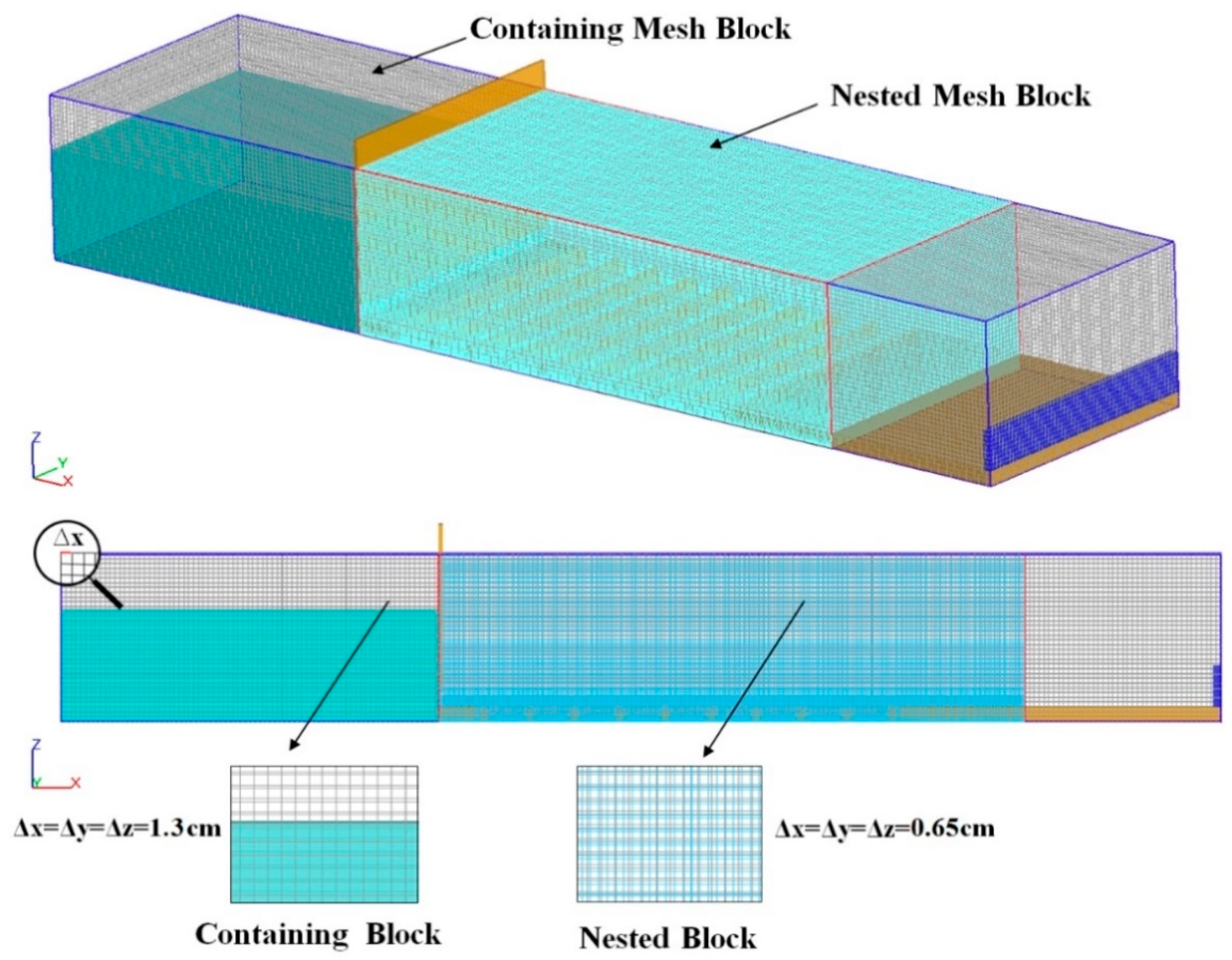
In the present study, the spatial domain meshed with the help of a structured rectangular hexahedral mesh with two mesh blocks was built. In particular, the above mesh blocks include a mesh block for the entire spatial domain and a nested mesh block with refined cells for the area of interest (see Figure 4). By using the Grid Convergence Index (GCI) (specified for the computed y₃/y₁ ratio at Fr₁ = 4.5 obtained from the numerical solution), which is a recommended method for evaluating the discretization error, three various computational meshes were applied to choose the appropriate one [17,34,38,43]. The analysis was performed according to the Richardson extrapolation method [44]. To investigate the effect of the grid size on the accuracy of the results, three meshes were used with fine, medium, and coarse cells, containing 1,285,482 and 2,908,596, and 4,624,586 cells, respectively.

Table 4. Characteristics of the computational grids.

Mesh	Nested Block Cell Size (cm)	Containing Block Cell Size (cm)
1	0.55	1.10
2	0.65	1.30
3	0.85	1.70

shows some characteristics of the computational grids.

The fine-grid convergence index is expressed as [43]

$$GC{I}_{32}^{fine}=\frac{1.25\left|E_{32}\right|}{r_{32}^p-1}$$

(13)

Here, E₃₂ = (f_s2 − f_s3)/f_s2 refers to the relative error between the medium and fine grids, f_s2 and f_s3 are medium and fine grid solutions for y₃/y₁, respectively, and K denotes the local order of accuracy. For the three-grid solutions, K is presented as follows:

$$K=\frac{1}{\ln r_{32}}\ln \frac{(r_{32}^p-1)e_{21}}{(r_{21}^p-1)e_{32}}$$

(14)

where e₂₁ = f_s2 − f_s1, e₃₂ = f_s3 − f_s2 and r₂₁ = G₂/G₁ are the grid refinement factor between the medium and coarse grids, and r₃₂ = G₃/G₂ is the grid refinement factor between the fine and medium grids. The value of f_s1 represents the coarse grid solution and G₁, G₂ and G₃ are the abbreviations of grids. For the three-grid comparisons, G₃ < G₂ < G₁.

Table 5. The numerical results of mesh convergence analysis.

Parameters	Amounts
fs1 (-)	7.15
fs2 (-)	6.88
fs3 (-)	6.19
K (-)	5.61
E32 (%)	10.02
E21 (%)	3.77
GCI21 (%)	3.03
GCI32 (%)	3.57
GCI32/rp GCI21	0.98

summarizes the numerical results of the mesh convergence analysis in the present study. According to this table, the amounts of GCI₂₁ and GCI₃₂ are the relative change from medium to coarse and from coarse to medium mesh, respectively.

Since the GCI amount for the finer grid (GCI₂₁) is small compared to the coarser grid (GCI₃₂), it can be seen that the grid-independent solution is almost obtained and no further mesh modification is required. The computed value of GCI₃₂/r^pGCI₂₁ close to 1 indicates that the solution is within the asymptotic range of convergence. As a result, the cell size was decreased from 0.65 to 0.55 cm and the mesh including a containing block with a cell size of 1.3 cm and a nested block of 0.65 cm was selected (see Figure 4).

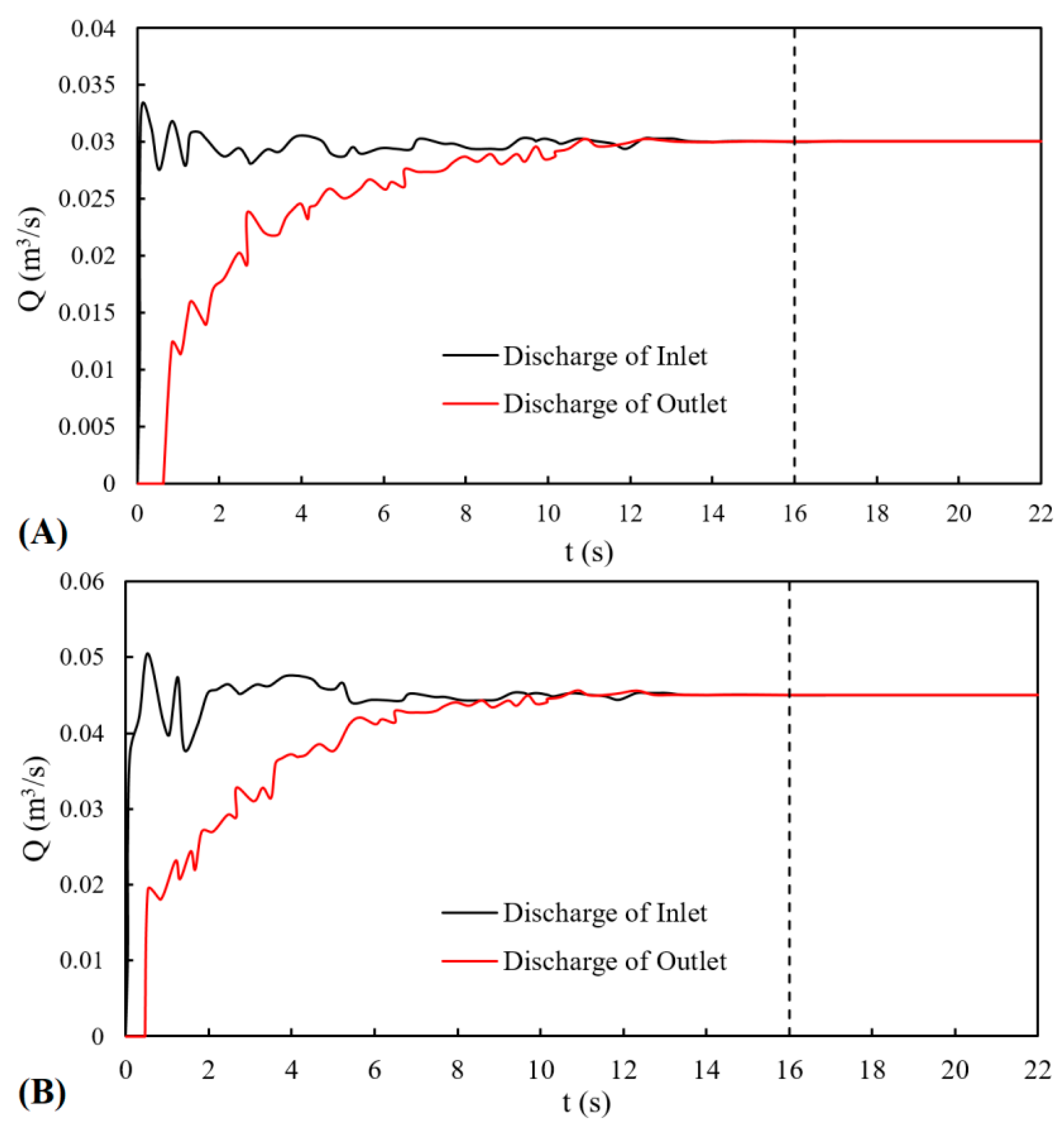
To compute the allowed time-step size, a stability criterion similar to the Courant number was adopted [37]. During the repeat, the time-step size was checked by the stability and convergence criteria, which cause time steps between 0.001 and 0.0016 s. The steady state convergence of the solutions during the simulations was controlled through monitoring the flow discharge changes at the inlet and outlet boundaries conditions. Figure 5 shows that t = 16 s is suitable to reach a near steady state for the adopted two discharges, i.e., Q = 0.03 and 0.045 m³/s. The computational time for the simulations was between 14 and 18 h using a personal computer with eight cores of a CPU (Intel Core i7–7700K @ 4.20 GHz and 16 GB RAM).

4. Results and Discussions

4.1. Validity of the Numerical Model Results

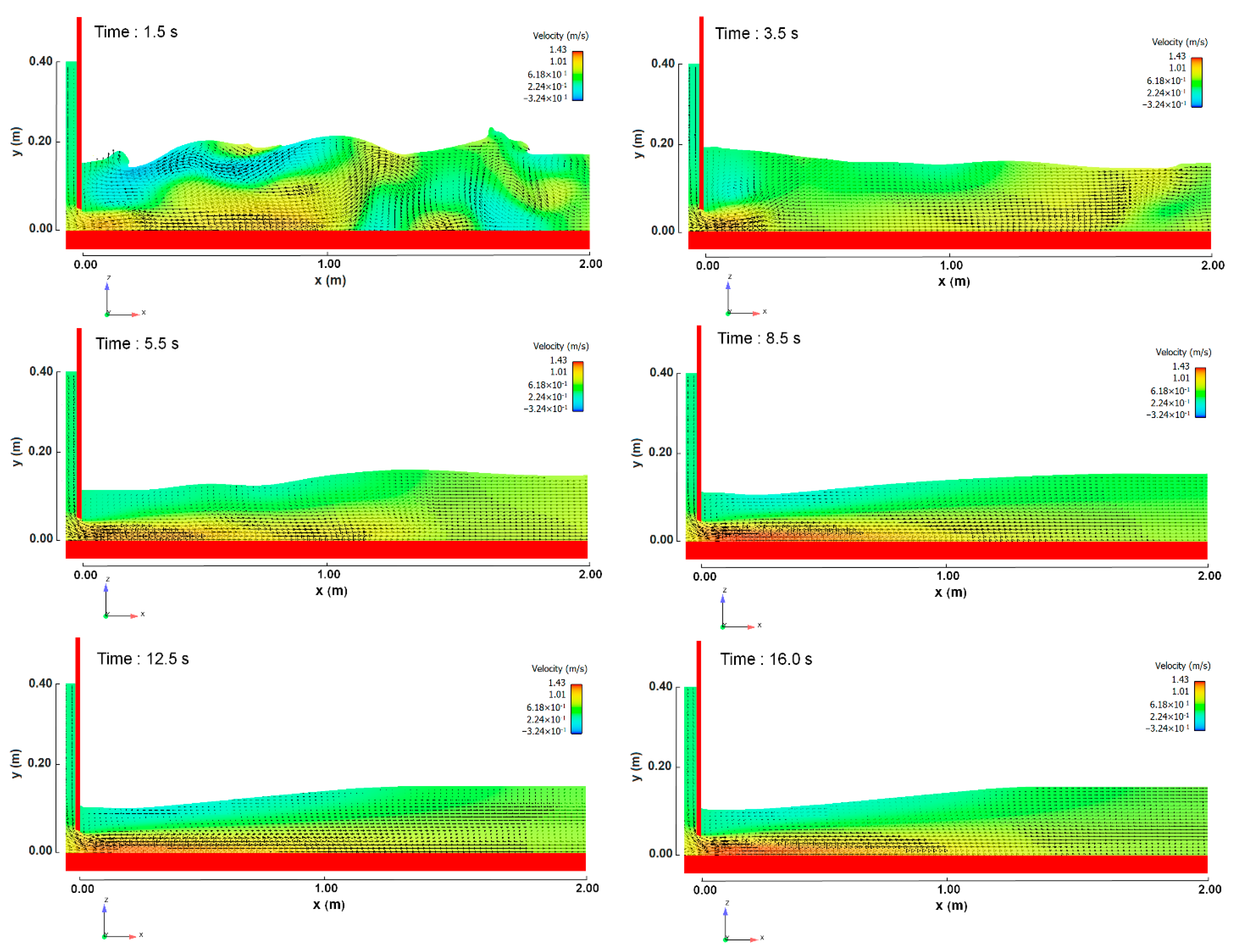
Figure 6 shows some significant time instants of the snapshots of the flow evolution of a numerical simulation of the submerged hydraulic jump on the smooth bed. The surface eddy is formed above the wall jet because of the flow near the bed. The free surface level gradually changes due to the increasing inlet velocity. The depressed water surface elevation at the end of the gate is created by the surface eddy. The stable hydraulic jump was obtained at around t = 16 s. In this time, the water surface variations behind the gate are stable with small fluctuations.

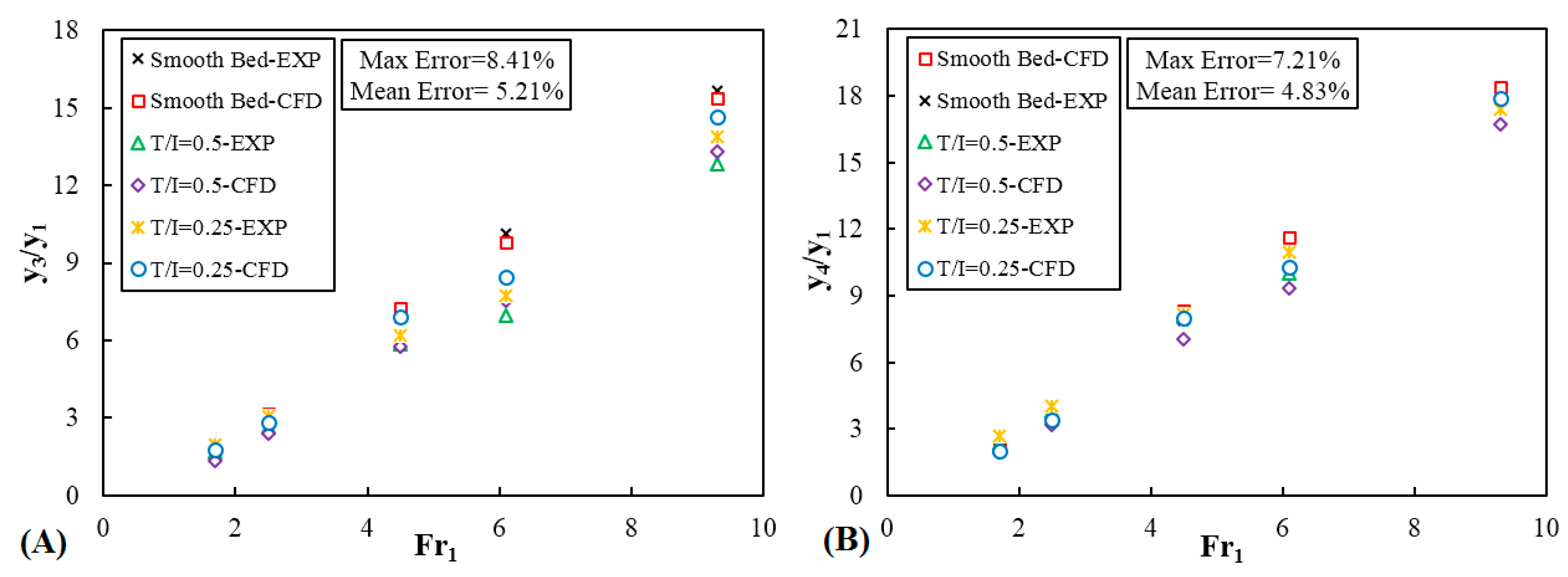
To check the accuracy of the FLOW-3D software, comparisons between numerical and experimental results were performed. Basic parameters including the submerged ratio and tailwater ratio (y₃/y₁ and y₄/y₁) of a submerged hydraulic jump on a smooth bed and with triangular macroroughnesses with T/I = 0.25 and 0.5 were extracted from the numerical simulations and plotted as shown in Figure 7. From the graphs, a strong agreement can be observed between numerical and experimental results by Ahmed et al. [20] as a function of Fr₁. The overall maximum error and mean value of relative error are 8.41 and 4.83%, respectively, which confirms the capability of the numerical model to predict the main properties of a submerged hydraulic jump in terms of water depths.

4.2. Longitudinal Profile of Streamlines

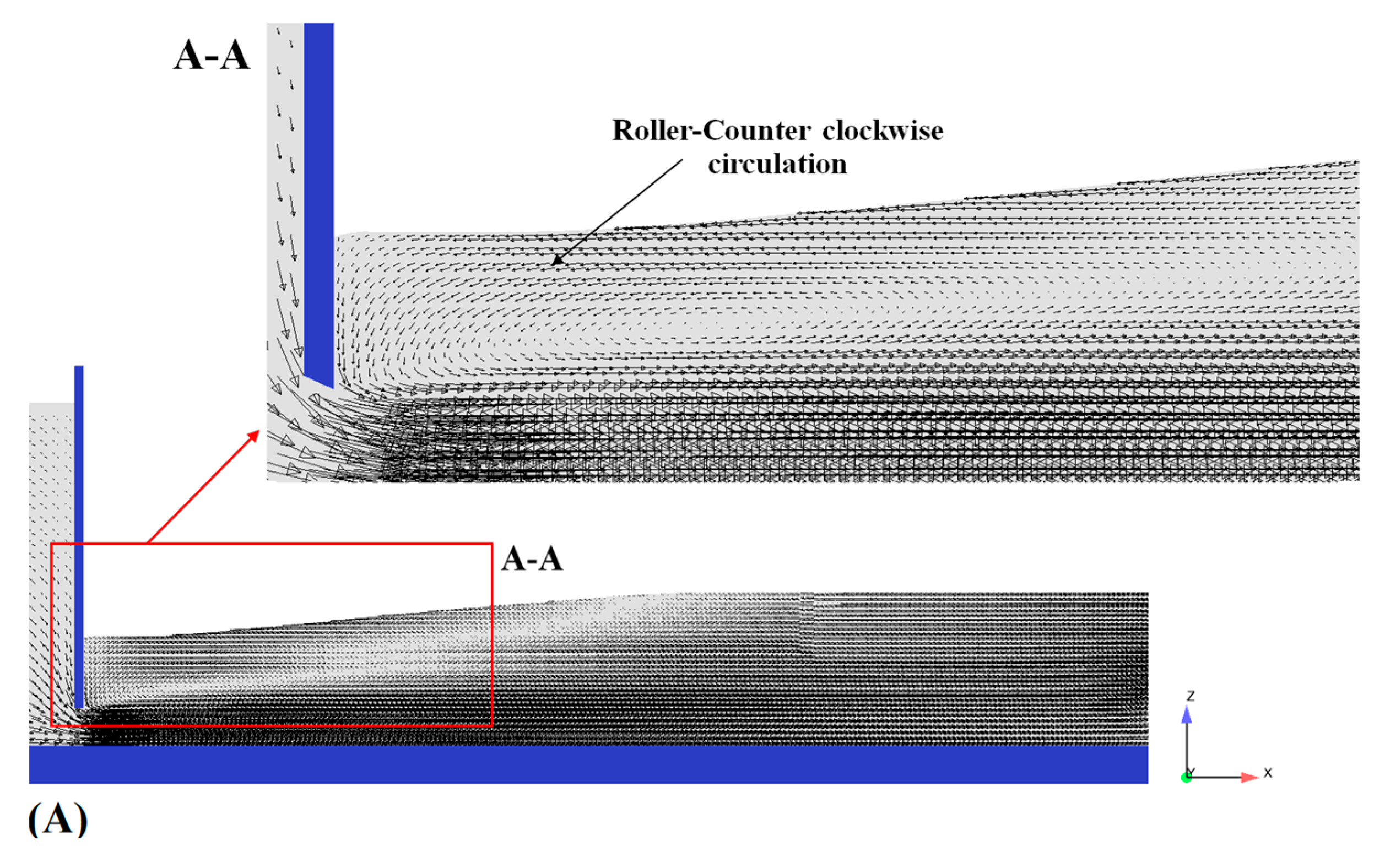
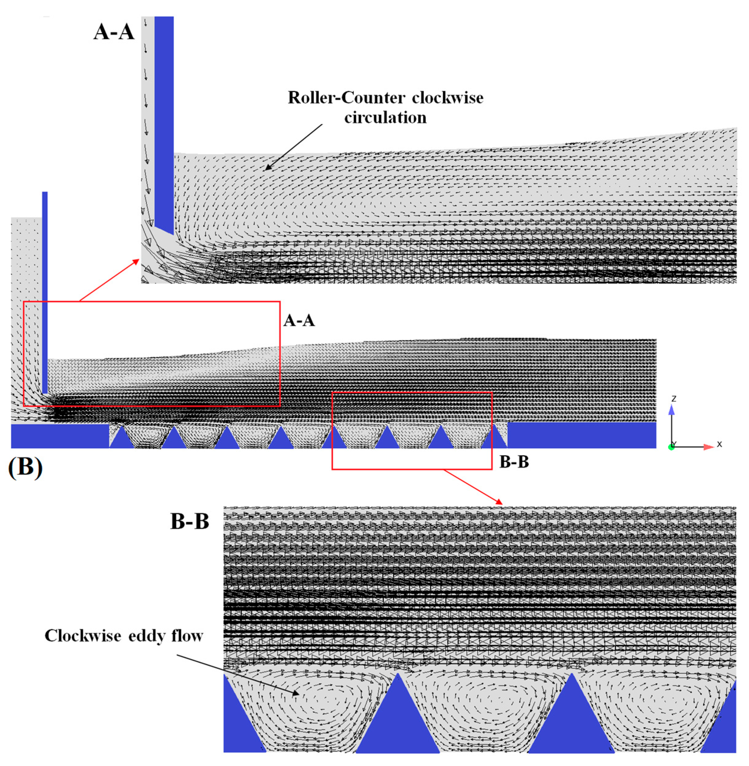
Figure 8 illustrates the longitudinal profile of the velocity vectors passing under the sluice gate for the smooth bed and in the presence of triangular macroroughnesses in a submerged hydraulic jump condition. The simulations indicate that, in the smooth bed, the hydraulic jump includes two main regions: a supercritical flow area in the developed region, where it has a big counter-clockwise circulation in the free surface roller and dissipates the hydraulic energy, and a subcritical flow area with developing open channel flow characteristics (see Figure 8A). It can also be seen that the flow pattern in the sluice gate with a triangular macroroughness in the developed and developing regions is the same in comparison to the smooth bed. In addition, triangular macroroughnesses have formed another clockwise eddy flow in the cavity region between the roughnesses (see Figure 8B).

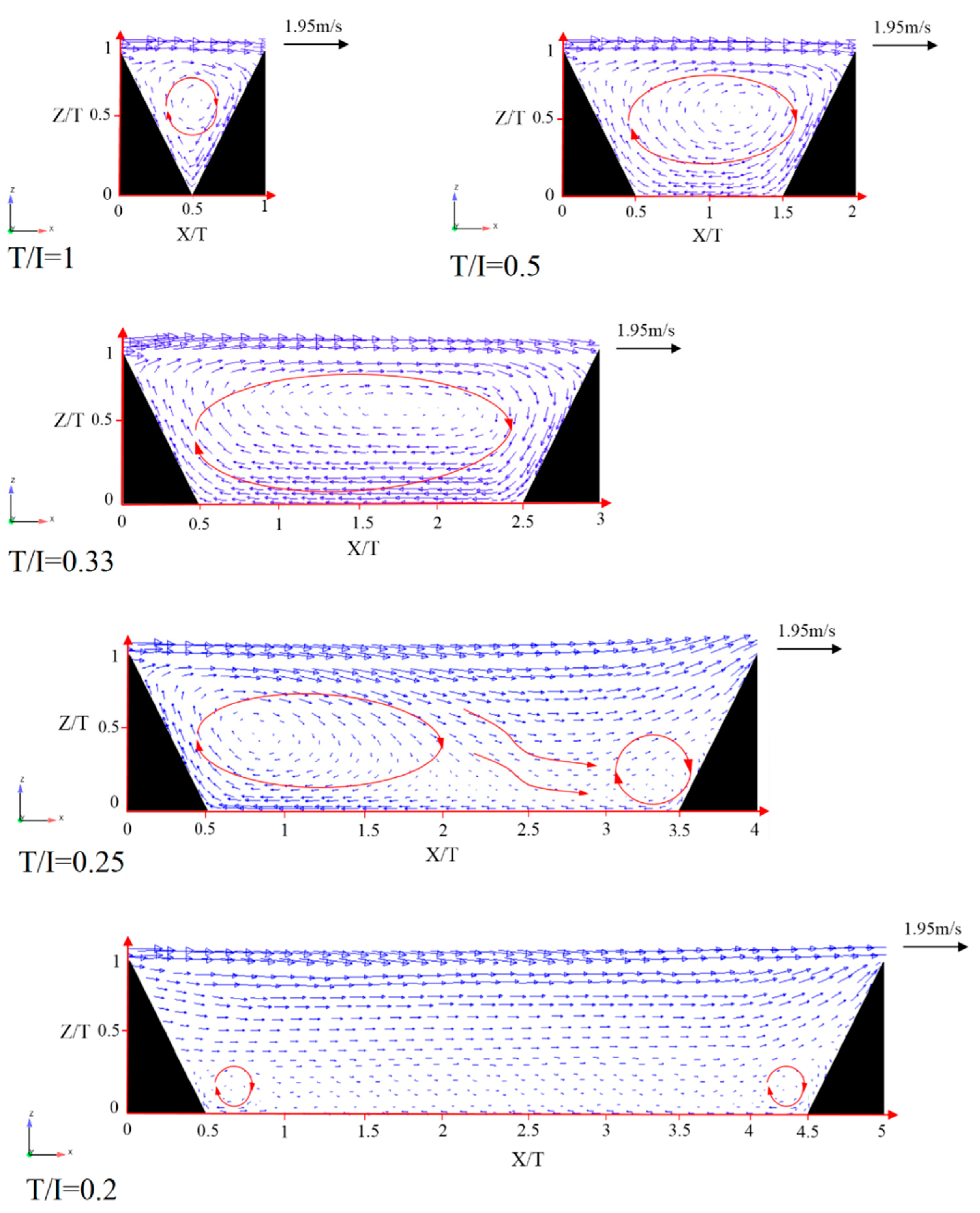
The flow patterns in the cavity region between the triangular elements, considering the distances between the roughnesses, can be generally classified as skimming flow, wake interference and isolated roughness flow [45]. When the distances between the triangular macroroughnesses are relatively closely spaced (e.g., T/I = 1, 0.5 and 0.33), a clockwise eddy in the cavity occurs, where the magnitude of velocity is much smaller than the mean flow velocity in outside the cavity (see Figure 9). In the cavity region, the local mean velocity is about 10% of the mean flow velocity. In skimming flow in the cavity region, there is no significant interaction between the cavity flow and the overlying flow, and the friction coefficient is negative. This is due to the presence of a single recirculation vortex in the current case, as also noticed by [46]. The cavity may be regarded as a dead zone of fluid. With the increasing distance between triangular macroroughnesses (e.g., T/I = 0.25), two eddies of different sizes formed in the cavity region. With one at the upstream and the other at the downstream corners, they interact with each other, as shown in Figure 9. In this situation, the incipient secondary vortices, placed at the upstream corner of the cavity region, mark the beginning of the wake interference flow. Changing the flow pattern in the cavity region from skimming to wake interference flow, an increase in local mean velocity from 39 to 50% of the mean flow velocity appears. In wake interference flow regimes, the vortex was unable to fill the whole cavity and started to act as a three-dimensional vortex liable to be ejected into the main flow. When the triangular macroroughnesses are well apart (e.g., T/I = 0.2), isolated roughness flow occurs where a small eddy formed near the bed and the upstream vortex acts independently of the downstream vortex inside the cavity.

4.3. Velocity Profiles

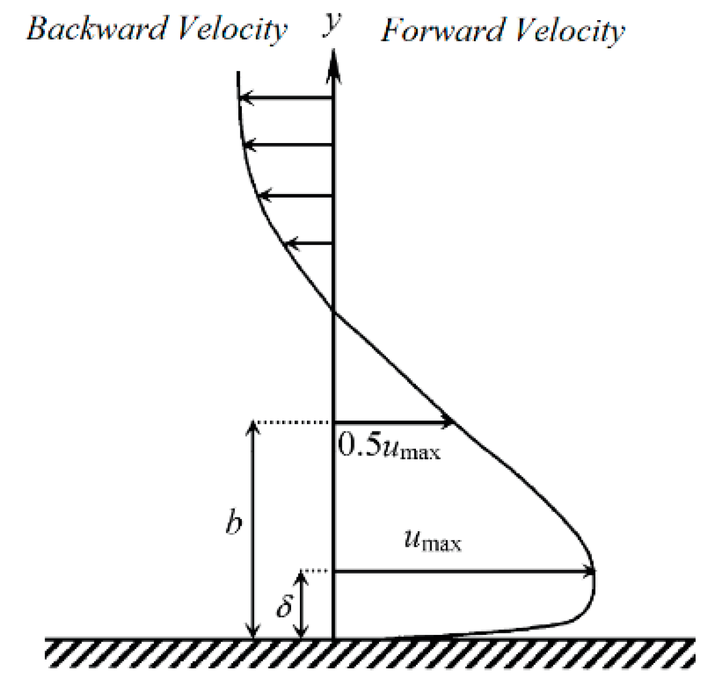
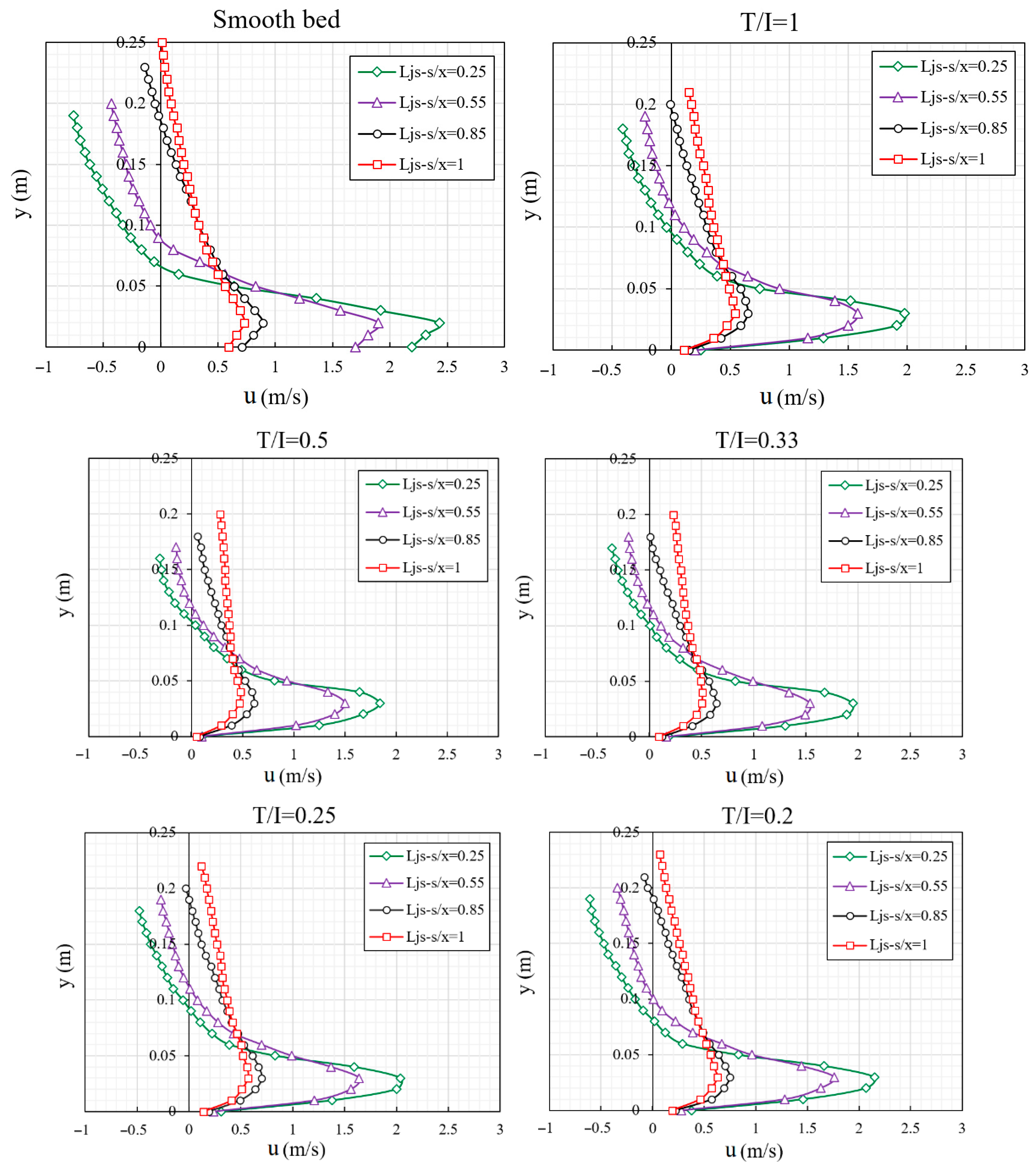
In this section, the velocity profile distributions obtained by measuring the flow velocity at different flow depths and sections on both smooth bed and triangular macroroughnesses were analyzed. The results of the present numerical simulations show that the velocity profile distributions reflect the structure of the wall jet. Hence, with increasing distance x from the beginning of the submerged hydraulic jump, the maximum velocity and the boundary layer growth decrease. To compare the velocity profile distributions in various sections within the jump, δ is the value of y at which the maximum velocity (u_max) and the length scale (b) occur, which is the value of y at which u = 0.5u_max and $\partial$u/$\partial$y < 0 [10,47] (see Figure 10). Figure 11 shows the typical velocity profiles of submerged jump on the smooth bed and triangular macroroughnesses for T/I = 1 and 0.5, respectively.

From the results in Figure 11, as expected, due to the contracted jet below the gate and the flow, velocities decrease at the upper section of the gate opening, since the magnitude of the mean horizontal flow velocity is bigger near the gate. Over time, reverse flow effects increase near the gate and then start to decrease, showing the existence of a stagnation zone on the free surface. The observations also state that the recirculation region occurs near the gate and the negative velocity in the center of the developed region is higher than near the sluice gate. The mean streamwise velocity on the free surface becomes positive in the recovering region. This description is true for both types of beds. For triangular macroroughnesses, as expected, the flow velocity near the bed strongly reduces and becomes negative between two triangles. This is due to a clockwise recirculation zone that exists the space between two macroroughnesses (see Figure 8). Despite a clockwise recirculation, the length of the submerged jump, the submerged depth, and the tailwater depth decrease by about 19.68, 20.87 and 23.34% as a mean, respectively. In Figure 12, the velocity distributions are presented at three sections during the submerged hydraulic jump. These sections are the same for each arrangement of roughness and were measured on top of the roughness elements, i.e., y = 0. The values of x and L_js-s represent the distance from the sluice gate and hydraulic jump length from the smooth bed, respectively.

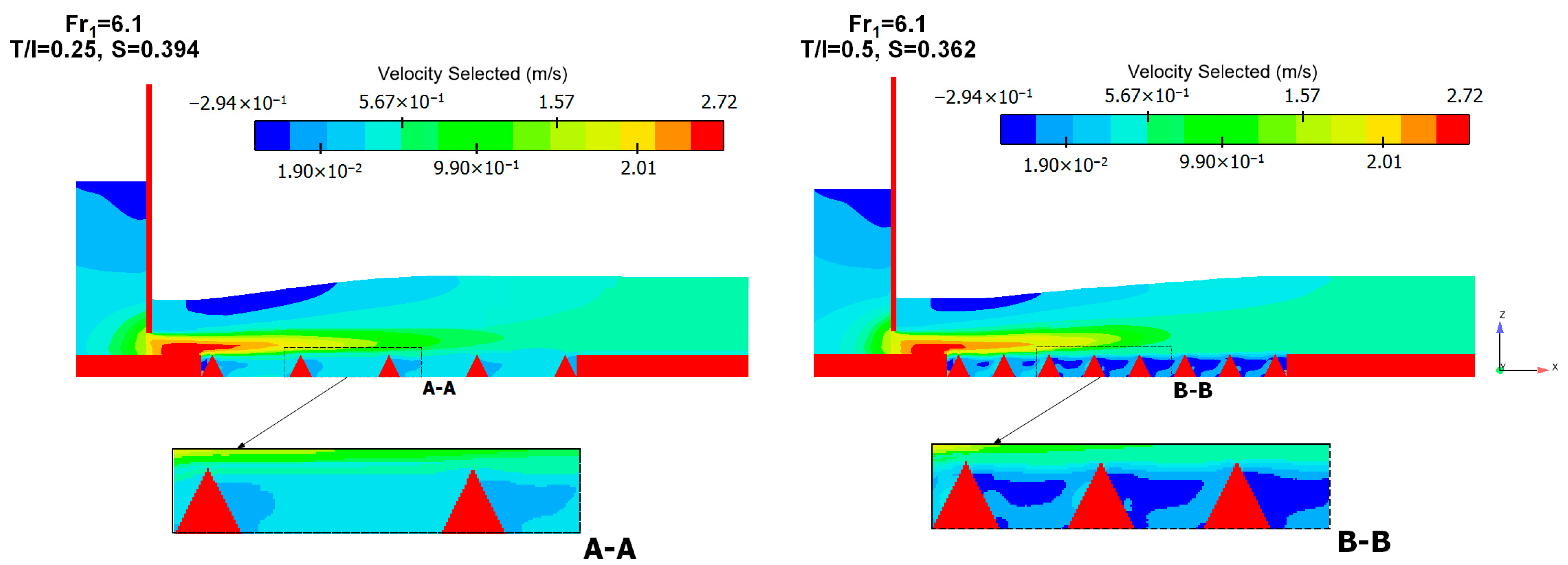
When the distance between the triangular macroroughnesses is long enough, the velocity distribution has recovered by the time that the flow arrives at the next roughness. However, in the short distance, the flow arrives at the next roughness without adequate recovery of the velocity distribution. Hence, with decreasing distance between the macroroughnesses, the rate of increase in the frictional coefficient decreases. As shown in Figure 13, the main velocity in the downstream of each macroroughnesses is low and usually negative. Then, it gradually increases further downstream while the main velocity increases markedly in the region upstream of the macroroughnesses. By comparing the distance between the macroroughnesses, the main velocity at T/I = 0.25 is bigger than T/I = 0.50, despite the inlet Froude number (Fr₁) being the same. The reason can be explained by the fact that the mean velocity cannot be fully developed in a shorter distance between macroroughnesses.

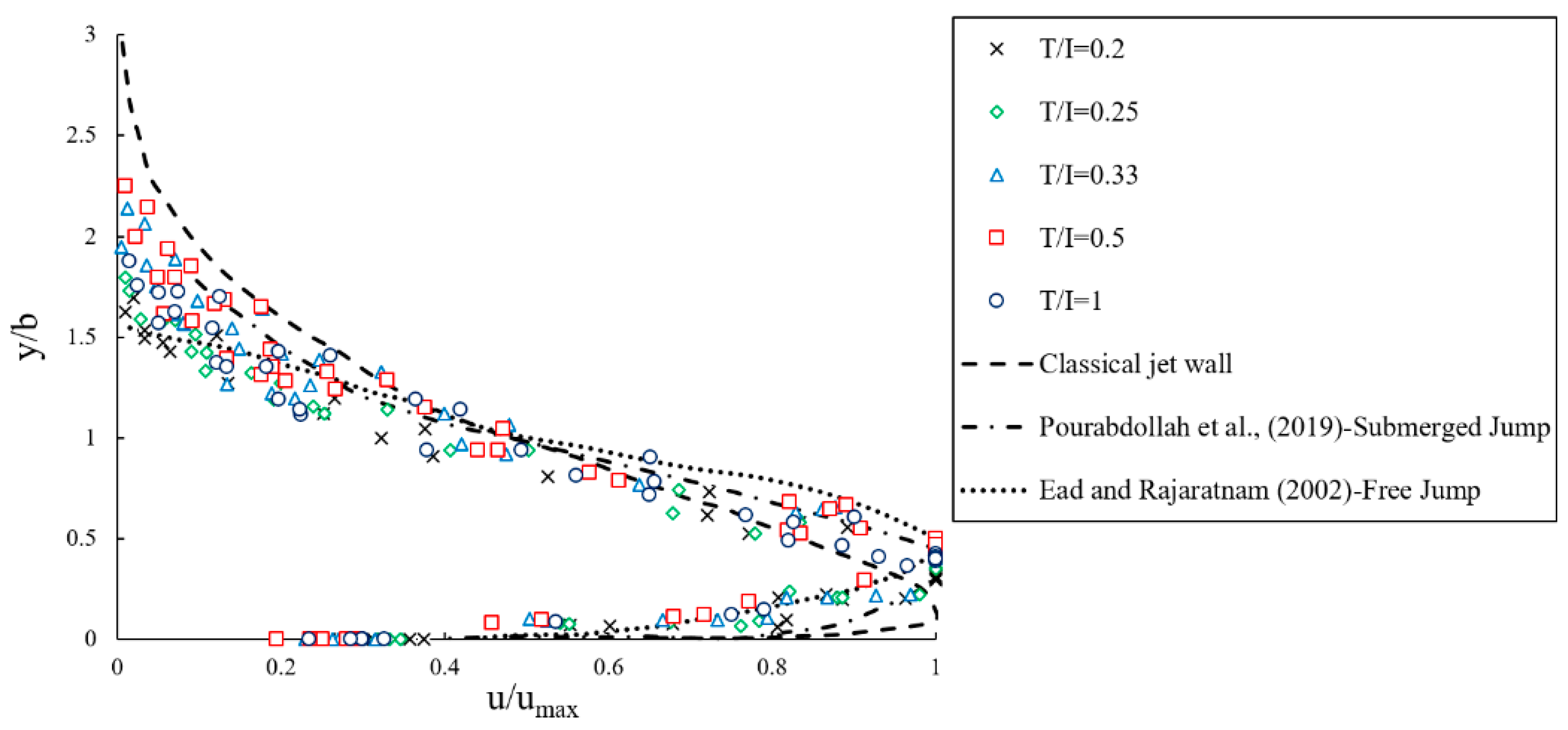
It can be observed from Figure 13 that in the developed region with triangular macroroughnesses, the size of the recirculating zone reduces and does not reach the sluice gate due to the interaction with the vortex of the vertical axis. On the opposite, the region occupied by the forward velocity increases close to the sluice gate and decreases the backward velocity in the middle of the recirculating zone. Figure 14 presents a consolidated plot of all the data simulation for the horizontal velocity distribution in the submerged hydraulic jump given by the ratio of y/b versus u/u_max. The simulations are compared with the classical jet wall and the data from experiments on submerged and free hydraulic jumps conducted by Pourabdollah et al. [48] and Ead and Rajaratnam [10], respectively. It is observed that the velocity profiles in the forward flow are similar for all the Froude numbers and the change in distance between the macroroughnesses. However, they are somewhat different from the profile for the classical jet wall, which is a plane turbulent jet wall growing in a large ambient [49,50]. Additionally, the maximum flow velocity of the submerged hydraulic jump occurred at a less depth compared to a previous study on a free hydraulic jump conducted by Ead and Rajaratnam [10]. Increasing the distance between the macroroughnesses will reduce the position of maximum velocity, indicating the reduction in the thickness of the inner layer (δ) of the horizontal velocity distribution.

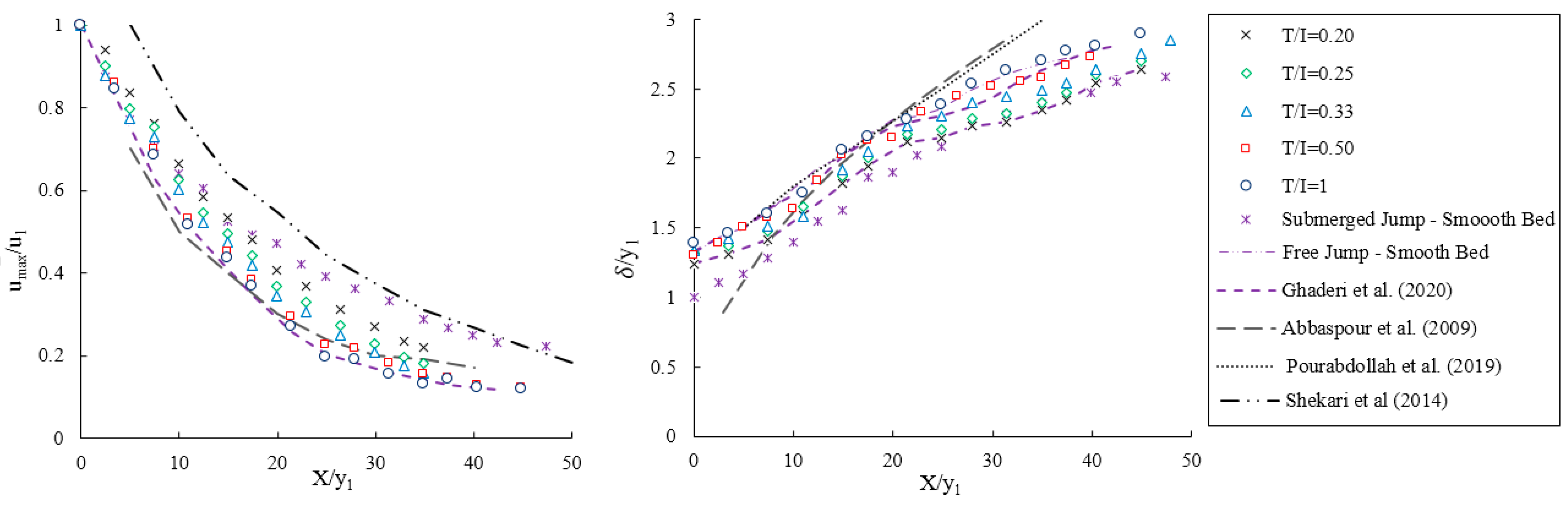
The spatial variation of values (u_max/u₁) and (δ⁄y₁) in submerged jumps over smooth bed and macroroughnesses are illustrated in Figure 15. In this figure, X represents the distance related to start of the hydraulic jump. The results are compared with the data reported by Ghaderi et al. [17] and Abbaspour et al. [12] in free jumps on a rough bed, Shekari et al. [51] and Pourabdollah et al. [48] in submerged jumps on a smooth bed. In the macroroughnesses, the maximum flow velocity before the jump is more than in the smooth bed. However, after the jump, these values are higher in the smooth bed for the submerged jump. By increasing the distance between the roughnesses, the maximum flow velocity is increased. In the macroroughnesses, the ratio (u_max/u₁) at a specified X in the submerged jump is higher than in the free jump. This finding agrees with a previous study by Pourabdollah et al. [48]. For both types of bed (smooth bed and macroroughnesses), the maximum velocity distance from the bed is decreased due to the increasing depth and eddy flow. The results of the present study are in good agreement with the data reported by Abbaspour et al. [12] and Pourabdollah et al. [48].

4.4. Bed Shear Stress

The application of the macroroughnesses is to increase the bed shear stress [10]. The bed shear stress coefficient (ε) is calculated as shown in Equation (15) (from Rajaratnam [24]):

$$\epsilon =\frac{F_{\tau }}{0.5\gamma b{y}_1^2}$$

(15)

where γ is the specific weight of water, F_τ is shear force per unit width. This quantity can be obtained using Equation (16):

$$F_{\tau }=(P_1-P_2)+(M_1-M_2)$$

(16)

Here, P₁, P₂, M₁ and M₂ are the pressure and momentum before and after the jump, respectively [52]. The bed shear stress coefficient (ε) for the hydraulic jump on the smooth bed and macroroughnesses was calculated on the basis of the following equations, respectively [10]:

$$\epsilon =0.16F{r}_1^2-0.8F{r}_1+1$$

(17)

$$\epsilon ={(F{r}_1-1)}^2$$

(18)

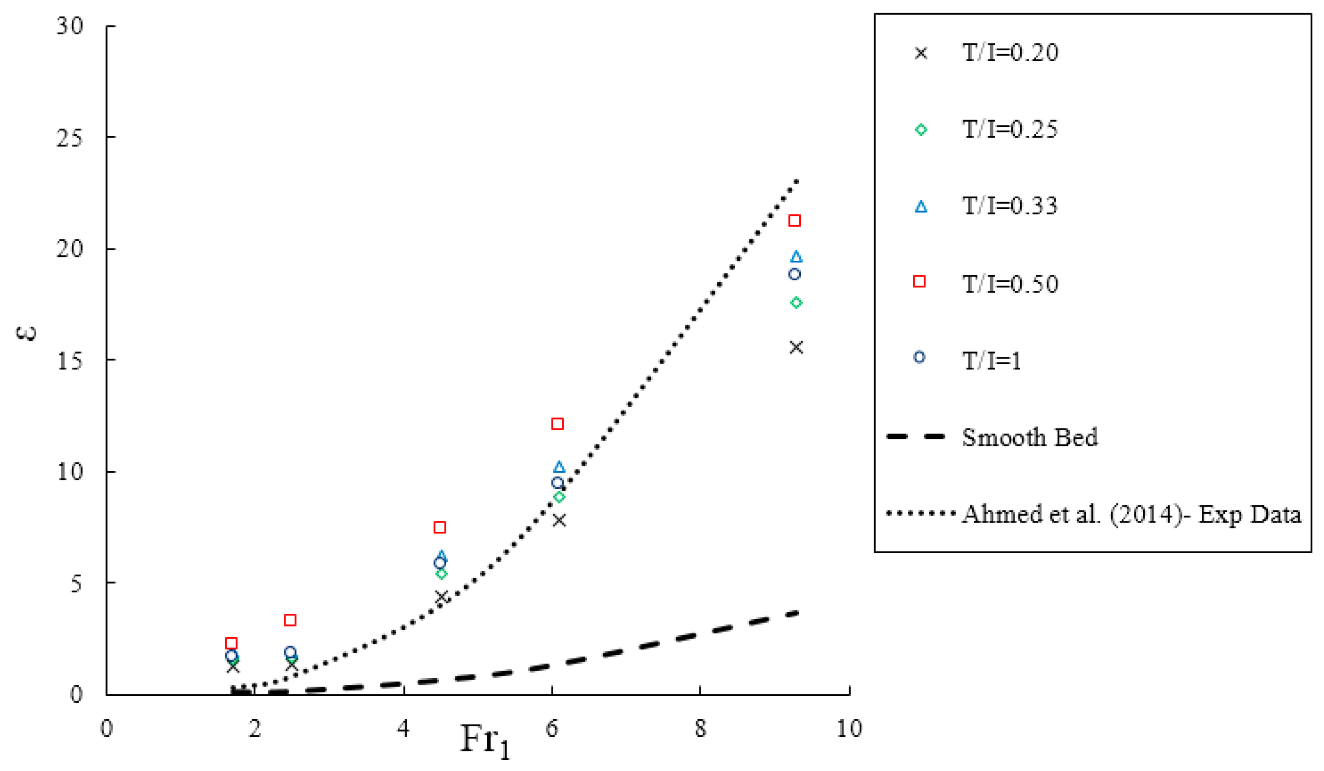
The value of (ε) was obtained by Equation (15) and it was plotted against the inlet Froude number (Fr₁) in Figure 16. The results of this study were compared with prior research data by Ahmed et al. [20] and their experimental data.

According to Figure 16, increasing the inlet Froude number (Fr₁), the shear stress coefficient (ε) increases. The value of ε of the submerged jump on the triangular macroroughnesses is greater than the one obtained for smooth bed. With the increasing distance of roughness elements, the highest and lowest shear stress occurs at T/I = 0.50 and 0.20, respectively, in comparison to other ratios. It can be stated that there was a generally good agreement between the simulations of this study and the results reported by Ahmed et al. [20]. In general, based on the results drawn from the present study, the following equation for the bed shear stress coefficient on the triangular macroroughnesses was obtained:

$$\epsilon =0.523F{r}_1^{1.605}\to (R^2=0.957)$$

(19)

4.5. Turbulent Kinetic Energy (TKE) and Energy Loss

The turbulent kinetic energy (TKE) is a function of the average velocity values in the three directions (x, y, z) and is an important index to reflect the energy loss between two sections of the flow. TKE is characterized by measuring the root-mean-square of the velocity fluctuations [1]. Considering the continuous values of velocities in the flow direction (u₁, u₂, u₃, …, u_n), the value of the root mean square velocity, u_rms, is obtained as

$$u_{rms}=\sqrt{1/n(u_1^2+u_2^2+u_3^2+\dots +u_n^2)}$$

(20)

Then, TKE is calculated as

$$TKE=1/2(u_{rms}^2+v_{rms}^2+w_{rms}^2)$$

(21)

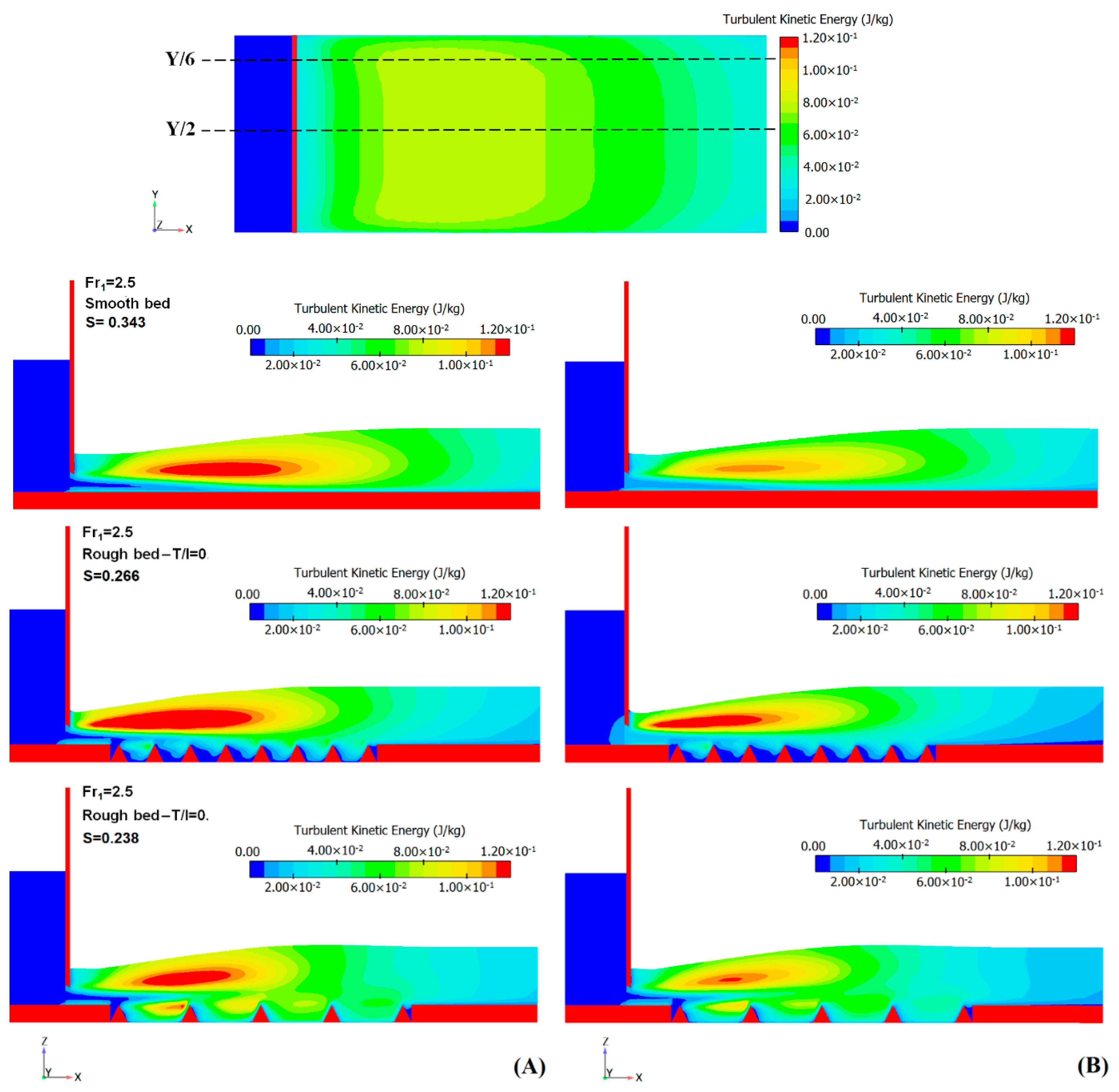
When the energy loss is fierce (or insufficient) for turbulent flow, the values of TKE would increase up (or decrease down). The longitudinal sections are adopted to describe the TKE variation. As shown in Figure 17A, the turbulence region on a smooth bed is created with the distance from a sluice gate and occurs near free surface roller area, thus resulting in hysteretic energy loss and a wide sweep region on the length of the smooth bed. Whereas on the triangular macroroughnesses, the region of turbulence begins near a sluice gate with greater intensity and a limited sweep region that is the result of a counter-clockwise circulating in free surface roller and clockwise eddy flow in the space between the roughness. By increasing the distance between the roughnesses, the intensity of the turbulence region is reduced.

Observe also from Figure 17A,B that the peak of the TKE increases in elevation as Y decreases from the centerline of the channel (Y/2); indeed, the overall values of TKE close to the wall (Y/6) are smaller than in the centerline section (Y/2). This is essentially due to the separated boundary-layer from the returning flow near the free surface, which is the effect in the intensity of TKE and discussed by de Dios et al. [53]. The energy loss through the submerged hydraulic jump (E_L) is equal to the difference between the specific energy before and after the submerged jump (E₃ − E₄):

$$\frac{E_L}{E_3}=\frac{E_3-E_4}{E_3}=\frac{(y_3+V_3^2/2g)-(y_4+V_4^2/2g)}{(y_3+V_3^2/2g)}$$

(22)

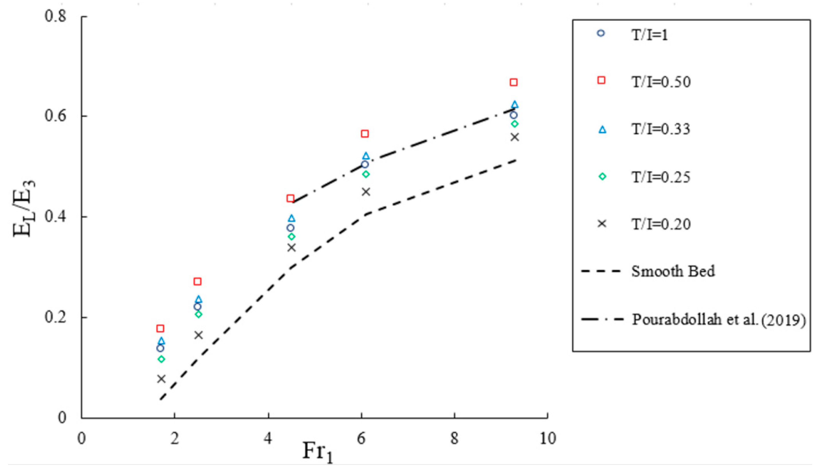
where y₃ and y₄ are the submerged and tailwater depths in the submerged jump, and V₃ and V₄ are the flow velocities before and after the submerged jump, respectively [48]. In Figure 18, the relative energy loss (E_L/E₃) was plotted against the inlet Froude numbers (Fr₁) for smooth bed and various types of triangular macroroughnesses.

Figure 18 illustrates that E_L/E₃ increases with the increasing inlet Froude number (Fr₁). The results stated that, for the same Froude number, the energy loss through the jump on a triangular macroroughnesses with different ratio was greater than the smooth bed. The highest E_L/E₃ occurs for T/I = 0.50 in the submerged jump compared to the values of T/I. The reason for this, with increasing roughness distance, is due to the fact that the vortices created between the roughness decreases and become closer to the smooth bed. The results of this study compared with the results of Pourabdollah et al. [48], showing a good agreement between numerical simulations and experimental results. The following equation allows for the prediction of the relative energy loss with a good correlation coefficient:

$$\frac{E_L}{E_3}=-0.006F{r}_1^2+0.122F{r}_1-0.078\to R^2=0.996$$

(23)

5. Conclusions

The present paper presented and discussed the characteristics of submerged hydraulic jump including the longitudinal profile of streamlines, flow patterns in the cavity region, horizontal velocity profiles, streamwise velocity distribution, thickness of the inner layer, bed shear stress coefficient, turbulent kinetic energy (TKE) and energy loss over triangular macroroughnesses. These characteristics were numerically investigated using the FLOW-3D^® model. The volume of fluid (VOF) method to simulate free surface and the turbulence RNG k-ε model are implemented. To validate the present model, comparisons between numerical simulations and experimental results were performed for the smooth bed and triangular macroroughnesses. The following results of the present study can be drawn:

• The flow patterns in the triangular macroroughnesses in the developed and developing regions are the same with smaller areas in comparison with the smooth bed in submerged hydraulic jump conditions. The triangular macroroughnesses lead to the formation of another clockwise eddy flow in the cavity region between the macroroughnesses.
• For distances equal to T/I = 1, 0.5 and 0.33, the velocity vector distribution displays a clockwise eddy in the cavity region, where the magnitude of velocity is much smaller than the mean flow velocity. Increasing the distance between triangular macroroughnesses (T/I = 0.25 and 0.2), two eddies of different sizes are formed in the cavity region.
• When the distance between the triangular macroroughnesses is long enough, the velocity distribution has recovered by the time that the flow arrives at the next roughness. However, in the short distance, the flow arrives at the next roughness without adequate recovery of the velocity distribution. Hence, with decreasing distance between macroroughnesses, the rate of increase in the frictional coefficient decreases.
• In the triangular macroroughnesses, the maximum velocity at a specified section in the submerged jump leads to higher values than the free jump. In addition, for both types of bed (smooth and rough) in the submerged jump, the maximum velocity distance from the bed is decreased due to increasing depth and eddy flow. In the submerged jump, the boundary layer thickness is less than the free jump.
• The turbulence region on the smooth bed is created with the distance from the gate and occurs near free surface roller area, whereas on the macroroughnesses, the turbulence begins near a gate with greater intensity and limited sweep region that is the result of a counterclockwise circulating in free surface roller and clockwise eddy flow in the space between the macroroughnesses.
• The bed shear stress coefficient and energy loss of the submerged jump on the triangular macroroughnesses is larger than that found on the smooth bed that increased with the increase in inlet Froude numbers. The highest and lowest bed shear stress coefficient and energy loss occur in T/I = 0.50 and 0.20 with the increasing distance of roughness elements compared to a smooth bed.
• The reduction in the length of the jump and the submerged and tailwater depths given by the presence of triangular macroroughnesses with near-roughness elements can be used in the design of stilling basins with a resulting decrease in their size, i.e., length and height.

Generally, CFD models are fairly well able to simulate predictions of properties of submerged jump, considering various hydraulic conditions and geometrical arrangements. Flow patterns in the cavity region, streamwise and horizontal velocity distribution, bed shear stress coefficient, TKE and the energy loss of hydraulic jump can be simulated with a numerical method. However, the study of the macroroughnesses dimension and various arrangements on the alteration of the flow field and cavity flow as a future work remains an issue to be faced.

References

- White, F.M. Viscous Fluid Flow, 2nd ed.; McGraw-Hill University of Rhode Island: Montreal, QC, Canada, 1991. [Google Scholar]
- Launder, B.E.; Rodi, W. The turbulent wall jet. Prog. Aerosp. Sci. 1979, 19, 81–128. [Google Scholar] [CrossRef]
- McCorquodale, J.A. Hydraulic jumps and internal flows. In Encyclopedia of Fluid Mechanics; Cheremisinoff, N.P., Ed.; Golf Publishing: Houston, TX, USA, 1986; pp. 120–173. [Google Scholar]
- Federico, I.; Marrone, S.; Colagrossi, A.; Aristodemo, F.; Antuono, M. Simulating 2D open-channel flows through an SPH model. Eur. J. Mech. B Fluids 2012, 34, 35–46. [Google Scholar] [CrossRef]
- Khan, S.A. An analytical analysis of hydraulic jump in triangular channel: A proposed model. J. Inst. Eng. India Ser. A 2013, 94, 83–87. [Google Scholar] [CrossRef]
- Mortazavi, M.; Le Chenadec, V.; Moin, P.; Mani, A. Direct numerical simulation of a turbulent hydraulic jump: Turbulence statistics and air entrainment. J. Fluid Mech. 2016, 797, 60–94. [Google Scholar] [CrossRef]
- Daneshfaraz, R.; Ghahramanzadeh, A.; Ghaderi, A.; Joudi, A.R.; Abraham, J. Investigation of the effect of edge shape on characteristics of flow under vertical gates. J. Am. Water Works Assoc. 2016, 108, 425–432. [Google Scholar] [CrossRef]
- Azimi, H.; Shabanlou, S.; Kardar, S. Characteristics of hydraulic jump in U-shaped channels. Arab. J. Sci. Eng. 2017, 42, 3751–3760. [Google Scholar] [CrossRef]
- De Padova, D.; Mossa, M.; Sibilla, S. SPH numerical investigation of characteristics of hydraulic jumps. Environ. Fluid Mech. 2018, 18, 849–870. [Google Scholar] [CrossRef]
- Ead, S.A.; Rajaratnam, N. Hydraulic jumps on corrugated beds. J. Hydraul. Eng. 2002, 128, 656–663. [Google Scholar] [CrossRef]
- Tokyay, N.D. Effect of channel bed corrugations on hydraulic jumps. In Proceedings of the World Water and Environmental Resources Congress 2005, Anchorage, AK, USA, 15–19 May 2005; pp. 1–9. [Google Scholar]
- Abbaspour, A.; Dalir, A.H.; Farsadizadeh, D.; Sadraddini, A.A. Effect of sinusoidal corrugated bed on hydraulic jump characteristics. J. Hydro-Environ. Res. 2009, 3, 109–117. [Google Scholar] [CrossRef]
- Shafai-Bejestan, M.S.; Neisi, K. A new roughened bed hydraulic jump stilling basin. Asian J. Appl. Sci. 2009, 2, 436–445. [Google Scholar] [CrossRef] [Green Version]
- Izadjoo, F.; Shafai-Bejestan, M. Corrugated bed hydraulic jump stilling basin. J. Appl. Sci. 2007, 7, 1164–1169. [Google Scholar] [CrossRef]
- Nikmehr, S.; Aminpour, Y. Numerical Simulation of Hydraulic Jump over Rough Beds. Period. Polytech. Civil Eng. 2017, 64, 396–407. [Google Scholar] [CrossRef]
- Flow Science Inc. FLOW-3D V 11.2 User’s Manual; Flow Science Inc.: Santa Fe, NM, USA, 2016. [Google Scholar]
- Ghaderi, A.; Dasineh, M.; Aristodemo, F.; Ghahramanzadeh, A. Characteristics of free and submerged hydraulic jumps over different macroroughnesses. J. Hydroinform. 2020, 22, 1554–1572. [Google Scholar] [CrossRef]
- Elsebaie, I.H.; Shabayek, S. Formation of hydraulic jumps on corrugated beds. Int. J. Civil Environ. Eng. IJCEE–IJENS 2010, 10, 37–47. [Google Scholar]
- Samadi-Boroujeni, H.; Ghazali, M.; Gorbani, B.; Nafchi, R.F. Effect of triangular corrugated beds on the hydraulic jump characteristics. Can. J. Civil Eng. 2013, 40, 841–847. [Google Scholar] [CrossRef]
- Ahmed, H.M.A.; El Gendy, M.; Mirdan, A.M.H.; Ali, A.A.M.; Haleem, F.S.F.A. Effect of corrugated beds on characteristics of submerged hydraulic jump. Ain Shams Eng. J. 2014, 5, 1033–1042. [Google Scholar] [CrossRef] [Green Version]
- Viti, N.; Valero, D.; Gualtieri, C. Numerical simulation of hydraulic jumps. Part 2: Recent results and future outlook. Water 2019, 11, 28. [Google Scholar] [CrossRef] [Green Version]
- Gumus, V.; Simsek, O.; Soydan, N.G.; Akoz, M.S.; Kirkgoz, M.S. Numerical modeling of submerged hydraulic jump from a sluice gate. J. Irrig. Drain. Eng. 2016, 142, 04015037. [Google Scholar] [CrossRef]
- Jesudhas, V.; Roussinova, V.; Balachandar, R.; Barron, R. Submerged hydraulic jump study using DES. J. Hydraul. Eng. 2017, 143, 04016091. [Google Scholar] [CrossRef]
- Rajaratnam, N. The hydraulic jump as a wall jet. J. Hydraul. Div. 1965, 91, 107–132. [Google Scholar] [CrossRef]
- Hager, W.H. Energy Dissipaters and Hydraulic Jump; Kluwer Academic Publisher: Dordrecht, The Netherlands, 1992; pp. 185–224. [Google Scholar]
- Long, D.; Steffler, P.M.; Rajaratnam, N. LDA study of flow structure in submerged Hydraulic jumps. J. Hydraul. Res. 1990, 28, 437–460. [Google Scholar] [CrossRef]
- Chow, V.T. Open Channel Hydraulics; McGraw-Hill: New York, NY, USA, 1959. [Google Scholar]
- Wilcox, D.C. Turbulence Modeling for CFD, 3rd ed.; DCW Industries, Inc.: La Canada, CA, USA, 2006. [Google Scholar]
- Hirt, C.W.; Nichols, B.D. Volume of fluid (VOF) method for the dynamics of free boundaries. J. Comput. Phys. 1981, 39, 201–225. [Google Scholar] [CrossRef]
- Pourshahbaz, H.; Abbasi, S.; Pandey, M.; Pu, J.H.; Taghvaei, P.; Tofangdar, N. Morphology and hydrodynamics numerical simulation around groynes. ISH J. Hydraul. Eng. 2020, 1–9. [Google Scholar] [CrossRef]
- Choufu, L.; Abbasi, S.; Pourshahbaz, H.; Taghvaei, P.; Tfwala, S. Investigation of flow, erosion, and sedimentation pattern around varied groynes under different hydraulic and geometric conditions: A numerical study. Water 2019, 11, 235. [Google Scholar] [CrossRef] [Green Version]
- Zhenwei, Z.; Haixia, L. Experimental investigation on the anisotropic tensorial eddy viscosity model for turbulence flow. Int. J. Heat Technol. 2016, 34, 186–190. [Google Scholar]
- Carvalho, R.; Lemos Ramo, C. Numerical computation of the flow in hydraulic jump stilling basins. J. Hydraul. Res. 2008, 46, 739–752. [Google Scholar] [CrossRef]
- Bayon, A.; Valero, D.; García-Bartual, R.; López-Jiménez, P.A. Performance assessment of Open FOAM and FLOW-3D in the numerical modeling of a low Reynolds number hydraulic jump. Environ. Model. Softw. 2016, 80, 322–335. [Google Scholar] [CrossRef]
- Daneshfaraz, R.; Ghaderi, A.; Akhtari, A.; Di Francesco, S. On the Effect of Block Roughness in Ogee Spillways with Flip Buckets. Fluids 2020, 5, 182. [Google Scholar] [CrossRef]
- Ghaderi, A.; Abbasi, S. CFD simulation of local scouring around airfoil-shaped bridge piers with and without collar. Sādhanā 2019, 44, 216. [Google Scholar] [CrossRef] [Green Version]
- Ghaderi, A.; Daneshfaraz, R.; Dasineh, M.; Di Francesco, S. Energy Dissipation and Hydraulics of Flow over Trapezoidal–Triangular Labyrinth Weirs. Water 2020, 12, 1992. [Google Scholar] [CrossRef]
- Ghaderi, A.; Abbasi, S.; Abraham, J.; Azamathulla, H.M. Efficiency of trapezoidal labyrinth shaped stepped spillways. Flow Meas. Instrum. 2020, 72, 101711. [Google Scholar] [CrossRef]
- Yakhot, V.; Orszag, S.A. Renormalization group analysis of turbulence. I. basic theory. J. Sci. Comput. 1986, 1, 3–51. [Google Scholar] [CrossRef] [PubMed] [Green Version]
- Biscarini, C.; Di Francesco, S.; Ridolfi, E.; Manciola, P. On the simulation of floods in a narrow bending valley: The malpasset dam break case study. Water 2016, 8, 545. [Google Scholar] [CrossRef] [Green Version]
- Ghaderi, A.; Daneshfaraz, R.; Abbasi, S.; Abraham, J. Numerical analysis of the hydraulic characteristics of modified labyrinth weirs. Int. J. Energy Water Resour. 2020, 4, 425–436. [Google Scholar] [CrossRef]
- Alfonsi, G. Reynolds-averaged Navier–Stokes equations for turbulence modeling. Appl. Mech. Rev. 2009, 62. [Google Scholar] [CrossRef]
- Abbasi, S.; Fatemi, S.; Ghaderi, A.; Di Francesco, S. The Effect of Geometric Parameters of the Antivortex on a Triangular Labyrinth Side Weir. Water 2021, 13, 14. [Google Scholar] [CrossRef]
- Celik, I.B.; Ghia, U.; Roache, P.J. Procedure for estimation and reporting of uncertainty due to discretization in CFD applications. J. Fluids Eng. 2008, 130, 0780011–0780013. [Google Scholar]
- Khan, M.I.; Simons, R.R.; Grass, A.J. Influence of cavity flow regimes on turbulence diffusion coefficient. J. Vis. 2006, 9, 57–68. [Google Scholar] [CrossRef]
- Javanappa, S.K.; Narasimhamurthy, V.D. DNS of plane Couette flow with surface roughness. Int. J. Adv. Eng. Sci. Appl. Math. 2020, 1–13. [Google Scholar] [CrossRef]
- Nasrabadi, M.; Omid, M.H.; Farhoudi, J. Submerged hydraulic jump with sediment-laden flow. Int. J. Sediment Res. 2012, 27, 100–111. [Google Scholar] [CrossRef]
- Pourabdollah, N.; Heidarpour, M.; Abedi Koupai, J. Characteristics of free and submerged hydraulic jumps in different stilling basins. In Water Management; Thomas Telford Ltd.: London, UK, 2019; pp. 1–11. [Google Scholar]
- Rajaratnam, N. Turbulent Jets; Elsevier Science: Amsterdam, The Netherlands, 1976. [Google Scholar]
- Aristodemo, F.; Marrone, S.; Federico, I. SPH modeling of plane jets into water bodies through an inflow/outflow algorithm. Ocean Eng. 2015, 105, 160–175. [Google Scholar] [CrossRef]
- Shekari, Y.; Javan, M.; Eghbalzadeh, A. Three-dimensional numerical study of submerged hydraulic jumps. Arab. J. Sci. Eng. 2014, 39, 6969–6981. [Google Scholar] [CrossRef]
- Khan, A.A.; Steffler, P.M. Physically based hydraulic jump model for depth-averaged computations. J. Hydraul. Eng. 1996, 122, 540–548. [Google Scholar] [CrossRef]
- De Dios, M.; Bombardelli, F.A.; García, C.M.; Liscia, S.O.; Lopardo, R.A.; Parravicini, J.A. Experimental characterization of three-dimensional flow vortical structures in submerged hydraulic jumps. J. Hydro-Environ. Res. 2017, 15, 1–12. [Google Scholar] [CrossRef]
Figure 1.
Definition sketch of a submerged hydraulic jump at triangular macroroughnesses.
Figure 2.
Longitudinal profile of the experimental flume (Ahmed et al. [20]).
Figure 3.
The boundary conditions governing the simulations.
Figure 4.
Sketch of mesh setup.
Figure 5.
Time changes of the flow discharge in the inlet and outlet boundaries conditions (A): Q = 0.03 m3/s (B): Q = 0.045 m3/s.
Figure 6.
The evolutionary process of a submerged hydraulic jump on the smooth bed—Q = 0.03 m3/s.
Figure 7.
Numerical versus experimental basic parameters of the submerged hydraulic jump. (A): y3/y1; and (B): y4/y1.
Figure 8.
Velocity vector field and flow pattern through the gate in a submerged hydraulic jump condition: (A) smooth bed; (B) triangular macroroughnesses.
Figure 9.
Velocity vector distributions in the x–z plane (y = 0) within the cavity region.
Figure 10.
Typical vertical distribution of the mean horizontal velocity in a submerged hydraulic jump [46].
Figure 11.
Typical horizontal velocity profiles in a submerged hydraulic jump on smooth bed and triangular macroroughnesses.
Figure 12.
Horizontal velocity distribution at different distances from the sluice gate for the different T/I for Fr1 = 6.1.
Figure 13.
Stream-wise velocity distribution for the triangular macroroughnesses with T/I = 0.5 and 0.25.
Figure 14.
Dimensionless horizontal velocity distribution in the submerged hydraulic jump for different Froude numbers in triangular macroroughnesses.
Figure 15.
Spatial variations of (umax/u1) and (δ⁄y1).
Figure 16.
The shear stress coefficient (ε) versus the inlet Froude number (Fr1).
Figure 17.
Longitudinal turbulent kinetic energy distribution on the smooth and triangular macroroughnesses: (A) Y/2; (B) Y/6.
Figure 18.
The energy loss (EL/E3) of the submerged jump versus inlet Froude number (Fr1).