Verification of IRRILAB Software Application for the Hydraulic Design of a Micro-Irrigation System by Using IRRIPRO for an Apple Farm in Sicily

Abstract

In recent years, many studies have been performed to develop simple and accurate methods to design micro-irrigation systems. However, most of these studies are based on numerical solutions that require a high number of iterations and attempts, without ensuring to maximize water use efficiency and energy-saving. Recently, the IRRILAB software, which is based on an analytical approach to optimally design rectangular micro-irrigation units, has been developed, providing the solution corresponding to the maximum energy-saving condition, for any slope of the laterals and of the manifold. One IRRILAB limitation is that, according to its theoretical basis, the rectangular planform geometry and uniform slope of the laterals and of the manifold are required. On the contrary, IRRIPRO software, which is based on the traditional numerical solution, does not have the aforementioned limitations, but requires an important number of attempts, especially when common emitters are used. In this study, the results of a joint use of IRRILAB and IRRIPRO software applications are illustrated, towards the aim to verify the IRRILAB performance in a large number of micro-irrigation sectors belonging to a Sicilian apple farm, which is characterized by a high irregular topography, thus it is suitable for the purpose of this study. First, only five irrigation sectors, for the actual subdivisions of the farm, were considered, showing limited reasonable IRRILAB results. Dividing the farm into a higher number of sectors so as to provide a better uniformity in planform geometry and slope revealed that IRRILAB results improved in terms of emission uniformity and energy consumption, as verified by IRRIPRO applications. The energy-saving provided by IRRILAB (in one step) with respect to that by IRRIPRO (by attempts) resulted higher for common emitters (CEs) (−15% for five sectors and −9% for nine sectors) than for pressure compensating emitters (PCEs) (−7% for five sectors and −6% for nine sectors). In absolute terms, the energy is greater for five-sector subdivision than for nine-sector subdivision. For both software, the use of PCEs always required less energy than CEs, because of the higher range of pressure compensating of PCEs than CEs. However, PCEs are characterized by less durability and by a higher manufacturing variation coefficient, thus they should not be the first choice. In conclusion, IRRILAB software could be recommended because it is easy to use, making it possible to save energy, especially when sectors are almost rectangular and uniform in slopes.

1. Introduction and Theoretical Background

Agriculture accounts for roughly 70% of total freshwater withdrawals and for over 90% in the majority of the least developed countries [1,2]. Without improving efficiency strategies, agricultural water consumption is expected to increase by about 20% by 2050 [3] and the world could face a 40% global water deficit by 2030 under a business-as-usual scenario [4,5].

Under these critical water availability conditions and the projections that indicate the need to increase agricultural production, rational management of water is essential to enhance water productivity, i.e., the ratio between the agricultural benefit and the water supplied. Thus, it is increasingly advocated to focus efforts on enhancing water management in irrigated agriculture [6].

Drip irrigation has been increasingly preferred to other irrigation systems in order to save water, especially in arid and water-scarce countries, since it makes it possible to increase crop yield per any drop of water supplied [7], thus maximizing the irrigation water use efficiency.

Therefore, in the context of the growing scarcity of water resources [8], the use of micro-irrigation has become widespread also due to its high irrigation efficiency, especially where water is expensive or scarce, soils are sandy or rocky [9], and where high-value crops are produced [10,11]. Tiwari [12] mentioned that micro-irrigation is the most effective way to supply water and nutrients to the plant and does not only save water but also increases crop yield and quality. This is achieved by allowing water to drip slowly to the plants roots, either onto the soil surface or directly near the root zone, through the pressurized piping system that consists of water supply and pump followed by a network of mainlines, manifold, and laterals with evenly spaced emitters.

Although the micro-irrigation system allows for water use efficiency to be optimized and high values of emission uniformity, its benefits may be nullified by a not appropriate design. Thus, the primary objective of the good micro-irrigation system design is to provide sufficient system capacity to adequately meet crop water needs and assuring a high emission uniformity of water application. The proper choice of system components is also very recommended for a good hydraulic design [13], which is considered one of the most important factors in the success or failure of the micro-irrigation design, since it is also responsible for pursuit of the pressure head distribution along the lateral line for obtaining uniform application of water in the field [14]. The properly designed micro-irrigation system should also be a low-energy system, and it has to consider the effect of the slope, because neglecting the field slopes leads to inappropriate design of lateral pipe diameter and length [15].

The study of drip laterals has been widely addressed over many years, and consequently, numerous methods have been developed for the hydraulic design of drip irrigation laterals [16]. In recent years, many studies have been performed to develop simple and accurate methods for designing a micro-irrigation system and calculating the design variables. Some of these studies addressed one-lateral units [7,17,18,19,20,21,22,23,24], while others deal with the entire irrigation unit regarding the manifold with many laterals [25,26,27,28,29].

Because of the difficulties in establishing relationships between the input parameters that characterize the irrigation units and the output design variables, most of these studies have been based on graphical or numerical solutions. Design solutions are usually obtained by using time-consuming iterations that require many trial-and-error attempts, performed by applying the basic hydraulic equations from the manifold to the end of both the downhill and the uphill sides of the laterals. On the contrary, analytical approaches are more practical and provide more insight into the design relationships between the input and output data. Moreover, the analytical methods allow trade-offs between pertinent design parameters [30]. In addition to that, they do not need iterations to be coded in computer programs.

Recently, an analytical procedure was proposed to optimally design paired drip laterals laid on uniform slopes, providing readily obtainable results and energy-saving, by considering pressure compensating emitters (PCEs) and common emitters (CEs). The latter is characterized by many advantages with respect to PCEs, such as long shelf-life, low cost, and they are commonly used when fields are almost flat. For high-slope fields, the actual tendency is to choose PCEs, because of difficulties in finding appropriate design solutions.

To solve the laterals design in sloping fields by using CEs, Baiamonte et al. [22] considered the motion equation along uphill and downhill sides of the lateral and the hypothesis to neglect: (1) the variations of emitters’ flow rate along the lateral, with this hypothesis providing a good approximation if the ratio between the emitters’ flow rate variation and its average is small, it should be less than 10% [31,32], as well as (2) the local losses due to emitters’ insertions so that the formation of emitter connections does not produce significant reductions of the lateral cross-section. The proposed methodology makes it possible to separately determine the number of emitters in the uphill and the downhill sides of the lateral, and therefore, once fixing the emitter’s spacing, the length of the uphill and downhill laterals and the best position of the manifold need to be determined. However, the methodology proposed by Baiamonte et al. [22] appears complicated since it involves solving a system of four implicit equations.

By maintaining the same aforementioned hypotheses and using exponential laws and power functions that approximate the analytical solution well, Baiamonte [24] simplified the analytical procedure proposed by Baiamonte et al. [22]. This solution is based on four calibration parameters for each unknown variable, such as the number of emitters in the uphill lateral, n_u, the number of emitters in the downhill lateral, n_d, the minimum emitter pressure head in the downhill lateral, i_min, and the slope of the lateral, S_0,L, providing the simple explicit relationships as a function of 16 calibration constants, with relative errors that were less than 2% compared with the Step-By-Step (SBS) procedure that is unanimously recognized and assumed to have the greatest level of accuracy. Moreover, an easy method to determine the best position of the manifold (BMP) associated to the optimal lateral length on uniform slopes, which could be 0 or 0.5 in flat field and 0 and 0.24 in sloping fields, was proposed.

Baiamonte [7] further simplified the proposed procedure of Baiamonte [24] by reducing the calibration constants from 16 to 3, providing much simpler and explicit relationships, and making evident the influence of flow rate and pipe diameter exponents (r, s) pertaining to the resistance equation in the design variables. This analytical approach makes it possible to optimize the lateral design and energy-saving.

Since the analytical approaches described by Baiamonte [24] dealt with a partial approach, because they only provided analytical solutions for one lateral unit, the same relationships were then used by Baiamonte [29] to derive explicit relationships that are valid for rectangular micro-irrigation units, through extending the design relationships to the manifold where the laterals are connected. This made it easy to understand all of the factors affecting the micro-irrigation unit design, and the design procedure was coded in a simple software application named IRRILAB [29].

The first objective of this paper is to test IRRILAB in designing micro-irrigation units by using IRRILAB output parameters in IRRIPRO software, in order to check the uniformity goodness of the emitters, the pressure heads’ distribution, and the emission uniformity. This was possible by using the IRRIPRO features that are missing in IRRILAB. Moreover, the performance of IRRILAB in designing micro-irrigation units, characterized by non-uniformity in the slopes and in the planform geometry of the sectors, compared with the exactly rectangular sector shape that IRRILAB requires, is a secondary objective of this paper. The IRRILAB ability in saving energy in case of using common emitters (CE) and pressure compensating emitters (PCE) is also discussed.

The applications were performed on the apple farm named MELIDIONALE of about 8.5 hectares in the countryside of Mangiante, Caltavuturo (PA), Italy, which is characterized by highly irregular topography, and thus it is suitable for the purpose of this study.

2. IRRILAB and IRRIPRO Software

2.1. IRRILAB Software

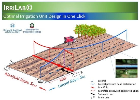
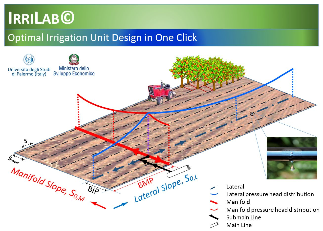
IRRILAB software application introduced by Baiamonte [29] allows a simple design of micro-irrigation units and can be applied to any laterals and manifold slopes. IRRILAB requires a simple rectangular sketch, oriented any way in the space, and defined by two slope values, one for the laterals and one for the manifold. By considering the possible combinations of: (1) horizontal, downward, or upward sloped laterals and manifold, (2) the manifold position with respect to the laterals (BMP = 0, 0.24, or 0.5), and (3) the best inlet position with respect to the manifold (BIP = 0, 0.24, or 0.5), IRRILAB accounts for 25 irrigation unit layouts, as shown in Figure 1, providing for each of them the maximum energy-saving and water use efficiency.

For each layout, the derived explicit relationships can be gainfully used to further derive other design parameters, such as the emitter’s hydraulic characteristics, the required inlet flow rate, the inlet pressure head, the manifold inside diameter, the number of rows, the irrigation unit area, and the water application rate, as well as other important variables such as the Reynolds number for laterals and manifold [29].

The first IRRILAB validation in the field was performed for Layout #17, which is marked by green color in Figure 1, through accomplished work of a Master of Science thesis at the University of Palermo [33]. The pressure distribution was checked in field experiments for a rectangular sector uniform in slope, for both manifold and laterals, and compared with those obtained by IRRILAB. This experimental validation showed very promising results since data provided by IRRILAB matched the experimental ones.

2.2. IRRIPRO Software

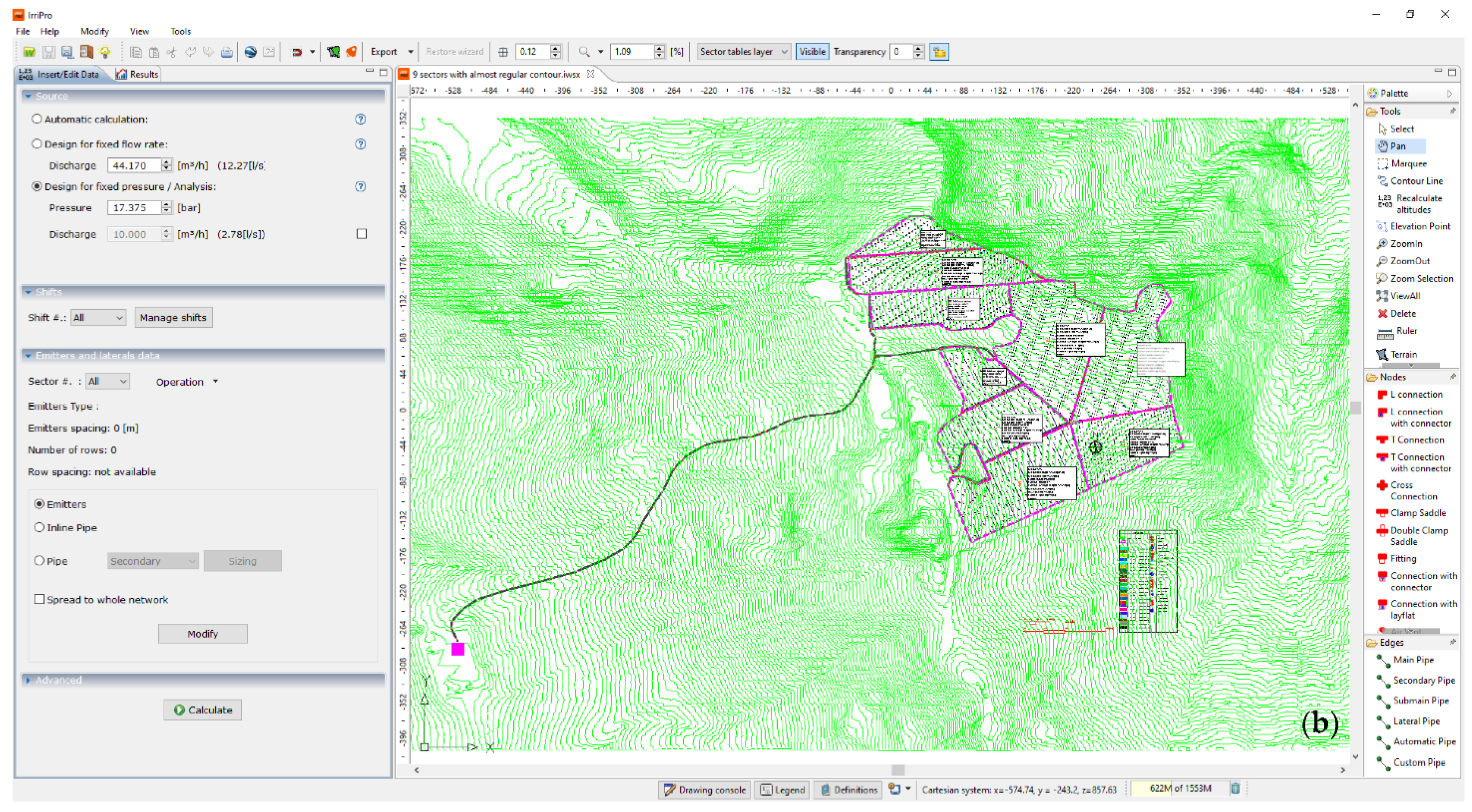
IRRIPRO software represents an innovative and powerful product based on an innovative algorithm that makes it possible to numerically design micro-irrigation subunits with any planform geometry. The proposed algorithm, based on numerical simulations, assures the correct design of the micro-irrigation systems, which enables the design and management. This method provides all the tools for analysis and diagnostics needed to evaluate the effects of each design choice made by the user, the identification of potential malfunctions, and shows a graphical representation of the results, especially in terms of pressure head distribution, which can be easily detected by colored maps, highlighting the overpressure and under-pressure conditions (Figure 2a). In addition, there is the possibility to compare the different design choices with a calculation of the different solutions’ costs, through the detailed database that is included in the software. The materials present in the markets, so the cheapest solution can be adopted, is also considered [27].

IRRIPRO takes into account any planform geometry and slope of the sector and starts from the hydraulic and geometric parameters for achieving the design (Figure 2b). The latter allows the users to easily proceed to input the geometric, topographic, and hydraulic data of the irrigation systems [27].

Arshad et al. [34] mentioned that the results provided by IRRIPRO are considered a good representation of the micro-irrigation system compared to the field results; in addition, the IRRIPRO software can help to test and analyze any alternative design from a hydraulic and economic point of view.

2.3. Motivation of Joint Use of IRRILAB and IRRIPRO

Notwithstanding the many advantages of IRRILAB, which is based on analytical solutions and does not require trial-and-error attempts and iterations, the slope uniformity and the rectangular planform geometry is an important condition to be respected. Moreover, IRRILAB can be applied to just one rectangular unit and does not allow the user to simultaneously design a multiplicity of subunits. It is unlike its counterpart IRRIPRO, which is based on the numerical solutions according to the Step-By-Step (SBS) procedure, and needs many trial-and-error attempts and iterations for solving tedious calculations for designing micro-irrigation units, especially when working with common emitters (CEs) in sloping fields. The latter issue is particularly important, since CEs require the pressure head–flow rate relationship to be considered, whereas pressure compensating emitters (PCEs), which theoretically assumed a constant emitter flow rate, are much simpler to use in sloping fields.

IRRIPRO can design micro-irrigation subunits characterized by non-uniformity slopes and irregularity of the subunit planform geometry. In the meantime, IRRIPRO is lacking the advantages of IRRILAB in saving energy by achieving the allowed pressure head values, and in finding the solution without iterations and attempts. Therefore, the joint use of IRRILAB and IRRIPRO software may offer a unique solution in designing micro-irrigation units, through capturing the positive aspects of both, and meanwhile overcoming the negative ones. Thus, the joint use of both software could lead to design by IRRILAB and verifying the results by IRRIPRO, being much less time-consuming and much more energy-saving.

3. IRRILAB and IRRIPRO Applications

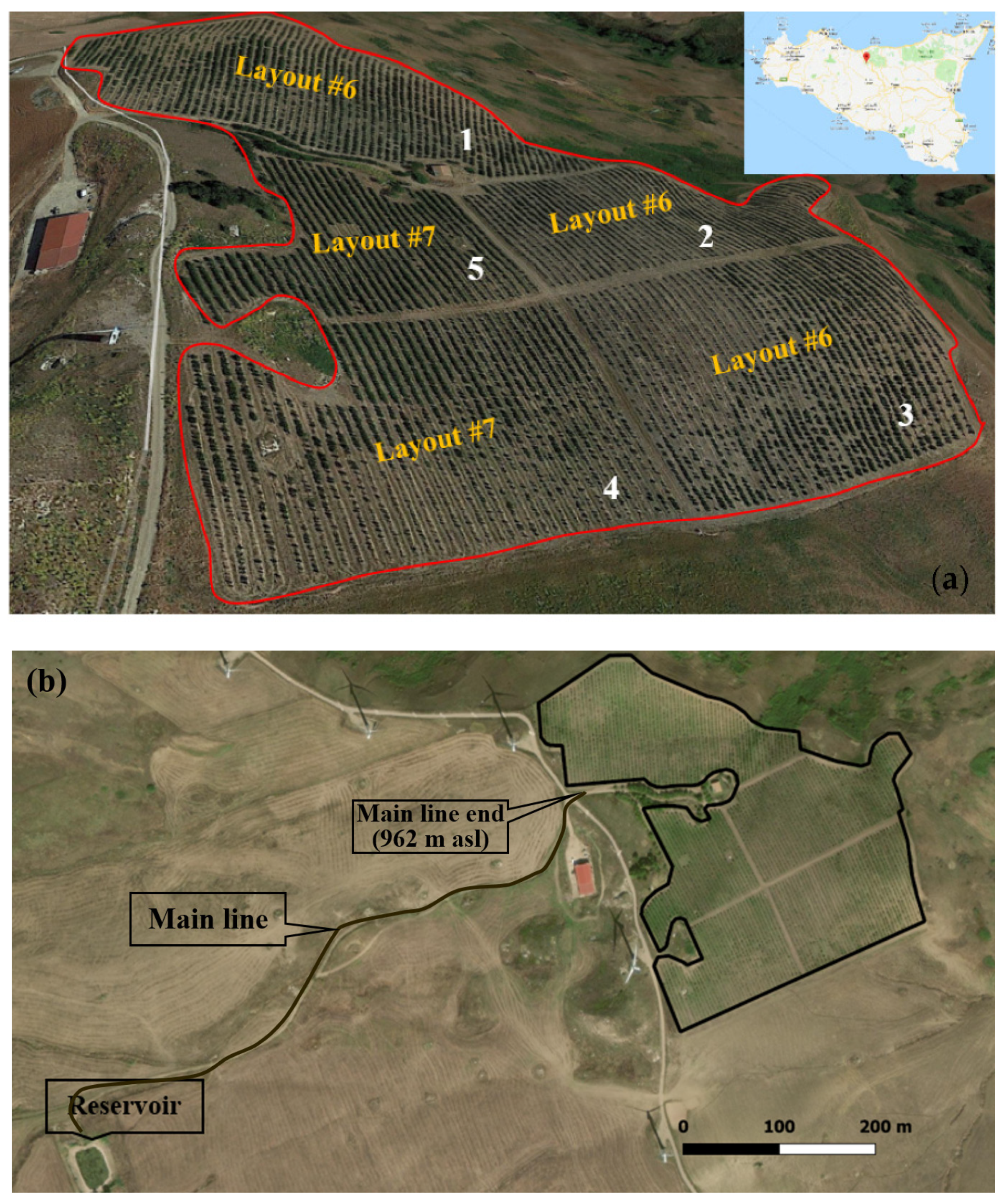
The study area is an apple farm named MELIDIONALE (www.melidionale.it, accessed on 25 September 2020, by Giacomo Armò Pirrone), located at Mangiante, near Caltavuturo (Palermo, Sicily), as displayed in Figure 3a. The MELIDIONALE farm is extended about 8.5 hectares, and it is characterized by a mean altitude of about 950 m a.s.l. The climate is Mediterranean, characterized by abundant rainfall accompanied by snowy phenomena in winter, with an average annual temperature of around 10–17°C. The entire agricultural holding in MELIDIONALE farm is managed in compliance with the re-quire-ments applicable to organic production.

To satisfy the crop water requirement, the farm has a reservoir, with a usable water capacity of 8500 m³, as shown in Figure 3b. The reservoir is located at 103 m below the apple farm (Figure 3b), so a lot of energy is required by the micro-irrigation system, and the farmer is interested in reducing the required energy and increasing the emission uniformity as much as possible.

Actually, the farm is subdivided into five cultivated sectors. These sectors were characterized by “non-uniformity” in the slopes and in the planform geometry, as shown in Figure 3a, which illustrates a three-dimensional (3D) Google Earth view of the actual apple farm, not fitting the IRRILAB requirements enough. Thus, this case study is a good experimental area to test IRRILAB and to show its design performance in case of addressing the issue pertaining to the non-uniform topography, and also to compare IRRILAB results with IRRIPRO standing alone, without IRRILAB suggestions.

Towards this aim, the micro-irrigation system of the actual “non-uniform” five sectors of the farm was designed twice. First by IRRILAB and by using IRRIPRO to verify its design, and second by IRRIPRO, independently of IRRILAB suggestions, i.e., by attempts. Moreover, two different types of emitters (CEs and PCEs) were considered in order to make it possible to compare both emitter types with reference to both software. For verifying the latter in detail, the apple farm was subdivided into sectors as uniform as possible to fit the IRRILAB requirements, as it is described in the next section. Local losses due to the emitters’ insertion into the laterals, which IRRIPRO can consider and in IRRILAB are not implemented yet [35], were neglected in both software to make comparisons homogeneous.

3.1. IRRILAB Applications

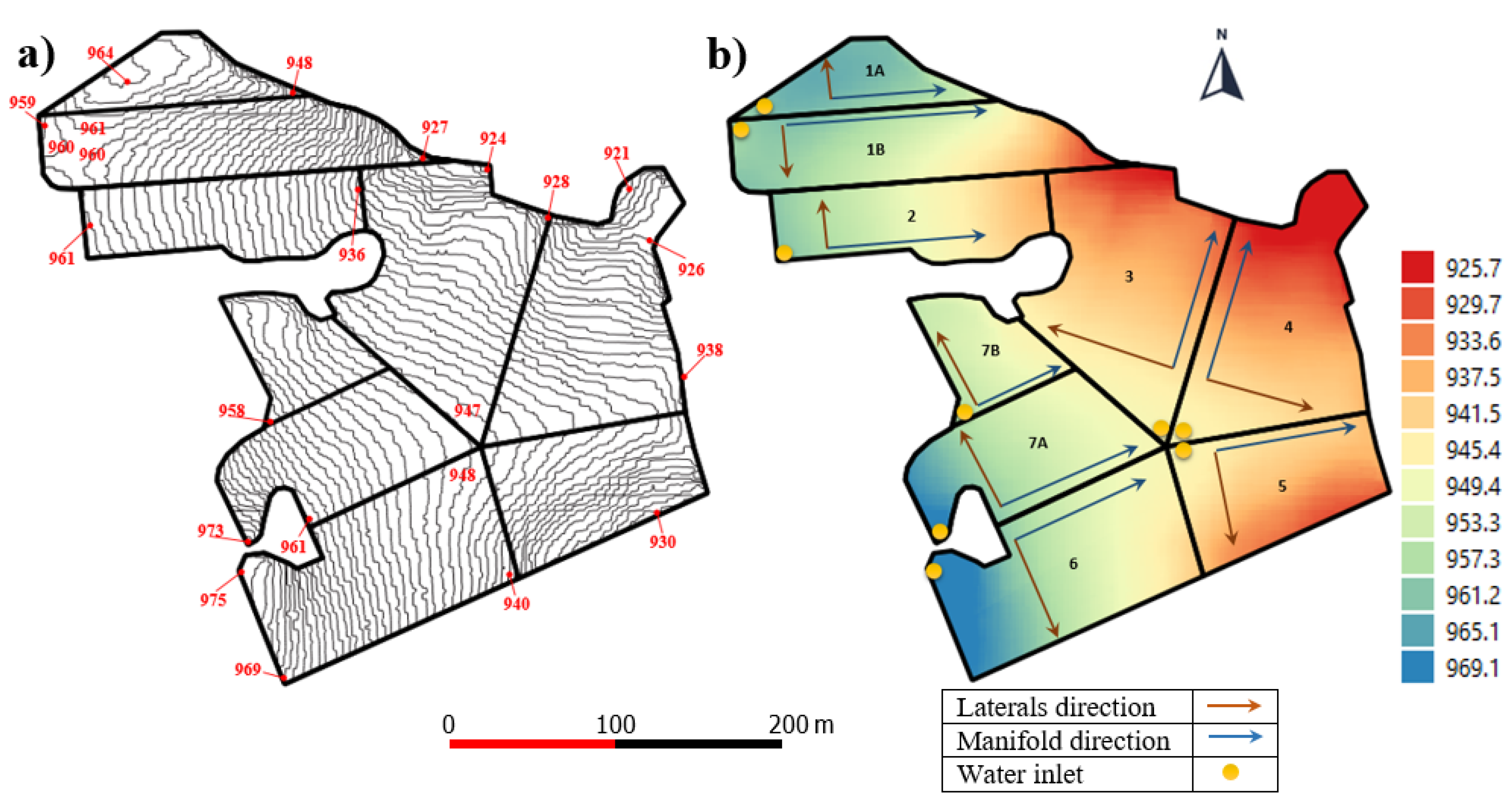
For each sector, the mean slope along the laterals (S_0,L) and manifold (S_0,M) directions, which are sensitive parameters in IRRILAB, were calculated by minimizing the mean square error between the actual elevation distribution of each sector, and that of the equivalent rectangular plane, described by the corresponding plane Equation (1):

$$S_{0,M}x+S_{0,L}y+cz=d$$

(1)

where x, y, and z are the 3D coordinates, d is a parameter that refers to the elevation reference, and c = √ (1 − S_0,L² − S_0,M²). As an example, Figure 4 shows two different 3D views of sector #4 illustrated in Figure 3a. In Figure 4, the red color indicates the actual morphology of sector #4, while the blue color indicates the corresponding equivalent sector with uniform slopes. Figure 4 also shows the vector u (S_0,L, S_0,M, c) normal to the equivalent plane (blue line).

The parameters corresponding to the position of the manifold (BMP) and that of the water inlet into the manifold (BIP) were selected (Figure 1) according to the slopes of the actual 5 sectors, which correspond to Layout #6 (for sectors #1, #2, and #3) and to Layout #7 (for sectors #4 and #5).

After the farm subdivision into a higher number of sectors, as it will be discussed later, Layout #22 was also considered, which together with Layout #6 and #7, mentioned above, are marked by red circles in Figure 1. The sketches of the laterals (L2, L5), which depend on S_0,L and BMP, and those of the manifold (M1, M2), which depend on S_0,M and BIP, are involved in all the considered layouts (#6, #7, and #22), and are illustrated in

Table 1. (a) Lateral’s sketch of the considered lateral layouts L2 and L5, and corresponding coefficients of the nominal emitters’ pressure head and flow rate design relationships, α and α^′, as a function of the calibration constants mentioned in Table 2. Rearranged with permission from ref. [29], Copyright 2020, Elsevier (Amsterdam, The Netherlands); (b) Manifold’s sketch, of the considered manifold layouts M1 and M2. Rearranged with permission from ref. [29], Copyright 2020, Elsevier (Amsterdam, The Netherlands).

(a)
Lateral Layout (Figure 1)	Slope, S0,L	BMP	Lateral’s Sketch	Nominal Pressure Head Coefficient α Equation (1)	Nominal Flow Rate Coefficient α′ Equation (2)
L2	< 0	0		$\frac{1}{\left(1-BMP\right) B_{1,L}}$	$\frac{ B_{2,L}}{ B_{1,L} k_L^{1/r_L}}$
L5	> 0	0		$\frac{1}{BMP B_{1,L}}$	$\frac{ B_{2,L}}{ B_{1,L} k_L^{1/r_L}}$
(b)
Manifold Layout (Figure 1)	Slope, S0,M	BIP	Manifold’s Sketch
M1	< 0	0.24
M2	< 0	0

a,b, respectively (rearranged by Baiamonte [28]). Therefore, as can be seen in these tables, designing each sector by IRRILAB and detecting the corresponding layout requires BMP, BIP, and the sign (negative downward and positive upwards) of the laterals and manifold slopes to be established (S_0,L, S_0,M).

For common emitters (CEs), the IRRILAB design is performed according to the common design procedure that considers a value of the pressure head tolerance, δ = 0.1, in each sector, whereas in the case of using pressure compensating emitters (PCEs), the pressure head tolerance can be set as significantly increased (δ = 60%).

For each layout, other required IRRILAB input are the lateral length, L_opt,L, the lateral inside diameter, D_L, the emitters spacing, (S = 1 m), the laterals spacing, (S_rows = 3.8 m), as well as the pressure head tolerance for both the laterals, δ_L, and the manifold, δ_M. The output data are the design variables, namely the nominal (average) emitter pressure head, h_n, the design emitter flow rate, q_n, the manifold inside diameter, D_M, the number of rows, n_rows, the required inlet flow rate, q_in, and the inlet pressure head, h_in [28].

In IRRILAB, the pressure head tolerance of the irrigation unit, δ, is linked to the laterals pressure head tolerance, δ_L, and to the manifold pressure head tolerance, δ_M, which can be arbitrarily fixed. If one wanted to fix the pressure head tolerance of the irrigation unit (δ = 10%) and that of the lateral δ_L (<0.1), the manifold pressure head tolerance, δ_M, can be calculated by the relationship, δ = (1 + δ_L) (1 + δ_M) − 1, suggested by Baiamonte [28], which yields (Equation(2)):

$${\delta }_M=\frac{1+\delta }{1+{\delta }_L}-1$$

(2)

It should be noticed that, for a fixed δ value, the unit design by IRRILAB output parameters should provide a pressure head distribution in between the theoretical minimum admitted pressure head, h_min = h_n (1 − δ), and the theoretical maximum admitted pressure head, h_max = h_n (1 + δ), only if the planform geometry of the sector is rectangular and the sector is uniform in slope.

The aforementioned consideration explains why the investigated farm, characterized by irregular slopes and planform geometry, was chosen to test, in each sector, the goodness of the IRRILAB design by using its output parameters as input in IRRIPRO. Indeed, for regular sectors, IRRILAB was already fully tested numerically, as can be seen in Figure 4 and in Figure 9 reported in Baiamonte [29].

In IRRILAB, the explicit design relationships that are used vary according to BMP, BIP, S_0,L, and S_0,M, providing the already mentioned 25 layouts (Figure 1). In the following, for the Layouts #6, #7, and #22, which were considered in the present study and that can be solved by using the same design relationships (see layouts #6, #7, and #22 in Table 5 reported in Baiamonte [29]), the IRRILAB procedure is shortly summarized. First, the nominal emitter pressure head, h_n, and the nominal emitter flow rate, q_n, need to be calculated according to [29] Equations (3) and (4):

$$h_n=\alpha \frac{L_{opt,L}\left|S_{0,L}\right|}{{\delta }_L} =\alpha \frac{n_{opt }S \left|S_{0,L}\right|}{{\delta }_L}$$

(3)

$$q_n={\alpha }^{\prime } \frac{D_L^{s_L/r_L}{\left|S_{0,L}\right|}^{\left(1+r_L\right)/r_L} S}{{\delta }_L h_n}$$

(4)

where the optimal lateral length, L_opt,L, could be determined by the known emitter spacing, S, and by the optimal number of emitter, n_opt, r_L and s_L are the flow rate and the inside diameter exponent of the flow resistance equation (Blasius or Hazen-Williams) adopted for the laterals (

Table 2. Resistance equation parameters of the laterals (r_L, s_L, k_L), best manifold position (BMP), and calibration constants (B₁, B₂), for Blasius and Hazen-Williams formula. Rearranged with permission from ref. [29], Copyright 2020, Elsevier (Amsterdam, The Nether-lands).

Resistance Equation	rL	sL	kL	BMP	B1	B2
Blasius	1.750	4.750	7.788 10−4	0.24	7.35	2.34
Hazen-Williams	1.852	4.871	10.675 C−r	0.25	7.07	2.34

), α is the coefficient of nominal pressure head, and α^′ is the coefficient of nominal flow rate (Table 1a) as a function of the calibration constants, B₁, B₂, and BMP, which are also reported in Table 2.

Once the design emitter flow rate and the emitter pressure head are known, for any exponent x of the CE flow rate–pressure head relationship, IRRILAB provides the emitter parameter, k_e, to be chosen:

$$k_e= \frac{q_n}{h_n^x}$$

(5)

To calculate the number of rows, n_rows, which can be installed in the manifold, Baiamonte [28] applied the relationship derived for the laterals to the manifold, considering that a manifold can be seen as a lateral with laterals in place of emitters. Thus, by replacing the lateral pressure head tolerance, δ_L, with the manifold pressure head tolerance, δ_M, the emitter’s spacing, S, with the drip laterals spacing, S_rows, and lateral’s slope, S_0,L, with the manifold slope, S_0,M, the relationship of the number of rows, n_rows, was derived starting from that expressing the number of emitters for the laterals (Equation (3)), yielding:

$$n_{rows}= \beta \frac{\mathsf{\Delta } h_n {\delta }_M}{\left|S_{0,M}\right| S_{rows}}$$

(6)

where β is the number of rows coefficient reported in

Table 3. For layouts #6, #7, and #22, considered in the IRRILAB applications, coefficients of number of rows and manifold inside diameter design relationships, β and β^′, as a function of the calibration constants, which were reported in Table 1. Rearranged with permission from ref. [29], Copyright 2020, Elsevier (Amsterdam, The Netherlands).

Layout	Lateral Layout			Manifold Layout			β	Different Resistance Equation for L and M β′	Same Resistance Equationfor L and M β′
	#	S0,L	BMP	#	S0,M	BIP
6	L2	<0	0	M1	<0	0.24	$B_{1,M}$	$k_1 {\left( B^{*}\left(1-BMP\right)B_{1,L}\right)}^{\raisebox{1ex}{$r_M$}\!\left/ \!\raisebox{-1ex}{$s_M$}\right.}$	${\left( \left(1-BMP\right) B_1\right)}^{\raisebox{1ex}{$r$}\!\left/ \!\raisebox{-1ex}{$s$}\right.}$
7	L2	<0		M2	<0	0	$\left(1-BIP\right) B_{1,M}$	$k_1 {\left(B^{*}\left(1-BMP\right)B_{1,L}\right)}^{\raisebox{1ex}{$r_M$}\!\left/ \!\raisebox{-1ex}{$s_M$}\right.}$	${\left( \left(1-BMP\right) B_1\right)}^{\raisebox{1ex}{$r$}\!\left/ \!\raisebox{-1ex}{$s$}\right.}$
22	L5	>0		M2	<0		$\left(1-BIP\right) B_{1,M}$	$k_1 {\left( B^{*}BMP B_{1,L}\right)}^{\raisebox{1ex}{$r_M$}\!\left/ \!\raisebox{-1ex}{$s_M$}\right.}$	${\left(BMP{B}_1\right)}^{\raisebox{1ex}{$r$}\!\left/ \!\raisebox{-1ex}{$s$}\right.}$

, as a function of the calibration constants, B₁ and BIP. The symbol $\mathsf{\Delta }=1+{\delta }_L$ indicates an amplification factor for the manifold pressure tolerance, that for the manifold, contrarily to the laterals where the pressure head tolerance has to be referred to the design pressure, h_n, it has to be referred to the maximum pressure achieved in the laterals, h_M = h_n (1 + δ_L).

The manifold inside diameter, D_M, is calculated by considering that the flow rate of each lateral can be obtained by multiplying the emitter flow rate, q_n, with the optimal number of emitters, n_opt [28]:

$$n_{opt} q_n= {{\alpha }^{\prime }}_M\frac{D_M^{s_M/r_M} {\left|S_{0,M}\right|}_{.}^{\left(1+r_M\right)/r_M} S_{rows}}{{\delta }_M h_n}$$

(7)

where α^′_M corresponds to the α^′ coefficient of Table 1a, referred to the manifold calibrations constants (B_1,M, B_2,M) and to the manifold resistance equation coefficients (k_M, r_M, Table 2). By substituting Equation (4) into Equation (7), Baiamonte [29] derived an explicit and compact relationship of the inside manifold diameter, D_M:

$$D_M = {\beta }^{\prime } D_L^{\frac{r_M}{r_L}\frac{s_L}{s_M}}{\left(\frac{h_n {\delta }_M \mathsf{\Delta } }{S_{rows} }\frac{S_{0,L}^{1/r_L} }{S_{0,M}^{1+1/r_M} }\right)}^{\frac{r_M}{s_M}}$$

(8)

where β^′ is the manifold inside diameter coefficient (Table 3), as a function of BMP, r_M, s_M, and the numerical constant reported in Table 2.

However, the aforementioned procedure to calculate n_rows and D_M can only be applied for a new irrigation unit, where any possible number of laterals can be installed in a manifold (Equation (6)). For the applications performed here, where IRRILAB is applied to an already designed irrigation system, so that the number of rows is imposed, the IRRILAB explicit relationships need to be reformulated, since the emitters’ characteristics (x, k_e) that match n_rows are required, because in this case, n_rows is an imposed parameter.

By fixing the exponent x, the k_e coefficient of the emitter can be derived by combining Equations (3)–(5), which provides the following k_e relationship:

$$k_e=\frac{{\alpha }^{\prime }}{{\alpha }^{1+x}} \frac{D_L^{s_L/r_L}{S}^x {\delta }_L^x}{ n_{opt}^{1+x} {\left|S_{0,L}\right|}^{x-1/r_L}}$$

(9)

Equation (9) could be applied just for one-lateral units, since no constraints referred to the manifold are imposed yet. Towards this aim, for any imposed number of rows, n_rows, the corresponding manifold pressure head tolerance, δ_M, can be derived by Equation (6):

$${\delta }_M=\frac{n_{rows }{S}_{0,M} S_{rows}}{\beta \mathsf{\Delta } h_n}$$

(10)

By inserting Equation (3) into Equation (10), gives:

$${\delta }_M=\frac{n_{rows } S_{rows} {\delta }_L}{\alpha \beta \left(1+{\delta }_L\right) n_{opt }S}\frac{S_{0,M}}{S_{0,L}}$$

(11)

Equation (11) cannot be solved alone, since according to the IRRILAB design, δ_M also has to satisfy Equation (2). Thus, by imposing Equations (2) and (11) as equal, an explicit relationship of the lateral pressure head tolerance, δ_L, can be derived:

$${\delta }_L=\frac{\alpha \beta \delta n_{opt } S S_{0,L}}{\alpha \beta n_{opt } S S_{0,L}+n_{rows} S_{0,M} S_{rows}}$$

(12)

Interestingly, for a fixed sector geometry, Equation (12) only depends on the unit pressure tolerance, δ, and does not depend on D_M. Equation (12) can be usefully substituted into Equation (9) to derive the emitter’s characteristic k_e that needs to be set, for a fixed x, when the number of rows, n_rows, is assigned:

$$k_e= \frac{{\alpha }^{\prime } D_L^{s_L/r_L}{S}^x }{{\alpha }^{1+x} n_{opt}^{1+x} {\left|S_{0,L}\right|}^{x-1/r_L}}{\left(\frac{\alpha \beta \delta n_{opt } S S_{0,L}}{\alpha \beta n_{opt } S S_{0,L}+n_{rows} S_{0,M} S_{rows}}\right)}^x$$

(13)

Equation (13), which does not depend on D_M, as Equation (12), helps with detecting the optimal emitter’s characteristics (k_e, x) for a fixed n_rows and can be used for both CE and PCE emitters. Indeed, for PCE, that is when x = 0, Equation (13) reduces to:

$$k_e= \frac{{\alpha }^{\prime } D_L^{s_L/r_L} {\left|S_{0,L}\right|}^{1/r_L}}{\alpha n_{opt} }$$

(14)

In conclusion, Equations (13) and (14) can be used for the purpose of this study, since they make it possible, for a fixed sector geometry (n_opt, n_rows, S_0,L, S_0,M) and drip laterals diameter (D_L), to determine the emitter’s characteristic k_e, for CE and PCE, respectively. Of course, the manifold diameter, D_M, then needs calculating by Equation (8).

3.2. IRRIPRO Applications

First, in order to check IRRILAB results, IRRIPRO was applied by using the same design parameters that were obtained by IRRILAB. Then, IRRIPRO features were used to control the pressure head value in the source, Q_s (see the reservoir in Figure 3b), that makes it possible to impose the inlet pressure head provided by IRRILAB (h_in = Δh_n(1 + δ_M)) at the inlet of each sector.

Thus, the output data by IRRIPRO is considered as a good representation for the IRRILAB design, which can be checked by IRRIPRO that is able to provide emitters’ pressure head distribution illustrated by color maps, indicating the over- and under-pressure conditions. The latter are also supported by the emission uniformity, EU, by the minimum and maximum emitters’ pressure head achieved in each sector, h_min and h_max, in addition to other useful output parameters that will be discussed later.

IRRIPRO software was also applied by a different user than that of IRRILAB, thus independently by IRRILAB suggestions, i.e., by attempts, in order to compare the IRRIPRO stand-alone performance with that obtained by the IRRILAB data, and for both CE and PCE. Moreover, the joint software application made it possible to show the ability of IRRILAB in saving energy through calculating the energy required by the irrigation system, differently designed by both software.

4. Results and Discussion

In this section, results aimed at (i) checking the IRRILAB applications by IRRIPRO, (ii) comparing IRRILAB results with those derived by IRRIPRO standing alone applied by attempts, and (iii) comparing the energy consumptions. The section is organized as follows. First, the aforementioned objectives (i) and (ii) are addressed for the actual five-sector subdivision of the farm (Section 4.1). Second, according to the not satisfying results obtained for the actual “non-uniform” five sectors, the farm was subdivided into “almost uniform” seven and nine sectors to better fit the sectors to the regularity degree required by IRRILAB (Section 4.2). Finally, the energy consumptions by using IRRILAB and IRRIPRO with common emitters and pressure compensating emitters are discussed (Section 4.3).

4.1. Results for the Actual “Non-Uniform” Five Sectors

As mentioned above, first, the IRRILAB software was run for the actual “non-uniform” five sectors of the apple farm using CEs. All the already defined geometric and hydraulic design parameters are reported in

Table 4. Geometric and hydraulic design parameters for the actual “non-uniform” five sectors of the apple farm designed by IRRILAB, for common emitters (CE) and pressure compensating emitters (PCE).

Geometric Parameters
Sector	#Layout	BMP	BIP	nrows	Lopt,L (m)	Lopt,M (m)	S0,L		S0,M		CE		PCE
											DL (mm)	DM (mm)	DL (mm)	DM (mm)
1	6	0	0.24	72	88.96	273.6	−0.0210		−0.1202		12.98	39.3	12.98	39.3
2				49	78.49	186.2	−0.0898		−0.1259			45.8		45.8
3				37	99.17	140.6	−0.0747		−0.0586			46.7		46.7
4	7		0	42	90.33	159.6	−0.0540		−0.1799			39.9		39.9
5				37	84.04	140.6	−0.0414		−0.1566			37.1		37.1
Hydraulic parameters for common emitters (CE) with x = 0.5
Sector	δ	δL	δM	ke	hn (m)	qn (L/h)	hin (m)	hmin (m)	hmean (m)	hmax (m)	Qs (m3/h)	hs (m)	CV	EU (%)
1	0.06	0.004	0.056	0.400	80.2	3.58	85.0	73.2	84.7	102.3	22.98	196.7	3.23	89.2
2	0.08	0.023	0.056	1.247	55.7	9.30	60.1	49.7	55.8	71.1	34.45	157.3	4.21	89.4
3	0.05	0.027	0.022	0.947	49.0	6.63	51.4	41.9	47.2	58.8	23.12	145.3	3.60	89.9
4	0.10	0.015	0.084	0.779	60.2	6.04	66.2	49.1	54.5	70.0	21.15	189.9	4.71	89.3
5	0.09	0.012	0.077	0.784	50.7	5.58	55.3	43.2	49.0	58.8	16.11	176.0	3.59	89.7
Hydraulic parameters for pressure compensating emitters (PCE) with x = 0
Sector	δ	δL	δM	ke	hn (m)	hin (m)		hmin (m)	hmean (m)	hmax (m)	Qs (m3/h)	hs (m)	CV	EU (%)
1	0.425	0.030	0.384	3.578	11.3	16.1		5.1	16.6	34.9	22.35	128.2	0	100
2	0.342	0.097	0.223	9.301	13.0	17.5		6.3	13.3	29.4	34.42	115.4
3	0.168	0.091	0.071	6.627	14.6	17.0		6.9	12.6	24.4	23.56	111.2
4	0.26	0.038	0.214	6.044	23.1	29.2		7.4	13.7	33.3	22.26	155.9
5	0.29	0.040	0.241	5.582	15.7	20.3		6.2	12.9	23.9	16.39	142.5

, together with the emission uniformity, EU, calculated according to Keller and Karmeli [25], and the variation coefficient of pressure head, CV [36].

A commercial inside lateral diameter, D_L = 12.98 mm, was chosen for the laterals, which are characterized by the exponent x = 0.5 for CEs (Equation (5)) and by x = 0 for PCEs.

Applications made by IRRILAB for the imposed pressure head tolerance commonly considered, δ = 0.1 for CE, δ = 0.6 for PCE, did not provided satisfying results (EU < 90%). Only for sector #4 (Figure 3a), which is characterized by a good regularity (as can also be seen by the corresponding contour lines later discussed), did δ = 0.1 provide a satisfying EU value (89.3). Thus, for the other sectors, δ was reduced and after few attempts, and EU almost equal to 90% was achieved, as can be seen in Table 4.

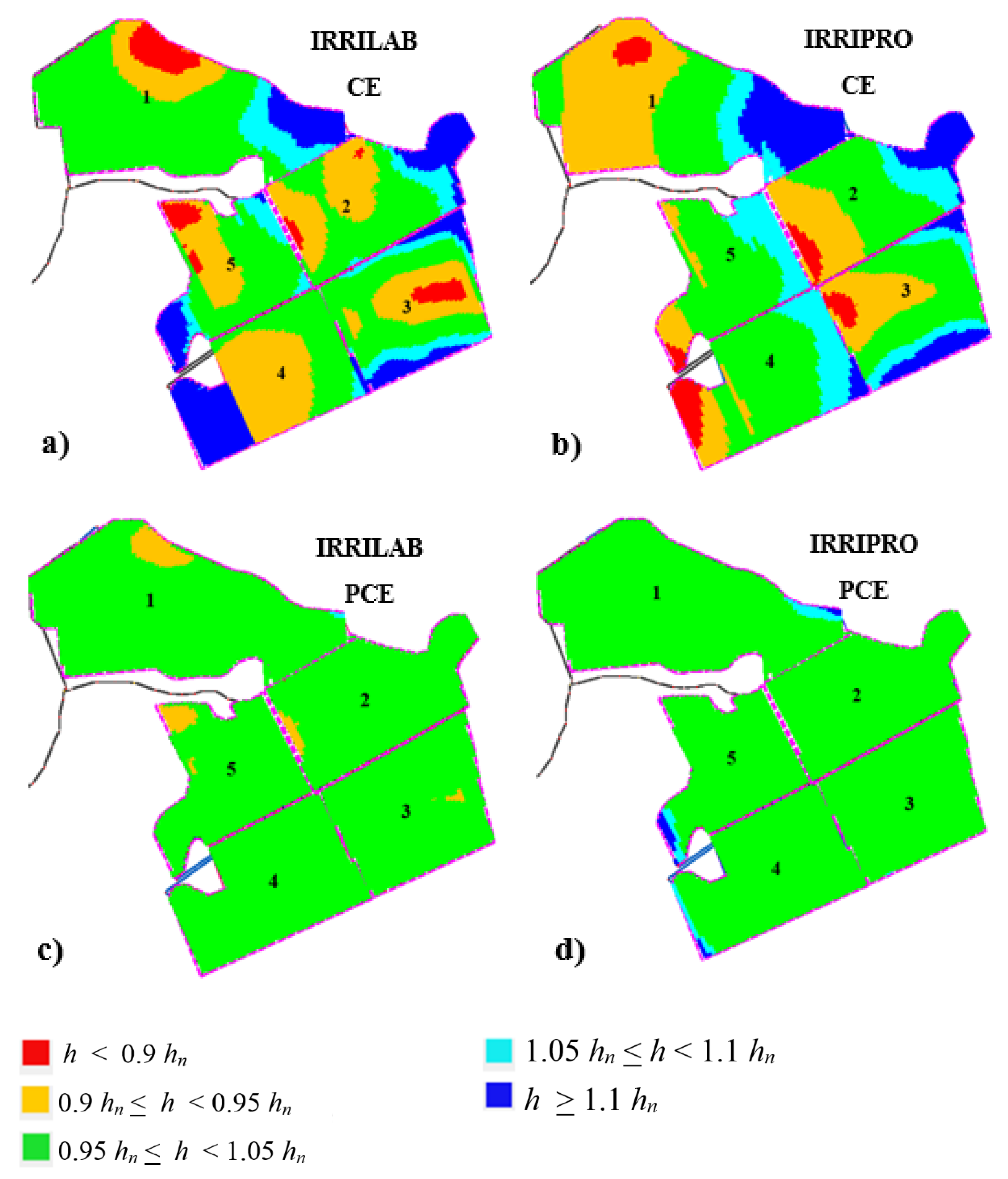
Figure 5a illustrates the results of the emitters’ pressure head distribution map for the whole farm that was obtained by IRRIPRO, using the IRRILAB design parameters. For the actual five sectors of the farm, Figure 5a shows that IRRILAB, from a pressure head distribution point of view, was almost satisfying, since only few areas are in overpressure (h > 1.1 h_n) and in under-pressure (h < 0.9 h_n). This is probably because the actual five sectors did not fully fit the sectors regularity that IRRILAB requires.

The latter consideration is supported by Table 4, where EU ≅ 90% were achieved. More importantly, reducing the pressure head tolerances (δ < 0.1), because of a not too high uniformity of the sectors, determined an increase in the required inlet pressure head and in the corresponding energy required, as can be observed by the high inlet pressure heads, especially for sector #1 that is unreliable (102.3 m).

Contrarily, for sectors #4, #5, and #2, which are characterized by a more sector uniformity, Table 4 shows that an acceptable emission uniformity, EU, almost equal to 90%, can be achieved by only a slight δ reduction. According to these results, it is noteworthy to observe that the more regular the sectors are, the less the δ reduction will be. This IRRILAB behavior will be better described in the next section where the farm will be subdivided into a higher number of sectors.

By applying IRRIPRO, independently of IRRILAB suggestions, by changing the manifold diameter, the emitter flow rate, and inlet pressure, a lot of attempts were necessary to achieve a satisfying emission uniformity, EU. By also using CE, Figure 5b illustrates the best results of emitters’ pressure head distribution designed by IRRIPRO for the actual “non-uniform” five sectors, as in Figure 5a.

For the five sectors and for CEs,

Table 5. Geometric and hydraulic design parameters for the actual “non-uniform” five sectors of the apple farm, designed by IRRIPRO, for common emitters (CE) and pressure compensating emitters (PCE).

Geometric Parameters
Sector	Area (m2)	nrows	LL (m)	LM (m)	S0,L		S0,M	CE		PCE
								DL (mm)	DM (mm)	DL (mm)	DM (mm)
1	24,339	72	87.3	328.3	−0.0210		−0.1202	17.8	78.0	12.98	41.6
2	14,616	49	75.8	213.5	−0.0898		−0.1259				38.0
3	13,944	37	96.3	139.4	−0.0747		−0.0586				38.0
4	14,416	42	87.9	263.2	−0.0540		−0.1799				41.6
5	11,815	37	79.6	152.5	−0.0414		−0.1566				38.0
Hydraulic parameters (CE)
Sector	ke	x	qn (L/h)	Qs (m3/h)	hs (m)	hin (m)	hmin (m)	hmean (m)	hmax (m)	CV	EU (%)
1	1.253	0.5	12.87	80.36	239.6	100.2	94.2	105.6	131.6	4.33	89.3
2	1.253	0.5	11.71	43.33	183.6	82.4	77.4	87.4	105	3.79	89.6
3	1.253	0.5	9.04	32.12	146.8	49.8	46.2	52.1	62.1	3.57	89.9
4	1.253	0.5	12.32	45.39	219.2	84.5	84.3	96.8	115.3	2.97	89.8
5	1.253	0.5	12.46	36.59	213.1	84.8	85.1	98.9	108.9	2.45	89.9
Hydraulic parameters (PCE)
Sector	ke	x	Qs (m3/h)		hs (m)	hin (m)	hmin (m)	hmean (m)	hmax (m)	CV	EU (%)
1	5	0	31.23		140.7	25.7	9.1	20.6	37.2	0	100
2	7		25.91		113.7	19.2	9.1	14.6	25.8
3	7		24.89		126.2	31.4	9.1	19.7	33.8
4	7		25.78		163.6	34.8	9.1	16.2	38.3
5	7		20.56		159.6	35.6	9.1	18.6	38.5

reports the geometric parameters used in IRRIPRO, where it can be observed that the lateral and manifold lengths of IRRIPRO differ from those of IRRILAB. Indeed, for each sector, an equivalent rectangular area equal to the actual one was imposed in IRRILAB. Table 5 also reports the corresponding input and output hydraulic parameters, and shows that the results obtained by IRRIPRO, without IRRILAB suggestions, require a higher pressure at the source, h_s, than those that IRRILAB provided without attempts, which may affect the required energy [37].

Moreover, after a high number of attempts made by a different user compared to that of IRRILAB, it was found that the lateral diameter needed to be increased (D_L = 17.8 mm rather than D_L = 12.98 mm) to find the design solutions, because for the attempts the user made for D_L = 12.98 mm, and by fixing different tentative D_M, the IRRIPRO algorithm did not converge. This is because the IRRIPRO procedure does not include a D_M calculus as IRRILAB does (Equation (8)).

In Figure 5c,d, the pressure head distribution maps corresponding to IRRILAB and IRRIPRO referred to PCEs are illustrated, and the corresponding design parameters are also reported in Table 4 (IRRILAB) and in Table 5 (IRRIPRO). Also, for PCEs, according to non-uniform sector condition, δ was reduced according to the non-uniformity degree, but starting from the mentioned higher value, δ = 60%, than that for CEs (δ = 10%), in order to achieve a satisfying pressure head distribution (Figure 5c,d).

Of course, for PCEs (x = 0, q_n = k_e = constant), the EU value cannot be controlled by IRRIPRO, since EU = 100% (and CV = 0) are imposed (Table 5). In addition, the exponent emitter discharge, x, was assumed as equal to zero, indicating a constant flow rate for the wider range of pressure head. For PCEs, results were satisfying for both IRRILAB and IRRIPRO, in terms of both inlet pressure and pressure head distributions.

Overall, the design of the actual “non-uniform” five sectors of the apple farm using CEs led to reduce the pressure tolerance by 10%, thus high energy consumption would arise, especially for sector #1, which required, for both software, a very high input pressure that is unreliable in practice (85.0 and 100.2 m, respectively). Therefore, the lack of regularity conditions, in both sector slopes and planform geometry, which affected the IRRILAB design, provided not satisfying design results. Contrarily, for PCEs, for both IRRILAB and IRRIPRO, the design solutions are reliable and required low inlet pressure (Table 4 and Table 5). Since this work focused on using CEs, especially for their good durability, a further subdivision aimed at obtaining more regular sectors was performed.

4.2. Subdividing the Apple Farm in Seven and in Nine Sectors

The further subdivision was performed starting from a completely new design and considering the contour lines map and the corresponding digital elevation model (DEM), as illustrated in Figure 6a,b, respectively. At the beginning, the farm was subdivided into seven sectors, which then became nine sectors as a result of splitting sectors #1 and #7 into two subsectors, in order to further fit the IRRILAB requirements as much as possible.

The geometric parameters, corresponding to the seven sectors (1–7) and those to the splitting of sectors #1 and #7, are reported in

Table 6. Geometric and hydraulic design parameters for the apple farm subdivided into seven or nine sectors, by splitting sectors #1 and #7 in two sectors (background gray colored), characterized by an “almost uniform” slope and planform geometry, designed by IRRILAB, for common emitters (CE) and pressure compensating emitters (PCE).

Geometric Parameters
Sector	#Layout	BMP	BIP	nrows	Lopt,L (m)	Lopt,M (m)	S0,L		S0,M		CE		PCE
											DL (mm)	DM (mm)	DL (mm)	DM (mm)
1	7	0	0	63	55.5	239.4	−0.0911		−0.0993		12.98	58.7	12.98	58.7
1A	22			43	23.5	165	0.0429		−0.0610			31.5		31.5
1B	7			63	39.3	239.4	−0.1148		−0.1260			58.6		58.6
2	7			44	45.1	167.2	−0.0203		−0.1476			34.5		34.5
3	22			43	82.3	163.4	0.0351		−0.1463			25.1		25.1
4	7			50	66.8	190	−0.0143		−0.1486			33.5		33.5
5	7			33	65.5	125.4	−0.1639		−0.0918			53.2		53.2
6	7			44	73.6	167.2	−0.0631		−0.1740			42.3		42.3
7	7			40	81.5	152	−0.0335		−0.1503			36.8		36.8
7A	7			39	55.7	148.2	−0.0322		−0.1502			36.2		36.2
7B	7			21	51.7	79.8	−0.0403		−0.1528			30.1		30.1
Hydraulic parameters for common emitters (CE) with x = 0.5
Sector	δ	δL	δM	ke	hn (m)	qn (L/h)	hin (m)	hmin (m)	hmean (m)	hmax (m)	Qs (m3/h)	hs (m)	CV	EU (%)
1	0.04	0.007	0.033	1.167	129.1	13.26	134.2	103.7	116.9	145.9	44.07	243.2	4.01	89.43
1A	0.07	0.017	0.052	1.109	33.7	6.43	36.0	24.6	27.3	39.3	5.46	136.3	4.52	89.51
1B	0.1	0.013	0.086	2.713	62.1	21.38	68.3	51.3	56.8	79.4	47.68	179.3	4.99	89.18
2	0.1	0.004	0.096	1.022	45.8	6.92	50.4	43.1	46.2	54.6	13.01	154.1	2.98	92.88
3	0.1	0.028	0.070	0.213	59.2	1.64	65.1	49.8	54.8	65.6	5.56	153.7	2.57	92.25
4	0.1	0.003	0.096	0.529	52.3	3.83	57.5	43.4	49.0	60.6	12.32	147.0	4.04	89.36
5	0.08	0.039	0.040	2.227	49.8	15.72	53.8	41.8	47.5	56.0	32.88	148.9	3.27	89.95
6	0.1	0.014	0.085	1.043	60.4	8.11	66.5	52.8	57.7	68.5	25.55	187.6	2.71	92.45
7	0.06	0.006	0.053	0.584	76.3	5.10	80.9	63.8	71.0	86.2	15.7	199.1	3.96	90.13
7A	0.1	0.007	0.092	1.111	43.1	7.29	47.4	38.2	42.1	51.6	14.96	164.0	4.08	90.44
7B	0.08	0.012	0.068	1.577	32.0	8.92	34.5	28.1	31.6	37.2	8.92	134.1	3.80	89.86
Hydraulic parameters for pressure compensating emitters (PCE) with x = 0
Sector	δ	δL	δM	ke	hn (m)		hin (m)	hmin (m)	hmean (m)	hmax (m)	Qs (m3/h)	hs (m)	CV	EU (%)
1	0.150	0.026	0.121	13.263	34.4		39.6	5.3	20.3	49.8	46.35	149.9	0	100
1A	0.132	0.032	0.097	6.433	17.9		20.2	7.2	10.2	21.9	6.06	120.5
1B	0.316	0.041	0.264	21.377	19.7		25.9	7.1	13.1	35.8	49.94	138.5
2	0.467	0.017	0.443	6.921	9.8		14.4	7.1	10.3	18.8	12.96	118.2
3	0.337	0.093	0.223	1.638	17.6		23.5	6.8	11.8	23.5	5.78	112.2
4	0.286	0.009	0.274	3.825	18.3		23.5	7.9	13.8	25.4	12.73	113.2
5	0.241	0.116	0.112	15.720	16.5		20.5	6.6	13.6	22.8	33.7	116.3
6	0.368	0.051	0.302	8.108	16.4		22.5	7.0	12.3	24.9	26.16	144.0
7	0.211	0.023	0.184	5.099	21.7		26.3	5.5	13.8	31.7	16.28	144.8
7A	0.323	0.024	0.292	7.295	13.3		17.6	7.1	11.3	22.0	15.16	134.4
7B	0.222	0.032	0.184	8.917	11.5		14.1	7.2	11.0	16.8	8.99	113.7

, where the sectors derived by sector #1 and sector #7 are indicated as sector #1A and #1B, and sector #7A and #7B, respectively (background colored).

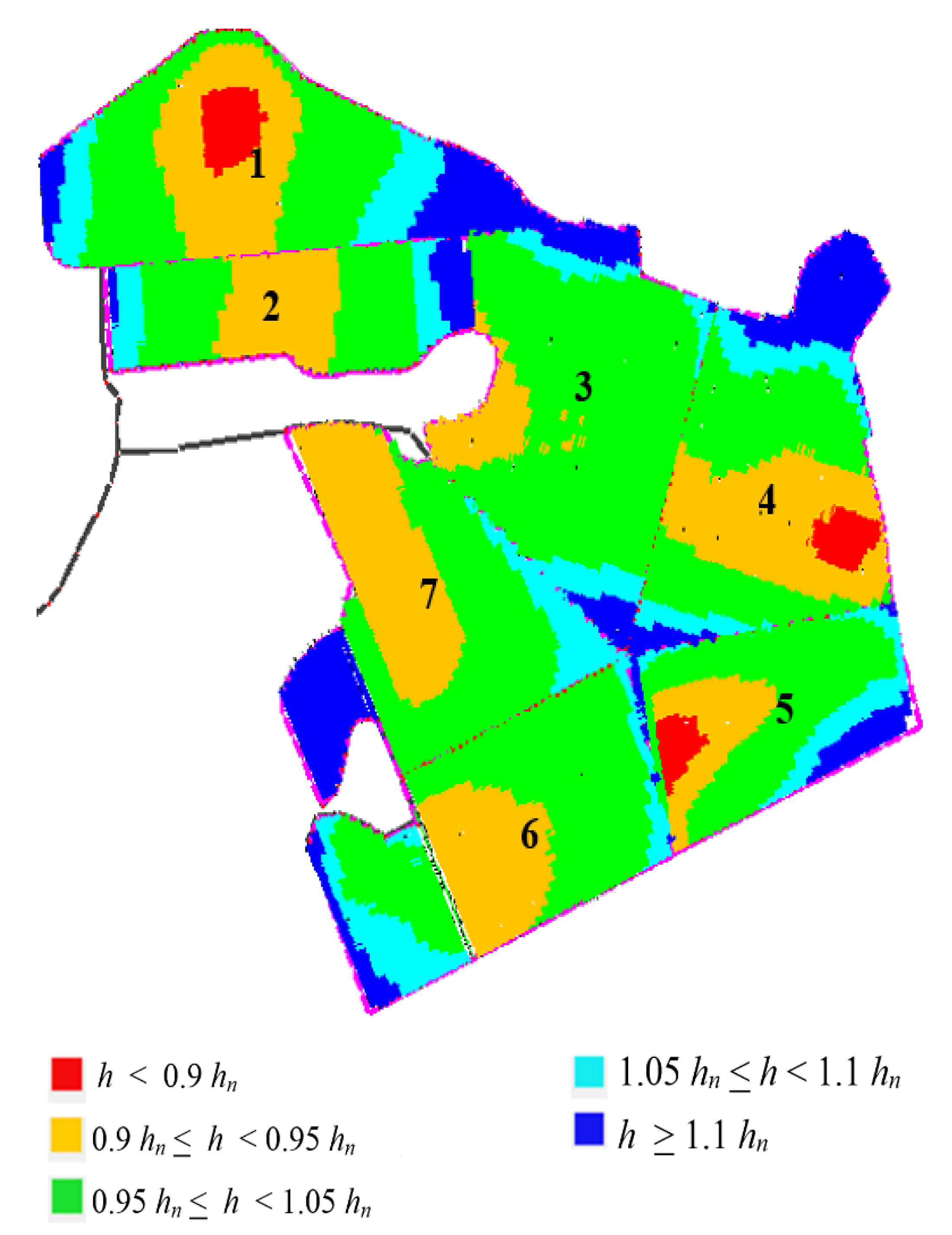
For CEs and for the seven-sector subdivision, results of the hydraulic parameters obtained by IRRILAB are also reported in Table 6 (white background color), whereas the corresponding pressure head distribution map obtained by IRRILAB is illustrated in Figure 7. As can be seen from Table 6 and from Figure 7, the new subdivision improved the IRRILAB results, since for sectors #2, #3, and #6, the optimal design solution (EU ≅ 90%) was immediately found for δ = 0.1, and for sector #5, only a slight δ reduction (δ = 0.08) was needed to achieve EU ≅ 90%. Contrarily, for sectors #1 and #7, which are still characterized by high sectors’ irregularities (in planform geometry and slopes, see Figure 6), the δ reduction necessary to achieve EU ≅ 90% required δ = 0.04 and δ = 0.06, respectively.

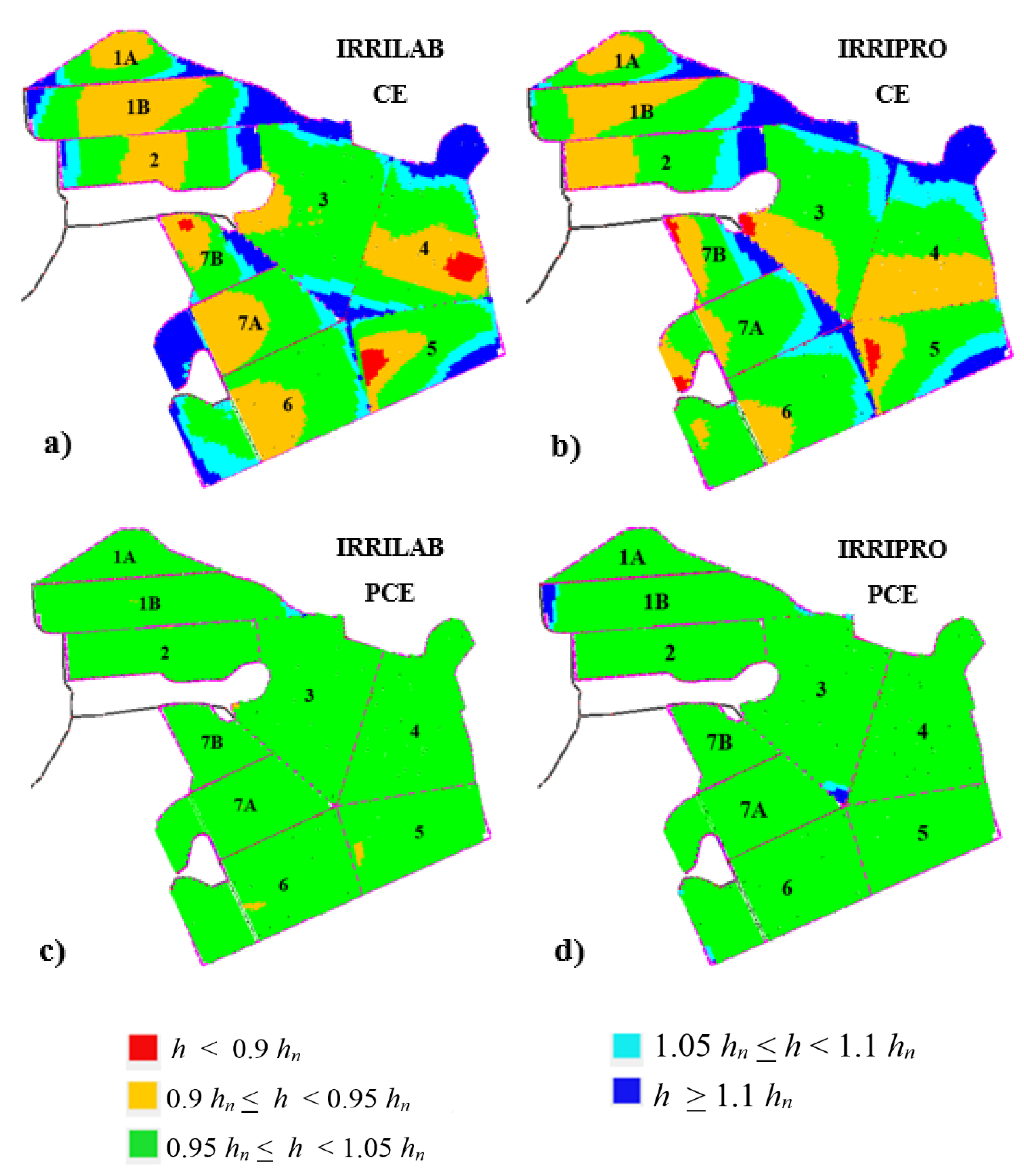
However, again, very high values of inlet pressure heads (134.7 m for sector #1 and 81 m for sector #7) corresponded to this occurrence, which led us to consider these two design solutions unreliable. This is why for sectors #1 and #7, a further subdivision was attempted, with the aim to further investigate the influence of sectors’ irregularities in the IRRILAB design. For CEs, results for the nine-sector subdivision are also reported in Table 6 (background colored for the split sectors #1 and #7), which show that splitting sectors #1 and #7 into two more regular sectors improved the IRRILAB results in terms of both inlet pressure, h_in, and pressure head distribution, as can be observed by comparing sector #1 and sector #7 in Figure 7, with the new sectors #1A, #1B, #7A, and #7b, in Figure 8a.

Similar to Table 6 (for IRRILAB), results derived by IRRIPRO for both seven- and nine-sector subdivision, and for both CE and PCE, are reported in

Table 7. Geometric and hydraulic design parameters for the farm subdivided into nine sectors, by splitting sectors #1 and #7 into two sectors (background colored), characterized by an “almost uniform” slope and planform geometry, designed by IRRIPRO, for common emitters (CE) and pressure compensating emitters (PCE).

Geometric Parameters
Sector	Area (m2)		nrows	LL (m)	LM (m)	S0,L	S0,M	CE		PCE
								DL (mm)	DM (mm)	DL (mm)	DM (mm)
1	13,275		63	55.7	274.8	−0.0911	−0.0993	17.80	78.0	12.98	41.6
1A	3876		43	22.2	159.6	0.0429	−0.0610	12.98	50.0		38.0
1B	9399		63	37.3	248.7	−0.1148	−0.1260	12.98	50.0		38.0
2	7540		44	42.8	170.9	−0.0203	−0.1476	12.98	50.0		38.0
3	13,437		43	82.3	195.3	0.0351	−0.1463	17.80	78.0		41.6
4	12,681		50	66.8	218.9	−0.0143	−0.1486	17.80	78.0		41.6
5	8215		33	65.2	121.2	−0.1639	−0.0918	12.98	78.0		38.0
6	12,282		44	73.6	192.4	−0.0631	−0.1740	12.98	50.0		41.6
7	12,386		40	80.1	187.7	−0.0335	−0.1503	17.80	78.0		41.6
7A	8256		39	53.6	184.1	−0.0322	−0.1502	12.98	50.0		38.0
7B	4129		21	48.3	76.0	−0.0403	−0.1528	12.98	50.0		38.0
Hydraulic parameters (CE)
Sector	ke	x	qn (L/h)	Qs (m3/h)	hs (m)	hin (m)	hmin (m)	hmean (m)	hmax (m)	CV	EU (%)
1	1.253	0.5	11.86	42.49	203.9	95.6	85.0	94.3	122.0	4.12	90.05
1A			7.05	6.64	135.6	35.3	29.0	31.7	44.8	3.99	91.00
1B			10.35	24.18	175.4	72.4	61.5	68.4	90.5	4.26	89.80
2			10.41	19.49	168.3	63.5	63.2	69.0	81.5	3.42	91.60
3			11.14	39.28	173.4	75.7	70.2	79.1	96.3	3.07	90.60
4			11.46	38.15	173.4	76.2	76.0	83.8	100.6	4.00	90.50
5			10.13	21.71	153.0	61.4	57.8	65.4	75.2	3.10	90.40
6			9.89	31.91	188.7	64.9	57.0	62.3	72.3	2.28	92.90
7			11.62	37.09	198.85	74.6	75.1	86.0	96.2	2.81	90.11
7A			9.74	20.24	171.3	53.3	53.3	60.5	68.4	2.59	90.90
7B			9.04	9.11	148.9	49.3	46.2	52.1	59.6	3.55	90.00
Hydraulic parameters (PCE)
Sector	ke		x	Qs (m3/h)	hs (m)	hin (m)	hmin (m)	hmean (m)	hmax (m)	CV	EU (%)
1	5		0	17.48	133.1	32.0	9.1	19.3	43.4	0	100
1A	9			8.48	121.0	20.4	9.1	12.1	24.5
1B	9			21.02	143.5	41.1	9.1	19.4	41.2
2	9			16.86	121.4	17.0	9.1	12.6	21.3
3	7			24.69	131.8	39.2	9.1	19.0	39.2
4	7			23.30	123.5	31.3	9.1	18.4	32.4
5	9			19.30	112.7	21.7	9.1	14.1	23.2
6	9			29.04	157.0	34.3	9.1	15.8	36.0
7	6			19.16	146.6	27.7	9.1	20.4	32.8
7A	9			18.70	142.3	24.6	9.1	14.3	28.6
7B	9			9.07	113.0	13.3	9.1	14.5	21.6

. After a very high number of attempts, IRRIPRO required an increase of the laterals’ diameter for sectors #1, #3, #4, and #7, from D_L = 12.98 to 17.8 mm. Moreover, for sectors #1, #1b, #3, and #4, high values of the inlet pressure heads were achieved, indicating that the results obtained by IRRILAB, without attempts, could be considered more suitable than those obtained by IRRIPRO with attempts, which also required an increase of the laterals’ inside diameter, increasing the material cost. For CEs and for the nine sectors, the corresponding pressure head distributions map derived by the IRRIPRO stand-alone application is reported in Figure 8b.

For both IRRILAB and IRRIPRO, results obtained for PCEs, the case of which however did not require a further subdivision of sectors #1 and #7, are also reported in Table 6 and Table 7, respectively. For IRRILAB, it can be seen that larger pressure tolerances than CEs can be set according to the self-compensating ability of PCEs, which require less inlet pressure heads than CEs. For both IRRILAB and IRRIPRO, pressure head distribution maps corresponding to PCE are reported in Figure 8c,d, which show reasonable results in both cases.

4.3. Evaluating Energy Consumption by Using IRRILAB and IRRIPRO with Common Emitters and Pressure Compensating Emitters

In order to check the IRRILAB goodness of saving energy, for both IRRILAB and IRRIPRO, the energy (E) required for each sector of the actual “non-uniform” five sectors in addition to the “almost uniform” seven and nine sectors were calculated, using the design parameters pertaining to each design, such as the pressure at the source (h_s), the discharge in the source (Q_s), and the nominal emitter flow rate (q_n). Some additional parameters that are necessary for the energy calculus were set as equal in both IRRILAB and IRRIPRO, to make the comparison homogeneous. In particular, the pump and motor drive efficiency (η), the yearly total water application (V), and the years of the irrigation seasons (Y).

The pump power, P (kW), required for each micro-irrigation sector was calculated as:

$$P=\frac{\gamma Q_s h_s}{102 \eta }$$

(15)

where 102 is a conversion factor that makes it possible to express P in (kW), γ is the water-specific weight (1000 kg m⁻³), and Q_s (m³ s⁻¹) and h_s (m) are the discharge and the pressure head at the source. When applying IRRIPRO, h_s was imposed in order to obtain the same inlet pressure head, h_in, provided by IRRILAB, at the inlet of each sector. The pump and motor drive efficiency, η, was fixed at 0.75.

By assuming a yearly total water application V = 200 mm, the yearly time of irrigation, T (h), was calculated according to the emitters’ spacing (S = 1 m) and to the assumed drip lateral spacing (S_rows = 3.8 m):

$$T=\frac{V S S_{rows}}{q_n}$$

(16)

where q_n (L/h) is the emitter flow rate. According to Equations (15) and (16), the total energy consumption, E (kWh), for both IRRILAB and IRRIPRO, when using CEs and PCEs, was calculated as:

$$E=P T Y$$

(17)

The calculated energy required for each irrigation sector designed by IRRILAB and IRRIPRO, with CEs and PCEs, for the subdivision in five, seven, and nine sectors, are reported in

Table 8. Energy, E, required for the micro-irrigation system of the apple farm subdivided in the actual “non-uniform” five sectors, designed by both IRRILAB and IRRIPRO software, for common emitters (CE) and pressure compensating emitters (PCE).

Sector	IRRILAB		IRRIPRO
	E (kWh)		E (kWh)
	CE	PCE	CE	PCE
1	34,866	22,100	41,292	24,249
2	16,074	11,789	18,743	11,611
3	13,991	10,905	14,398	12,386
4	18,342	15,846	22,291	16,624
5	14,021	11,546	17,272	12,938
SUM	97,295	72,187	113,996	77,807

and

Table 9. Energy, E, required for the micro-irrigation system of the apple farm subdivided in the “almost uniform” seven sectors and nine sectors, by splitting sectors #1 and #7 into two sectors (background gray colored), designed by both IRRILAB and IRRIPRO, for common emitters (CE) and pressure compensating emitters (PCE).

Sector	IRRILAB		IRRIPRO
	E (kWh)		E (kWh)
	CE	PCE	CE	PCE
1	22,306	14,456	20,164	12,845
1A	3192	3134	3525	3145
1B	11,037	8928	11,308	9252
2	7994	6107	8693	6276
3	14,401	10,925	16,868	12,829
4	13,070	10,396	15,926	11,344
5	8592	6877	9047	6670
6	16,317	12,824	16,797	13,978
7	16,914	12,758	17,516	12,917
7A	9280	7705	9824	8159
7B	3702	3164	4140	3142
TOTAL 7 sectors	99,594	74,343	105,011	76,859
TOTAL 9 sectors	87,585	70,060	96,128	74,795

, respectively. Results showed that as it could be expected, for both IRRILAB and IRRIPRO, and for both CEs and PCEs, when subdividing the farm into nine sectors, the energy required was less than that required when the farm was subdivided in seven and in five sectors.

A deeper inspection of the energy consumptions derived by IRRILAB and IRRIPRO applications was possible, as seen in Figure 9a (for five sectors) and Figure 9b (for seven and nine sectors). For CEs, the figures also indicate the change of the laterals’ diameter that was needed when applying IRRIPRO, for all the sectors of the five-sector subdivision, and for sectors #1, #3, #4, and #7, of the seven-sector subdivision.

For each sector, Figure 9 shows the ability of IRRILAB in saving energy, with respect to IRRIPRO, for both CEs and PCEs. Only for sector #1 (when seven sectors are considered) and for CEs (Figure 9b) was the energy required by the irrigation system designed by IRRIPRO less than that by IRRILAB.

In terms of total energy requirement, the energy-saving provided by IRRILAB with respect to IRRIPRO was higher for CEs (−15%, −5%, and −9%, for five-, seven-, and nine-sector subdivision, respectively), than for PCE (−7%, −3%, and −6%). However, it is expected that IRRILAB could provide much higher energy-saving than that determined here by increasing the regular degree of the sectors, i.e., when there is no need to reduce the sector pressure head tolerance, δ. The energy-saving found by using IRRILAB in these applications is supported by the results found in a previous work referring to one-lateral units [37], where it was shown that using the entire pressure head range imposed by the pressure head tolerance unit (i.e., the same principle in which IRRILAB is based) provided an important energy-saving, with respect to the case in which the emitter pressure head does not achieve the minimum and the maximum values, imposed by δ (h_min = h_n (1 − δ) and h_max = h_n (1 + δ)).

It is noteworthy that when the regularity conditions of slopes and planform geometry of the “almost uniform” nine sectors were considered, fitting the IRRILAB requirements as much as possible, the total energy was found lower than that obtained from the actual “non-uniform” five sectors. The latter indicates that IRRILAB software could be recommended because it is easy to use, does not require attempts, and makes it possible to save energy, especially when sectors are almost rectangular and uniform in slopes.

For a complete analysis, other differences in output variables should be analyzed, such as the differences in laterals and manifolds inside diameters. However, the cost analysis, including the investment costs, was beyond the purpose of this study.

Finally, it should be noticed that notwithstanding the amount of energy saved could appear limited, at least in this case study, it needs remarking that the greatest benefit derived was the no attempts requirement of IRRILAB, which makes this software a useful tool for a pre-design of micro-irrigation systems.

5. Conclusions

Recently, the IRRILAB software application based on explicit analytical solutions was introduced as a simple tool to design rectangular and uniform slope irrigation units. Since the latter conditions may be impractical in some cases, a Sicilian apple farm (8.5 ha) was selected to apply IRRILAB with different subdivision stages of the farm in order to fit different degrees of regularity of the sectors. First, the actual five sectors in which the farm was subdivided were considered. Second, the farm was subdivided into seven different sectors, and third, two of the seven sectors were split into two sectors, becoming nine sectors.

IRRILAB was verified by inserting its output data as input in IRRIPRO software application, which provides, according to numerical solutions, the pressure head distribution for any shape and slopes of irrigation units. IRRIPRO was also applied by making, contrarily to IRRILAB, a number of attempts as a stand-alone tool, in order to compare the results between the two software applications. IRRILAB and IRRIPRO applications and their comparisons were also performed by using common emitters (CEs) and pressure compensating emitters (PCEs).

The most important results covered in this study can be summarized as follows:

• The IRRILAB application showed its sensitivity to the planform geometry and to the slope uniformity of the laterals and of the manifold, indicating that the more uniform in slope and the more rectangular the sector is, the better and better the design results (in terms of emission uniformity and energy-saving) will be.
• IRRILAB, which is based on analytical solutions and does not require attempts and the trial-and-error technique, offers a valuable solution in designing a micro-irrigation system using CEs or PCEs, and makes it possible to save energy for both emitter types, especially when sectors are almost rectangular and uniform in slope.
• The energy-saving provided by IRRILAB with respect to IRRIPRO, applied by attempts, resulted higher for CEs (−15% for five sectors and −9% for nine sectors) than for PCEs (−7% for five sectors and −6% for nine sectors). However, in absolute terms, the energy required was greater for five-sector subdivision than for nine-sector subdivision.
• PCEs could be considered a good solution for saving energy in the sloping field, but their contraindications need to be mentioned: they are more expansive, more complicated structurally, and the working mechanism is not clear, which causes difficulty in their research and development. The latter causes their damage in the short term and the increase of the manufacturing variation coefficient can frustrate the benefit found in terms of energy-saving.
• For sloping fields, CEs, usually chosen only for flat fields, should be recommended, if a design procedure such as that suggested by IRRILAB is applied, especially for sectors uniform in slopes and rectangular planform geometry.

References

- Food and Agriculture Organization of the United Nations. The State of the World’s Land and Water Resources: Managing Systems at Risk; Earthscan: London, UK, 2011. Available online: http://www.fao.org/docrep/017/i1688e/i1688e.pdf (accessed on 25 September 2020).
- Food and Agriculture Organization of the United Nations. The Future of Food and Agriculture—Trends and Challenges; Food and Agriculture Organization of the United Nations: Rome, Italy, 2017. Available online: http://www.fao.org/3/i6583e/i6583e.pdf (accessed on 25 September 2020).
- UNESCO World Water Assessment Programme. The United Nations World Water Development Report 2020: Water and Climate Change. Available online: https://unesdoc.unesco.org/ark:/48223/pf0000372985.locale=en (accessed on 17 January 2021).
- Postel, S.L. Water for food production: Will there be enough in 2025? BioScience 1998, 48, 629–637. [Google Scholar] [CrossRef] [Green Version]
- WRG. Charting Our Water Future. Economic Frameworks to Inform Decision-Making; The 2030 Water Resources Group: Rome, Italy, 2009. Available online: https://www.2030wrg.org/wp-content/uploads/2012/06/Charting_Our_Water_Future_Final.pdf (accessed on 27 September 2020).
- Scheierling, S.M.; Treguer, D.O. Enhancing water productivity in irrigated agriculture in the face of water scarcity. Choices 2016, 31, 1–10. [Google Scholar]
- Baiamonte, G. Advances in designing drip irrigation laterals. Agric. Water Manag. 2018, 199, 157–174. [Google Scholar] [CrossRef]
- Hamdy, A.; Ragab, R.; Scarascia Mugnozza, E. Coping with water scarcity: Water saving and increasing water productivity. Irrig. Drain. 2003, 52, 3–20. [Google Scholar] [CrossRef]
- Cullotta, S.; Bagarello, V.; Baiamonte, G.; Gugliuzza, G.; Iovino, M.; La Mela Veca, D.S.; Maetzke, F.; Palmeri, V.; Sferlazza, S. Comparing different methods to determine soil physical quality in a Mediterranean forest and pasture land. Soil Sci. Soc. Am. J. 2016, 80, 1038–1056. [Google Scholar] [CrossRef]
- Bucks, D.A.; Nakayama, F.S.; Warrick, A.W. Principles, practices, and potentialities of trickle (drip) irrigation. Adv. Irrig. 1982, 1, 219–298. [Google Scholar]
- Baiamonte, G.; Crescimanno, G.; Minacapilli, M. Effects of Biochar on Irrigation Management and Water Use Efficiency for Three Different Crops in a Desert Sandy Soil. Sustainability 2020, 12, 7678. [Google Scholar] [CrossRef]
- Tiwari, K.N. Feasibility of drip irrigation under different soil covers in tomato. J. Agric. Eng. 1998, 35, 41–49. [Google Scholar]
- Bralts, V.F.; Driscoll, M.A.; Shayya, W.H.; Cao, L. An expert system for the hydraulic analysis of microirrigation systems. Comput. Electron. Agric. 1993, 9, 275–287. [Google Scholar] [CrossRef]
- Trung, M.C.; Nishiyama, S.; Anyouji, H. Hydraulic design of drip irrigation system by the method of unsteady flow: Example in irregular slope field. Sand Dune Res. 2007, 54, 49–56. [Google Scholar]
- Zhu, D.L.; Wu, P.T.; Merkley, G.P.; Jin, J. Drip irrigation lateral design procedure based on emission uniformity and field microtopography. Irrig. Drain. 2010, 59, 535–546. [Google Scholar] [CrossRef]
- Ju, X.; Wu, P.; Weckler, R.; Zhu, D.; Zhang, L. Simplified method for designing diameter of drip irrigation laterals based on emitter flow variation. Trans. Chin. Soc. Agric. Eng. 2016, 32, 14–20. [Google Scholar]
- Myers, L.E.; Bucks, D.A. Uniform irrigation with low-pressure trickle systems. J. Irrig. Drain. Div. 1972, 98, 341–346. [Google Scholar] [CrossRef]
- Howell, T.A.; Hiler, E.A. Trickle irrigation lateral design. Trans. ASAE 1974, 17, 902–908. [Google Scholar] [CrossRef]
- Wu, I.P.; Gitlin, H.M. Energy gradient line for drip irrigation laterals. J. Irrig. Drain. Div. 1975, 101, 321–326. [Google Scholar] [CrossRef]
- Kang, Y.; Nishiyama, S. Analysis and design of microirrigation laterals. J. Irrig. Drain. Eng. 1996, 122, 75–82. [Google Scholar] [CrossRef]
- Jiang, S.; Kang, Y. Simple method for the design of microirrigation paired laterals. J. Irrig. Drain. Eng. 2010, 136, 271–275. [Google Scholar] [CrossRef]
- Baiamonte, G.; Provenzano, G.; Rallo, G. Analytical approach determining the optimal length of paired drip laterals in uniformly sloped fields. J. Irrig. Drain. Eng. 2015, 141, 04014042. [Google Scholar] [CrossRef] [Green Version]
- Xueliang, J.; Pute, W.; Paul, W.R. Newly-simplified method for hydraulic design of micro-irrigation laterals based on emission uniformity. J. Drain. Irrig. Mach. Eng. 2015, 33, 691–700. [Google Scholar]
- Baiamonte, G. Simple relationships for the optimal design of paired drip laterals on uniform slopes. J. Irrig. Drain. Eng. ASCE 2016, 142, 04015054. [Google Scholar] [CrossRef]
- Keller, J.; Karmeli, D. Trickle irrigation design parameters. Trans. ASAE 1974, 17, 678–684. [Google Scholar] [CrossRef]
- Juana, L.; Losada, A.; Rodrigues-Sinobas, L.; Sanchez, R. Analytical relationships for designing rectangular drip irrigation units. J. Irrig. Drain. Eng. ASCE 2004, 130, 47–59. [Google Scholar] [CrossRef]
- Di Dio, P.; Provenzano, G.; Provenzano, C.; Savona, P. IRRIPRO: A Powerful Software to Graphic and Hydraulic Design of Irrigation Plants. In Proceedings of the International Conference on Agricultural and Biosystem Engineering for a Sustainable world, Crete, Greece, 23–25 June 2008; Curran Associates, Inc.: Red Hook, NY, USA, 2008; Volume 1, pp. 1–14. [Google Scholar]
- García, I.F.; Montesinos, P.; Poyato, E.C.; Díaz, J.R. Energy cost optimization in pressurized irrigation networks. Irrig. Sci. 2016, 34, 1–13. [Google Scholar] [CrossRef]
- Baiamonte, G. Explicit relationships for optimal designing rectangular microirrigation units on uniform slopes: The IRRILAB software application. Comput. Electron. Agric. 2018, 153, 151–168. [Google Scholar] [CrossRef]
- Zayani, K.; Alouini, A.; Lebdi, F.; Lamaddalena, N. Design of drip irrigationsystems using the energy drop ratio approach. Trans. ASAE 2001, 44, 1127–1133. [Google Scholar] [CrossRef]
- Wu, I.P. An assessment of hydraulic design of micro-irrigation systems. Agric. Water Manag. 1997, 32, 275–284. [Google Scholar] [CrossRef]
- Vallesquino, P.; Luque-Escamilla, P.L. Equivalent friction factor method for hydraulic calculation in irrigation laterals. J. Irrig. Drain. Eng. ASCE 2002, 128, 278–286. [Google Scholar] [CrossRef]
- Baiamonte, G.; Mangiapane, G. Il software IRRILAB per gli impianti microirrigui: Verifiche numeriche e sperimentali. Conference Proceeding “Attualità dell’idraulica Agraria e delle Sistemazioni Idraulico-Forestali al cambiare dei tempi”, Dipartimento di Scienze Agrarie e Forestali, Palermo. Quad. di Idron. Mont. 2018, 35, 209–218. [Google Scholar]
- Arshad, I.; Savona, P.; Khan, Z.A. Analysis of Trickle/Drip Irrigation Uniformity by IRRIPRO Simulations. Int. J. Res. 2014, 1, 635–649. [Google Scholar]
- Baiamonte, G. Linking kinetic energy fraction and equivalent length method to determine local losses in trickle irrigation. J. Irrig. Drain. Eng. ASCE 2020, 146, 04020024. [Google Scholar] [CrossRef]
- Keller, J.; Bliesner, R.D. Sprinkle and Trickle Irrigation; Van Nostrand Reinhod: New York, NY, USA, 1990. [Google Scholar]
- Baiamonte, G. Minor Losses and Best Manifold Position in the Optimal Design of Paired Sloped Drip Laterals. Irrig. Drain. 2018, 67, 893–908. [Google Scholar] [CrossRef]
Figure 1.
25 irrigation sector layouts considered by IRRILAB, by varying the lateral slope (S0,L < 0, S0,L > 0, S0,L = 0), the best manifold position (BMP = 0, 0.24, 0.5), the manifold slope (S0,M < 0, S0,M > 0, S0,M = 0), and the best inlet position (BIP = 0, 0.24, 0.5). Qualitative pressure head distribution lines are represented for a lateral and for the manifold. Reprinted with permission from ref. [29], Copyright 2020, Elsevier (Amsterdam, The Netherlands).
Figure 2.
The two main interfaces of IRRIPRO software, (a) the main output data panel, and (b) the main input data panel.
Figure 3.
The MELIDIONALE apple farm (Sicily), (a) three-dimensional (3D) Google Earth view, actually subdivided into five cultivated sectors, and (b) two-dimensional (2D) Google Earth view of the apple farm, illustrating the reservoir location (859 m a.s.l.).
Figure 4.
Two different 3D views of sector #4 belonging to the apple farm subdivided in five sectors (numbered in Figure 3a), and the corresponding equivalent sector (blue color) with uniform slopes (S0,L = −0.054 and S0,M = −0.180).
Figure 5.
Emitters’ pressure head distribution maps, pertaining to the design parameters of IRRILAB (a,c) and IRRIPRO (b,d) software applications, for the actual “non-uniform” five sectors of the apple farm, in case of using common emitters (CE) (a,b) and pressure compensating emitters (PCE) (c,d).
Figure 6.
The apple farm subdivided into nine sectors, illustrating (a) the 1 m contour lines, and (b) the DEM with flow directions for laterals (brown lines) and manifold (blue lines). For each sector, the inlet position (•) is also reported.
Figure 7.
Emitters’ pressure head distribution map, pertaining to the design parameters of IRRILAB, by using common emitters (CEs) for the farm subdivided into seven sectors.
Figure 8.
Emitters’ pressure head distribution maps, pertaining to the design parameters of IRRILAB (a,c) and IRRIPRO (b,d) software applications, for the farm subdivided into nine sectors, in case of using common emitters (CE) (a,b) and pressure compensating emitters (PCE) (c,d).
Figure 9.
Comparison between the energy required by the micro-irrigation sectors with the parameters designed by IRRILAB and with those designed by IRRIPRO, by using common emitters (CE) and pressure compensating emitters (PCE), (a) for the actual five sectors, and (b) for the seven and nine sectors.