Short-Term Response of Chlorophyll a Concentration Due to Intense Wind and Freshwater Peak Episodes in Estuaries: The Case of Fangar Bay (Ebro Delta)

Abstract

Estuaries and coastal bays are areas of large spatio-temporal variability in physical and biological variables due to environmental factors such as local wind, light availability, freshwater inputs or tides. This study focuses on the effect of strong wind events and freshwater peaks on short-term chlorophyll a (Chl a) concentration distribution in the small-scale and microtidal, Fangar Bay (Ebro Delta, northwestern Mediterranean). The hydrodynamics of this bay are primarily driven by local wind episodes modulated by stratification in the water column. Results based on field-campaign observations and Sentinel-2 images revealed that intense wind episodes from both NW (offshore) and NE-E (onshore) caused an increase in the concentration of surface Chl a. The mechanisms responsible were horizontal mixing and the bottom resuspension (also linked to the breakage of the stratification) that presumably resuspended Chl a containing biomass (i.e., micropyhtobentos) and/or incorporated nutrients into the water column. On the other hand, sea-breeze was not capable of breaking up the stratification, so the chlorophyll a concentration did not change significantly during these episodes. It was concluded that the mixing produced by the strong winds favoured an accumulation of Chl a concentration, while the stratification that causes a positive estuarine circulation reduced this accumulation. However, the spatial-temporal variability of the Chl a concentration in small-scale estuaries and coastal bays is quite complex due to the many factors involved and deserve further intensive field campaigns and additional numerical modelling efforts.

1. Introduction

Estuaries and bays with intensive shellfish activity require substantial knowledge on the distribution and concentration of phytoplankton for proper management of production, including the growth and harvesting cycles and eventual relocation strategies. In this sense, the biological habitat and the ecosystem characteristics are highly influenced by physical and morphologic dynamics. Estuaries and coastal environments are characterised by complex hydrodynamics with high temporal variability in water circulation due to the joint effect of wind, tides, freshwater inflow, and other episodic events [1,2,3,4,5,6,7,8,9]. In a small-scale, shallow coastal bay (few meters water depth) such as Fangar Bay in the Ebro Delta (NW Mediterranean Sea), the concentration of chlorophyll a (Chl a) shows high variability on a seasonal scale rather than an inter-annual scale [10]. A maximum peak can be observed during the summer and autumn months; from July to November, high concentrations have been observed in comparison to low concentrations during February and May [10]. Spatial variations have also been observed in Fangar Bay, where maximum concentrations were found in the bay mouth and minimum concentrations in the inner bay [11]. However, due to the small-scale and shallowness of the bay, the temporal scale of the dispersion process is small so the concentration of phytoplankton is quickly homogenised [12]. The link between the Chl a concentration and the water circulation has been investigated by Soriano et al. [11], where they explained that the highest concentrations of Chl a occur when the estuarine circulation weakens and decreases after rain events. However, from an episodic event point of view some questions still remain open. For instance, what is the Chl a concentration distribution response to energetic wind episodes? What about in the case of an eventual increase in the freshwater flow?

These seasonal changes in coastal waters have already been addressed. The seasonal cycle of phytoplankton in open waters near the Ebro Delta is characterised (as in other areas of the Mediterranean) by an increase in the Chl a concentration from late autumn, with the weakening and breakdown of the thermocline, culminating in a winter bloom of phytoplankton in January–February [10,13,14]. These seasonal effects within the bay can be associated with biological factors, such as the availability of nutrients due to the entry of freshwater or the activity of filter feeders [10]. In the Ebro Delta bays (i.e., Alfacs at the south hemi-delta and Fangar at the north hemi-delta), the freshwater discharge plays an important role through man-controlled irrigation channels, as well as contributions from aquifers, being an important source of nutrients in coastal areas [15], both inorganic and organic. However, this is not a determining factor since it can happen that when irrigation channels are closed, higher Chl a concentrations are reached in comparison to the open channel period [11]. In consequence, there are many physical and biological processes that can affect the distribution of phytoplankton in coastal waters and estuaries [16,17,18,19] that require intensive field campaigns and large data sets for a robust analysis. The aim of this study was to analyse this distribution in Fangar Bay (as an example of a semi-enclosed environment), focusing on the relationship that can exist between the concentration of Chl a concentration and energetic wind episodes using in situ and satellite data.

The document is organized as follows: Section 2 presents a detailed description of the study area and two field campaigns carried out in Fangar Bay. The collection process of Chl a concentration data (in situ data and the acquisition of satellite images from Sentinel-2) are detailed. Then, Section 3 (Results) presents the Chl a concentration variability according to the different wind episodes, showing both in situ and satellite data. Section 4 discusses the presumable mechanisms of variability in Chl a concentration related to wind-driven currents and the stratification in the water column in the context of the spatio-temporal processes in estuaries and coastal bays. Finally, Section 5 summarizes the main conclusions.

2. Materials and Methods

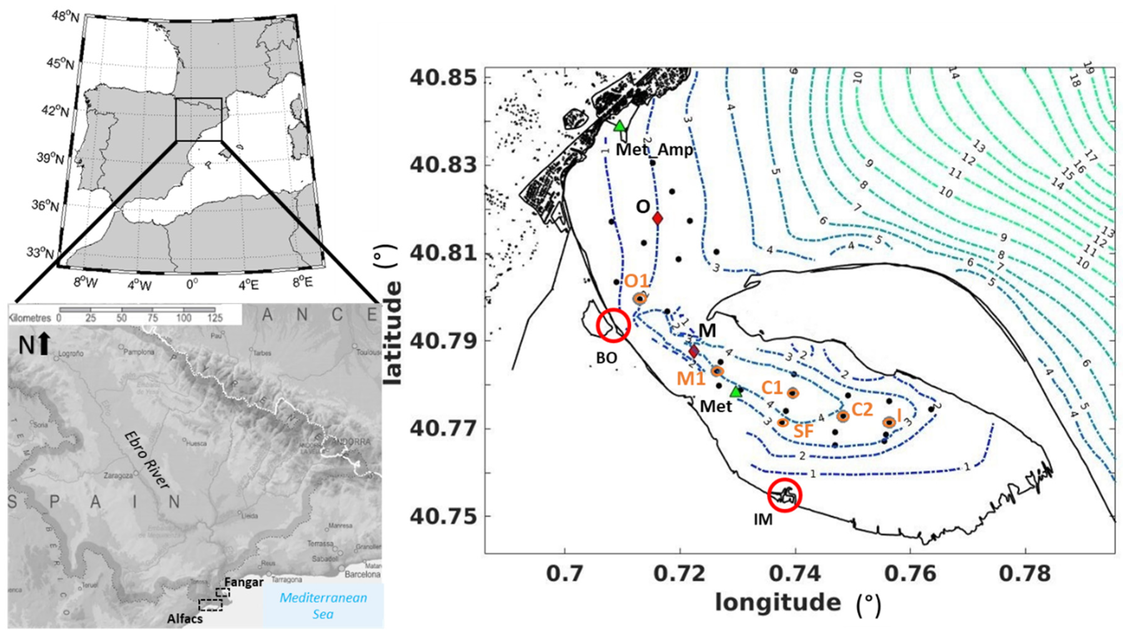
2.1. Study Area

Fangar Bay is part of the Ebro Delta (NW Mediterranean Sea), which extends around 25 km offshore and forms two enclosed bays (Fangar to the north and Alfacs to the south). Both receive freshwater discharges from the irrigation channels of rice fields. The main dimensions of Fangar Bay are 12 km², with a length of about 6 km, a maximum width of 2 km and a volume of water of 16 × 10⁶ m³ [20]. The average depth is 2 m, with a maximum of 4 m (see bathymetry in Figure 1). The connection with the open sea is located in the NW and spans approximately 1 km [21]. In recent years, the mouth width has been modified by the accumulation of sediment from the beach located to the north [22], so its width is currently less than 1 km.

The Fangar area is influenced by the presence of S/SE sea breezes—which do not exceed 6 m·s⁻¹ during the summer and spring seasons—and strong winds from the N and W of more than 12 m·s⁻¹ in autumn and winter [23,24]. The most frequent wind throughout the year is the NW wind, locally known as the Mistral, which is characterised by strong gusts of cold and dry wind [21]. NW winds are associated with general weather patterns and occur throughout the year but have maximal strength and persistence during the cooler months. In addition, the E and NE winds are responsible for rain events and increasing local mean sea level at the coast [25], which can also be quite intense (~10 m·s⁻¹).

The freshwater contribution is regulated by rice cultivation throughout the year. Open channels occur from April to December, receiving a seasonal mean flow of 7.23 m³·s⁻¹ throughout these months [26]. This flow is distributed irregularly throughout the year, with maximum values in the months of April to November. Negligible freshwater flow occurs from December to March when the channels are closed [27]. This flow is distributed in two main freshwater discharges in Fangar Bay: one in the Illa de Mar harbour (inside the bay, IM in Figure 1) and the other, Bassa de les Olles, located in the bay mouth (BO in Figure 1). Additional freshwater discharges along the coastline are expected because freshwater inputs are regulated by gravity according to sea level. Finally, a substantial contribution from groundwater inputs is expected within the bay [28]. In both cases, the expected freshwater flow is smaller than the water pumping stations mentioned above.

Fangar Bay is a small-scale and microtidal bay (tidal range < 2 m), which accentuates the action of the wind, which is stratified for most of the year. This stratification is due to the freshwater flows rather than the contribution of atmospheric heat fluxes. There is a strong transverse variability in water flow due to the bathymetry and the complex geometry. Particularly during prevalent up-bay wind episodes (NW winds), up-bay flow occurs in the lateral shoals and down-bay flow in the central channel for up-estuary wind pulses. The water circulation is complex during calm periods; current velocities are very small and lack a clear pattern, and a strong stratification is present due to freshwater inputs from the drainage channels [9].

2.2. Field Campaigns in Fangar Bay

The observational data corresponds to two field campaigns (the first one of one month and the second one around two months) from 26 October to 28 November 2018 (FANGAR-III) and from 5 July to 6 September 2019 (FANGAR-IV), hence autumn and summer, respectively. The data set consisted of two Acoustic Doppler Current Profilers (ADCPs) (mooring points M and O in Figure 1), with the velocity and the direction of the water currents obtained every 10 min in 25 cm layers distributed from the bottom to the surface. Moreover, the systems were equipped with pressure systems and a temperature sensor (Vaisala HMP40) and with an Optical Backscattering Sensor (OBS 3+, Campbell Scientific) that measured water turbidity. A set of Seabird Model 19 CTD (Conductivity, Temperature, and Depth) surveys were conducted, one per week during the mooring periods. For each of the CTD campaigns, twenty-seven points were chosen, including both the inner and the outside sections of the bay, where temperature and salinity were measured (see black dots in Figure 1). Similar meteo-oceanographic data and CTD surveys were analysed in detail in F-Pedrera Balsells et al. [9] to investigate the water circulation response at the wind forcing within the bay.

During the first campaign, FANGAR-III, two meteorological stations were installed on 16 October, one in the port of La Ampolla (Met_Amp in Figure 1) and the other in the interior of the bay (Met in Figure 1), on top of one of the mussel rafts, near the mouth. During the second campaign, FANGAR-IV, only one meteorological station was installed on 25 June, inside the bay, on the mussel rafts (Met in Figure 1). These stations measured wind, air pressure, air temperature, and humidity every 10 min. The measurement periods and instruments are summarized in

Table 1. Data acquisition instruments and observational periods (years 2018–2019) shown in Figure 1.

Name (ID)	Observations	Period	Data Interval (min)
Meteo station	Wind and atmospheric pressure	19 October–28 November 2018	10
		25 June–6 September 2019
ADCP and OBS mouth (M)	Currents, sea level, waves, bottom temperature, and turbidity	26 October–28 November 2018	10
		5 July–6 September 2019
ADCP and OBS outside bay (O)	Currents, sea level, waves, bottom temperature, and turbidity	26 October–28 November 2018	10
		5 July–6 September 2019
CTD	Temperature and salinity	November 2018	-
		4 July–4 September 2019
Bottle samples	Chl a	October–November 2018	-
		July–August 2019

ADCP: Acoustic Doppler Current Profilers; OBS: Optical Backscattering Sensor.

.

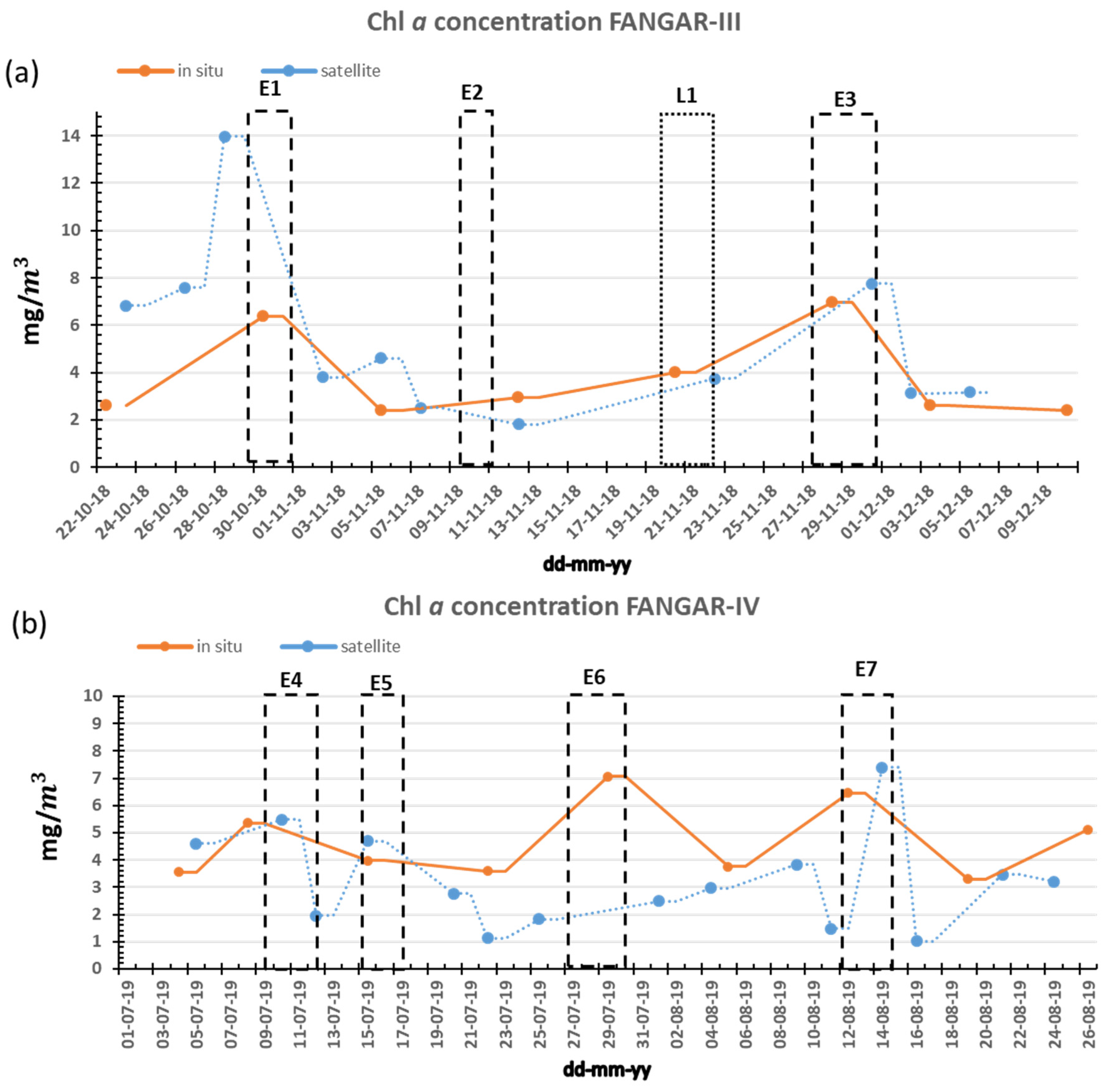
2.3. Chlorophyll Field Data Collection

Seawater samples were obtained using a silicone hose in order to obtain integrated water samples. For FANGAR-III, samples were collected at an inner point of the bay (C2, Figure 1) and at an outer point (O1, Figure 1) once a week. However, during FANGAR-IV, samples were collected monthly at six sampling stations (orange points (O1, M1, C1, C2, I, and SF) in Figure 1), both inside and outside the bay. The samples (1 L) were maintained in the dark inside a cool box until arrival to the laboratory 1–4 h after conducting the sampling. At arrival to the laboratory, the samples were immediately filtered through a Whatman glass fibre filter (GF/F) grade (47 mm diameter) under a low vacuum. The filters were maintained at −80 °C until analysis. For the analysis, the filters were immersed in 10 mL acetone 90%, ultrasound was applied for 5 min, and the tubes were maintained 24 h in the dark at 4 °C. After this time, the tubes containing the filters were centrifuged (4000 rpm) for 10 min at 4 °C, and the supernatant was analysed in a Turner Trilogy fluorimeter equipped with a 7200-046-W module for the Chlorophyll a Extracted—Non-Acidification method [29].

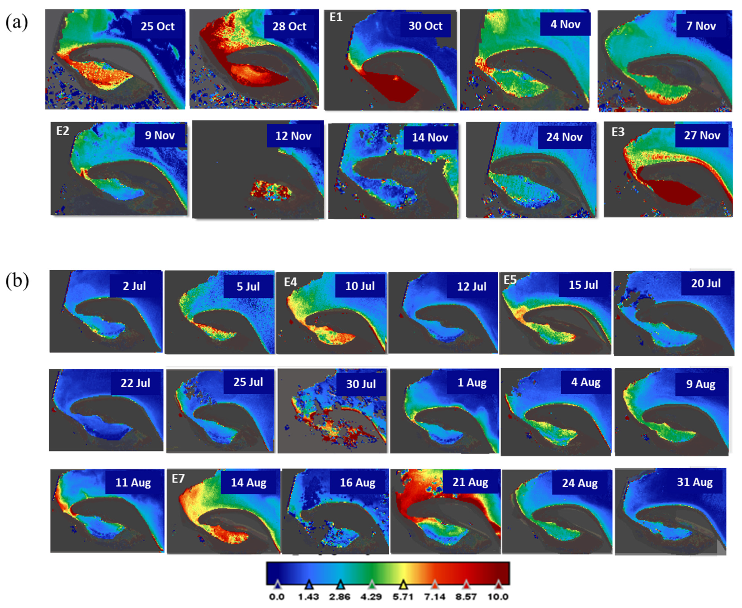
2.4. Chlorophyll Satellite Data Collection

The satellite images used were Sentinel-2A and Sentinel-2B, level 1-C, for the period of the campaigns. Sentinel-2A was launched on 23 June 2015, while Sentinel-2B was launched on 07 March 2017. Both are part of a European fleet of satellites aiming to deliver core data to the European Commission’s Copernicus program. L1C images (i.e., not cloud covered) were downloaded from Copernicus Open Access Hub (https://scihub.copernicus.eu/(accessed on 28 December 2020)). This level of processing includes radiometric and geometric corrections, including ortho-rectification and spatial registration on a global reference system with sub-pixel accuracy.

The Copernicus Sentinel-2 mission is comprised of a constellation of two polar-orbiting satellites placed in the same sun-synchronous orbit, phased at 180° to each other. The satellites carry a single optical instrument payload, the MultiSpectral Imager (MSI). The MSI samples 13 spectral bands in the visible-near infrared (VNIR) and short wave infrared (SWIR) spectral range at 3 different spatial resolutions (10, 20, and 60 m). It aims to monitor variability in land surface conditions, and its wide swath width (290 km) and high revisit time (10 days at the equator with one satellite, and 5 days with 2 satellites under cloud-free conditions, which result in 2–3 days at mid-latitudes) support monitoring of Earth’s surface changes. The coverage limits are from between latitudes 56° south and 84° north [30]. Chlorophyll a concentrations were computed automatically by the Sentinel Application Platform (SNAP) (https://step.esa.int/main/toolboxes/snap/ (accessed on 25 February 2021)) programme already tested in Soriano-González et al. [11]. The algorithm (NDCI, Normal Difference Chlorophyll Index developed by Mishra et al. [31]) and their corresponding neural networks are split into 2 parts: (i) retrieval of water-leaving reflectance (Rw) from Top of Atmosphere (TOA) reflectances (Rtoa), and (ii) retrieval of inherent optical properties (IOPs) from water-leaving reflectance Rw. The second part can also be used in conjunction with the standard atmospheric correction. All absorptions were normalized to the absorption at 443 nm; the absorption or scattering coefficients at this wavelength are the output of the IOP neural network. The MSI sensor has had an atmospheric correction applied to it with a C2RCC processor (Case 2 Regional CoastColour) [32] to obtain the Chl a images. The C2RCC processor is a multi-mission ocean colour processor, applicable to Sentinel-2 MSI, which relies on a large database of radiative transfer simulations inverted by neural networks [32]. These neural networks do not have a specification for the Ebro Delta. However, as seen in the work done by Soriano-González et al. [11], the algorithm used is a feasible, although not definitive, solution in this area.

3. Results

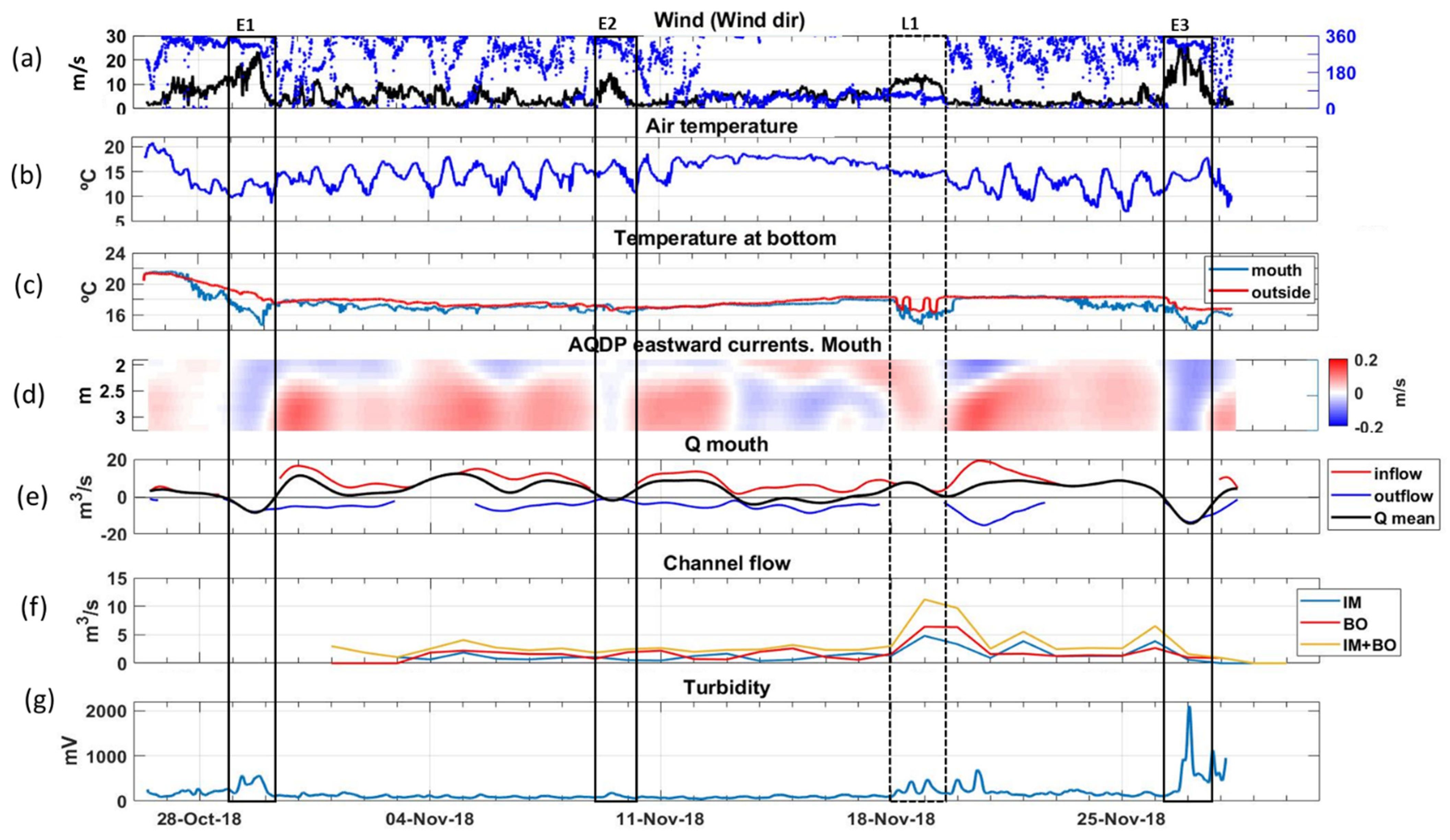
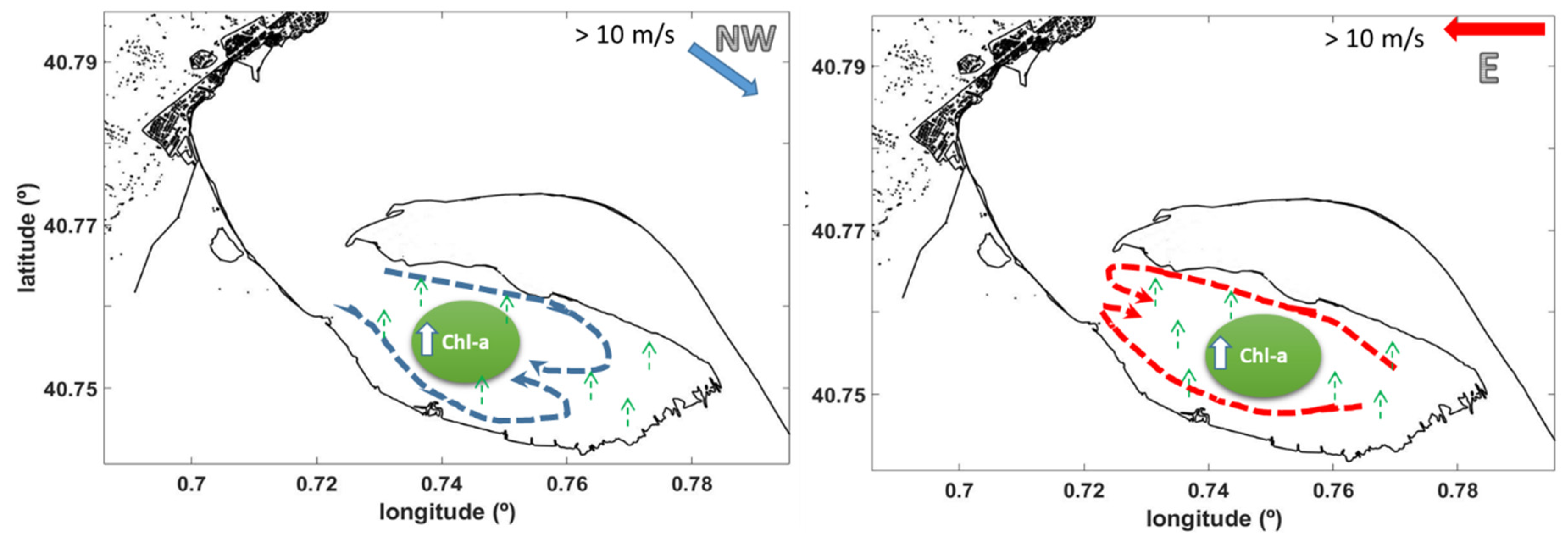
3.1. NW Wind Episode

The time series of the wind measured at the corresponding meteorological station are shown in Figure 2a and Figure 3a. During FANGAR-III, three episodes of NW winds were distinguished: 29–30 October, 9–10 November, and 27–29 November (identified as E1, E2, and E3, respectively). The intensity of the wind during these episodes was between 10–20 m·s⁻¹. During FANGAR-IV, four episodes of NW winds were distinguished: 9–10 July (E4), 15–16 July (E5), 27–29 July (E6), and 12–13 August (E7). During these episodes, the wind intensity was lower than during the previous campaign (no more than 10 m·s⁻¹). Only the E6 episode exceeded 10 m·s⁻¹.

NW cold winds cause cooling of the water in the bay [21], as well as a mixing of the water column. In Figure 2b and Figure 3b, it can see how the NW wind caused cooling in the air temperature, causing the water to cool down in turn (Figure 2c and Figure 3c). In addition, in Figure 2d and Figure 3d, it can be seen how the currents became outflow (blue colour) in the water column. This was corroborated with the flow, calculated from the integration of the currents of the water column, which became negative (Figure 2e and Figure 3e). This was also consistent with a vertical mixing of the water column due to the momentum transferred by the wind [9]. During both campaigns, turbidity data were collected with an OBS 3+. However, during the FANGAR-IV campaign the data recorded showed no feasible values and was not useful for the analysis. The data collected by the OBS during FANGAR-III, showed increases in turbidity during the NW episodes, marked in Figure 2g with black boxes. It means, during NW wind episodes (i.e., E1 to E7), the water circulation was characterised by outflow through the central channel and inflow in the lateral shoals. In addition, during episodes E1 to E3 an increase in turbidity was also observed (see Figure 2g). Chl a concentrations during strong NW wind episodes could also be observed using Sentinel-2 images (Figure 4). During the FANGAR-III period, fewer satellite images were available, and those that were available, some of them were of low quality due to the presence of clouds or to sun glitter that made satellite observation difficult. The images from the FANGAR-IV period were clearer and more meaningful. These images also showed increases in Chl a concentrations (approx. 5–8 mg·m⁻³) during these wind episodes, and a decay after these episodes.

Figure 5 shows the evolution of Chl a concentration during the field campaign. The episodes of NW winds are shown with boxes of dashed lines. In general, during all NW wind events, the concentration of Chl a concentration tended to increase, over 6 mg·m⁻³. For instance, values of Chl a concentration during E1 revealed larger values in comparison to precedent data. Discrepancies in the Chl a concentration during E2 were observed, likely associated with short episodes and less intensity in comparison to E1 or E3. This figure also shows that the satellite tended to overestimate (in the case of FANGAR-III) or underestimate (in the case of FANGAR-IV) the data in situ, but the temporal evolution of satellite data tended to follow the data collected during the filed campaign. However, the noted lack of high-frequency observations suggests a non-conclusive inter-comparison between both data sets. The picture during the summer field campaign also showed an increase in Chl a concentration during the NW episodes and a subsequent dropping of Chl a concentration when the wind calmed down. The increase in the E4 and E5 episodes was lower than in the other episodes (<6 mg·m⁻³), but the previous concentrations were around 3 mg·m⁻³, so the increase was clear. The E6 and E7 episodes showed peaks similar to the episodes of the previous campaign (over 6 mg·m⁻³). The vertical mixing response at strong wind events may be characterised by the Wedderburn number ($\mathrm{W}=(\mathsf{\Delta }{\rho \mathrm{gH}}^2{)/\mathrm{L}\mathsf{\tau }}_{\mathrm{W}}$ [9,33]), which evaluates the stabilization effect of the vertical stratification versus the destabilization effect of the wind. In the case of Fangar Bay, strong NW-NE winds (>10 m·s⁻¹) corresponding to W, was equal to 0.98 (i.e., W < 1), so the wind produced rapid, shear-driven mixing as the pycnocline tilted until it became almost vertical [9]. Note that there is a large difference between in situ and satellite data for the E6 event. This is also observed for the E1 episode. Some possibilities of these differences are explained in the discussion section. After all these Chl a concentration peaks, a sharp decrease in Chl a concentration could be observed (values of around 2 mg·m⁻³ in the FANGAR-III campaign, and 4 mg·m⁻³ in the FANGAR-IV campaign). Finally, comparing both campaigns, autumn Chl a concentrations showed larger mean values in comparison to the summer; however, the peak values during NW wind episodes showed similar values (for instance, 6.96 mg·m⁻³ during E3 and 7.06 mg·m⁻³ during E6).

3.2. E-NE Wind Episode

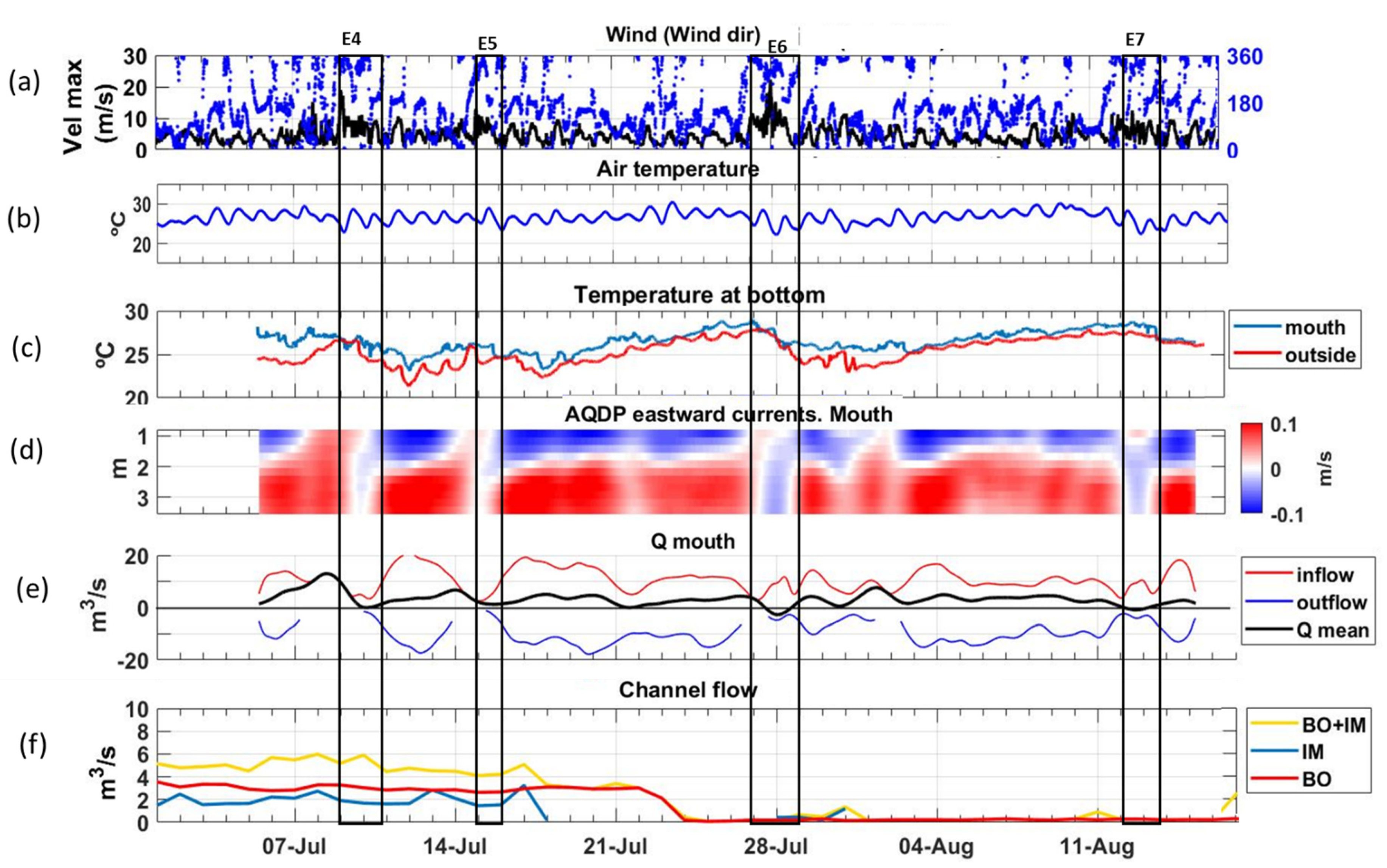
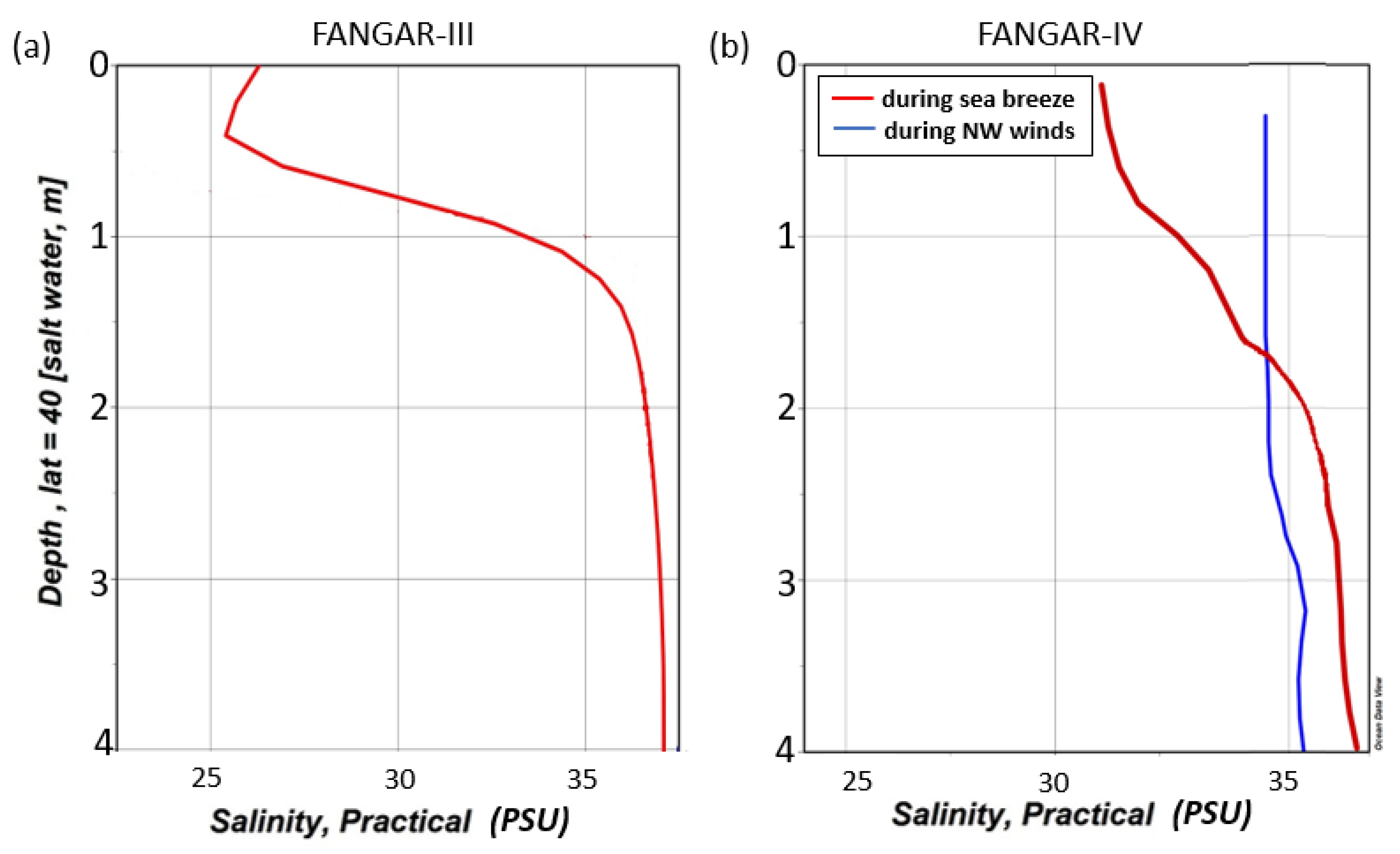
An easterlies wind episode, from 13 November to 20 November of 2018, was observed in Figure 2a (marked as dotted black box). An inversion of the positive estuarine circulation (i.e., outflow near the surface and inflow near the bottom) (Figure 2d) was observed during this wind episode. Specifically, from 18 to 20 November (L1), the wind intensity period (>10 m·s⁻¹) was associated with an inflow in the central channel of the mouth. This wind also caused a decrease in the water temperature, as can be seen in Figure 3c. Figure 5 shows in situ data measurement during this wind episode. A significant increase in Chl a concentration was observed (4 mg·m⁻³), and also for satellite data (3.9 mg·m⁻³) followed for a dropping of Chl a concentration in the subsequent days. The water circulation (Figure 2d) also showed a uniform pattern in the water depth (positive inflow), similar to NW winds episodes, suggesting vertical mixing occurred in the water column (no CTD surveys are available during this period). A small increase in bottom turbidity was also observed during this episode (Figure 2g). During the L1 episode, there were no satellite images, so we could not compare them with the data in situ.

3.3. Breeze Episode

During both campaigns, the sea breeze was characterised by daily southerlies with a wind intensity of 6 m·s⁻¹, as can be seen in Figure 2 (unmarked events). The water temperature during FANGAR-III ranged from 14 °C to 21.5 °C (Figure 3c), with an average of about 18 °C, both in the mouth and in the outer of the bay. During FANGAR-IV the water temperature range was between 21 °C and 29 °C (Figure 4c), with an average of 26 °C. According to CTD surveys, the wind was not able to mix the water column during the sea breeze, as can be seen from the average salinity profiles (Figure 6), so strong stratification prevailed due to freshwater inputs. In Figure 4 and Figure 5, in contrast to the NW wind episodes, during calm periods (breezes), low concentrations were observed (<4 mg·m⁻³). The Wedderburn number for the sea breeze episodes (winds about 6 m·s⁻¹) was equal to 2.75 (W >> 1) so that in this case, the pycnocline deepened slowly (see Figure 6) due to stirring [9].

3.4. Freshwater Inputs

During both campaigns, the irrigation channels were open (Figure 2f and Figure 3f), so the supply of nutrients was comparable. The flow rate was approximately 6 m³·s⁻¹ in both periods. During the FANGAR-III campaign, two peaks of freshwater input could be seen, from 19 to 22 November and during 26 November (Figure 2f). These peaks originated from an increased pumping of water. This coincided with the L1 episode, which caused more water to enter the bay. To prevent saltwater from entering the channels, rice farmers increase the volume of water pumped. During the FANGAR-IV campaign, freshwater inputs were observed during the first half of the campaign. After that, there is no data available for the IM point, and the contribution of BO was reduced to almost zero (Figure 3f).

The temporal variability of Chl a concentration with freshwater discharges did not show a significant correlation: R = 0.107 ($\rho$ < 0.05). The nutrient inputs that were discharged by the irrigation channels were presumably constant over time. This fact prevented us from checking if there was a correlation between freshwater discharges and Chl a concentration events since, during the field campaigns, the channels were always opened.

4. Discussion

Previous research in coastal bays and estuaries suggests that the typical temporal dynamics of Chl a concentration exhibit a seasonal cycle [10,16,34,35]. In the case of Ebro Delta Bays (i.e., Alfacs and Fangar), the seasonal cycle is dominated by the nutrient inflow from the irrigation channels, which reduce its water volume from January to March/April [16]. However, the impact on Chl a concentration during short term periods, such as wind episodes, remains unexplored, probably due to the lack of spatio-temporal data set resolution. Results from the FANGAR field campaigns (III and IV), jointly with remote sensing data, has brought a good opportunity to consider the Chl a concentration variability analysis over short time scales, and in particular, due to strong wind episodes and freshwater flow peaks.

The observations in Fangar Bay have shown an increase in the Chl a concentration after wind episodes. Proportionality of wind intensity and Chl a concentration increase seems consistent using in situ data. For instance, the increase in Chl a concentration during E1 was larger in comparison to E2 when the wind intensity was larger (E1 reached 15–20 m·s⁻¹ in comparison to E2, in which it was 10 m·s⁻¹). Nevertheless, a negligible correlation between wind and in situ Chl a concentration was observed: R = −0.16 ($\rho$ < 0.05) for FANGAR-III and R = −0.13 ($\rho$ < 0.05) for FANGAR-IV. During the FANGAR-III campaign, a time lag of 3 h between wind and Chl a concentration revealed a larger correlation than zero-lag correlation (R = 0.28 and R = 0.56 for satellite and in situ observations, respectively). However, the scarce or limited data set available suggest that further high-frequency measurements are needed to conclude lag correlations which would represent a delay between the wind episodes and the Chl a concentration growth response within the bay. Therefore, although qualitatively correspondence between strong wind episodes and Chl a concentration peaks (see Figure 5), future works should include intensive field campaigns to capture the effect of high-frequency behaviour on Chl a concentration evolution.

The intense wind episodes cause mixing in the water column according to the ADCP measurements (i.e., barotropic flow during wind episodes) and CTD surveys (homogeneous profiles in density). In this sense, two mechanisms responsible for an increase in Chl a concentrations during wind episodes may eventually occur: the resuspension of Chl a containing biomass and the supply of nutrients from the bottom to the water column [36,37,38]. Benthic algal (or microphytobentos) blooms may be resuspended by wind in coastal bays and estuaries [39]. The Chl a concentration is usually significantly higher in muddy substrates than in sandy substrates, as is the case in Fangar Bay [36]. Several authors [34,35,40] have discussed the presence of benthic microalgae that usually live in the first centimetres of the sediment according to water samples. Recently, Díez-Minguito and de Swart [37] demonstrated that as suspended sediment concentration increased, so did Chl a concentrations at spring and neap tidal scales due to simultaneous resuspension of sediment and Chl a containing biomass induced by tidal shear stress. In this sense, Grifoll et al. [41] showed evident relations in time-series observations in Alfacs Bay between strong wind events and an increase in near-bottom turbidity. Turbidity measurements in Fangar Bay (Figure 2g) have shown a relationship between the increase in near-bottom turbidity and intense wind episodes making plausible the incorporation of Chl a containing biomass in the water column during the wind episodes. Also, several remote sensing images shown in Figure 5 indicates that the highest concentrations of Chl a occur near the coastline (i.e., bay shoals) where light penetrates deeper in the water column, thereby favouring the growth of algal microorganisms at the bottom. The other mentioned mechanism of increasing Chl a concentration is related to the direct incorporation of nutrients from the bottom. In Ebro Delta coastal bays, several episodes of algal blooms have been reported and linked to increased nutrient concentrations [38,42], which were possibly triggered by resuspension mechanisms. The lack of correlation between the freshwater flow (associated with an increase in nutrients) and the short term increase in Chl a concentration within the bay may indicates a prevalence of the first hypothesis. Unfortunately, the lack of nutrients and full water column surveys during these wind episodes cannot confirm the importance of each one of the postulated hypothesis of Chl a concentration growing during energetic wind events. In this sense, Sarangi et al. [43] also showed that high concentrations of Chl a could be an indicator of surface water circulation driven particularly by local winds. Soriano-Gonzalez et al. [11] showed that when irrigation channels were closed in Fangar Bay, the wind could play a very important role, linking at a long-term scale, high Chl a concentrations increased with prolonged episodes of strong NW winds (i.e., winter and autumn). During sea-breeze conditions, when the wind intensity was lower in comparison to NW episodes, the Chl a concentration did not show a noticeable increase because the stratification remained unaltered (Figure 6). The low Chl a concentration periods during stratification in the water column also were found by Artigas et al. [16] in Alfacs Bay and Soriano-González et al. [11] for both bays (i.e., Fangar and Alfacs). The larger impact of NW and E-NE wind episodes (in comparison of sea-breeze) on Chl a concentration was due to the characteristics of the bay, which is very shallow and microtidal. In this sense, winds > 10 m·s⁻¹ (above typical sea-breezes intensities) immediately cause mixing in the water column and likely resuspension events [4,9,41]. Also, the duration of these strong winds associated with E-NE and NW events was a few days, compared to the strong winds that may occur during sea breeze periods, which are a few hours in length. In consequence, there are substantial arguments to associate the wind-induced resuspension (during NW and E-NE strong wind events) as a mechanism responsible for Chl a concentration increases, fueled by the supply of nutrients or biomass from the bottom of the water column.

The analysis in Fangar Bay of Chl a concentration evolution at short term scales and its response to energetic wind events may be useful in similar domains. In particular, to small bays, estuaries and lagoons in the Mediterranean Sea where the tide-induced hydrodynamics are limited and stratification of the water column tend to occur. However, coastal bays may show substantial differences due to the influence of their geometry and bathymetry in hydrodynamics, among other factors. For instance, Artigas et al. [16] observed substantial heterogeneity in the distribution of Chl a concentrations in Alfacs Bay, finding higher concentrations in the innermost area of the bay. Our observations have shown that the distribution of Chl a concentration in the Fangar Bay is more homogeneous throughout the bay during NW and E-NE wind episodes in comparison to Alfacs Bay. The small size of Fangar Bay (in comparison to Alfacs Bay; 56 km² vs. 12 km²) may contribute to these differences in spatial variability in Chl a concentration. The small-size suggest a short temporal scale to homogenize the water properties within the bay [9,44]. F-Pedrera et al. [9] used both ADCP data and numerical modelling to investigate the water circulation patterns in Fangar Bay. They found that the bathymetry effects may produce an axially symmetrical transverse structure with outflow on the axis of the central channel, opposite to the wind direction, alongside inflow in shallow lateral areas (see Figure 2d and Figure 3d). These water circulation patterns induce horizontal mixing within the bay due to the effectiveness of wind forcing in the shallowest areas of the bay. In this sense, the water circulation pattern within the bay may favour an increase in Chl a concentration during the wind episodes due to the redistribution of nutrients within the bay (not only from the resuspension events but also from the irrigation channels). Also, during intense NW wind episodes, satellite data showed a sharp transition of Chl a concentration near the mouth (see images from 30 October and 27 November in Figure 4) likely induced by a pushing effect of NW wind on surface waters near the mouth. These water circulation patterns also may favour an increase in Chl a concentration during and after intense NW wind episodes.

Inspired by the previous analysis of the wind episodes on Chl a concentration distribution, the increase in freshwater flow as a source of nutrients might be associated with an increase in Chl a concentration as has been suggested by several authors in a long-term analysis (see [10,11,16]). However, both in situ data and satellite images did not show an evident relation between Chl a concentration increase and freshwater peaks in the short-term. The variability shown by the freshwater inflow from the irrigation channels was low compared with the mean values (see Figure 2f and Figure 3f). Neither hydrodynamic variables (i.e., water currents) had a correlation with the freshwater peaks. The effect of irrigation is probably relevant at long-term scales (linked with the Chl a seasonal cycle reported) in comparison to the short-term variability of Chl a concentration, in which the effect seems negligible.

From a methodological perspective, satellite images have provided a valuable source of information on the spatial distribution of Chl a concentration in Fangar Bay. Sentinel-2 images showed that during the FANGAR-III campaign, Chl a concentrations were higher than during the FANGAR-IV campaign. Also, satellite data during the FANGAR-III campaign tended to overestimate in situ data, likely due to the satellite sensor capturing more suspended matter during autumn in comparison during summer. The Chl a concentration increasing was presumably linked to the increase in turbidity within the bay during the autumn due to the intense wind episodes (mainly NW wind episodes) increasing resuspension events [41]. Fangar Bay, as an example of a coastal and very shallow estuary, shows the limitations of the remote sensor to distinguish between Chl a concentration and suspended matter; in addition, the increased reflectance might also be related to bottom reflectance [11]. Another plausible effect on Chl a variability may be associated with the presence of mussels during summer in Fangar Bay that act as phytoplankton filter feeders. The mussel farming cycle begins at the end of the year, and the harvest ends in August-September [12], so in October–November, the presence of these filter feeders is scarce, allowing the phytoplankton to grow in greater numbers. In addition, high water advection rates typical of an estuary can lead to low productivity, even under conditions of high nutrient concentrations (i.e., open channels), if dilution rates are higher than phytoplankton growth rates [10]. In this case, the combined effect of resuspension events favoured by horizontal water transport within the bay during the autumn (in which NW episodes occur) may be co-responsible for larger concentrations of Chl a during the autumn in Fangar Bay.

The pattern of these two different situations of water circulation and their effects on Chl a concentrations in Fangar Bay are shown in Figure 7. According to the results, when the wind blew from the NW and from the E-NE, with an intensity of 10 m·s⁻¹ or more, there was a modification in the estuarine circulation, causing mixing throughout the water column and along the whole bay. This implies a homogenisation of the water column and an increase in Chl a concentration. When the sea breeze blows, the situation reinforces the stratification in the bay, causing a decrease in the concentration of Chl a.

The mussel and oyster farms in Fangar Bay has economic relevance in the Ebro Delta region. In this sense, it is important to know the distribution and dynamics of Chl a in Fangar Bay. This investigation may support decision-making strategies for local shellfish producers, regulating entities and stakeholders. Eventual relocation of mussels rafts or optimizing harvesting period activity may be benefited from an improved understanding of Chl a concentration evolution from episodic wind and freshwater discharge events for forecasting purposes [10,16,44].

5. Conclusions

Results based on intense field campaigns and Sentinel-2 images reveals that intense winds from both NW (offshore) and E-NE (onshore) cause an increase in the concentration of Chl a at the surface in Fangar Bay. Data have shown that there is a substantial correlation with wind peaks (e.g., NW wind episodes E3, E4, or E7) alternating negligible correlations periods. However, there are not enough Chl a data for outright affirmations. Even though the satellite data did not always coincide with the in situ data (sometimes overestimating and sometimes underestimating), both patterns were similar. The algorithm used for satellite image analysis (i.e., NDCI) still provides uncertain results for shallow coastal bays. It remains for future work to compare various existing methods for the processing of these type of images for Fangar Bay. The mechanisms responsible for the Chl a increase during wind episodes were the horizontal mixing and the bottom resuspension (also linked to the breakage of stratification) that presumably resuspends Chl a containing biomass and/or incorporates nutrients into the water column. On the other hand, sea-breeze is not capable of breaking up the stratification, so the Chl a concentration does not change significantly during sea-breeze events. It has been concluded that the mixing produced by strong winds favours an accumulation of Chl a concentration, while the stratification that causes a positive estuarine circulation reduces this accumulation. From our analysis freshwater peaks are a relevant factor for Chl a concentration evolution for long-term periods (i.e., intra-annual cycle); its variability was not correlated with the Chl a concentration evolution over the short-term. However, the biological and hydrodynamic linked processes are very complex and require additional field sampling focused on improving the spatio-temporal frequency of sampling during wind and freshwater peak episodes. In addition, the use of a coupled hydro-ecological numerical model could also help to understand these processes.

References

1. Geyer, W. Influence of Wind on Dynamics and Flushing of Shallow Estuaries. Estuar. Coast. Shelf Sci. 1997, 44, 713–722. [Google Scholar] [CrossRef]
2. Cloern, F.H.; Nichols, J.E. Time scales and mechanisms of estuarine variability, a synthesis from studies of San Fran-cisco Bay. Hydrobiologia 1985, 29, 229–237. [Google Scholar] [CrossRef]
3. Cerralbo, P.; Grifoll, M.; Valle-Levinson, A.; Espino, M. Tidal transformation and resonance in a short, microtidal Mediterranean estuary (Alfacs Bay in Ebre delta). Estuar. Coast. Shelf Sci. 2014, 145, 57–68. [Google Scholar] [CrossRef]
4. Cerralbo, P.; Grifoll, M.; Espino, M. Hydrodynamic response in a microtidal and shallow bay under energetic wind and seiche episodes. J. Mar. Syst. 2015, 149, 1–13. [Google Scholar] [CrossRef] [Green Version]
5. Cerralbo, P.; Espino, M.; Grifoll, M. Modeling circulation patterns induced by spatial cross-shore wind variability in a small-size coastal embayment. Ocean Model. 2016, 104, 84–98. [Google Scholar] [CrossRef]
6. Cerralbo, P.; Balsells, M.F.-P.; Mestres, M.; Fernandez, M.; Espino, M.; Grifoll, M.; Sanchez-Arcilla, A. Use of a hydrodynamic model for the management of water renovation in a coastal system. Ocean Sci. 2019, 15, 215–226. [Google Scholar] [CrossRef] [Green Version]
7. Sanay, R.; Valle-Levinson, A. Wind-Induced Circulation in Semienclosed Homogeneous, Rotating Basins. J. Phys. Oceanogr. 2005, 35, 2520–2531. [Google Scholar] [CrossRef] [Green Version]
8. Valle-Levinson, A.; Wong, K.-C.; Bosley, K.T. Observations of the wind-induced exchange at the entrance to Chesapeake Bay. J. Mar. Res. 2001, 59, 391–416. [Google Scholar] [CrossRef] [Green Version]
9. Balsells, M.F.-P.; Grifoll, M.; Espino, M.; Cerralbo, P.; Sánchez-Arcilla, A. Wind-Driven Hydrodynamics in the Shallow, Micro-Tidal Estuary at the Fangar Bay (Ebro Delta, NW Mediterranean Sea). Appl. Sci. 2020, 10, 6952. [Google Scholar] [CrossRef]
10. Llebot, C.; Sole, J.; Delgado, M.; Fernández-Tejedor, M.; Camp, J.; Estrada, M. Hydrographical forcing and phytoplankton variability in two semi-enclosed estuarine bays. J. Mar. Syst. 2011, 86, 69–86. [Google Scholar] [CrossRef]
11. Soriano-González, J.; Angelats, E.; Fernández-Tejedor, M.; Diogene, J.; Alcaraz, C. First Results of Phytoplankton Spatial Dynamics in Two NW-Mediterranean Bays from Chlorophyll-a Estimates Using Sentinel 2: Potential Implications for Aquaculture. Remote Sens. 2019, 11, 1756. [Google Scholar] [CrossRef] [Green Version]
12. Ramón, M.; Fernández, M.; Galimany, E. Development of mussel (Mytilus galloprovincialis) seed from two different origins in a semi-enclosed Mediterranean Bay (N.E. Spain). Aquaculture 2007, 264, 148–159. [Google Scholar] [CrossRef]
13. D’Ortenzio, F.; D’Alcalà, M.R. On the trophic regimes of the Mediterranean Sea: A satellite analysis. Biogeosciences 2009, 6, 139–148. [Google Scholar] [CrossRef] [Green Version]
14. Morales-Blake, A.R. Estudio Multitemporal de la Clorofila Superficial en el mar Mediterráneo Noroccidental, Evaluada a Partir de datos SeaWIFS: Septiembre de 1997 a Agosto del 2004. Ph.D. Thesis, University of Barcelona, Barcelona, Spain, 2006. [Google Scholar]
15. Jou, S.; Folch, A.; Garcia-Orellana, J.; Carreño, F. Using freely available satellite thermal infrared data from Landsat 8 to identify groundwater discharge in coastal areas. Geophys. Res. Abstr. 2019, 21, 1. [Google Scholar]
16. Artigas, M.; Llebot, C.; Ross, O.; Neszi, N.; Rodellas, V.; Garcia-Orellana, J.; Masque, P.; Piera, J.; Estrada, M.; Berdalet, E. Understanding the spatio-temporal variability of phytoplankton biomass distribution in a microtidal Mediterranean estuary. Deep. Sea Res. Part II Top. Stud. Oceanogr. 2014, 101, 180–192. [Google Scholar] [CrossRef]
17. Demers, S.; LaFleur, P.E.; Legendre, L.; Trump, C.L. Short-Term Covariability of Chlorophyll and Temperature in the St. Lawrence Estuary. J. Fish. Res. Board Can. 1979, 36, 568–573. [Google Scholar] [CrossRef]
18. Geyer, N.L.; Huettel, M.; Wetz, M.S. Phytoplankton Spatial Variability in the River-Dominated Estuary, Apalachicola Bay, Florida. Chesap. Sci. 2018, 41, 2024–2038. [Google Scholar] [CrossRef]
19. Masson, D.; Peña, A. Chlorophyll distribution in a temperate estuary: The Strait of Georgia and Juan de Fuca Strait. Estuar. Coast. Shelf Sci. 2009, 82, 19–28. [Google Scholar] [CrossRef]
20. Delgado, M.; Camp, J. Abundancia y distribución de nutrientes inorgánicos disueltos en las bahías del delta del Ero. Inv. Pesq. 1987, 51, 427–441. [Google Scholar]
21. Garcia, M.A.; Ballester, A. Notas acerca de la meteorología y la circulación local en la región del delta del Ebro. Inv. Pesq. 1984, 48, 469–493. [Google Scholar]
22. Archetti, G.; Bernia, S.; Salvà-Catarineu, M. Análisis de los vectores ambientales que afectan la calidad del medio en la bahía del Fangar (Delta del Ebro) mediante herramientas SIG. Rev. Int. Cienc. Tecnol. Inf. Geogr. 2010, 10, 252–279. [Google Scholar]
23. Bolaños, R.; Jorda, G.; Cateura, J.; Lopez, J.; Puigdefàbregas, J.; Gómez, J.; Espino, M. The XIOM: 20 years of a regional coastal observatory in the Spanish Catalan coast. J. Mar. Syst. 2009, 77, 237–260. [Google Scholar] [CrossRef] [Green Version]
24. Grifoll, M.; Navarro, J.; Pallares, E.; Ràfols, L.; Espino, M.; Palomares, A. Ocean–atmosphere–wave characterisation of a wind jet (Ebro shelf, NW Mediterranean Sea). Nonlinear Process. Geophys. 2016, 23, 143–158. [Google Scholar] [CrossRef] [Green Version]
25. Muñoz, I. Limnología de la part baixa del riu ebre i els canals de reg: Els factors fisico-quimics, el fitoplancton i els macroinvetebrats bentonics. Tesis para la postulación al grado de doctor. Ph.D. Thesis, Departamento de Ecología, Facultad de Biología, Universidad de Barcelona, Barcelona, Spain, 1990. [Google Scholar]
26. Automatic Water Quality Information System, DEL EBRO, CHE-Hydrographic Confederation, Quality Alert Network, SAICA Project. 2013. Available online: https://www.saica.co.za/ (accessed on 30 January 2020).
27. Perez, J.; Marta, C. Distribución espacial y biomasa de las fanerógamas marinas de las bahías del delta del Ebro. Inv. Pesq. 1986, 50, 519–530. [Google Scholar]
28. Camp, J.; Delgado, M. Hidrogafia de las bahías del delta del Ebro. Inv. Pesq. 1987, 51, 351–369. [Google Scholar]
29. Welschmeyer, N.A. Fluorometric analysis of chlorophyll a in the presence of chlorophyll b and pheopigments. Limnol. Oceanogr. 1994, 39, 1985–1992. [Google Scholar] [CrossRef]
30. ESA. SENTINEL-2 User Handbook; ESA: Pairs, France, 2015. [Google Scholar]
31. Mishra, D.R.; Mishra, S. Normalized Difference Chlorophyll Index: A Novel Model for Remote Estimation of Chloro-phyll-a Concentration in Turbid Productive Waters. Remote Sens. Environ. 2012, 117, 394–406. [Google Scholar] [CrossRef]
32. Brockmann, C.; Doerffer, R.; Peters, M.; Stelzer, K.; Embacher, S.; Ruescas, A. Evolution of the c2rcc neural network for sentinel 2 and 3 for the retrieval of ocean colour products in normal and extreme optically complex waters. Living Planet Symp. 2016, 740, 54. [Google Scholar]
33. Shintani, T.; De La Fuente, A.; Niño, Y.; Imberger, J. Generalizations of the Wedderburn number: Parameterizing upwelling in stratified lakes. Limnol. Oceanogr. 2010, 55, 1377–1389. [Google Scholar] [CrossRef]
34. De Madariaga, I. Photosynthetic Characteristics of Phytoplankton during the Development of a Summer Bloom in the Urdaibai Estuary, Bay of Biscay. Estuar. Coast. Shelf Sci. 1995, 40, 559–575. [Google Scholar] [CrossRef]
35. Pinckney, J.L.; Paerl, H.W.; Harrington, M.B.; Howe, K.E. Annual cycles of phytoplankton community-structure and bloom dynamics in the Neuse River Estuary, North Carolina. Mar. Biol. 1998, 131, 371–381. [Google Scholar] [CrossRef]
36. Delgado, M. Abundance and distribution of microphytobenthos in the bays of Ebro Delta (Spain). Estuar. Coast. Shelf Sci. 1989, 29, 183–194. [Google Scholar] [CrossRef]
37. Díez-Minguito, M.; De Swart, H.E. Relationships between Chlorophyll-a and Suspended Sediment Concentration in a High-Nutrient Load Estuary: An Observational and Idealized Modeling Approach. J. Geophys. Res. Oceans 2020, 125. [Google Scholar] [CrossRef]
38. Loureiro, S.; Garcés, E.; Fernández-Tejedor, M.; Vaqué, D.; Camp, J. Pseudo-nitzschia spp. (Bacillariophyceae) and dissolved organic matter (DOM) dynamics in the Ebro Delta (Alfacs Bay, NW Mediterranean Sea). Estuar. Coast. Shelf Sci. 2009, 83, 539–549. [Google Scholar] [CrossRef] [Green Version]
39. De Jorge, V.N.; Van Beusekom, J.E.E. Wind- and tide-induced resuspension of sediment and microphytobenthos from tidal flats in the Ems estuary. Limnol. Oceanogr. 1995, 40, 776–778. [Google Scholar] [CrossRef] [Green Version]
40. Sondergaard, M.; Kristensen, P.; Jeppesen, E. Phosphorus release from ressuspended sediment in the shallow and wind-exposed Lake Arreso, Denmark. Hydrobiologia 1992, 228, 91–99. [Google Scholar] [CrossRef]
41. Grifoll, M.; Cerralbo, P.; Guillén, J.; Espino, M.; Hansen, L.B.; Sánchez-Arcilla, A. Characterization of bottom sediment resuspension events observed in a micro-tidal bay. Ocean Sci. 2019, 15, 307–319. [Google Scholar] [CrossRef] [Green Version]
42. Roque, A.; Lopez-Joven, C.; Lacuesta, B.; Elandaloussi, L.; Wagley, S.; Furones, M.D.; Ruiz-Zarzuela, I.; De Blas, I.; Rangdale, R.; Gomez-Gil, B. Detection and identification of tdh- And trh-positive Vibrio parahaemolyticus strains from four species of cultured bivalve molluscs on the Spanish Mediterranean coast. Appl. Environ. Microbiol. 2009, 75, 7574–7577. [Google Scholar] [CrossRef] [PubMed] [Green Version]
43. Sarangi, R.K.; Nayak, S.; Panigraphy, R.C. Monthly variability of chlorophyll and associated physical parameters in the southwest Bay of Bengal water using remote sensing data. Indian J. Mar. Sci. 2008, 37, 256–266. [Google Scholar]
44. Llebot, C.; Rueda, F.J.; Sole, J.; Artigas, M.L.; Estrada, M. Hydrodynamic states in a wind-driven microtidal estuary (Alfacs Bay). J. Sea Res. 2014, 85, 263–276. [Google Scholar] [CrossRef]
Figure 1. Location of the study area. The red circles show the two main points of freshwater discharges (Bassa de les Olles (BO) and Illa de Mar (IM)), the red diamonds show the two mooring locations during the field campaigns (M: Mouth; O: Out of the bay), and the green triangle shows the location of the meteorological station (Met and Met_Amp). The black point shows the Conductivity, Temperature, and Depth (CTD) profile, the black points surrounded by an orange circle as well as the orange letters (M: Mouth; C: Central; SF: Selfish Farms; I: Interior) are the chlorophyll a (Chl a) water sampling stations and the blue lines show the bathymetry.
Water 13 00701 g001
Figure 2. From top to bottom, wind intensity and direction (a), air temperature (b), bottom water temperature (c) alongshore currents in mouth (d), inflow (positive) and outflow (negative) of bay (e), flow of the discharge channels (f), turbidity (g). The black boxes show the events of the NW, and the dotted black boxes show the events of the E, from 26 October to 28 November 2018 (FANGAR-III). E1: 29–30 October; E2: 9–10 November; L1: 18–20 November; E3: 27–29 November.
Water 13 00701 g002
Figure 3. From top to bottom, wind speed (a), air temperature (b), bottom water temperature (c) alongshore currents in mouth (d), inflow and outflow of the mouth (e), flow of the discharge channels (f). The black boxes show the events of the NW from 5 July to 6 September 2019 (FANGAR-IV). E4: 9–10 July; E5: 15–16 July; E6: 27–29 July; E7: 12–13 August.
Water 13 00701 g003
Figure 4. Sentinel-2 images during FANGAR-III (a) and during FANGAR-IV (b). The wind episodes are marked in each corresponding image with white letters. Episodes L1 and E6 did not match with any satellite image, so they are not represented in the figure.
Water 13 00701 g004
Figure 5. Time series of Chl a concentration in situ and satellite images, at a central point in the bay for FANGAR-III (a) and FANGAR-IV (b). The boxes with dashed line mark the episodes of the NW wind, while the dotted box marks the episodes of the E-NE wind.
Water 13 00701 g005
Figure 6. Average salinity profiles from FANGAR-III (a) and from FANGAR-IV (b) from CTD surveys.
Water 13 00701 g006
Figure 7. Water circulation and Chl a concentration patterns in Fangar Bay. The dashed lines show the water circulation within the bay, and the blue and red arrow shows the wind direction, including the wind intensity minimum value (approx.) for stratification breakage and consequently an increase in the Chl a concentration. The small green arrows show the resuspension of matter (nutrients or Chl a-containing biomass) from the bottom caused by winds.
Water 13 00701 g007