
Effective Drought Communication: Using the Past to Assess the Present and Anticipate the Future


1
KERMIT, Department of Data Analysis and Mathematical Modelling, Ghent University, Coupure Links 653, 9000 Ghent, Belgium
2
Hydro-Climate Extremes Lab., Ghent University, Coupure Links 653, 9000 Ghent, Belgium
*
Author to whom correspondence should be addressed.
Water 2021, 13(5), 714; https://doi.org/10.3390/w13050714
Submission received: 21 January 2021
/
Revised: 1 March 2021
/
Accepted: 2 March 2021
/
Published: 5 March 2021
(This article belongs to the Section Water Resources Management, Policy and Governance)
Abstract
:Especially during drought events, it is important that water gets properly allocated and is not misused or wasted. For an effective drought management, it is thus of utmost importance to raise the awareness of water managers as well as the general public about the drought’s severity. In this paper, we provide two possible sources of information that can be used to communicate about drought events. To illustrate our approach, we make use of drought events that were identified in preceding work as connected components in space and time through the use of operators from the field of mathematical morphology and summarized in terms of characteristics such as affected area, duration and intensity. We demonstrate how these drought characteristics can be used to query for historical drought events that are most similar to an ongoing event, such that lessons learnt from the management of past events can be incorporated in the management of the ongoing event. Further, we also demonstrate how a probabilistic model describing the dependence structure between the drought characteristics is identified and how such model can serve as a basis to estimate the severity of the event. Both approaches provide information that can be used to communicate to laymen about the severity of the ongoing drought, which will help them to anticipate the future.
1. Introduction
Crop failure, water scarcity and reduced energy supply are examples of severe socio-economic consequences drought events can incur. Major drought events can even lead to serious human conflicts. Commonly, four types of drought events are distinguished [1]. A deficiency in precipitation over a large area and a prolonged period of time is the primary cause of a drought event [2] and is regarded as a meteorological drought. The combination with high evaporation rates can result in a large period of low soil moisture and, hence, lead to an agricultural drought as crops become affected. In a later stage, the recharge to aquifers and rivers may be reduced and a hydrological drought develops. When water demands cannot be met by the water supply systems and economic activities and ecosystems seriously suffer, a socio-economic drought is experienced [1,2,3].
On-site, one can relatively easily tell when one is experiencing a drought event. Yet, operationally identifying a drought event on the basis of data is not that easy. Droughts have no clear start and end, they can last for several months or years and progress from one place to another. Furthermore, their intensity changes with place and time. As such, a drought event may be more severe than what is being experienced at a certain location. Yet, in the management of a drought, it is important to account for the full extent of the drought as measures in one area may affect the water availability in another one.
When coping with drought events, it is very important to motivate people not to waste water. Only if people are fully aware of the severity of the current situation, such a message will be echoed and people will be encouraged to follow the measures taken to mitigate (near-)future dramas. Communication plays a crucial role in creating public awareness. To that end, several options exist. However, most of the existing drought indices will not be useful for this purpose as they are generally not understood by laymen and even not by water managers in the field. In this paper, we address two options that make it possible for the general public to assess the severity of the drought situation. The first option is to compare the current drought situation to that of a historical drought. The second option addresses the following question: what is the chance that an even worse drought would occur? In this paper, the methodology is presented for providing an answer for both options. To illustrate the approach, we make use of a database containing characteristics of drought events in mainland Australia as characterised by Vernieuwe et al. [4].
In the first application, we illustrate how the characteristics of an ongoing drought event, as experienced so far, can be compared with those of historical drought events. By retrieving the most similar historical drought events, lessons learnt from past actions or non-actions can be put into practice in order to improve the measures taken to cope with the ongoing event. In the second application, a probabilistic copula-based model is identified on the basis of which the probability of obtaining a more severe or supercritical event, i.e., an event more severe than the ongoing event, can be computed. This value can then be used in a communication strategy to increase public awareness of the rareness of the ongoing event such that mitigation measures, such as a reduced water use, get respected.
The methodology presented here differs from the Severity-Area-Duration (SAD) approach [5], as for constructing SAD curves also partial drought events are selected and no copulas are involved in describing the dependence between the variables. It also differs from the approach using drought severity–duration–frequency curves [6], as in the latter approach the extent of the drought events is not accounted for.
Copulas are commonly used to model the dependence between two random variables in a flexible way as, in contrast to the modelling by e.g., a bivariate Gaussian distribution, this modelling is performed independently of the univariate marginal distributions of the random variables. Ample applications in hydrology have already used copulas (see, among others, Pham et al. [7], Salvadori and De Michele [8], Serinaldi et al. [9], Song and Singh [10], Vandenberghe [11], Wong et al. [12]). However, whenever the dependence between more than two random variables needs to be modelled, the use of multivariate copulas is not that popular as the theory becomes more complicated than in the bivariate case [11]. Yet, vine copulas [13,14,15] have been introduced such that the multivariate dependence can be modelled on the basis of a mixing of (conditional) bivariate copulas. Because of their flexibility, also vine copulas are gaining popularity and are used in many hydrological applications (see, among others, Pham et al. [7], Erhardt and Czado [16], Hao and Singh [17], Pham et al. [18], Shafaei et al. [19]).
As stated before, this paper introduces two options that allow for a more effective communication about droughts. To demonstrate this, we make use of a database assembled by Vernieuwe et al. [4]. Yet, other databases could have been used as well. To provide some insight in this database, Section 2 briefly explains both the data used and the methodology that was used for the delineation of the drought events. Section 3 exemplifies how drought events that are most similar to an ongoing event can be queried on the basis of the characteristics of the ongoing and historical drought events. Section 4 elaborates on how one can derive the probability of obtaining a more severe drought event. For this purpose, copulas and vine copulas are briefly introduced and the use of a vine copula model for determining the probability that a more severe drought event can be experienced, is illustrated. This section also shows how a copula can be employed to distinguish subcritical from supercritical events. Section 5 then formulates the conclusions.
2. Data Set and Data Pre-Processing
The data set used in this paper is obtained from Vernieuwe et al. [4] and contains drought events in mainland Australia that were derived from the GLEAM v3.0a data set [20,21] for the period from 1 January 1980 till 31 December 2014. The GLEAM data set consists of daily root-zone soil moisture values at a 0.25° resolution. As explained in Martens et al. [20], the data have been estimated on the basis of satellite-observed soil moisture, vegetation optical depth and snow water equivalents, reanalysis air temperature and radiation and a multi-source precipitation product. This data set shows a slighter higher quality compared to other GLEAM data sets when evaluated against in situ measured soil moisture data [20]. As Australia is regarded as being vulnerable to the expected drying trend of the next 50–100 years [22], daily data covering mainland Australia were selected from this data set. The daily soil moisture values of the data set were first reprojected to the Lambert Azimuthal Equal Area coordinate system with a resolution of 27.442 km × 29.079 km.
Following the idea of Sheffield et al. [23] and Sheffield and Wood [24], percentile values of soil moisture were used as this allows for a fair comparison between values at different locations. On the basis of a neighbourhood identified around the pixel of interest, the empirical cumulative distribution function for this neighbourhood was established and the soil moisture value corresponding to the 10th percentile was identified. Values below this soil moisture threshold then indicate that drought conditions are met. By doing so, a time series of thresholded soil moisture images was obtained. From this time series, Vernieuwe et al. [4] then identified the drought events as connected components in space and time through the application of operators borrowed from mathematical morphology [25]. The purpose of these morphological operators is to simplify images by retaining the essential information and removing irrelevancies [26]. These morphological operators make use of the basic operators erosion and dilation in order to remove salt-and-pepper noise.
To these delineated drought events, intensity, affected area and duration were assigned as drought characteristics. The intensity and the affected area were derived as a weighted average of the five largest daily values of the drought event, with decreasing weights for decreasing values. This ensures that a drought is not fully characterised by an extent or a maximal intensity only observed at one particular day, but that these characteristics are representative of a longer period. We refer to Vernieuwe et al. [4] for a detailed explanation of the delineation of drought events, in particular of how the weights used for averaging were set.
In this paper, the database assembled by Vernieuwe et al. [4] containing the different drought events with their corresponding intensity, affected area and duration, was used as a basis for developing the two applications that are described in the following sections. Of course, one could opt for an alternative approach to delineate the drought events, or calculate the drought characteristics in a different manner.
3. Querying for the Most Similar Drought Event
When one is experiencing a drought event, it might be helpful for a water manager to relate the ongoing drought event to historical drought events in order to better cope with the event. Of course, one cannot predict the duration and intensity of and the area covered by the drought event. Yet, as the drought event is proceeding, one might learn lessons from past actions taken during a historical drought event that is similar to the one that is being faced so far. This may then help to better estimate whether or not ongoing measures may be adequate.
On the basis of drought characteristics, one is able to compute a degree of similarity between the ongoing and the past drought events. To do so, the obtained values of the characteristics are first transformed to such that the order of magnitude of the different characteristics (e.g., the intensity takes values in the unit interval , while the affected area reaches values larger than 105 km2) does not influence the measure used. This transformation can be accomplished by using the empirical cumulative distribution functions of the characteristics. Further, the similarity between the past drought events and the ongoing drought event can then be expressed by using the (Manhattan) distance (the sum of absolute differences), i.e., the drought event whose characteristics are situated closest to those of the ongoing drought event is then regarded as the most similar drought event. However, as it might be more helpful to water managers to focus on drought events that were at least as severe as the ongoing drought event, the search space in which the most similar historical drought event is queried for, is restricted towards drought events for which the values in are slightly smaller than or effectively larger than these of the ongoing drought event:
with the point in corresponding to the drought characteristics of the ongoing drought event, Z the set of points corresponding to the drought characteristics of the historical drought events, and the point in corresponding to the most similar historical drought event. By specifying , the search space is restricted to drought events for which the values of the characteristics in are slightly smaller or effectively larger than those of the ongoing event.
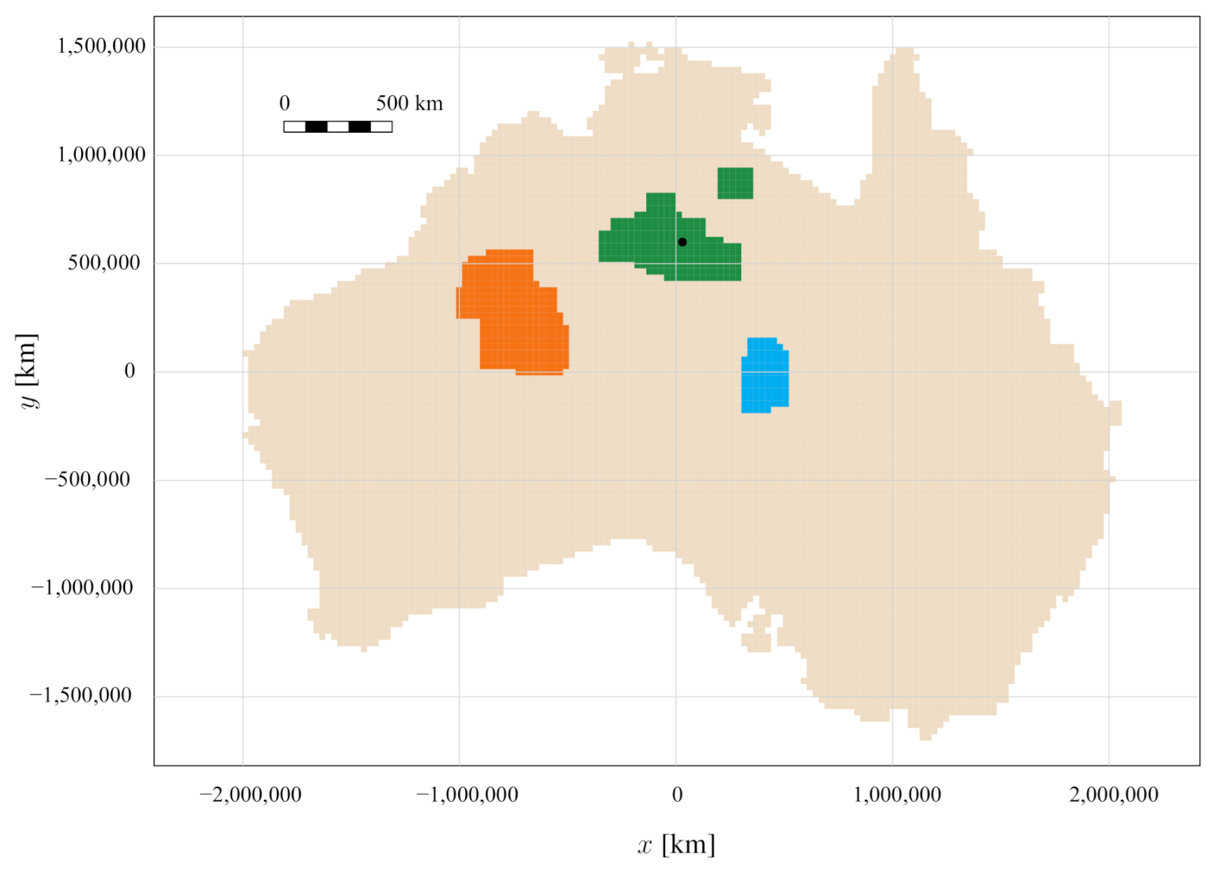
For instance, assume that the present is 2 November 2012, and that an ongoing drought event is experienced at the location indicated by the black dot in Figure 1. For water managers, it can then be interesting to know which of the historical drought events in the database best resembles the ongoing drought event. To do so using the above-described method, the characteristics of the ongoing event since its beginning until 2 November 2012 are determined as this day is regarded as the present. Table 1 lists the characteristics of the ongoing drought event and in the first line the characteristics of its most similar drought event according to Equation (1). One can see that the most similar drought event has a slightly smaller affected area, a 29 days longer duration and is less intense than the ongoing drought event. Yet, water managers might consider it to be more informative to learn from measures taken for more than one similar historical drought event as drought characteristics might be different. Therefore, the k most similar drought events, i.e., the top- k similar drought events, can be selected according to Equation (1). The number of similar drought events to retrieve can easily be decided by the water managers themselves. Table 1 lists as an example the characteristics of the top-3 similar drought events. One can already see that the affected area and the duration can substantially differ between the selected events. Ìt is important to remark that it is essential to repeat this exercise while a drought is evolving, as its characteristics will change over time. Therefore, other historical droughts may become more comparable than the ones that have been identified before.
Alternative interesting queries can also be performed in order to inform people on-site about most similar historical drought events for the given location or time of the year. In the first case, a constrained query has to be performed such that only drought events that affected the given location can be returned by the query. For instance, for the location indicated by the black dot in Figure 1, other historical drought events also might have affected this location. By constraining the query to only these drought events, most similar drought events might be obtained for which the people on-site might show more affinity. In the second case, the query can be constrained to the given time of year. For instance, one might wonder which most similar historical drought event also contained November the 2nd.
Table 1 shows the results of the constrained query for droughts at the location of the black dot in Figure 1 that are similar to the ongoing drought event. One can already see that two of the three most similar drought events listed in this table were drought events that occurred at the location indicated in Figure 1. The third drought event listed in Table 1 was a drought event that affected the South-East of Australia. The characteristics of the third drought event do not majorly differ from those of the similar drought events given in Table 1. It was noted when performing this constrained query that only four drought events met the severity (see Equation (1)) and the location constraint. Only from these four drought events the (three) most similar drought events had to be selected. When one is interested in finding similar drought events that occurred in a specific region, province, etc., this location-specific query can of course be extended. Regarding the most similar drought events that also contained November the 2nd (in some year between 1980 and 2014), the same events as for the location-specific query were found. Also in this case, only six drought events met the constraints. Similarly as for the location-specific query, this time-specific query can be extended to retrieve drought events that took place during some specified period of the year.
4. Probabilistic Comparison of the Ongoing Drought Event to Historical Drought Events
On the basis of a probabilistic model, fitted to the identified drought characteristics, questions may be answered about the probability that historical drought events were less severe than the one being experienced. To do so, a flexible probabilistic model that incorporates the existing dependence structure between two or more stochastic variables, independently of their marginal distributions, i.e., a copula, is used. A bivariate copula or 2-copula is a function that satisfies:
- for all , ∈ ,
- for all , , , ∈ for which ≤ and ≤ :
For two random variables and , a bivariate copula combines their marginal cumulative distributions and into the bivariate cumulative distribution function :
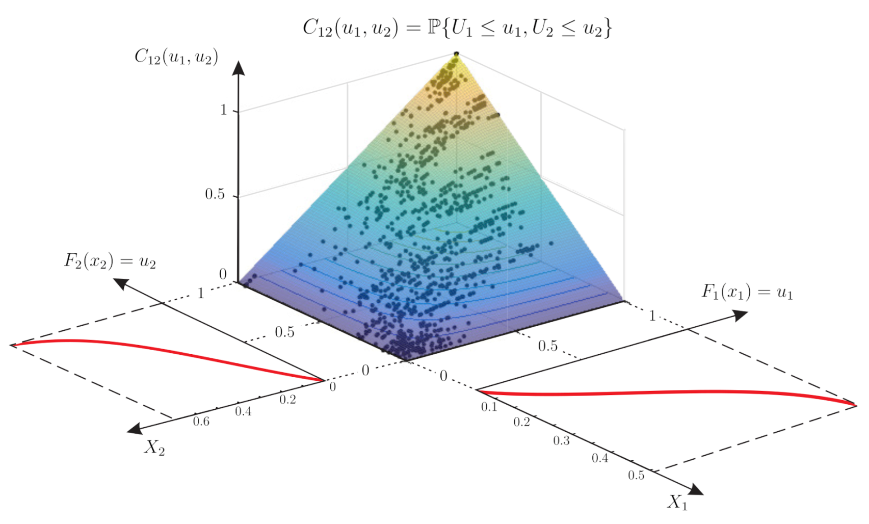
which is also known as the theorem of Sklar [27]. Here, , , and are values of the random variables , , and , with and uniformly distributed on . This theorem is crucially important as it allows for the modelling of the joint distribution function to be performed in two independent steps [8,28]: firstly, the modelling of the marginal distribution functions and, secondly, the modelling of the dependence structure. Figure 2 explains the concept of a copula and how the marginal distribution functions are related to the copula. This figure shows the transformation of two random variables and to the uniform random variables and by means of their cumulative distribution functions and . Given a data set with data points , , with n the number of data points, a copula is fitted to the couples of transformed values of and describes the dependence between the variables and and hence between and .
The theory of bivariate copulas can be extended to multivariate copulas such that the dependence between more than two variables can be modelled. Yet, using multivariate copulas has several drawbacks such as the increase in dimensionality which complicates the theory of multivariate copulas [11]. In order to mitigate the disadvantages of using multivariate copulas, a vine copula, a flexible construction method based on the mixing of two-dimensional copulas, has been introduced in the work of Bedford and Cooke [15]. Vine copulas have already shown their potential in financial (see, among others, Pircalabu and Jung [29], Zhang [30], Al Janabi et al. [31]) and hydrological applications (see, among others, Pham et al. [7], Erhardt and Czado [16], Hao and Singh [17], Pham et al. [18], Shafaei et al. [19]).
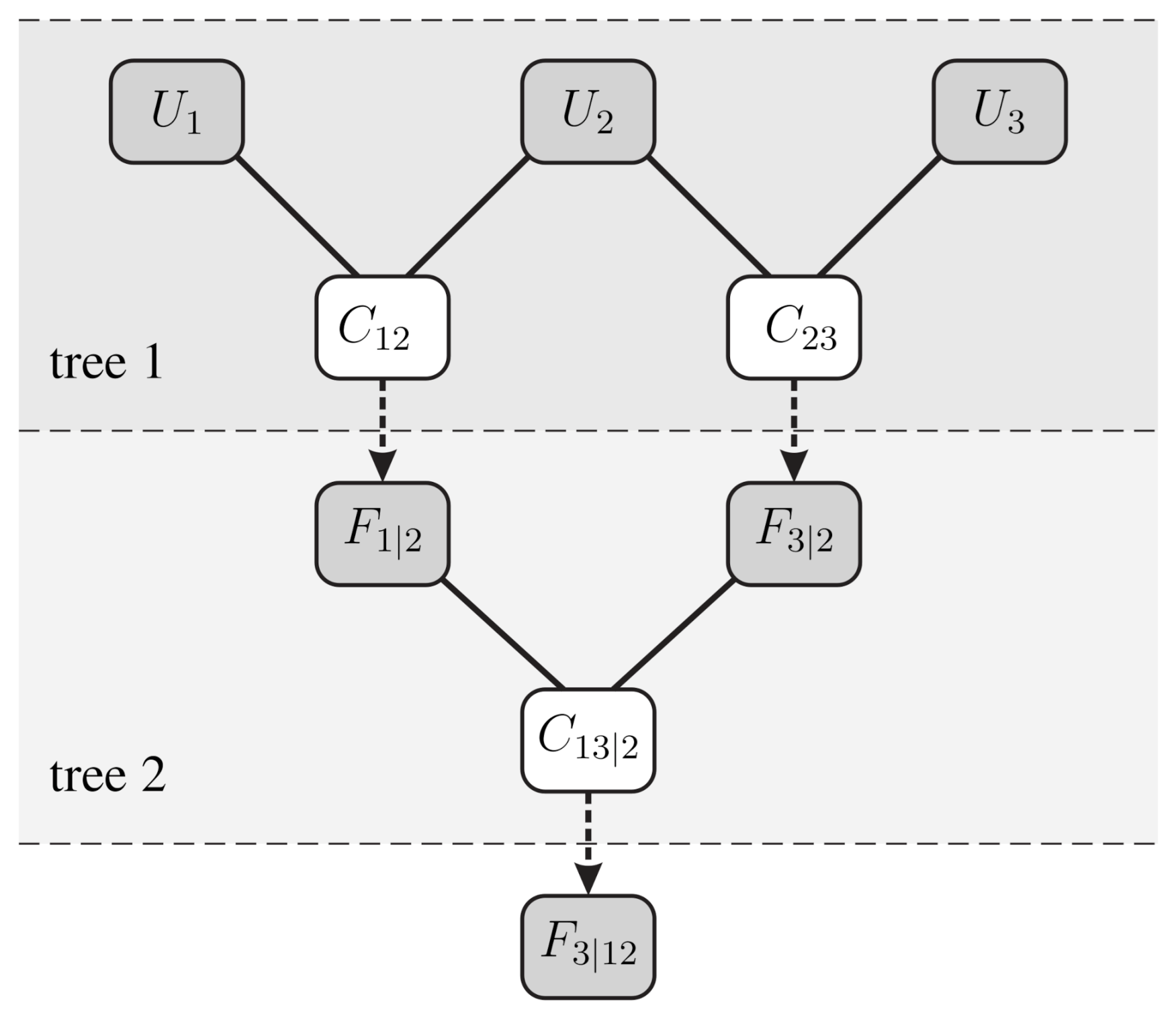
Figure 3 schematically represents the structure of a three-dimensional vine copula. In the first tree, two copulas are fitted to the values of the variables and and to the values of and . Recall that these variables are the transformed variables of the random variables , and . On the basis of these two copulas and , the conditional distributions and can be determined as follows:
Using these expressions, for all values of , the values in the conditional cumulative distribution functions can be calculated. These values then serve as input to fit another copula , as illustrated in the second tree. In this way, the dependence between the three input variables is taken into account and the fitting is split in several stages, which results in a flexible construction method. The joint probability can then be calculated as follows [11]:
In the above-described example, the second variable is used as the conditioning variable. Furthermore, each of the bivariate copulas used in a vine copula can be selected from a large number of copula families, which enables the modeling of a wide range of dependence structures [13]. For a more detailed explanation of vine copulas, we refer to Aas et al. [13].
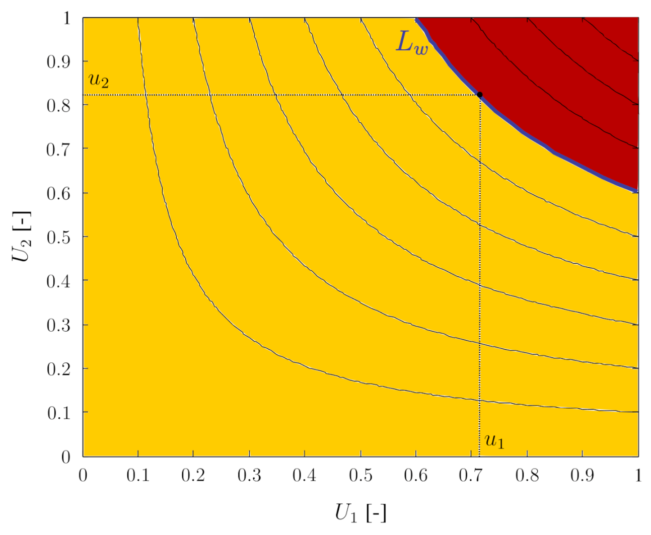
On the basis of the constructed vine copulas, the probability of observing a less severe event can be derived. Suppose for reasons of simplicity that a drought event is only described by two characteristics. Hence, their dependence is described by means of a bivariate copula. For each copula, level curves can be defined as the set of couples that have the same value in the copula:
with . Figure 4 schematically represents the level curves of a copula. Furthermore, the set defined as:
is then the region in below the level curve . This region is indicated in yellow in Figure 4. With this region, a probability is associated:
Hence, is the cumulative distribution function of the random variable . In practice, for an ongoing drought event with values of the characteristics, and corresponding transformed values , its value can be calculated, and can be interpreted as the probability of observing a subcritical or less severe event than the given event. By extending this reasoning to vine copulas, the probability of observing a less severe drought event than an ongoing drought event can be calculated on the basis of the value in the joint cumulative distribution function values of the drought characteristics:
For an ongoing drought event, given its characteristics and corresponding transformed values , its value can be calculated, and the probability of observing a less severe drought event is then calculated as the probability to obtain smaller values than :
In order to obtain the probability of observing a worse or supercritical drought event, can be used, i.e., the probability of observing an event for which the value in the copula is higher than the value of the currently observed event. The region associated with the probability of observing a supercritical event for a bivariate copula is conceptually indicated in red in Figure 4. By calculating the value of for an ongoing drought event, one is thus able to estimate its severity on the basis of the dependence between its three characteristics, affected area, duration and intensity. In this way, can be used to express the drought severity. Note that drought events with the same value of are situated on the same level curve of the copula . These drought events will hence have different values of the characteristics, yet as they have the same value of w and , they have an equal probability of observing a less severe or subcritical event.
As a means to construct the vine copula, copulas from the Gaussian, the t, the Frank, the Clayton and the Gumbel families were employed to search for the most suitable bivariate copulas in the vine copula. These copula families are well known and have already proven their usefulness in hydrological studies [32]. To select the best fitting bivariate copulas, the Akaike Information Criterion (AIC) was used. The structure of the vine copula was selected as the maximum spanning tree [33] with edge weights given by the values of Kendall’s tau (), i.e., a measure describing the dependence between two variables connected by the edges. Furthermore, the White goodness-of-fit test [34] was carried out to further test whether the dependence in the data is well described by means of the selected copulas. The R-package VineCopula [35] was used to identify the vine copula and perform the White goodness-of-fit test.
Before constructing the marginal cumulative distribution functions, noise that is several orders of magnitude smaller than the smallest non-zero difference between any two values in the series, was added to the characteristics as to prevent the occurrence of tied ranks, which is to be avoided when fitting copulas to data [36]. As explained before, the marginal cumulative distributions were used to transform each of the drought characteristics to such that copulas can be fitted. Table 2 shows the structure of the vine copula and the copula families selected for describing the dependence of the drought characteristics. In this table, the first variable refers to affected area, the second to the duration and the third to intensity. Furthermore, the values of Kendall’s tau are also listed. A positive (resp. negative) value reflects a positive (resp. negative) dependence. A value of zero indicates independence. These values show that drought duration is positively associated with drought intensity and affected area. The longer the duration, the more intense the drought event and the larger its affected area. The conditioned variables also show a positive, yet less strong dependence. The White goodness-of-fit test yields a p-value of , which indicates that the dependence structure can be described by these copula families. Table 2 furthermore shows that the vine structure corresponding to the maximum spanning tree uses drought duration as the conditioning variable.
On the basis of the determined vine copulas, the values in the cumulative probability distribution can be determined. To do so, these values were numerically estimated by means of the algorithm by Salvadori et al. [37]. For each of 10,000 samples , the corresponding value is calculated. The value in the cumulative distribution function is then estimated as the percentage of samples that have a CDF value below that of the ongoing drought event. Table 3 lists the probability of observing a less severe drought event for the characteristics of the ongoing drought event, as experienced on 2 November 2012, and for its characteristics upon completion of the event. It is observed that for the ongoing drought event, these values are larger than 0.9, showing that there is a large probability that drought events are less severe. This indicates that the ongoing event is already quite severe compared to the other observed events in the database. As to be expected, the value in the cumulative distribution function increases as the event advances (see Table 3), although for the ongoing event this increase is minimal as the event is near its end at 2 November 2012. Also, in this case, the calculation of the probability to obtain subcritical events is best performed regularly while the event is evolving, as the characteristics of the ongoing drought event will change and measures to be taken might have to be readjusted.
As the general public understands the concept of chance, using the derived probability in communicating about an ongoing drought event may help laymen to assess its severity and the rareness of its occurrence. Especially when very low chances are reported of having a more severe drought, people may become more inclined to follow water saving guidelines issued by the governments or water managers. Furthermore, it should be possible to define the return period of the ongoing drought event based on the derived probability. This value, which provides an average time between two drought events with a severity that is at least equal to that of the ongoing event, may further help laymen to understand the rareness of the situation they face. However, since various definitions of return period are available in a multivariate context [38], further research is needed to pinpoint which type of return period can best be used for communication purposes.
However, one should be careful when using probabilities, especially in view of climate change, as droughts are expected to occur more often. As such, the probability distribution that corresponds to the current droughts may change in time, causing also the probabilities of occurrence to change (and thus also the corresponding return periods). Yet, the analysis described in this paper assumes that the different events belong to the same distribution, and that the stationarity assumption is fulfilled. To the best of our knowledge, no statistical tools are yet available to account for the non-stationarity induced by climate change, while greatly needed. One way for coping with this, while still using the classical stationarity-assuming tools, is to only include droughts of a recent past (e.g., the previous 30 year), assuming that within the time frame used, the climate can be considered as near-stationary. Of course, the shorter the time frame, the smaller the impact of the stationarity assumption. However, shorter time frames result in less droughts, which may therefore lead to an underfitting of the multivariate distribution. Finding the optimum length of such time frame requires further research.
5. Conclusions
In view of the management of a drought, it is crucial that water managers as well as the broad public are aware of the severity of the ongoing event. Communication plays a crucial role in creating this awareness. Although several drought indices have been proposed in literature, they cannot be used in drought communication as they are generally not understood by laymen. Referring to historically similar droughts can help people to assess the severity of the ongoing event. Alternatively, expressing the chance that a drought event could be worse than the ongoing one also provides insight in its severity, since this concept is easily understood by most people.
This paper lays out the methodology needed to provide a solution to either option. To do so, drought events in mainland Australia, as identified by Vernieuwe et al. [4] were used, along with the affected area, duration and intensity as drought characteristics. These spatio-temporal drought events were derived from a 35-year GLEAM data set of daily soil moisture at a 0.25° spatial resolution [20].
It is illustrated that, on the basis of the characteristics of an identified drought event, the database of historical drought events can be queried such that similar drought events can be identified. Besides using this information to increase the public awareness, this query can also help water managers to incorporate lessons learnt from the past in order to better cope with the ongoing drought event, and as such anticipate the future.
The second application unfolded in this paper addresses the question on the chance of the occurrence of a more severe drought. To that end, a probabilistic model that makes use of a vine copula to account for the dependence between drought intensity, duration and extent, can be used in order to determine the probability to experience a more severe or a supercritical event and hence conclusions about the severity of the event can be drawn.
Author Contributions
Conceptualisation, H.V., B.D.B., and N.E.C.V.; methodology, H.V., B.D.B., and N.E.C.V.; formal analysis and investigation, H.V.; resources, B.D.B. and N.E.C.V.; writing—original draft preparation, H.V.; writing—review and editing, H.V., B.D.B., and N.E.C.V.; supervision, B.D.B. and N.E.C.V.; funding acquisition and project administration, B.D.B. and N.E.C.V. All authors have read and agreed to the published version of the manuscript.
Funding
This work was funded by the Belgian Science Policy, project SR/00/302, and by FWO, grant number G.0039.18N.
Institutional Review Board Statement
Not applicable.
Informed Consent Statement
Not applicable.
Data Availability Statement
Data sharing not applicable.
Acknowledgments
We thank Marcus Enenkel for a fruitful discussion on drought management which laid the basis for this research.
Conflicts of Interest
The authors declare no conflict of interest.
References
- Mishra, A.K.; Singh, V.P. A review of drought concepts. J. Hydrol. 2010, 391, 202–216. [Google Scholar] [CrossRef]
- Tallaksen, L.M.; Van Lanen, H.A.J. Drought as a natural hazard: Introduction. In Hydrological Drought Processes and Estimation Methods for Streamflow and Groundwater; Developments in Water Science; Tallaksen, L.M., Van Lanen, H.A.M., Eds.; Elsevier: Amsterdam, The Netherlands, 2004; pp. 3–17. [Google Scholar]
- American Meteorological Society. Statement on meteorological drought. Bull. Am. Meteorol. Soc. 2004, 85, 771–773. [Google Scholar]
- Vernieuwe, H.; De Baets, B.; Verhoest, N.E.C. A mathematical morphology approach to the identification of drought events in space and time. Int. J. Climatol. 2020, 40, 530–543. [Google Scholar] [CrossRef] [Green Version]
- Sheffield, J.; Andreadis, K.M.; Wood, E.F.; Lettenmaier, D.P. Global and continental drought in the second half of the twentieth century: Severity–Area–Duration analysis and temporal variability of large-scale events. J. Clim. 2009, 22, 1962–1981. [Google Scholar] [CrossRef]
- Halwatura, D.; Lechner, A.M.; Arnold, S. Drought severity–duration–frequency curves: A foundation for risk assessment and planning tool for ecosystem establishment in post-mining landscapes. Hydrol. Earth Syst. Sci. 2015, 19, 1069–1091. [Google Scholar] [CrossRef] [Green Version]
- Pham, M.T.; Vernieuwe, H.; De Baets, B.; Verhoest, N.E.C. A coupled stochastic rainfall-evapotranspiration model for hydrological impact analysis. Hydrol. Earth Syst. Sci. 2018, 22, 1263–1283. [Google Scholar] [CrossRef] [Green Version]
- Salvadori, G.; De Michele, C. On the use of copulas in hydrology: Theory and practice. J. Hydrol. Eng. 2007, 12, 369–380. [Google Scholar] [CrossRef]
- Serinaldi, F.; Bonaccosro, B.; Cancelliere, A.; Grimaldi, S. Probabilistic characteriation of drought properties through copulas. Phys. Chem. Earth 2009, 34, 596–605. [Google Scholar] [CrossRef]
- Song, S.; Singh, V.P. Meta-elliptical copulas for drought frequency analysis of periodic hydrologic data. Stoch. Environ. Res. Risk Assess. 2010, 24, 245–444. [Google Scholar] [CrossRef]
- Vandenberghe, S. Copula-Based Models for Generating Design Rainfall. Ph.D. Thesis, Ghent University, Gent, Belgium, 2012. [Google Scholar]
- Wong, G.; Lambert, M.G.; Leonard, M.; Metcalfe, A.V. Drought analysis using trivariate copulas conditional on climatic states. J. Hydrol. Eng. 2010, 15, 129–141. [Google Scholar] [CrossRef]
- Aas, K.; Czado, C.; Frigessi, A.; Bakken, H. Pair-copula constructions of multiple dependence. Insur. Math. Econ. 2009, 44, 182–198. [Google Scholar] [CrossRef] [Green Version]
- Bedford, T.; Cooke, R.M. Probability density decomposition for conditionally dependent random variables modeled by vines. Ann. Math. Artif. Intell. 2001, 32, 245–268. [Google Scholar] [CrossRef]
- Bedford, T.; Cooke, R.M. Vines—A new graphical model for dependent random variables. Ann. Stat. 2002, 30, 1031–1068. [Google Scholar] [CrossRef]
- Erhardt, T.M.; Czado, C. Standardized drought indices: A novel univariate and multivariate approach. J. R. Stat. Soc. Ser. C: Appl. Stat. 2018, 67, 643–664. [Google Scholar] [CrossRef] [Green Version]
- Hao, Z.C.; Singh, V.P. Review of dependence modeling in hydrology and water resources. Prog. Phys. Geogr. 2016, 40, 549–578. [Google Scholar] [CrossRef]
- Pham, M.T.; Vernieuwe, H.; De Baets, B.; Willems, P.; Verhoest, N.E.C. Stochastic simulation of precipitation-consistent daily reference evapotranspiration using vine copulas. Stoch. Environ. Res. Risk Assess. 2016, 30, 2197–2214. [Google Scholar] [CrossRef] [Green Version]
- Shafaei, M.; Fakheri-Fard, A.; Dinpanshoh, Y.; Mirabbasi, R.; De Michele, C. Modeling flood event characteristics using D-vine structures. Theor. Appl. Climatol. 2017, 130, 713–724. [Google Scholar] [CrossRef]
- Martens, B.; Miralles, D.G.; Lievens, H.; van der Schalie, R.; de Jeu, R.A.M.; Fernández-Prieto, D.; Beck, H.E.; Dorigo, W.A.; Verhoest, N.E.C. GLEAM v3: Satellite-based land evaporation and root-zone soil moisture. Geosci. Model Dev. 2017, 10, 1903–1925. [Google Scholar] [CrossRef] [Green Version]
- Miralles, D.G.; Holmes, T.R.H.; De Jeu, R.A.M.; Gash, J.H.; Meesters, A.G.C.A.; Dolman, A.J. Global land-surface evaporation estimated from satellite-based observations. Hydrol. Earth Syst. Sci. 2011, 15, 453–469. [Google Scholar] [CrossRef] [Green Version]
- McCarthy, J.J.; Canziani, O.F.; Leary, N.A.; Dokken, D.J.; White, K.S. Working Group II: Impacts, Adaptation, and Vulnerability; Technical Report; The Press Syndicate of the University of Cambridge: Cambridge, UK, 2001. [Google Scholar]
- Sheffield, J.; Goteti, G.; Wen, F.; Wood, E.F. A simulated soil moisture based drought analysis for the United States. J. Geophys. Res. 2004, 109, D24108. [Google Scholar] [CrossRef]
- Sheffield, J.; Wood, E.F. Characteristics of global and regional drought, 1950–2000: An analysis of soil moisture data from off-line simulation of the terrestrial hydrological cycle. J. Geophys. Res. 2007, 112, D17115. [Google Scholar] [CrossRef] [Green Version]
- Serra, J. Introduction to mathematical morphology. Comput. Vision Graph. Image Process. 1986, 35, 283–305. [Google Scholar] [CrossRef]
- Haralick, R.M.; Sternberg, S.R.; Zhuang, X. Image analysis using mathematical morphology. IEEE Trans. Pattern Anal. Mach. 1987, 9, 532–550. [Google Scholar] [CrossRef] [PubMed]
- Sklar, A. Fonctions de répartition á n dimensions et leurs marges. Publ. Inst. Stat. Univ. Paris 1959, 8, 229–231. [Google Scholar]
- Nelsen, R.B. An introduction to copulas. In Lecture Notes in Statistics; Bickel, P., Diggle, P., Fienberg, S., Krickeberg, K., Olking, I., Wermuth, N., Zeger, S., Eds.; Springer: New York, NY, USA, 2006; p. 216. ISBN 978-1-4419-2109-3. [Google Scholar]
- Pircalabu, A.; Jung, J. A mixed C-vine copula model for hedging price and volumetric risk in wind power trading. Quant. Financ. 2017, 17, 1583–1600. [Google Scholar] [CrossRef]
- Zhang, D.L. Vine copulas and applications to the European Union sovereign debt analysis. Int. Rev. Financ. Anal. 2014, 36, 46–56. [Google Scholar] [CrossRef] [Green Version]
- Al Janabi, M.A.M.; Hernandez, J.A.; Berger, T.; Nguyen, D.K. Multivariate dependence and portfolio optimization algorithms under illiquid market scenarios. Eur. J. Oper. Res. 2017, 259, 1121–1131. [Google Scholar] [CrossRef] [Green Version]
- Sadegh, M.; Ragno, E.; AghaKouchak, A. Multivariate copula analysis toolbox (MvCAT): Describing dependence and underlying uncertainty using a Bayesian framework. Water Resour. Res. 2017, 53, 5166–5183. [Google Scholar] [CrossRef]
- Dissmann, J.; Brechmann, E.C.; Czado, C.; Kurowicka, D. Selecting and estimating regular vine copulae and application to financial returns. Comput. Stat. Data Anal. 2013, 59, 52–69. [Google Scholar] [CrossRef] [Green Version]
- Schepsmeier, U. Efficient information based goodness-of-fit tests for vine copula models with fixed margins: A comprehensive review. J. Multivar. Anal. 2015, 138, 34–52. [Google Scholar] [CrossRef]
- Schepsmeier, U.; Stoeber, J.; Brechmann, E.C.; Graeler, B.; Nagler, T.; Erhardt, T. VineCopula: Statistical Inference of Vine Copulas. R Package Version 2.1.4. 2018. Available online: https://CRAN.R-project.org/package=VineCopula (accessed on 26 February 2021).
- Vandenberghe, S.; Verhoest, N.E.C.; De Baets, B. Fitting bivariate copulas to the dependence structure between storm characteristics: A detailed analysis based on 105 year 10 min rainfall. Water Resour. Res. 2010, 46, W01512. [Google Scholar] [CrossRef]
- Salvadori, G.; De Michele, C.; Durante, F. On the return period and design in a multivariate framework. Hydrol. Earth Syst. Sci. 2011, 15, 3293–3305. [Google Scholar] [CrossRef] [Green Version]
- Gräler, B.; van den Berg, M.J.; Vandenberghe, S.; Petroselli, A.; Grimaldi, S.; De Baets, B.; Verhoest, N.E.C. Multivariate return periods in hydrology: A critical and practical review focusing on synthetic design hydrograph estimation. Hydrol. Earth Syst. Sci. 2013, 17, 1281–1296. [Google Scholar] [CrossRef] [Green Version]
Figure 1.
Drought events occurring, on 2 November 2012 in Australia displayed in the Lambert Azimuthal Equal Area coordinate system with a resolution of 27.442 km × 29.079 km. The three different drought events are given different colors.
Figure 1.
Drought events occurring, on 2 November 2012 in Australia displayed in the Lambert Azimuthal Equal Area coordinate system with a resolution of 27.442 km × 29.079 km. The three different drought events are given different colors.

Figure 2.
Schematic representation of a copula fitted to the marginals and .

Figure 3.
The principle of hierarchical nesting of bivariate copulas in the construction of a three-dimensional vine copula through conditional mixtures.
Figure 3.
The principle of hierarchical nesting of bivariate copulas in the construction of a three-dimensional vine copula through conditional mixtures.

Figure 4.
Level curves (black) of a bivariate copula, the region (yellow) corresponding to the probability of observing a less (subcritical) event and the region (red) corresponding to the probability of observing a worse (supercritical) event than an event located on the blue level curve.
Figure 4.
Level curves (black) of a bivariate copula, the region (yellow) corresponding to the probability of observing a less (subcritical) event and the region (red) corresponding to the probability of observing a worse (supercritical) event than an event located on the blue level curve.


Table 1.
Characteristics of drought event at 2 November 2012, experienced at the location indicated in Figure 1 and characteristics of the three most similar drought events in mainland Australia or that include the location.
Table 1.
Characteristics of drought event at 2 November 2012, experienced at the location indicated in Figure 1 and characteristics of the three most similar drought events in mainland Australia or that include the location.
| Affected Area | Duration | Intensity |
|---|---|---|
| [km2] | [days] | [−] |
| ongoing event | ||
| 59 | ||
| three most similar drought events in mainland Australia | ||
| 88 | ||
| 49 | ||
| 114 | ||
| three most similar drought events at the location indicated in Figure 1 | ||
| 88 | ||
| 49 | ||
| 109 | ||
Table 2.
Copula families, structure of the vine copula and values of Kendall’s tau . Subscripts 1, 2 and 3 respectively indicate affected area, duration and intensity.
Table 2.
Copula families, structure of the vine copula and values of Kendall’s tau . Subscripts 1, 2 and 3 respectively indicate affected area, duration and intensity.
| Copula | Family | |
|---|---|---|
| t-copula | 0.43 | |
| Frank | 0.46 | |
| Gaussian | 0.12 |
Table 3.
Values in the cumulative distribution function of the characteristics of the ongoing drought event as experienced at 2 November 2012 () and of its characteristics upon completion of the event ().
Table 3.
Values in the cumulative distribution function of the characteristics of the ongoing drought event as experienced at 2 November 2012 () and of its characteristics upon completion of the event ().
| 0.9776 | 0.9814 |
Publisher’s Note: MDPI stays neutral with regard to jurisdictional claims in published maps and institutional affiliations. |
© 2021 by the authors. Licensee MDPI, Basel, Switzerland. This article is an open access article distributed under the terms and conditions of the Creative Commons Attribution (CC BY) license (http://creativecommons.org/licenses/by/4.0/).
Share and Cite
MDPI and ACS Style
Vernieuwe, H.; De Baets, B.; Verhoest, N.E.C. Effective Drought Communication: Using the Past to Assess the Present and Anticipate the Future. Water 2021, 13, 714. https://doi.org/10.3390/w13050714
AMA Style
Vernieuwe H, De Baets B, Verhoest NEC. Effective Drought Communication: Using the Past to Assess the Present and Anticipate the Future. Water. 2021; 13(5):714. https://doi.org/10.3390/w13050714
Chicago/Turabian StyleVernieuwe, Hilde, Bernard De Baets, and Niko E. C. Verhoest. 2021. "Effective Drought Communication: Using the Past to Assess the Present and Anticipate the Future" Water 13, no. 5: 714. https://doi.org/10.3390/w13050714
Note that from the first issue of 2016, this journal uses article numbers instead of page numbers. See further details here.