
Impact of Prospective Climate Change Scenarios upon Hydropower Potential of Ethiopia in GERD and GIBE Dams


Politecnico di Milano Dipartimento di Ingegneria Civile e Ambientale, L. da Vinci 32, 20133 Milano, Italy
*
Author to whom correspondence should be addressed.
Water 2021, 13(5), 716; https://doi.org/10.3390/w13050716
Submission received: 29 January 2021
/
Revised: 1 March 2021
/
Accepted: 2 March 2021
/
Published: 6 March 2021
(This article belongs to the Special Issue Impact of River Hydrology on Hydraulic Engineering and Hydropower)
Abstract
:Ethiopia is growing fast, and the country has a dire need of energy. To avoid environmental damages, however, Ethiopia is looking for green energy polices, including hydropower exploitation, with large water availability (i.e., the Blue Nile, the greatest tributary of Nile river). Besides other dams on the Omo river, the GIBE family, Ethiopia is now building the largest hydropower plant of Africa, the GERD (Grand Ethiopian Renaissance Dam), on the Blue Nile river, leading to tensions between Ethiopia, and Egypt, due to potentially conflictive water management. In addition, present and prospective climate change may affect reservoirs’ operation, and this thereby is relevant for downstream water users, population, and environment. Here, we evaluated water management for the GERD, and GIBE III dams, under present, and future hydrological conditions until 2100. We used two models, namely, Poli-Hydro and Poli-Power, to describe (i) hydrological budget, and flow routing and (ii) optimal/maximum hydropower production from the two dams, under unconstrained (i.e., no release downstream besides MIF) and constrained (i.e., with fair release downstream) simulation. We then used climate change scenarios from the reports CMIP5/6 of the Intergovernmental Panel on Climate Change (IPCC) until 2100, to assess future hydropower production. Our results demonstrate that the filling phase of the GERD, particularly critical, have optimal filling time of 5 years or so. Stream flows at GERD could be greater than the present ones (control run CR) at half century (2050–2059), but there could be large decrease at the end of century (2090–2099). Energy production at half century may increase, and then decrease until the end of century. In GIBE III discharges would increase both at half century, and at the end of century, and so would energy production. Constrained, and unconstrained simulation provide in practice similar results, suggesting potential for shared water management in both plants.
1. Introduction
Population of Ethiopia is growing fast, ever increasing the demand of energy for industries and domestic use. To save the environment, Ethiopia is looking for green energy polices, and thus they are properly planning hydropower exploitation. Large hydropower potential is present in the region, given orography, climate and large water availability (i.e., in the Blue Nile, the greatest tributary of Nile river [1,2]).
Ethiopia is presently building the biggest hydropower plant in Africa ever, i.e., the Great Ethiopian Renaissance Dam GERD, on the Blue Nile river. However, prospective operation of such dam increased the tensions between the governments of Ethiopia and Egypt [3]. Other dams were built in the Omo river catchment, in South Ethiopia, including GIBE family, i.e., GIBE I, II, III, the last one to be operative in short, while GIBE I, II are operating fully (Figure 1).
Water management strategies in these systems need to be pursued with an eye upon maximum production/profit, while possibly respecting downstream water requirements, be them for ecological flows (minimum in stream flows MIFs), irrigation, or other needs of downstream population, and environment.
GIBE I plant is used only for hydropower production, with a MIF evaluated from designers of 2 m3 s−1 according to the Ministry of Mines and the Energy Ethiopian Electric Light and Power Authority [4]. GIBE II operates with downstream water from GIBE I, working in practice as a run of river ROR hydropower plant. GERD and GIBE III instead feature large storage capacity, and operation thereby is relevant for downstream water users. In the present literature, some information is available covering hydrology of the Nile and Omo rivers (e.g., [5,6,7,8]), also giving information of climate in the area.
Even, some previous studies on the influence of climate change focused attention upon present changes in runoff (e.g., [9,10,11,12,13,14]).
Overall, the present literature shows that water resources of Ethiopia are highly sensitive to climate change, and interannual variability [15], and water management requires a thorough assessment of the impact of climate change on stream flows [16].
Climate change will impact the availability and seasonality of fresh water, because of the expectedly modified frequency of climate extremes, such as heat waves (e.g., by leading evapotranspiration patterns), meteorological and hydrological droughts, and changes in rainfall patterns [17].
The uncertain availability of water resources may further affect agricultural production, challenging the socio-economic system and competing with energy production. The Intergovernmental Panel on Climate Change IPCC indicated Africa as a most vulnerable continent to climate change and climate variability [18], particularly for countries with economy heavily dependent upon agricultural production, such as Ethiopia [19]. Present, and prospective climate change may specifically affect reservoirs’ operation. Temperature, and possibly precipitation changes, and influence upon the hydrological regime thereby, may affect (either positively or negatively) hydropower production [20,21].
Outside Africa, the impact of climate change on hydropower have been explored, e.g., by Li et al. [22], examining the effect on the Pearl River, China. They highlight a greater vulnerability of the hydroelectric system, particularly in the drier years that are not compensated by the surplus in the more wet years, leading a general decrease in efficiency of the system. Tarroja et al. [23] instead studied the hydropower generation under climate change in highly renewable electric grid configuration, and they found a possible future decrease on production of energy despite the increase in flow which, instead, causes spillage from the reservoirs.
The aim of this study is to describe potential changes in hydropower production for GERD and GIBE III dams, under future hydrological conditions until 2100.
First, based on a dependable and unique hydrological data set [24] gathered during 1960–2019, we set up the model Poli-Hydro, able to mimic hydrological flow formation in several areas hitherto (see for further details e.g., [25,26,27,28]).
We used Poli-Hydro (see [25,26,27,28]) to describe daily hydrological budget and flow routing of upstream catchments and Poli-Power to mimic optimal daily hydropower production from the dams.
Poli-Hydro was used to simulate hydrological behavior during a calibration period (CP) 1965–1988. Then, we simulated stream flows and potential hydropower production during a control run (CR) period 2010–2019. Hydropower production is optimized using a tool called Poli-Power [26,28], which maximizes the revenues for plants’ manager under given hydrological regimes.
We considered here two operation scenarios, namely, (i) constrained, i.e., with proper release downstream, to supply irrigation and Turkana lake evaporation (mostly laid in Kenya) and (ii) unconstrained, i.e., with no release downstream besides MIF.
We then used climate change scenarios of IPCC from reports CMIP5/6 (3 models of each CMIP, with RCP and SSP scenarios, 21 scenarios overall, properly downscaled), until 2100 as inputs to the Poli-Hydro model, to generate daily future series of stream flows, to subsequently assess hydropower production under new regulation strategies.
The paper is organized as follows. In the section “Case study,” we present the areas of interest and main characteristics of the studied hydropower plants. In the section “Data Base,” we describe the available information used here for calibration of the models and, in general, for the study. In “Methods” section, we depict the main traits of our models. In the section “Results,” we report models’ performance, future flow regimes, and hydropower production. In the sections “Discussion” and “Conclusions,” we comment on our results against uncertain projections of future climate, we provide limitations and outlooks, and we summarize some conclusions of our study.
2. Case Study Area
2.1. GERD
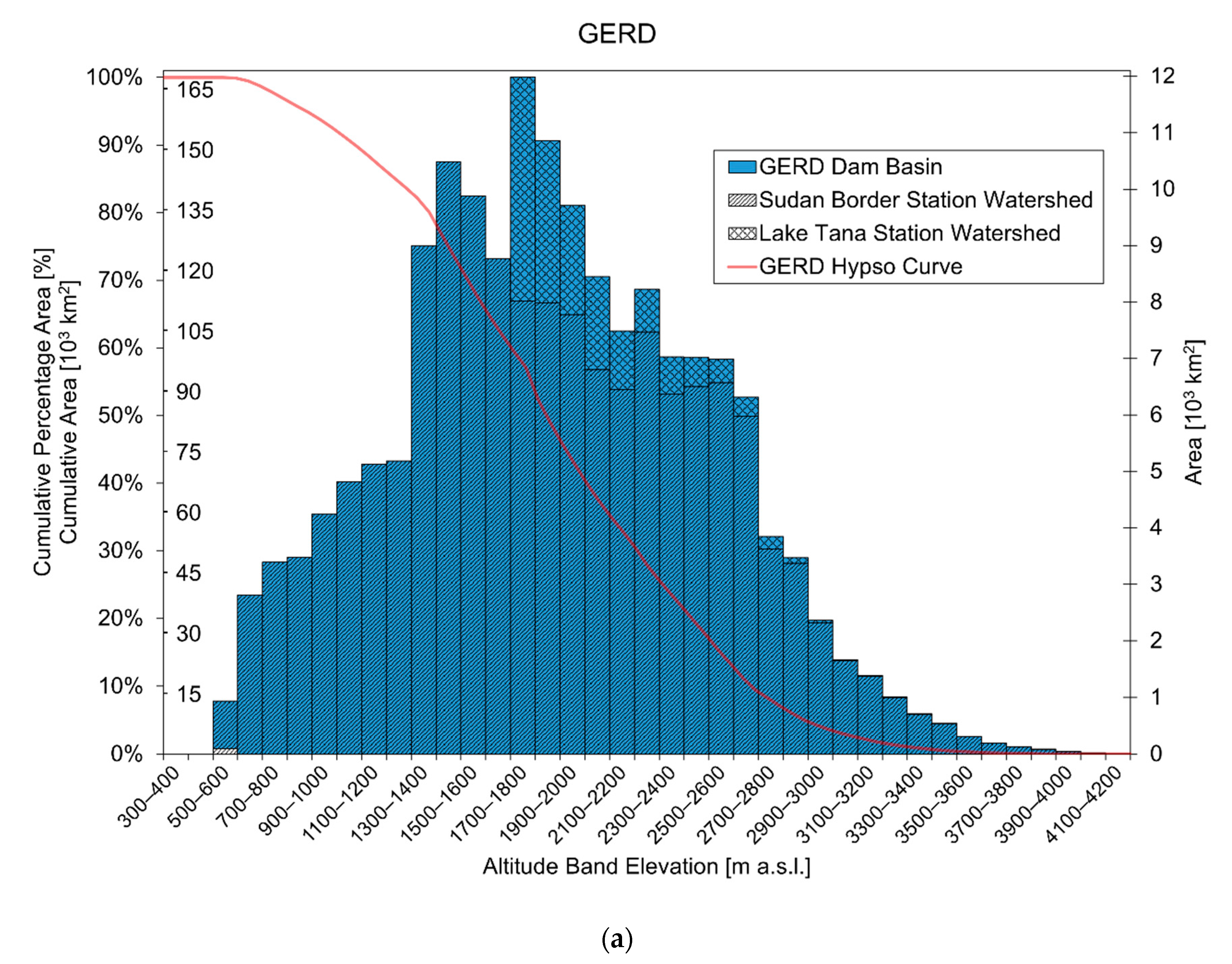
GERD dam will be the largest dam build in Africa hitherto. The installed power will be 6000 MW, with an annual production of 15.7 TWh. The dam’s crest will be at 675 m a.s.l., and the maximum operation level will be 640 m a.s.l. The lake level will change between 590 and 640 m a.s.l. The reservoir volume will be 74 Gm3, with operation volume of 59 Gm3. The maximum turbine discharge is 4305 m3 s−1, split between 16 turbines of 375 MW each (as described by [3,29,30]). Average annual temperature of the Blue Nile catchment (168 × 103 km2, the hypsographic curve is presented in Figure 2) closed at the dam during 1965–1988 was +12 °C, with a minimum of +3 °C and maximum of +18 °C. The warmest period is March–August. Mean annual precipitation was 1500 mm year−1, with largest rainfall between June and September.
2.2. GIBE I
GIBE I is the first GIBE hydropower plant built on a tributary of the Omo river. The installed power reaches 210 MW. Dam’s height is 40 m, dam’s crest is at 1675 m a.s.l. Reservoir volume is 830 Mm3, with operable volume of 711 Mm3. The maximum turbine discharge is 101.5 m3 s−1 over 3 turbines, 70 MW each [4,31].
The mean basin wide (4040 km2) annual temperature (1965–1988) is +9 °C with a minimum of −5 °C and maximum of +17 °C. The warmest period is April to August. Mean annual precipitation was 1100 mm year−1, with largest rainfall during August to September.
2.3. GIBE II
GIBE II was the second hydropower plant of GIBE family built on the Omo river, downstream of GIBE I. The plant uses the turbine water from GIBE I, plus water from a small trait (80 km2) between GIBE I and GIBE II intake. The water enters in two penstocks, 26 km long, and it is released in Omo river, after a 460–495 m hydraulic jump. The installed power is 420 MW. Dam’s height is 33 m, and dam’s crest is at 1437 m a.s.l. Reservoir volume is 1.3 Mm3, with operable volume of 0.3 Mm3. The maximum turbine discharge is 101.5 m3 s−1 over 4 Pelton turbines, of 105 MW each [31].
2.4. GIBE III
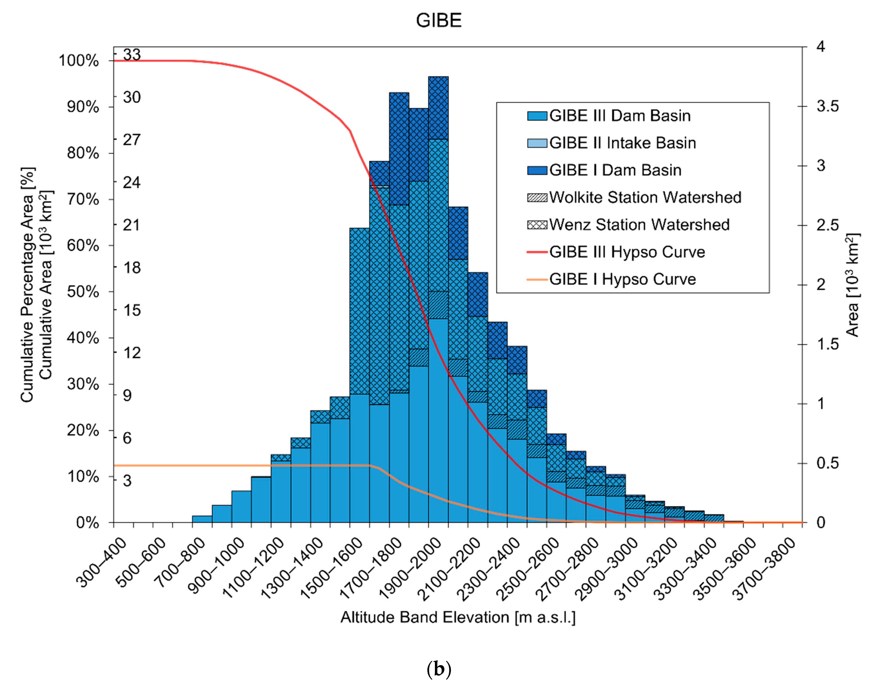
GIBE III is the last plant built on Omo basin insofar. The installed power is 1870 MW, with an annual production of 6500 GWh. Dam’s height is 250 m, dam’s crest being at 896 m a.s.l. Reservoir volume is 11.750 Gm3. The maximum turbine discharge is 950 m3 s−1, distributed on 10 Francis turbines, of 187 MW each [32,33,34].
The mean annual (1965–1988) basin wide (32,500 km2) temperature was +10.5 °C, with minimum of 0 °C and maximum of +16 °C. The warmest period is between March and August. Mean annual precipitation was 1400 mm year−1, with largest rainfall between August and September.
3. Data Base
3.1. Poly-Hydro Model Setup (1965–1988)
The Nile and Omo catchments have different hydrological behavior, so we studied these two regions separately. We used 10 meteorological stations (precipitation P and maximum, minimum, and mean temperatures Tmax, Tmin, and Tmean) from the National Oceanic and Atmospheric Administration (NOAA) [24], covering the study area. Unfortunately, the data thereby covered 1965–1988. The stations are reported in Table 2. Using the NOAA data, we found a clear linear altitudinal gradient of temperature, but no significant lapse rate of precipitation. Topography is described using a Digital Elevation Model (DEM) from NASA Earth Data [35], with a spatial resolution of 6 km, used also for semi-distributed simulation, as a good trade-off between the required computational time and a good depiction of hydrological processes. Monthly discharges information’s were retrieved from “The Global Runoff Data Centre” [36], at the stations in Figure 1, and reported in Table 3. We used soil cover from Copernicus Global Land Service (CGLS) [37]. The Poli-Hydro model uses a maximum soil moisture Wmax, calculated as from the Curve Number (CN) method, so we converted the CGLS in a CN(Wmax) map.
3.2. Hydropower Production and Price
No specific data for hydropower production or prices were made available from the Ministry of Water Irrigation and Electricity of Ethiopia. Accordingly, we built a reference hydropower scenario for all hydropower plants, in a reference decade 2010–2019, which we call here Control Run (CR). Historical energy production data are not available from any source that we know of (GIBE I and GIBE III). GERD is not operating yet. One way to make a comparison over different periods was therefore to use a unique reference or control run period (CR). In Ethiopia, there is no free market, and a fixed energy price is laid out from the government.
Between Ethiopia and neighbor countries, there are tensions, especially with Egypt, because of the construction of GERD, which could influence largely the hydrological regime of the Blue Nile river. In consideration of potential future agreements and of shared cooperation between States, we hypothesized here two scenarios for water operation for both dams, GERD and GIBE III. All plants are built to fully operate downstream water, i.e., the water used for hydropower is released immediately downstream of the dams.
For GERD, the unconstrained scenario, called here as No Release Scenario (S1), is with no minimum water release. Optimization of hydropower production is pursued without any constraints for release downstream. The second, constrained scenario, is called Environmental Release Scenario (S2) and assumes water wise cooperation, with a minimum (monthly) discharge delivered downstream (after hydropower use) for irrigation purposes, in Egypt and Sudan. The water demand for downstream country was evaluated using the ACQUASTAT Database [38] from FAO, where the different components for agricultural need were retrieved and aggregated to define an overall water demand. Accordingly, boundary conditions change over the year.
For GIBE III, we considered that Omo river is the greatest tributary of Turkana lake. This is an endorheic lake with high evaporation, mostly laid in Kenya. Therefore, the less water flows within the Omo river, the larger losses occur in the Turkana lake, with large ecological implications. We hypothesized a first scenario, No Release Scenario (S1), with a minimum water release MIF = 25 m3 s−1, as from the original dam’s design [32,33], and no water for Turkana lake. Second, we calculated the mean annual evaporation volume from the lake, and we created a scenario called Environmental Release Scenario (S2), including a proper release during flood period (July–September), to supply the Turkana lake properly (i.e., by calculation of losses from evaporation at a monthly scale retrieved from [39], where an analysis of the different flow and impact was carried out).
3.3. Climate Projections (2018–2100)
To project forward hydrology, and thence hydropower production in the reservoirs, we used mean daily temperature, and precipitation scenarios from CMIP5 and CMIP6 of the IPCC [40,41]. We used the outputs of three General Circulation Models, namely EC-Earth (European Consortium Earth system model, version 2 for CMIP5 [42] and version 3 for CMIP6 [43]), CCSM4 (Community System Model, version 4 for CMIP5 [44]), CESM2 (Community Earth System Model, version 2 for CMIP6 [45]), and MPI-ESM (European Center Hamburg Model, with ECHAM version 6.0 for CMIP5 [46] and version 6.3 for CMIP6 [47]). These models were chosen based upon former studies, indicating an acceptable coherence with local temperature and precipitation data [48,49]. Accordingly, we added the new models from the same families, used in the CMIP6 to explore scenarios variability and uncertainty.
For CMIP5, we used three Representative Concentration Pathways (RCP) [50] that are scenarios of greenhouse gasses concentration trajectories. We used RCP 2.6, a most optimistic scenario, with a +1 °C increase of the mean global temperature at the end of 21st century; RCP 4.5 (+2.2 °C); and RCP 8.5 (+3.7 °C). In CMIP6, Shared Socioeconomic Pathways [51] have been introduced, a combination between CO2 and socioeconomic scenarios and projected socioeconomic global changes until 2100. We used SSP1 2.6, which projects a temperature jump of +2 °C (vs. historical baseline) within 2100 and an increase of forest cover. The SSP2 4.5 uses RCP4.5 and moderate land use. The SSP3 7.0 represents a medium-high increase of emission and intense land use; this scenario was implemented to fill the gap present in the RCP scenarios. The last scenario is SSP5 8.5, projecting large economy growth and emissions, with less attention paid to the environment. Overall, due the combination of the models and IPCC scenarios, we could use a total of 21 climate scenarios.
Due to the low spatial resolution of these models (100–200 km in side), statistical downscaling of precipitation and temperature during 1986–2100 was necessary (for further details see [48,49]), which we set up against ground data from NOAA during 1965–1988 [24]. We generated a downscaled GCMs series (precipitation and temperature) for each station. The downscaling procedure resulted into bias-corrected GCMs series, also with proper statistics (i.e., variance in time) with respect to the observed series. This procedure is described elsewhere, and we refer the readers thereby for insights. The so obtained climate series were used as inputs for the Poli-Hydro model, to project forward the hydrological cycle and energy demand at the reservoirs.
4. Methods
4.1. Hydrological Model
We preliminarily studied hydrological regime and hydropower production of all the considered dams. However, we report, here, only the results for GERD and GIBE III, given these two dams are largely the most productive of the four considered (95% of the total hydropower production), and the largest and more important of Ethiopia. Poli-Hydro is a semi-distributed, physically based hydrological model, already validated in several studies [25,26,27,28,52]. Poli-Hydro reproduces different components of the hydrological cycle, and subsequently performs flow routing based upon Nash model [53]. Here, we synthetically depict the model, described fully elsewhere (see e.g., [52]). Poli-Hydro tracks soil water balance for each cell at a daily scale (Wt, the water content at generic day t), see Equation (1), from inputs of precipitation (rainfall R) and outputs of actual evapotranspiration (ET, evaluated as fraction of the potential evapotranspiration ETP), surface (Qs), and sub-surface discharge (Qg). Precipitation in high altitudes is partitioned (rain/snow) using a threshold of mean daily temperature (here, 0 °C). Potential evapotranspiration (also used for lake evaporation) ETP is evaluated using Hargreaves–Samani equation [54]. We evaluated sub-surface discharge, see Equation (2), as a function of terrain permeability (described as potential law using parameter K, the soil saturated conductivity, and k, the ground flow exponent) and water content (W). Surface discharge, see Equation (3), is given from excess of saturation with respect to WMAX, the maximum water content calculated in each cell. Poli-Hydro then performs semi-distributed (i.e., for each cell independently) flow routing based upon a locally tuned (against flow data) Nash model.
4.2. Hydropower Production Model
The model is set up for GIBE III and GERD. Poli-Power optimizes the annual revenue, a behavior expected from hydropower companies, which, however, does not a priori represent the actual regulation of the hydropower plants, which is unknown (and GERD is not operating as yet). We used some hypotheses, namely, (i) all hydropower production is sold on the market, (ii) the reservoir geometry is constant in time (no sediment accumulation, not known hitherto), and (iii) annual prices and consumptions are known. The model works using known inputs of stream flows on a yearly basis (yearly batch operation). Poli-Power inputs are (i) daily stream flows (Q = Qg + Qs), input on an annual basis, (ii) prices (P), and demand of hydropower, (iii) geometry of the reservoir, such as operable volume, maximum and minimum regulation height (H), turbine discharge, and pool-level curves (i.e., water volume vs. height) [26]. We used a constant production efficiency (η), including all expected losses during energy production (i.e., hydraulic losses in the penstocks, in turbines, electric efficiency, etc.). The optimization of revenues, see Equation (4), requires a constraint upon the final annual water volume in the reservoir. Namely, one cannot use (release) all the water volume in the pool, because the residual volume at the end of any year represents a (potential) future revenue in the next year. In Ethiopia, the use of a fixed price requires the creation of a discriminant factor, to address the model towards most convenient production strategies, such as a price behavior in the free market. To do so, we used Poli-Price model [55], to depict hydropower demand (useful also as input to Poli-Power) and subsequently price. We normalized price to unit [26], to obtain a relative priority for production, so being able to force the reservoirs’ operation towards larger production in response to larger demands (and thereby making a larger profit). Poli-Price model builds upon estimates/projections of gross domestic product (GDP) and temperature, and upon proper random factors to account for unexplained fluctuations [56]. The dependence of price from the mean daily temperature is considered, in terms of the power needed for heating/cooling when the temperature exceeds (below or above) from proper thresholds [56]. Poli-Price model is also usable for the purpose of price analysis in the future. The objective function over a given period of optimization is
4.3. Hydrological and Hydropower Projections Until 2100
Using the future climate projections, RCPs and SSPs after proper downscaling, we obtained future projected inputs for the hydrological model until 2100, and thereby future discharges reaching the hydropower plants. We subsequently used the Poli-Power model for optimization of hydropower production. Poli-Price model was set up here using projections of Gross Domestic Product (GDP), of climate based on IPCC scenarios, and uncertainty in the form of random factors, to assess the variability in energy demand, for every day of the year (weekdays, holidays, etc.). Once future hydrology, price, and demand were projected, we could use Poli-Power to maximize future revenues and to evaluate the corresponding energy production, against the CR 2010–2019.
5. Result
5.1. Hydrological Model
Here, we report the tuned values of the Poli-Hydro model parameters and goodness of fit statistics, against monthly discharge data as available. We used NOAA meteorological data, and the available stream flow data to tune the model. Given that there were not enough data for validation/calibration exercise, and considering our focus upon hydropower production rather than upon flow prediction, we only pursued model calibration. The Omo and Blue Nile regions display different hydrological behavior, so we calibrated the model separately. In the Table 4 and Table 5, we report the results of model tuning. Goodness of fit of the model is reported in Table 6. We thereby report monthly NSE (R2), and mean volume error (Bias%), as goodness of fit measures for the available river discharge stations. In Figure 3, we report the observed monthly flows during the calibration period 1965–1988 and the modeled ones at the dam sites.
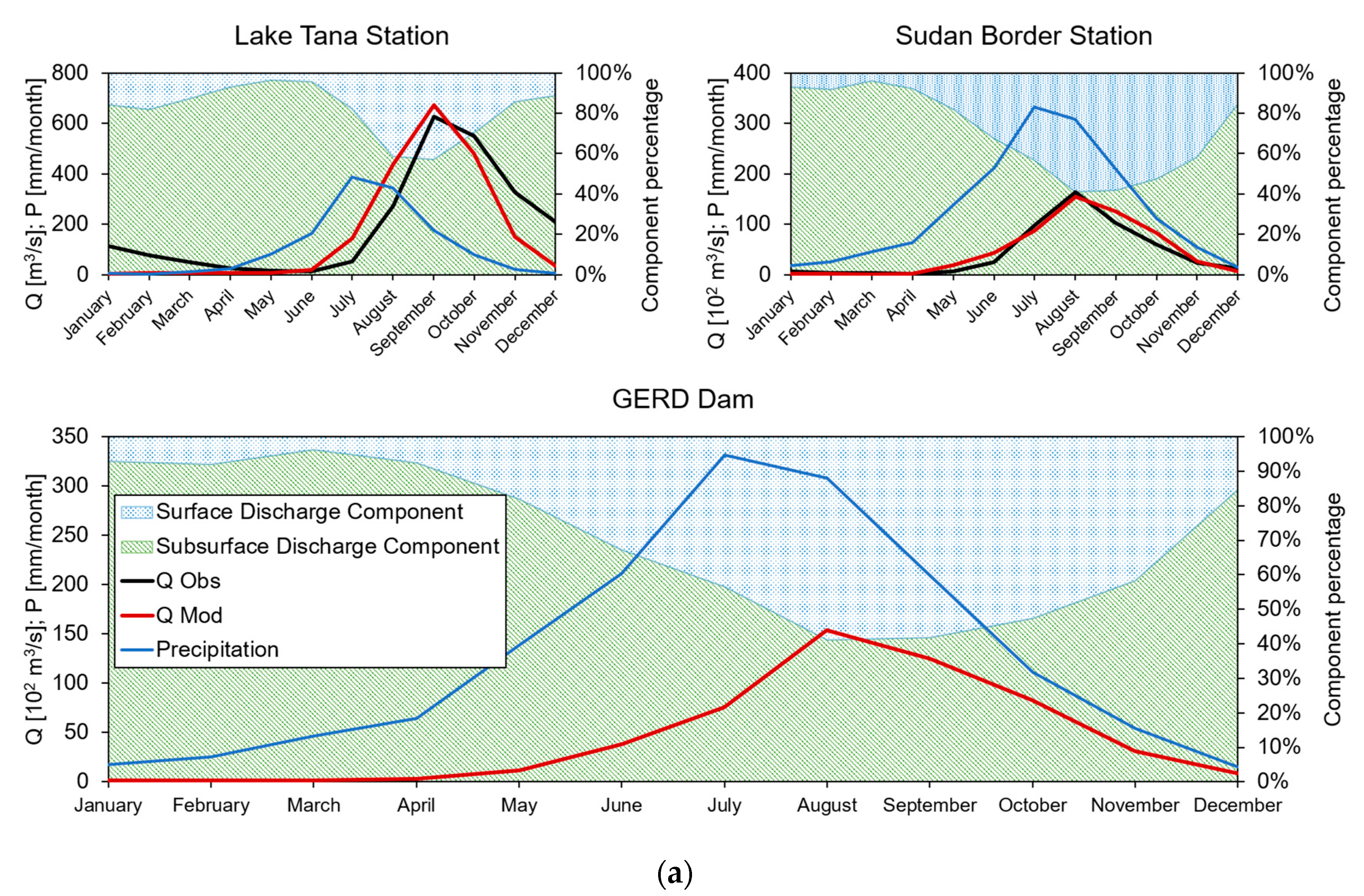
During the calibration period, the estimated mean annual discharge at dam site for the Blue Nile river was 3000 m3 s−1 and for the Omo river it was 605 m3 s−1. The flood period in both rivers is between July and September. Therein, the Nile river would display (daily) discharge as high as 15,000 m3 s−1. The ground water flow covers a smaller share of the total discharge in the case of Blue Nile, but it has more bearing in the Omo river, as seen in Figure 3.
5.2. Hydropower Production
Historical hydropower production is not known here, so we built a reference scenario of hydropower production during 2010–2019 (CR). As reported above, we used two scenarios S1 and S2 for reservoirs’ operation. There were no historical measurements of stream flows during the control run CR (2010–2019), and weather information was sparsely available. Accordingly, we used stream flows as simulated from a mean climate scenario, taken from the IPCC simulations during the CR period. We report separately the results for GERD and GIBE III.
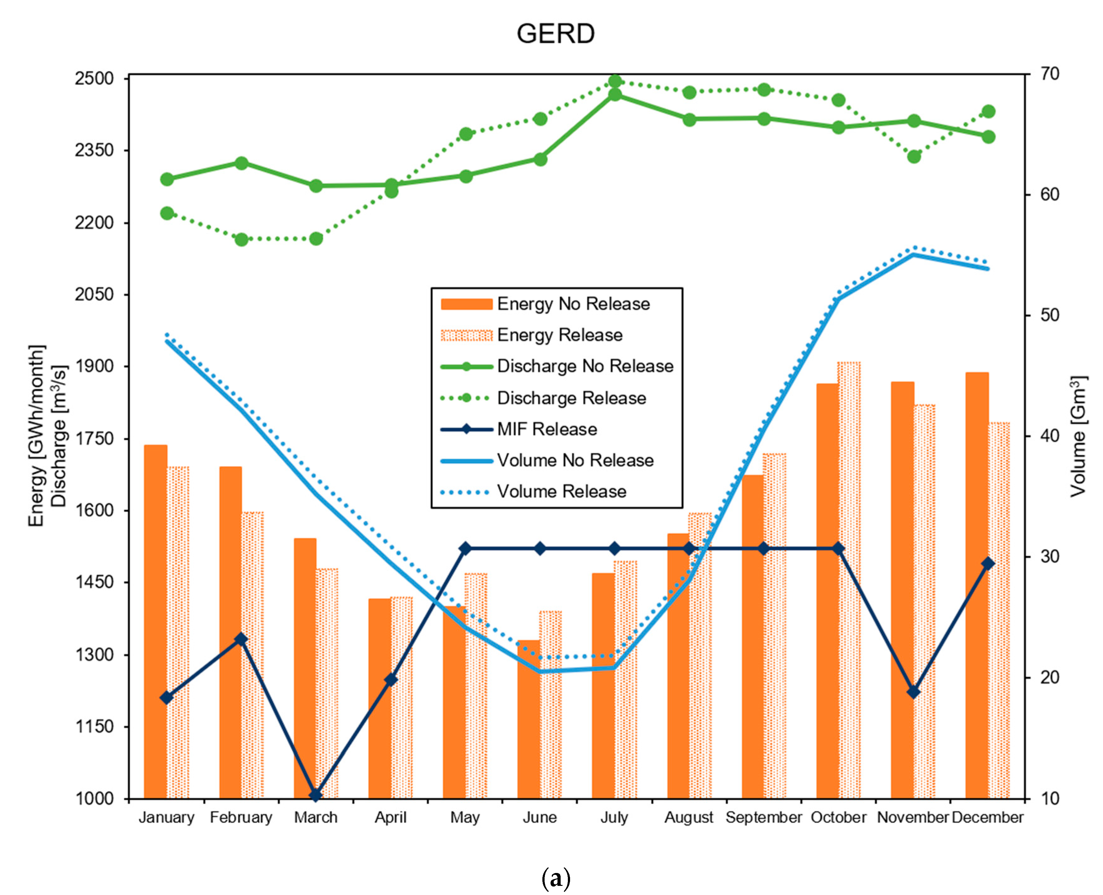
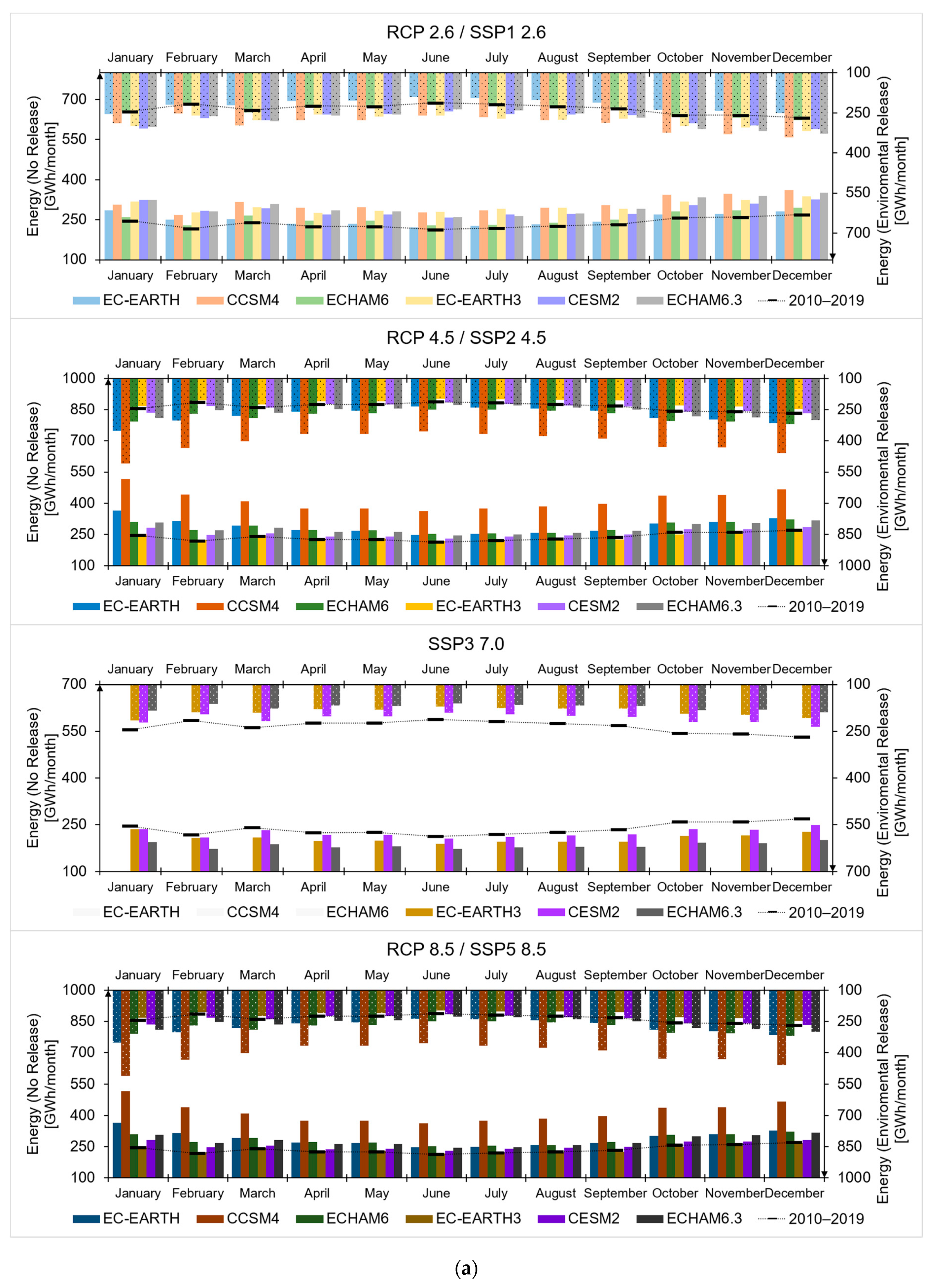
As seen in Figure 4a for GERD plant, water release in option S2 has in practice little influence on, likely due to the very large size of the reservoir. Energy production, for GERD, follows closely stream flow dynamics, with a greater production during flood season, under S2, the energy production is smaller.
Analysis of the discharges in GERD provides on average (2010–2019), Qt = 2358 Qt = 2362 m3 s−1, for S1 and S2, respectively (with ca. +0.2% for S2, small value effect of little influence with respect to release policies). Yearly revenues (relative values) are consequently just little larger for S1 than for S2 (ca. +0.3%).
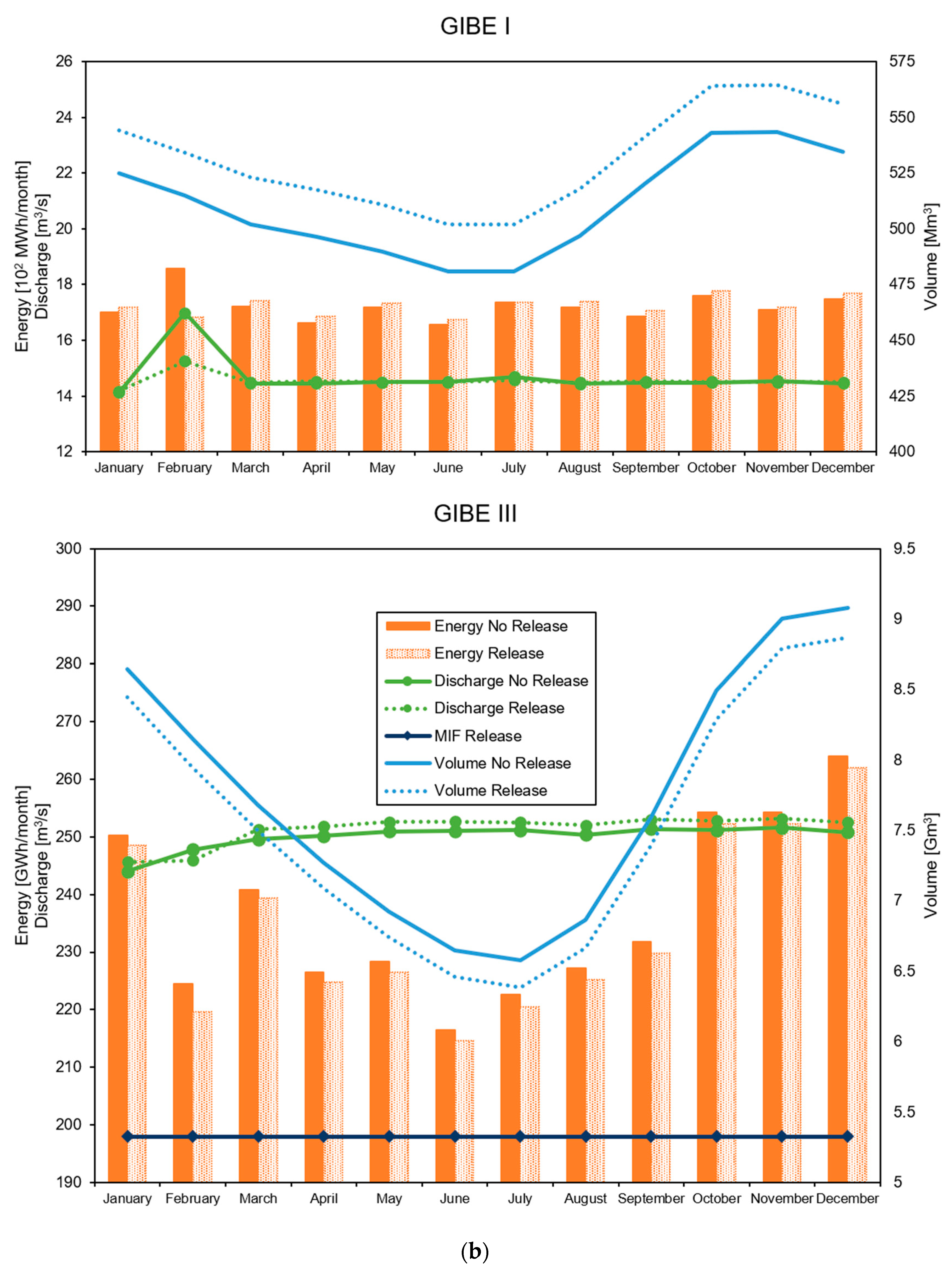
Instead in GIBE III, there is seemingly larger influence from the release conditions, with discharges homogeneously higher in time and with visibly changing stored volumes. If we consider the volumetric fluctuation in the reservoir, it reaches a maximum value of 3.4 Gm3, approximately, 34% of the total active volume.
Under the S2 scenario, energy production is smaller than under S1 scenario. This likely happens because Poli-Power model wants to maximize revenues, and thereby under the S1 scenario, it keeps the lake level high for more profitable periods. This can also be seen in the greater fluctuation of volumes in the S2 scenario, reaching a maximum value of 3.8 Gm3, 39% of the active volume.
Analysis of the hydropower discharges in GIBE III provides on average (2010–2019), Qt = 184 and Qt = 204 m3 s−1, for S1, and S2, respectively (with ca. +8% for S2). Yearly revenues (relative values) are larger for S1 than for S2 (ca. +6%).
5.3. GERD Operation during Filling Phase
Our simulations of GERD operation did not take into account the filling period of the reservoirs (also given that the GERD dam is not operating yet). We indeed started the simulations with an initial condition, given by a reasonable amount of water in the reservoir, greater than the minimum. However, given the very large size of the reservoir, and the relatively fast filling time as expected (ca. 6 years), dam operation during filling period may largely impact stream flows downstream and operation thereby (i.e., along the Nile river, e.g., [3]).
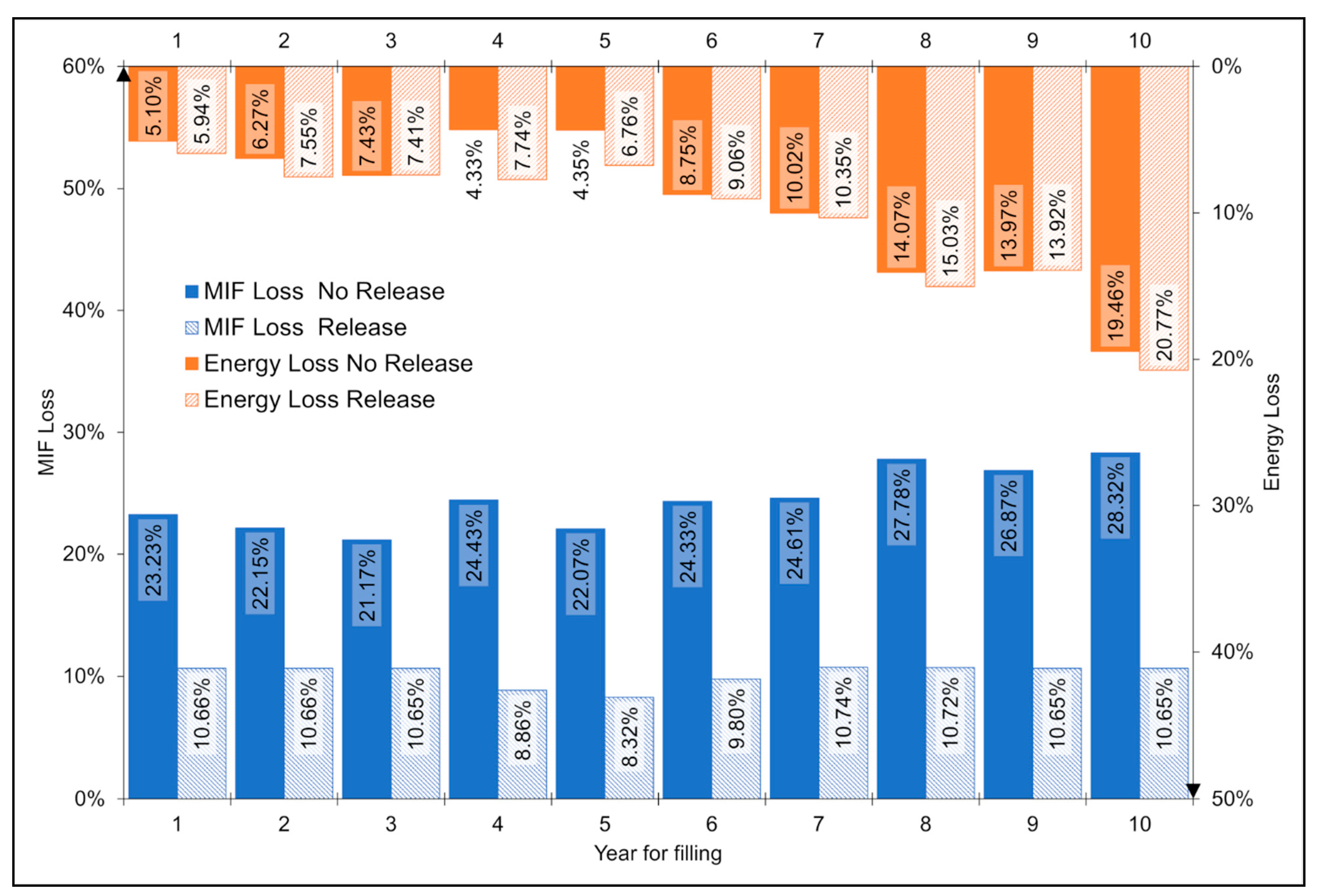
To analyze the effect of filling, we tested reservoir operation during the filling period. Using as input flows the estimated values during 2010–2019, we simulated filling of the reservoir under both conditions S1/S2. We increased the filling period, from 1 to 10 years (i.e., over the whole period with available flow estimates), considering an approximately linear increase of pool volume until filling. After filling, we subsequently hypothesized stationary (on average) operation until the end of the simulation period. We so obtained 10 scenarios of operation during the filling phase (i.e., with filling operation from 1 to 10 years). We then calculated the performance of the reservoirs under the 20 so obtained scenarios (1–10 years filling, S1/S2 option), in terms of (i) power production and (ii) fulfillment of the downstream flow requirements. We compared such performance against a reference scenario, with stationary regulation during 2010–2019 (i.e., with reservoir filled already). In Figure 5, we report the results of our analysis, for both S1/S2 scenarios. We provide the loss of energy and the failure to supply MIF (in terms of MIF volume loss), with respect to the reference scenario, as a function of the filling period duration (1–10 years). These losses are referred to the whole considered period (2010–2019), so the values are comparable.
After a period of relative stability or oscillation (i.e., from 1 to 5 years), one notices a decrease in the energy produced, and the longer the filling period, the larger the loss. Indeed, the longer the filling time, the smaller the volume inside the reservoir. Lower volumes result into lower pool level, and thus into smaller vertical jump for hydropower production. Accordingly, longer filling time results into lower energy production, and increasing energy loss. When one considers the decrease (loss) of downstream flow, this is clearly the highest under the S1 (no release) scenario. Clearly, in lack of constraints for downstream flow release, and in need of gathering water to fill the reservoir, the downstream flow release decreases the most. Under the S2 scenario (fair release), albeit rapid filling is necessary, still some water needs to be released downstream (and used for hydropower), and thereby the MIF loss is lower.
One can spot a clear minimum of energy loss for a period of 4–5 years for filling, under S1 scenario, and a less clear region of minimum for 1–5 years under S2 scenario. Losses in downstream flows seem less variable in the face of filling time.
Periods longer than 6–7 years, however, seemingly provide spoiling of the performance for energy and downstream release, under all scenarios.
5.4. Future Climate of the Area
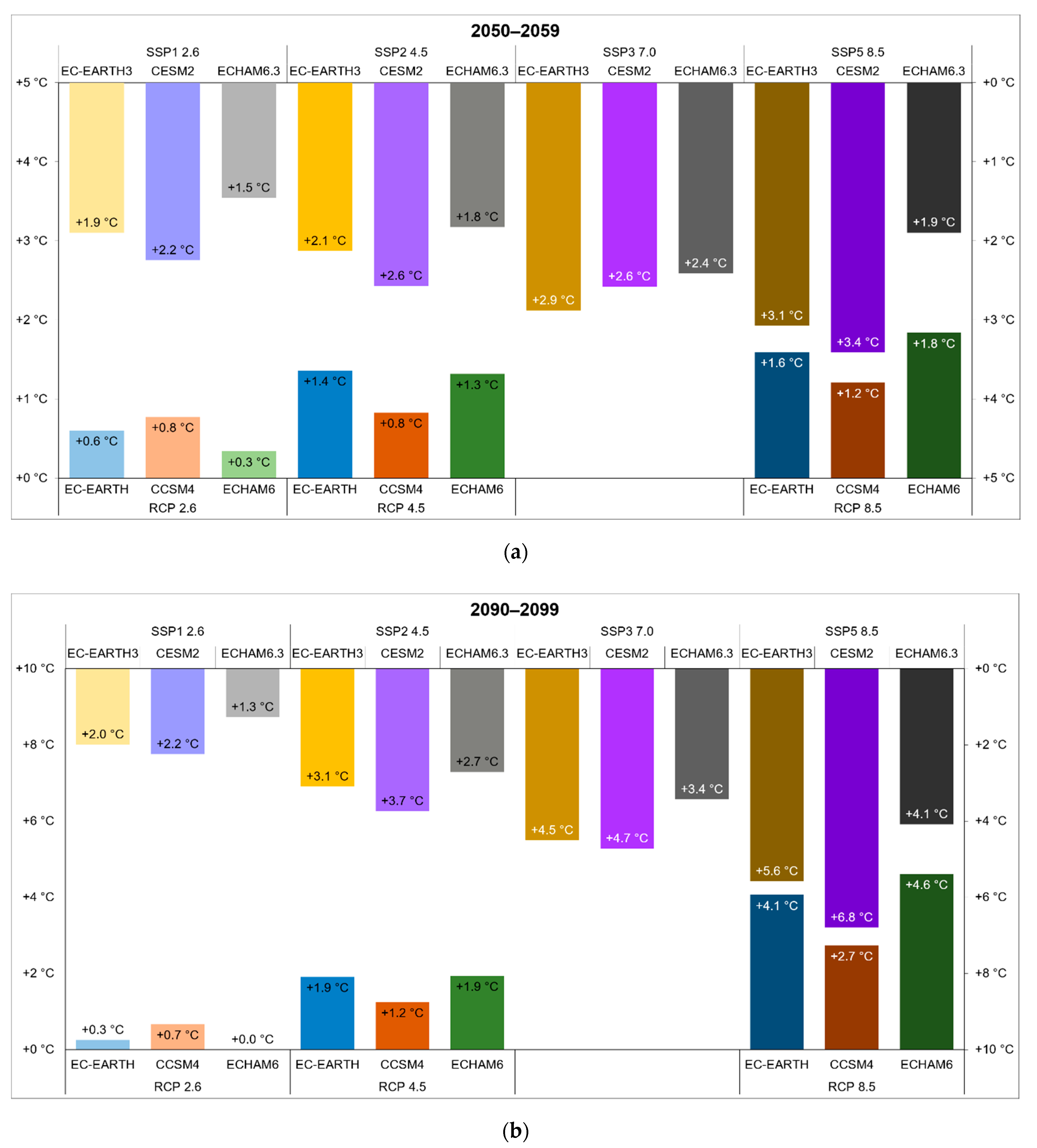
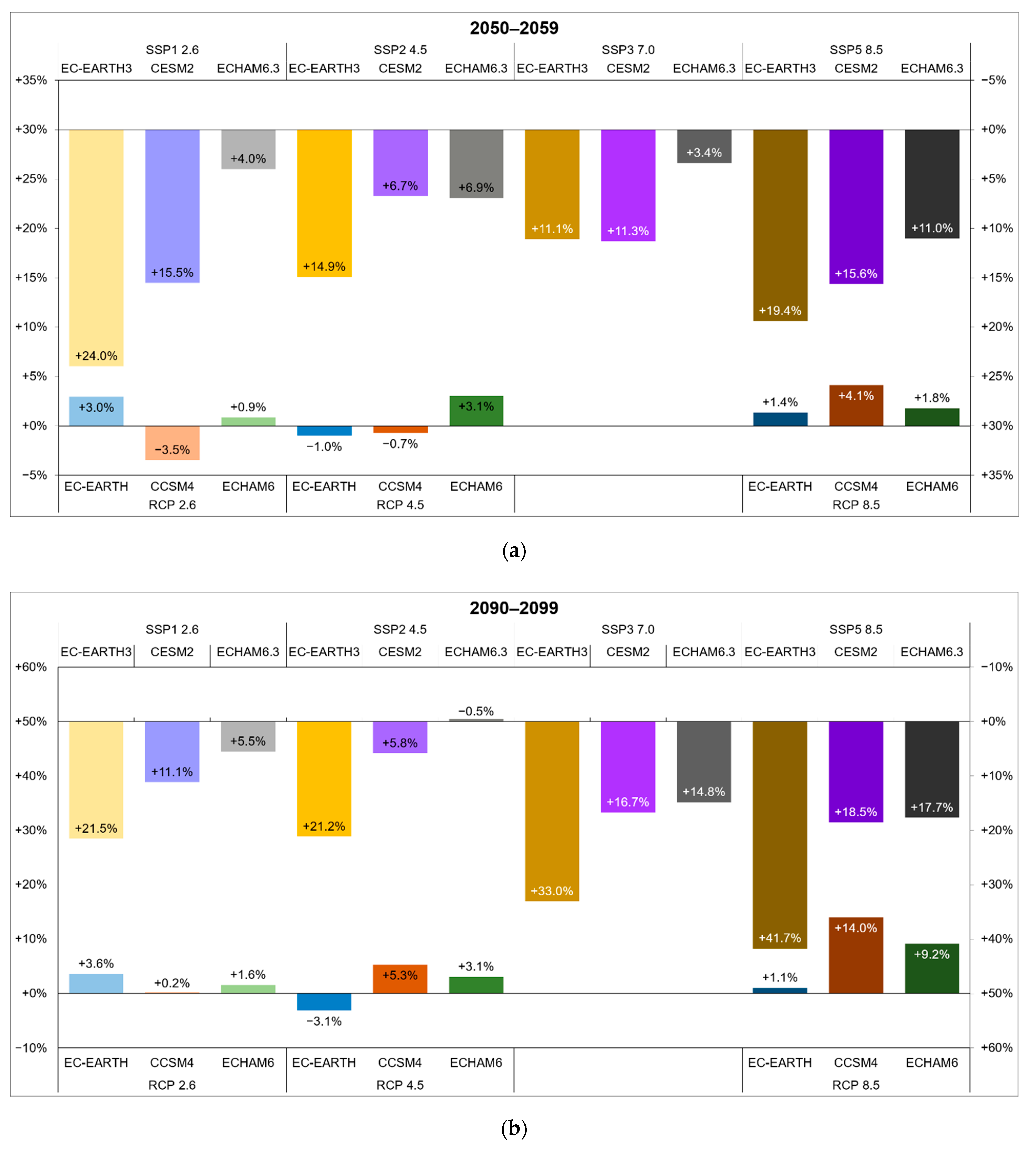
Here, we report (Figure 6 and Figure 7) changes in climatology of the area under IPCC scenarios (vs. the benchmark of CR period), in terms of mean behavior of climate in Ethiopia. We consider two reference decades, 2050–2059 (P1, Mid Century) and 2090–2099 (P2, End of Century). All projections show increased temperature (Figure 5), both under RCPs and SSPs, and larger increases at the End of Century (unless some scenarios for RCP2.6, SSP1 2.6). RCP8.5 and SSP5 8.5 show the greatest temperature increase at the end of century, as expected. Precipitation projections (Figure 7) are more sensitive to model setup. Mid Century decade P1 in CMIP5 models show increases and decreases of mean precipitation, while CMIP6 shows increased precipitation, except for MIP-ESM (ECHAM 6.3) model. In the End of Century P2 decade, except for MIP-ESM, on average precipitation would increase, possibly due to proximity to the equatorial zone, with more available energy for evaporation, and eventually more precipitation.
5.5. Future Hydrology of the Area
5.5.1. Future Hydrology at GERD Dam
Changes in precipitation and temperature clearly influence stream flows at the hydropower plants. Using the Poli-Hydro model, with inputs of future temperature and precipitation, we could provide scenarios of hydrological regimes for the P1/P2 decades (Figure 8). The CMIP5 scenarios display oscillations in both periods, while CMIP6 projections provide different results, with mostly increasing discharges.
5.5.2. Future Hydrology at GIBE III Dam
CMIP5 projections at GIBE III (Figure 8) provide again oscillating results, under different models in both P1 and P2. The results from EC-EARTH are those with larger at the end of century. CCSM4 displays the largest increase in both decades. Most recent projections (CMIP6) provide larger increases in P2 than in P1, with CESM2 and EC-EARTH3, in certain scenarios, reaching until +100% or more.
5.6. Future Hydropower Production
We report here potential changes of hydropower production, under two scenarios, namely, (i) S1 with no water release (hydropower only) and (ii) S2 with water release (GERD, agricultural demand, GIBE III, Turkana lake supply).
5.6.1. GERD No Release Scenario
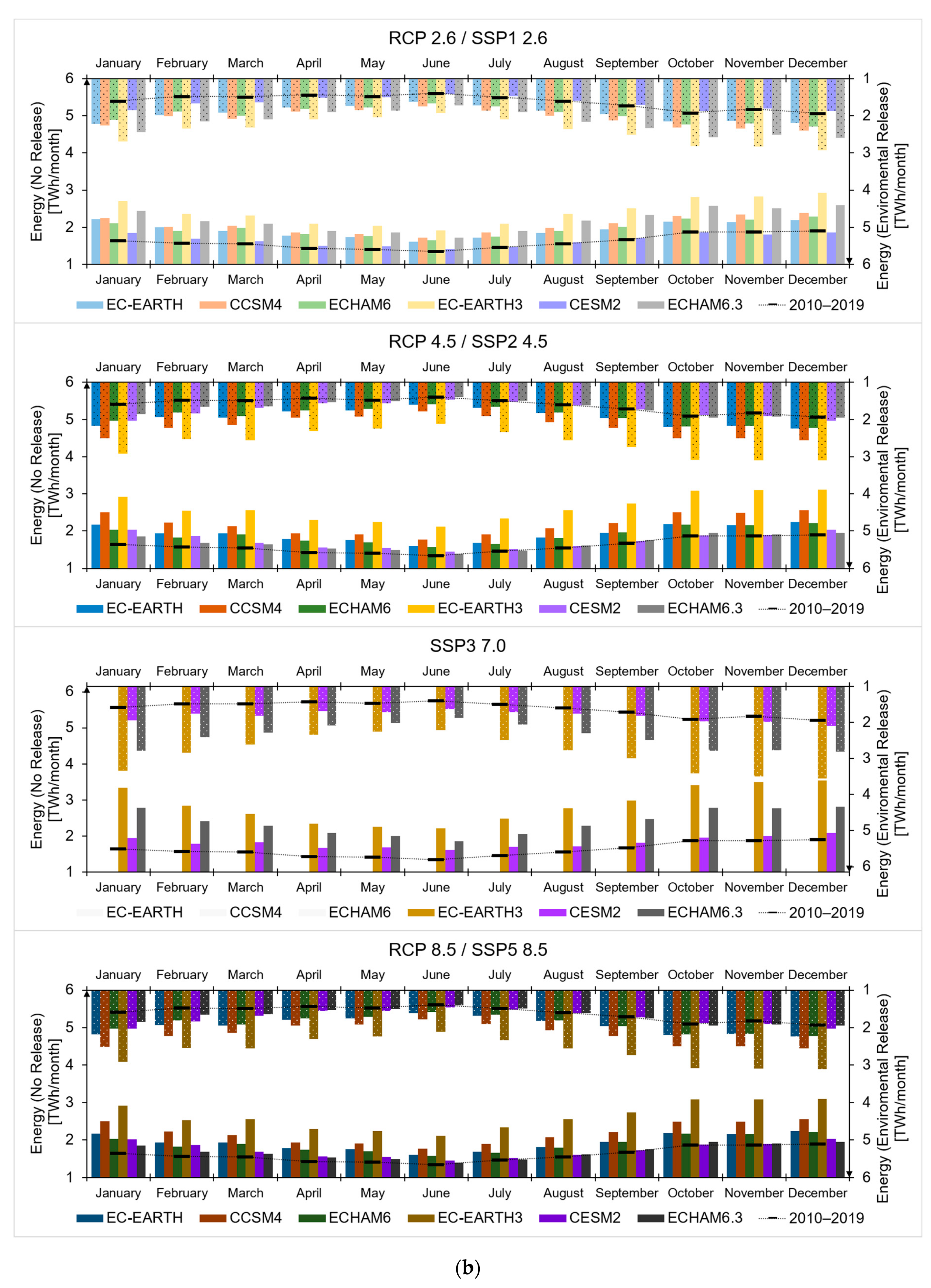
Energy production at GERD (Figure 9) increases at half century P1, with higher increase during flood periods, July–September. RCP8.5/SSP5 8.5 project largest increase yearly, and monthly, in particular, under the EC-EARTH3 model. At the end of century P2, production would be higher than in CR, but smaller than during P1. Seasonally, production would be similar to that in P1, higher at the end of summer, and lower during winter, and spring. Overall, the mean annual production for all scenarios in CMIP5 would be 23.5 and 24.6 TWh/year, respectively, during P1 and P2 (see Table 7). Accordingly, there could be a slight increase in energy production against CR (19.3 TWh/year). The CMIP6 projections depict similar behavior, with even larger production in both decades. The overall mean annual production would be 27.1 TWh/year in P1 and 25.8 TWh/year in P2. In Figure S1 of the Supplementary Material, we report changes of (monthly) pool volume of the GERD reservoir. One sees a general increase under the different scenarios, in particular, for those with a major increase of flows. In addition, this increase is more noticeable in fall and winter, when the reservoir reaches the maximum volume. This also leads to an increase in the use of the reservoir volume, reaching a fluctuation of 55–60% of the total active volume with a maximum of 88%.
5.6.2. GERD Environmental Release Scenario
Due to the large reservoir’s size, no noticeable difference of production was seen when considering the release scenario S2 in GERD, as reported. According to our simulations, this would also happen in the future, and the projected energy production in this case would be, in practice, the same as in the S1 scenario, as shown in Figure 9. As for the energy production, no change in pool volume can be appreciated in the Table S1/S2 comparison, as seen in Figure S1 of the Supplementary Material.
5.6.3. GIBE III No Release Scenario
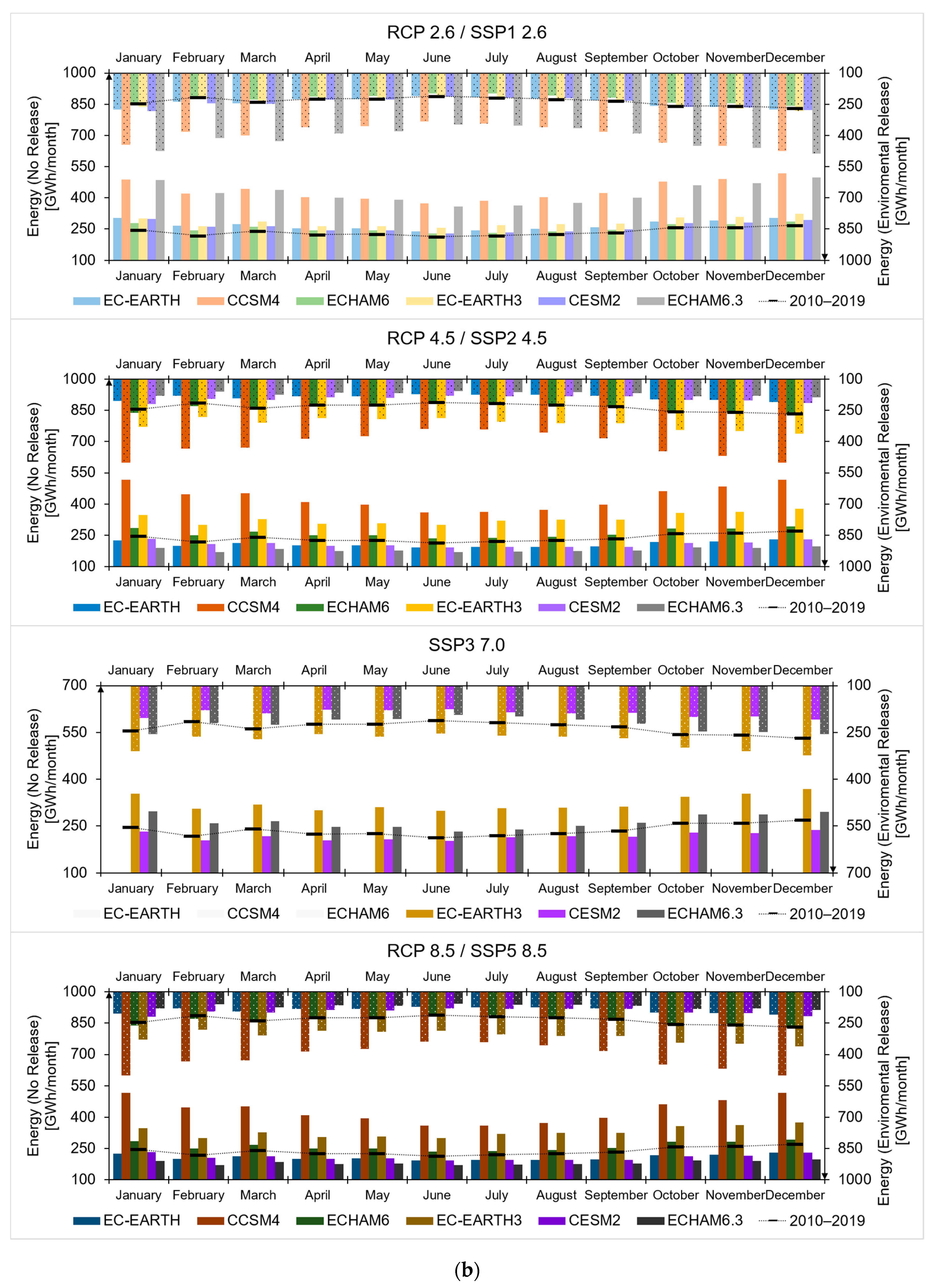
Figure 10 provides the projected monthly production at Mid and End of Century for GIBE III under No Release S1 management scenario. Therein, one has on average a lower energy production against CR, both for CMIP5 and CMIP6. In CMIP5, the model CCSM4 always displays the largest production, while the EC-EARTH3 always shows the smallest. Seasonally, the production increases between May and August, and then it decreases at the end of the year. The overall mean annual production would be 3.7 and 4.1 TWh/year respectively, in P1 and P2, much larger than now (2.8 TWh/year). The new projections from CMIP6 have similar behavior, with greatest energy production during the flood season. The overall mean annual production would be 3.0 and 3.4 TWh/year, respectively, in P1 and P2, with a slight increase in energy production at the end of century. In Figure S2 in the Supplementary Material, we report the changes in reservoir’s volume for the S1 scenario. A change between the different scenarios and decades, with respect to the CR, is not evident here.
5.6.4. Gibe III Environmental Release Scenario
Under CMIP5 scenarios (Figure 10), in the Environmental Release Scenario, energy production at GIBE III increases with respect to the CR period, slightly during winter and spring and largely in summer during the flood season. This happens for both reference decades. The overall annual production would be 3.5 and 3.4 TWh/year, respectively, in P1 and P2, slightly larger than now (2.8 TWh/year, see Table 8).
The new projections of CMIP6 (Figure 10) give similar results, with similar production patterns, and production mostly increasing against CR. However, the mean annual energy production would be smaller than under the CMIP5 scenarios, namely, 2.8 and 2.9 TWh/year (however, larger than CR). Under the Environmental Release Scenario S2, the pool volume dynamics (Figure S2, Table S2, Supplementary Material) is different with respect to S1 scenario, and a clear decrease against the control run is visible both in P1 and P2 under most scenarios (SSP2,3,5). The change is most evident for the CMIP6 scenario, particularly at the end of century P2. The fluctuation inside the reservoir is also greater, reaching also value of 55%, larger than under the CR scenario.
6. Discussion
6.1. Hydropower Production under Climate Change
Assessment of future expected energy production requires proper hydrological knowledge, complex given the complex topography of the catchments of interest, and sparseness of the data base in our knowledge. Accurate hydrological modeling is necessary, to quantify the nexus between climate, water fluxes, and hydropower production. Here, use of the Poli-Hydro model was well suited in this respect [25,26,27,28,52]. In addition, we were able to use the Poli-Power model, to depict optimal reservoir’s operation under present, and future hydro-climatological conditions. We considered explicitly the variability of price/demand against climate, and economic growth, a complex dynamic often neglected in recent studies covering present, and future hydropower potential [26].
The scenarios investigated in [26] suggest that possible future climatic trends will not substantially impact hydropower production on a national level (therein in Italy, a Mediterranean country). Yet, at the local level, individual hydropower plants may be subject to precipitation variability (plus/minus) coming from climate change that could lead to larger/smaller hydropower production losses than on average nation-wide.
We explored here potential operation of GERD and GIBE III reservoirs under two possible operation scenarios, one including explicit consideration of the water needs of Egypt and Sudan downstream GERD, and the environmental volumes needed to replace evaporation from Turkana lake in (Ethiopia and) Kenya. Operation under such scenarios may dampen water-based tensions between Ethiopia, and its downstream neighbors.
For GERD reservoir, we showed that under the S1/S2 scenarios with optimal reservoir’s operation, the production and revenues for Ethiopia’s government would be the same in practice. This happens because the hydropower plant properties are so peculiar that the influence of a minimum value for turbine water (i.e., environmental flows under option S2, still used for hydropower) seems negligible. Optimizing the revenues, energy production could be different in time, and yet revenues for the two scenarios are the same, so no large economic loss would be seen. Apparently therefore, the GERD dam could be managed so as to avoid tensions between states. Eventually, we discovered that energy production could increase at half century, with only a slight decrease at the end (and yet higher than now).
Our assessment concerning (optimal) duration of the filling time, seemingly indicates a lowest loss in energy production, and a smallest penalization of the downstream flows (especially interesting in the S2 scenario, with fair flow release), for a 4–5 years period, consistently with recent findings (e.g., [56]).
At GIBE III, we demonstrated that under the environmental release scenario (downstream flow to Turkana), one could produce slightly less energy than under the sole hydropower release. In addition, here, energy production could increase at half century, with a slight decrease at the end of century, still higher than now. Accordingly, one may guess that, whenever such difference would be significant, in practice under S1, a slightly more rewarding use of water would be obtained (i.e., with −8% discharge used and −6% revenues). Such circumstance would indicate a (slight) loss of economic efficiency when environmental release (i.e., for Turkana lake) is considered. CMIP6 projections are slightly different from CMIP5 ones, and especially changes of precipitation are uncertain, which is widely known, and exploitation of more scenarios provides an array of possible energy pathways.
A change of the control run period may clearly provide different results in terms of expected variation in absolute terms, but the relative trend in future projections remains similar. Eventually, one could state that energy production may likely change during the century, with likely increase in the 2050s and subsequent slight decrease (but still larger than now) in the 2090s.
To better assess the dependence of energy production against weather patterns, we here explored the relationship between hydropower oscillations and the corresponding climate variables. We pursued a visual correspondence analysis between percentage variation (vs CR 2010–2019) of energy production ΔE, and of precipitation ΔP, likely to be mostly affecting hydropower dynamics. In Figure 11, we provide a chart displaying mean ΔE against ΔP, for Mid Century and End of Century, in our 21 scenarios for both dams. For reference, we report changes of ΔE/ΔP for the other decades during 2020–2099 (126 dots for each scenario S1/S2).
Concerning the GERD dam, one clearly sees a visual correspondence between the two variables ΔE/ΔP. Namely, the increase in precipitation leads to a significant increase in energy (regression coefficient of 2.05 and R2 = 0.88 for No Release scenario S1 and regression coefficient of 2.04 and R2 = 0.89 for Release scenario S2). Notice as reported that no large difference is seen in practice between the S1/S2 scenarios.
In the case of GIBE III, albeit generally a change of ΔP results into a synchronous change of ΔE, the relationship is weaker. This may derive from the fact that production here is limited more by the capacity of the reservoir and by monthly and seasonal variations, than by the annual variation of the (rainfall) input. Indeed, in some scenarios, due to the temporal combination of precipitation, the reservoir volume limits are reached and fluctuations are therefore restricted, limiting the production of energy only in this particular combination.
6.2. Limitations and Outlooks
Our study aimed to produce credible scenarios of the future expected hydrological dynamics and of hydropower production in GERD and GIBE III power plants. Our hydrological model depicts reasonably well the hydrological processes in the area. The general lack (or sparseness) of data, and the introduction of lapse rates of precipitation, and temperature with altitude might have implied approximations, possibly adding noise.
The model performs quite well, even in complex terrains, as demonstrated by several former papers, provided some deal of information is available. The calibration parameters of Poli-Hydro are ground permeability and lag times, to be tuned against flow data. Ground permeability mostly affects water volumes, which were reasonably well tuned against the available hydrological data. Slight variations as tested during a preliminary sensitivity analysis, would not affect largely the results (and clearly, runoff water volumes would depend largely upon the precipitation inputs).
Lag times would modify slightly timing of flows (see [52]), but again a preliminary sensitivity analysis demonstrated small changes in model performance. Most importantly, given the large size of the reservoirs, and the smoothing effects of water storage thereby, noise in discharge assessment did not result into visible changes in reservoir management, and hydropower production. In this sense, the model shows some robustness.
Here, the purpose was not to develop a (very) accurate hydrological model, but more to simulate potential for hydropower production, and possible changes in the future. Considering the size of the reservoirs as suggested above, noise in (daily) discharge assessment should not result into large error in reservoir management overall, and as well such noise should not disturb largely assessment of future production.
All GCMs, RCPs, and SSPs give future projections, so clearly embedding uncertainty and approximations, affecting the Poli-Hydro and Poli-Power models. Investigations of a larger array of possible scenarios (i.e., more GCMs/RCPs/SSPs) may add more insight.
Regarding RCPs and SSPs, in principle all of them can be taken as equally likely until the end of the century, so they represent equally possible evolutions of climate and of hydropower systems in cascade. However, recent findings [57,58] indicates that recent global climate resembles more closely the scenarios as projected under RCP8.5, and possibly such scenarios (and SPP8.5) may be seen more likely for design.
Among others, Adera et al. [59] studied the Tekeze hydropower plant located in the Tekeze river basin in the northern part of Ethiopia, another Nile river tributary. They used a combination of different regional climate model, and they showed potential increase in precipitation that my lead to an increase in energy production. Abera et al. [60] in the same basin found also a similar pattern in precipitation and temperature increase, with consequent increase of discharge. They find a potential increase of the water volume stored in the reservoir, leading to an increase in production, similarly to what we found here for the GERD reservoir.
Further work may be devoted to obtaining data (whenever available) from hydrometric stations of the Ministry of Water Irrigation and Energy, owning, and operating streamflow stations in Ethiopia. Use of longer, more recent flow series may improve hydrological modeling. Finally, having access to energy production data from the plants may significantly improve the accuracy of energy production modeling, and projecting.
7. Conclusions
In the present study, we found that in the 21st century under climate change as expected, Ethiopia may count upon constant (if not increased) hydropower production from its largest dams GERD and GIBE III (and from GIBE I and GIBE II, however, small). Given the complexity of the nexus between climate, water flows, and hydropower production, accurate modelling is necessary to quantify present and future dynamics thereby. The Poli-Hydro, and Poli-Power models are suitable tools for the purpose of assessing optimal reservoir’s operation under present and future hydrological conditions, also considering explicitly the changes in economy, population growth, the presence of constrains, and agreements between nations.
Our results surely provide ground for discussion, for the assessment of future hydrology of the area of interest, and generally of Ethiopia, and subsequent impact upon operation, and production in the large dams GERD and GIBE III, fundamental for the future of Ethiopia energy-wise.
The projected patterns will have to be monitored, and updated on track. However, they are usable already now for an assessment of the potential for future evolutions, brainstorming of adaptation, and even planning of shared water management with bordering countries.
Our tool, exportable to other similar catchments/reservoirs, may be of use for scientists, policy makers, hydropower companies, and in general, for investigation of energy strategies for the future, in Ethiopia and elsewhere.
Supplementary Materials
The following are available online at https://www.mdpi.com/2073-4441/13/5/716/s1, Figure S1: GERD. Average estimated monthly pool volume. (a) Mid Century P1. (b) End of Century P2, Figure S2: GIBE III. Average estimated monthly pool volume. (a) Mid Century P1. (b) End of Century P2; Table S1: GERD. Average estimated yearly pool volume; Table S2. GIBE III. Average estimated yearly pool volume.
Author Contributions
Conceptualization, D.B. and A.B.; methodology, S.T. and G.M.B.; software, G.M.B. and S.T.; validation, S.T.; formal analysis, S.T.; investigation, S.T.; resources, D.B.; data curation, S.T. and G.M.B.; writing—original draft preparation, S.T. and G.M.B.; writing—review and editing, D.B. and A.B.; visualization, G.M.B. and S.T.; supervision, D.B. and A.B.; project administration, D.B.; funding acquisition, D.B. All authors have read and agreed to the published version of the manuscript.
Funding
This research received no external funding.
Data Availability Statement
Data available upon request. The data presented in this study are available on request from the corresponding author.
Acknowledgments
This work reports results in fulfilment of Eng. Stefano Tomiet MS Thesis. The authors kindly acknowledge support from Climate-Lab, the Interdepartmental Laboratory on Global Climate Change at Politecnico di Milano. https://www.climatelab.polimi.it/ (accessed on 5 March 2021). Four anonymous reviewers are kindly acknowledged for helping to improve the quality of the manuscript.
Conflicts of Interest
The authors declare no conflict of interest that they are aware of.
Abbreviations
| GERD | Grand Ethiopian Renaissance Dam |
| CMIP5 | Coupled Model Intercomparison Project 5 |
| CMIP6 | Coupled Model Intercomparison Project 6 |
| IPCC | Intergovernmental Panel on Climate Change |
| NOAA | National Oceanic and Atmospheric Administration |
| DEM | Digital Elevation Model |
| CN | Curve Number |
| CGLS | Copernicus Global Land Service |
| NSE | Nash-Sutcliffe Efficiency |
| GCM | Global Circulation Model |
| EC-Earth | European Consortium Earth system model |
| CCSM4 | Community System Model |
| CESM2 | Community Earth System Model |
| MPI-ESM | European Center Hamburg Model |
| RCP | Representative Concentration Pathways |
| SSP | Shared Socio-economic Pathways |
| CR | Control Run 2010–2019 |
| P1 | Mid Century 2050–2059 |
| P2 | End of Century 2090–2099 |
| S1 | No Release Scenario |
| S2 | Environmental Release Scenario |
References
- Yüksel, I. Hydropower for sustainable water and energy development. Renew. Sustain. Energy Rev. 2010, 14, 462–469. [Google Scholar] [CrossRef]
- FDRE. Federal Democratic Republic of Ethiopia Ministry of Water and Energy. Scaling-Up Renewable Energy Program Ethiopia Investment Plan (Draft Final). January 2012. [Google Scholar]
- Mulat, A.G.; Moges, S.A. Assessment of the Impact of the Grand Ethiopian Renaissance Dam on the Performance of the High Aswan Dam. J. Water Resour. Prot. 2014, 6, 583–598. [Google Scholar] [CrossRef] [Green Version]
- Ministry of Mines and Energy Ethiopian Electric Light and Power Authority. Gilgel Gibe Hydroelectric Project, July 1997.
- Conway, D. A water balance model of the Upper Blue Nile in Ethiopia. Hydrol. Sci. J. 1997, 42, 265–286. [Google Scholar] [CrossRef] [Green Version]
- Conway, D. The climate and hydrology of the Upper Blue Nile river. Geogr. J. 2000, 166, 49–62. [Google Scholar] [CrossRef] [Green Version]
- Elganainy, M.A.; Eldwer, A.E. Stochastic forecasting models of the monthly stream flow for the Blue Nile at Eldiem station. Water Resour. 2018, 45, 326–337. [Google Scholar] [CrossRef]
- Melesse, A.M.; Abtew, W.; Setegn, S.G.; Dessalegne, T. Hydrological variability and climate of the Upper Blue Nile River Basin. In Nile River Basin: Hydrology, Climate and Water Use; Springer: Dordrecht, The Netherlands, 2011; pp. 3–37. [Google Scholar]
- Gleick, P.H. The vulnerability of runoff in the Nile basin to climatic changes. Environ. Prof. 1991, 13, 66–73. [Google Scholar]
- Conway, D.; Hulme, M. Recent fluctuations in precipitation and runoff over the Nile subbasins and their impact on Main Nile discharge. Clim. Chang. 1993, 25, 127–151. [Google Scholar] [CrossRef]
- Conway, D.; Hulme, M. The impacts of climate variability and future climate change in the Nile basin on water resources in Egypt. Water Resour. Dev. 1996, 12, 277–296. [Google Scholar] [CrossRef]
- Strzepek, K.M.; Yates, D.N. Economic and social adaptation to climate change impacts on water resources: A case study of Egypt. Water Resour. Dev. 1996, 12, 229–244. [Google Scholar] [CrossRef]
- Sene, K.J.; Tate, E.L.; Farquharson, F.A.K. Sensitivity studies of the impacts of climate change on White Nile flows. Clim. Chang. 2001, 50, 177–208. [Google Scholar] [CrossRef]
- Conway, D. From headwater tributaries to international river: Observing and adapting to climate variability and change in the Nile Basin. Glob. Environ. Chang. 2005, 15, 99–114. [Google Scholar] [CrossRef]
- Bank World. Country Water Resources Assistance Strategy Ethiopia: Managing Water Resources to Maximize Economic Growth. Washington. 2006. Available online: http://documents1.worldbank.org/curated/en/947671468030840247/pdf/360000REVISED01final1text1and1cover.pdf (accessed on 5 March 2021).
- Worqlul, A.W.; Dile, Y.T.; Ayana, E.K.; Jeong, J.; Adem, A.A.; Gerik, T. Impact of Climate Change on Streamflow Hydrology in Headwater Catchments of the Upper Blue Nile Basin, Ethiopia. Water 2018, 10, 120. [Google Scholar] [CrossRef] [Green Version]
- Intergovernmental Panel on Climate Change (IPCC). Managing the Risks of Extreme Events and Disasters to Advance Climate Change Adaptation: Special Report of the Intergovernmental Panel on Climate Change 2012; Cambridge University Press: New York, NY, USA, 2012. [Google Scholar]
- Parry, M.L.; Canziani, O.; Palutikof, J.P.; van der Linden, P.J.; Hanson, C.E. Contribution of Working Group II to the Fourth Assessment Report of the Intergovernmental Panel on Climate Change; Climate Change; Cambridge University Press: Cambridge, UK; New York, NY, USA, 2007. [Google Scholar]
- Worqlul, A.W.; Jeong, J.; Dile, Y.T.; Osorio, J.; Schmitter, P.; Gerik, T.; Srinivasan, R.; Clarke, N. Assessing potential land suitable for surface irrigation using groundwater in Ethiopia. Appl. Geogr. 2017, 85, 1–13. [Google Scholar] [CrossRef]
- Akbari-Alashti, H.; Soncini, A.; Dinpashoh, Y.; Fakheri-Fard, A.; Talatahari, S.; Bocchiola, D. Operation of two major reservoirs of Iran under IPCC scenarios during the XXI century. Hydrol. Process. 2018, 32, 3254–3271. [Google Scholar]
- IPCC. Summary for Policymakers. In Climate Change 2013: The Physical Science Basis. Contribution of Working Group I to the Fifth Assessment Report of the Intergovernmental Panel on Climate Change; Stocker, T.F., Qin, D., Plattner, G.-K., Tignor, M., Allen, S.K., Boschung, J., Nauels, A., Xia, Y., Bex, V., Midgley, P.M., Eds.; Cambridge University Press: Cambridge, UK; New York, NY, USA, 2013; Available online: http://www.climatechange2013.org/images/report/WG1AR5_Frontmatter_FINAL.pdf (accessed on 31 July 2019).
- Li, J.; Wang, Z.; Wu, X.; Ming, B.; Chen, L.; Chen, X. Evident response of future hydropower generation to climate change. J. Hydrol. 2020, 590, 125385. [Google Scholar] [CrossRef]
- Tarroja, B.; Forrest, K.; Chiang, F.; AghaKouchak, A.; Samuelsen, S. Implications of hydropower variability from climate change for a future, highly-renewable electric grid in California. Appl. Energy 2019, 237, 353–366. [Google Scholar] [CrossRef]
- Menne, M.J.; Durre, I.; Vose, R.S.; Gleason, B.E.; Houston, T.G. An overview of the Global Historical Climatology Network-Daily Database. J. Atmos. Ocean. Technol. 2012, 29, 897–910. [Google Scholar] [CrossRef]
- Bocchiola, D.; Soncini, A.; Senese, A.; Diolaiuti, G. Modelling hydrological components of the Rio Maipo of Chile, and their prospective evolution under climate change. Climate 2018, 6, 57. [Google Scholar] [CrossRef] [Green Version]
- Bombelli, G.M.; Soncini, A.; Bianchi, A.; Bocchiola, D. Potentially modified hydropower production under climate change in the Italian Alps. Hydrol. Process. 2019, 33, 2355–2372. [Google Scholar] [CrossRef]
- Bocchiola, D.; Soncini, A. Water Resources Modeling and Prospective Evaluation in the Indus River Under Present and Prospective Climate Change. In Indus River Basin; Elsevier: Amsterdam, The Netherlands, 2019; pp. 17–56. [Google Scholar]
- Stucchi, L.; Bombelli, G.M.; Bianchi, A.; Bocchiola, D. Hydropower from the Alpine Cryosphere in the Era of Climate Change: The Case of the Sabbione Storage Plant in Italy. Water 2019, 11, 1599. [Google Scholar] [CrossRef] [Green Version]
- International Panel of Experts. International Panel of Experts on Grand Ethiopian Renaissance Dam Project. 2013. Available online: https://www.scidev.net/wp-content/uploads/site_assets/docs/international_panel_of_experts_for_ethiopian_renaissance_dam-_final_report.pdf (accessed on 5 March 2021).
- Pietrangeli, G.; Alberti, D. Design of Grand Ethiopian Renaissance RCC Main Dam. 2016. Available online: https://www.pietrangeli.com/img/publish/634-DESIGN-OF-GRAND-ETHIOPIAN-RENAISSANCE,-RCC-MAIN-DAM-H-175-m-Pietrangeli-Bezzi,-Rossini-Masciotta,-DAlberti-2017.pdf (accessed on 5 March 2021).
- Parisella, P.; Cozzolino, G.; Levi, G.; Tere, G.; Bregato, B.; Cassese, F.; Sacco, P. Ex-Post valuation of the Italian Development Cooperation Initiative in Ethiopia Named “Gilgel Gibe II Hydroelectric Project” Commissioned by MINISTRY OF FOREIGN AFFAIRS General Directorate for Development Cooperation FINAL REPORT Ex-Post Evaluation. 2012. Available online: https://dafne.ethz.ch/wp-content/uploads/2020/10/DAFNE_D21.pdf (accessed on 5 March 2021).
- Cagiano, A.; De Azevedo, A.; Masciotta, A.; Pianigiani, F.; Pietrangeli, A. Design and Hydraulic Model of the Gibe III Dam Spillway. 2015. Available online: https://www.pietrangeli.com/img/publish/135-DESIGN-AND-HYDRAULIC-MODEL-OF-GIBE-III-DAM-SPILLWAY,-Cagiano-A-,-Masciotta-A-,-Pianigiani-F-,-Pietrangeli-A-,-2015.pdf (accessed on 5 March 2021).
- Asnake, A.; Cagiano, A.; Ferraro, B.; Zoppis, E.; Studio Pietrangeli. Managing unprecedented RCC challenges at Gibe III dam. Ethiopia 2015, 2015, 58–63. [Google Scholar]
- Asnake, A. Environmental and Social Impact Assessment Executive Summary—GIBE III Hydrolectric Power Project (P-ET-FAB-005); African Development Bank: Tunis, Tunisia, 2015; Available online: https://www.afdb.org/fileadmin/uploads/afdb/Documents/Project-and-Operations/GIIBE%20III%20RAP%20Executive%20Summary%20-%20EBNJK%20%2006-08-08.pdf (accessed on 5 March 2021).
- NASA/METI/AIST/Japan Spacesystems; U.S./Japan ASTER Science Team. ASTER Global Digital Elevation Model V003 [Data set]. NASA EOSDIS Land Processes DAAC. 2019. Available online: https://doi.org/10.5067/ASTER/ASTGTM.003 (accessed on 22 July 2020).
- GRDC (Global Runoff Data Centre). Dataset Daily River Discharge Time Series from the Global Runoff Data Centre, D—56068 Koblenz, Germany. 2007. Available online: http://grdc.bafg.de (accessed on 1 April 2020).
- Buchhorn, M.; Smets, B.; Bertels, L.; Lesiv, M.; Tsendbazar, N.E.; Herold, M.; Fritz, S. Copernicus Global Land Service: Land Cover 100 m: Epoch 2015: Globe. Dataset Glob. Compon. Copernic. Land Monit. Serv. 2019. [Google Scholar] [CrossRef]
- AQUASTAT; FAO. FAO’s Information System on Water and Agriculture; Food and Agriculture Organization of the United Nations (FAO): Rome, Italy, 2011. [Google Scholar]
- Avery, S. Hydrological Impacts of Ethiopia’s Omo Basin on Kenya’s Lake Turkana Water Levels and Fisheries—Final Report; African Development Bank: Tunis, Tunisia, 2011; Available online: https://www.afdb.org/en/documents/document/ethiopia-hydrological-impacts-of-ethiopias-omo-basin-on-kenyas-lake-turkana-water-levels-and-fisheries-final-report-24642 (accessed on 5 March 2021).
- Taylor, K.E.; Stouffer, R.J.; Meehl, G.A. An overview of CMIP5 and the experiment design. Bull. Am. Meteorol. Soc. 2012, 93, 485–498. [Google Scholar] [CrossRef] [Green Version]
- O’Neill, B.C.; Tebaldi, C.; van Vuuren, D.P.; Eyring, V.; Friedlingstein, P.; Hurtt, G.; Knutti, R.; Kriegler, E.; Lamarque, J.-F.; Lowe, J.; et al. The Scenario Model Intercomparison Project (ScenarioMIP) for CMIP6. Geosci. Model Dev. 2016, 9, 3461–3482. [Google Scholar] [CrossRef] [Green Version]
- Hazeleger, W.; Severijns, C.; Semmler, T.; Stefanescu, S.; Yang, S.; Wang, X.; Bougeault, P. EC-Earth: A seamless earth-system prediction approach in action. Bull. Am. Meteorol. Soc. 2010, 91, 1357–1364. [Google Scholar] [CrossRef] [Green Version]
- EC-Earth Consortium (EC-Earth). EC-Earth-Consortium EC-Earth3 Model Output Prepared for CMIP6 ScenarioMIP; Earth System Grid Federation, 2019. Available online: https://esgf.llnl.gov/ (accessed on 5 March 2021).
- Gent, P.R.; Danabasoglu, G.; Donner, L.J.; Holland, M.M.; Hunke, E.C.; Jayne, S.R. The community climate system model version 4. J. Clim. 2011, 24, 4973–4991. [Google Scholar] [CrossRef]
- Danabasoglu, G. NCAR CESM2 Model Output Prepared for CMIP6 ScenarioMIP; Earth System Grid Federation, 2019. Available online: https://esgf.llnl.gov/ (accessed on 5 March 2021).
- Stevens, B.; Giorgetta, M.; Esch, M.; Mauritsen, T.; Crueger, T.; Rast, S.; Brokopf, R. Atmospheric component of the MPI-M earth system model: ECHAM6. J. Adv. Model. Earth Syst. 2013, 5, 146–172. [Google Scholar] [CrossRef]
- Schupfner, M.; Wieners, K.; Wachsmann, F.; Steger, C.; Bittner, M.; Jungclaus, J.; Früh, B.; Pankatz, K.; Giorgetta, M.; Reick, C.; et al. DKRZ MPI-ESM1.2-HR Model Output Prepared for CMIP6 ScenarioMIP; Earth System Grid, 2019. Available online: https://esgf.llnl.gov/ (accessed on 5 March 2021).
- Groppelli, B.; Soncini, A.; Bocchiola, D.; Rosso, R. Evaluation of future hydrological cycle under climate change scenarios in a mesoscale alpine watershed of Italy. Nat. Hazards Earth Syst. Sci. 2011, 11, 1769–1785. [Google Scholar] [CrossRef] [Green Version]
- Groppelli, B.; Bocchiola, D.; Rosso, R. Spatial downscaling of precipitation from GCMs for climate change projections using random cascades: A case study in Italy. Water Resour. Res. 2011, 47, W03519. [Google Scholar] [CrossRef]
- Moss, R.H.; Edmonds, J.A.; Hibbard, K.A.; Manning, M.R.; Rose, S.K.; Van Vuuren, D.P. The next generation of scenarios for climate change research and assessment. Nature 2010, 463, 747–756. [Google Scholar] [CrossRef]
- Riahi, K.; Van Vuuren, D.P.; Kriegler, E.; Edmonds, J.; Neill, B.C.O.; Fujimori, S. The Shared Socioeconomic Pathways and their energy, land use, and greenhouse gas emissions implications: An overview. Glob. Environ. Chang. 2017, 42, 153–168. [Google Scholar] [CrossRef] [Green Version]
- Soncini, A.; Bocchiola, D.; Azzoni, R.S.; Diolaiuti, G. A methodology for monitoring and modeling of high altitude Alpine catchments. Prog. Phys. Geogr. 2017, 41, 393–420. [Google Scholar] [CrossRef]
- Rosso, R. Nash Model Relation to Horton Order Ratios. Water Resour. Res. 1984, 20, 914–920. [Google Scholar] [CrossRef]
- Hargreaves, G.H. The estimation of potential and crop evapotranspiration. Am. Soc. Agric. Eng. Trans. 1974, 17, 701–704. [Google Scholar] [CrossRef]
- Bombelli, G.M.; Soncini, A.; Bianchi, A.; Bocchiola, D. Prospective climate change impacts upon energy prices in the 21st century: A case study in Italy. Climate 2019, 7, 121. [Google Scholar] [CrossRef] [Green Version]
- Elsanabary, M.H.; Ahmed, A.T. Impacts of Constructing the Grand Ethiopian Renaissance Dam on the Nile River. In Grand Ethiopian Renaissance Dam Versus Aswan High Dam. The Handbook of Environmental Chemistry, 79; Negm, A., Abdel-Fattah, S., Eds.; Springer: Cham, Switzerland, 2018. [Google Scholar] [CrossRef]
- Fuss, S.; Canadell, J.G.; Peters, G.P.; Tavoni, M.; Andrew, R.M.; Ciais, P.; Le Quéré, C. Betting on negative emissions. Nat. Clim. Chang. 2014, 4, 850–853. [Google Scholar] [CrossRef]
- Zwaan, B.; Boccalon, A.; Dalla Longa, F. Prospects for hydropower in Ethiopia: An energy-water nexus analysis. Energy Strategy Rev. 2017, 19. [Google Scholar] [CrossRef]
- Adera, A.G.; Alfredsen, K.T. Climate change and hydrological analysis of Tekeze river basin Ethiopia: Implication for potential hydropower production. J. Water Clim. Chang. 2020, 11, 744–759. [Google Scholar] [CrossRef] [Green Version]
- Abera, F.F.; Asfaw, D.H.; Engida, A.N.; Melesse, A.M. Optimal Operation of Hydropower Reservoirs under Climate Change: The Case of Tekeze Reservoir, Eastern Nile. Water 2018, 10, 273. [Google Scholar] [CrossRef] [Green Version]
Figure 1.
Regions of study in Ethiopia. DEM (Digital Elevation Model) of Blue Nile and Omo catchments closed at dam sites. We also report the stream flow and meteorological stations used in the study.
Figure 1.
Regions of study in Ethiopia. DEM (Digital Elevation Model) of Blue Nile and Omo catchments closed at dam sites. We also report the stream flow and meteorological stations used in the study.

Figure 2.
Hypsographic curve at dam sites. (a) Grand Ethiopian Renaissance Dam (GERD) and (b) GIBE.


Figure 3.
Monthly flows during the calibration period (1965–1988), at dam sites and river discharge stations. (a) Blue Nile basin, GERD. (b) Omo basin, GIBE. We also report flow components (surface/subsurface).
Figure 3.
Monthly flows during the calibration period (1965–1988), at dam sites and river discharge stations. (a) Blue Nile basin, GERD. (b) Omo basin, GIBE. We also report flow components (surface/subsurface).


Figure 4.
Mean monthly potential hydropower productions, discharge release, and water volumes stored in the reservoir during CR (2010–2019), with No Release (S1, solid lines), and Environmental Release (S2, dotted lines). (a) GERD and (b) GIBE.
Figure 4.
Mean monthly potential hydropower productions, discharge release, and water volumes stored in the reservoir during CR (2010–2019), with No Release (S1, solid lines), and Environmental Release (S2, dotted lines). (a) GERD and (b) GIBE.


Figure 5.
MIF loss, and energy loss for the GERD dam, depending upon of different duration of the filling period, from 1 to 10 years. Simulation during 2010–2019.
Figure 5.
MIF loss, and energy loss for the GERD dam, depending upon of different duration of the filling period, from 1 to 10 years. Simulation during 2010–2019.

Figure 6.
Average yearly temperature variations. (a) Mid Century P1. (b) End of Century P2.

Figure 7.
Average yearly precipitation variations. (a) Mid Century P1. (b) End of Century P2.

Figure 8.
Yearly stream flow changes in GERD and GIBE III. (a) Mid Century P1. (b) End of Century P2.
Figure 8.
Yearly stream flow changes in GERD and GIBE III. (a) Mid Century P1. (b) End of Century P2.

Figure 9.
GERD. Average estimated monthly hydropower production. (a) Mid Century P1. (b) End of Century P2.
Figure 9.
GERD. Average estimated monthly hydropower production. (a) Mid Century P1. (b) End of Century P2.


Figure 10.
GIBE III. Average estimated monthly hydropower production. (a) Mid Century P1. (b) End of Century P2.
Figure 10.
GIBE III. Average estimated monthly hydropower production. (a) Mid Century P1. (b) End of Century P2.


Figure 11.
Energy production changes ΔE, against precipitation changes ΔP: (a) GERD and (b) GIBE III.
Figure 11.
Energy production changes ΔE, against precipitation changes ΔP: (a) GERD and (b) GIBE III.


Table 1.
Characteristics of hydropower stations and related dams.
| Dams and Power Stations | |||||||
|---|---|---|---|---|---|---|---|
| Hydropower Station | Installed Power (MW) | Max Discharge (m3/s) | N° Turbines | Type of Turbines | Dam Volume (Mm3) | Dam Operation Volume (Mm3) | Basin Area (km2) |
| GERD | 6000 | 4305 | 16 | Francis | 74,000 | 59,000 | 168,000 |
| GIBE I | 210 | 101.5 | 3 | Francis | 830 | 711 | 4040 |
| GIBE II | 420 | 101.5 | 4 | Pelton | – | – | 80 |
| GIBE III | 1870 | 950 | 10 | Francis | 14,700 | 11,750 | 32,500 |
Table 2.
Meteorological stations of National Oceanic and Atmospheric Administration (NOAA) used in the study.
Table 2.
Meteorological stations of National Oceanic and Atmospheric Administration (NOAA) used in the study.
| Meteorological Stations | |||||
|---|---|---|---|---|---|
| Station | Latitude (°) | Longitude (°) | Elevation (m a.s.l.) | Start | End |
| Addis Ababa Bole | 9.03 | 38.75 | 2354 | 13 February 1957 | 24 September 2019 |
| Arba Minch | 6.08 | 37.63 | 1290 | 13 February 1957 | 24 September 2019 |
| Awassa | 7.08 | 38.48 | 1750 | 11 July 1972 | 24 September 2019 |
| Bahar Dar | 11.60 | 37.42 | 1770 | 8 July 1961 | 31 December 1988 |
| Debre Marcos | 10.33 | 37.67 | 2515 | 1 November 1953 | 31 December 1987 |
| Gondar | 12.55 | 37.42 | 1967 | 1 June 1952 | 24 September 2019 |
| Gore | 8.15 | 35.53 | 2002 | 1 June 1952 | 24 September 2019 |
| Harar Meda | 8.73 | 38.95 | 1900 | 1 January 1951 | 31 December 1988 |
| Jimma | 7.67 | 36.83 | 1725 | 1 June 1952 | 24 September 2019 |
| Lekemte | 9.08 | 36.45 | 2080 | 1 December 1970 | 31 December 1987 |
Table 3.
Hydrological stations used in the study.
| Hydrological Stations | |||||
|---|---|---|---|---|---|
| Station | Latitude (°) | Longitude (°) | Elevation (m a.s.l.) | Start | End |
| Sudan Border | 11.23 | 34.97 | 495 | 1969 | 1975 |
| Tana Lake | 11.58 | 37.40 | 1787 | 1969 | 1975 |
| Wenz | 8.23 | 37.58 | 1089 | 1976 | 1983 |
| Wolkite | 8.25 | 37.77 | 1766 | 1978 | 1980 |
Table 4.
Calibration of Poli-Hydro model. Blue Nile. In bold, values of the calibration parameters.
| Blue Nile Basin Parameters | ||||
|---|---|---|---|---|
| Unit | Description | Value | Method | |
| fv | [%] | Vegetation cover, average | 20 | Land Cover |
| K | [mmd−1] | Saturated conductivity | 0.1 | Tuning |
| k | [-] | Ground flow exponent | 4 | Tuning |
| Wmax | [mm] | Max soil storage | 270 | Land Cover |
| Ɵw/Ɵs | [-] | Water content, wilting, field capacity | 0.15/0.45 | Literature |
Table 5.
Calibration of Poli-Hydro model. Omo river. In bold, values of the calibration parameters.
| Omo Basin Parameters | ||||
|---|---|---|---|---|
| Unit | Description | Value | Method | |
| fv | [%] | Vegetation cover, average | 20 | Land Cover |
| K | [mmd−1] | Saturated conductivity | 0.2 | Tuning |
| k | [-] | Ground flow exponent | 0.1 | Tuning |
| Wmax | [mm] | Max soil storage | 270 | Land Cover |
| Ɵw/Ɵs | [-] | Water content, wilting, field capacity | 0.15/0.45 | Literature |
Table 6.
Goodness of fit of Poli-Hydro model. Monthly statistics as available.
| River Discharge Goodness of Fit | |||
|---|---|---|---|
| Station | NSE/R2 | Bias% [%] | River |
| Sudan Border | 0.77 | 13.7 | Nile |
| Tana Lake | 0.59 | 9.5 | Nile |
| Wenz | 0.53 | 24.8 | Omo |
| Wolkite | 0.30 | −7.6 | Omo |
Table 7.
GERD. Average projected yearly hydropower production.
| GERD | ||||||||
|---|---|---|---|---|---|---|---|---|
| Energy [TWh/year] | EC-EARTH | CCSM4 | ECHAM6 | EC-EARTH3 | CESM2 | ECHAM6.3 | ||
| 2010–2019 | 19.26 | |||||||
| Mid Century | No Release | RCP 2.6/SSP1 2.6 | 21.38 | 21.90 | 24.09 | 32.82 | 24.61 | 24.26 |
| RCP 4.5/SSP2 4.5 | 23.65 | 24.11 | 23.34 | 32.98 | 21.98 | 24.92 | ||
| SSP3 7.0 | – | – | – | 30.91 | 22.11 | 22.13 | ||
| RCP 8.5/SSP5 8.5 | 26.73 | 24.75 | 25.49 | 33.29 | 25.35 | 25.75 | ||
| Environmental Release | RCP 2.6/SSP1 2.6 | 21.13 | 21.77 | 24.05 | 32.82 | 24.58 | 24.26 | |
| RCP 4.5/SSP2 4.5 | 23.62 | 24.07 | 23.32 | 32.98 | 21.91 | 24.92 | ||
| SSP3 7.0 | – | – | – | 30.91 | 22.07 | 22.11 | ||
| RCP 8.5/SSP5 8.5 | 23.65 | 24.11 | 23.34 | 32.98 | 21.98 | 24.92 | ||
| End Century | No Release | RCP 2.6/SSP1 2.6 | 23.27 | 24.88 | 23.64 | 28.96 | 19.88 | 26.26 |
| RCP 4.5/SSP2 4.5 | 23.30 | 26.29 | 22.82 | 31.59 | 20.82 | 20.28 | ||
| SSP3 7.0 | – | – | – | 34.32 | 21.89 | 28.65 | ||
| RCP 8.5/SSP5 8.5 | 25.21 | 30.05 | 26.68 | 35.79 | 20.82 | 27.42 | ||
| Environmental Release | RCP 2.6/SSP1 2.6 | 23.24 | 24.66 | 23.61 | 28.96 | 19.84 | 26.26 | |
| RCP 4.5/SSP2 4.5 | 23.23 | 26.22 | 22.73 | 31.59 | 20.81 | 20.27 | ||
| SSP3 7.0 | – | – | – | 34.32 | 21.81 | 28.65 | ||
| RCP 8.5/SSP5 8.5 | 23.30 | 26.29 | 22.82 | 31.59 | 19.98 | 20.28 | ||
Table 8.
GIBE III. Average projected yearly hydropower production.
| GIBE III | ||||||||
|---|---|---|---|---|---|---|---|---|
| Energy (TWh/year) | EC-EARTH | CCSM4 | ECHAM6 | EC-EARTH3 | CESM2 | ECHAM6.3 | ||
| 2010–2019 | 2.83 | |||||||
| Mid Century | No Release | RCP 2.6/SSP1 2.6 | 3.01 | 3.70 | 3.05 | 3.59 | 3.46 | 3.60 |
| RCP 4.5/SSP2 4.5 | 3.48 | 4.98 | 3.39 | 2.84 | 3.06 | 3.32 | ||
| SSP3 7.0 | – | – | – | 2.48 | 2.68 | 2.21 | ||
| RCP 8.5/SSP5 8.5 | 3.32 | 5.52 | 3.35 | 3.27 | 2.87 | 3.11 | ||
| Environmental Release | RCP 2.6/SSP1 2.6 | 2.63 | 3.48 | 2.85 | 3.36 | 3.27 | 3.32 | |
| RCP 4.5/SSP2 4.5 | 3.32 | 4.88 | 3.35 | 2.59 | 2.87 | 3.11 | ||
| SSP3 7.0 | – | – | – | 2.25 | 2.51 | 2.07 | ||
| RCP 8.5/SSP5 8.5 | 3.00 | 4.88 | 3.19 | 2.59 | 2.82 | 2.74 | ||
| End Century | No Release | RCP 2.6/SSP1 2.6 | 3.22 | 5.22 | 3.05 | 3.39 | 3.12 | 5.07 |
| RCP 4.5/SSP2 4.5 | 2.50 | 5.18 | 3.13 | 3.96 | 2.49 | 2.18 | ||
| SSP3 7.0 | – | – | – | 3.88 | 2.61 | 3.17 | ||
| RCP 8.5/SSP5 8.5 | 2.44 | 7.40 | 4.75 | 4.24 | 3.50 | 2.88 | ||
| Environmental Release | RCP 2.6/SSP1 2.6 | 2.89 | 4.72 | 2.69 | 2.89 | 2.92 | 4.94 | |
| RCP 4.5/SSP2 4.5 | 2.25 | 4.96 | 2.86 | 3.77 | 2.33 | 2.04 | ||
| SSP3 7.0 | – | – | – | 3.34 | 2.27 | 2.69 | ||
| RCP 8.5/SSP5 8.5 | 2.25 | 4.96 | 2.86 | 3.77 | 2.33 | 2.04 | ||
Publisher’s Note: MDPI stays neutral with regard to jurisdictional claims in published maps and institutional affiliations. |
© 2021 by the authors. Licensee MDPI, Basel, Switzerland. This article is an open access article distributed under the terms and conditions of the Creative Commons Attribution (CC BY) license (http://creativecommons.org/licenses/by/4.0/).
Share and Cite
MDPI and ACS Style
Bombelli, G.M.; Tomiet, S.; Bianchi, A.; Bocchiola, D. Impact of Prospective Climate Change Scenarios upon Hydropower Potential of Ethiopia in GERD and GIBE Dams. Water 2021, 13, 716. https://doi.org/10.3390/w13050716
AMA Style
Bombelli GM, Tomiet S, Bianchi A, Bocchiola D. Impact of Prospective Climate Change Scenarios upon Hydropower Potential of Ethiopia in GERD and GIBE Dams. Water. 2021; 13(5):716. https://doi.org/10.3390/w13050716
Chicago/Turabian StyleBombelli, Giovanni Martino, Stefano Tomiet, Alberto Bianchi, and Daniele Bocchiola. 2021. "Impact of Prospective Climate Change Scenarios upon Hydropower Potential of Ethiopia in GERD and GIBE Dams" Water 13, no. 5: 716. https://doi.org/10.3390/w13050716
Note that from the first issue of 2016, this journal uses article numbers instead of page numbers. See further details here.