
Construction of Critical Periods for Water Resources Management and Their Application in the FEW Nexus

 ,
,  ,
,  ,
,
Abstract
:1. Introduction
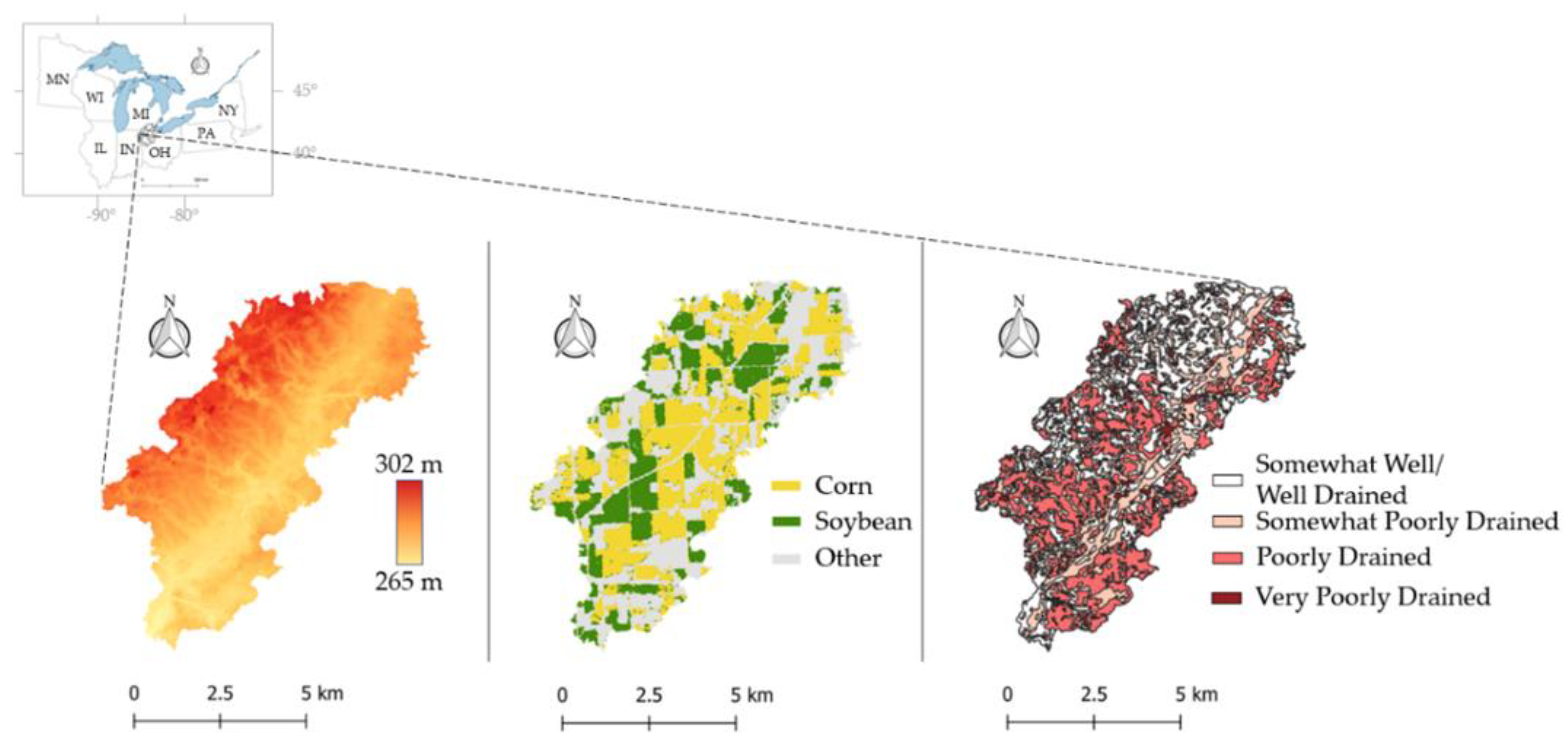
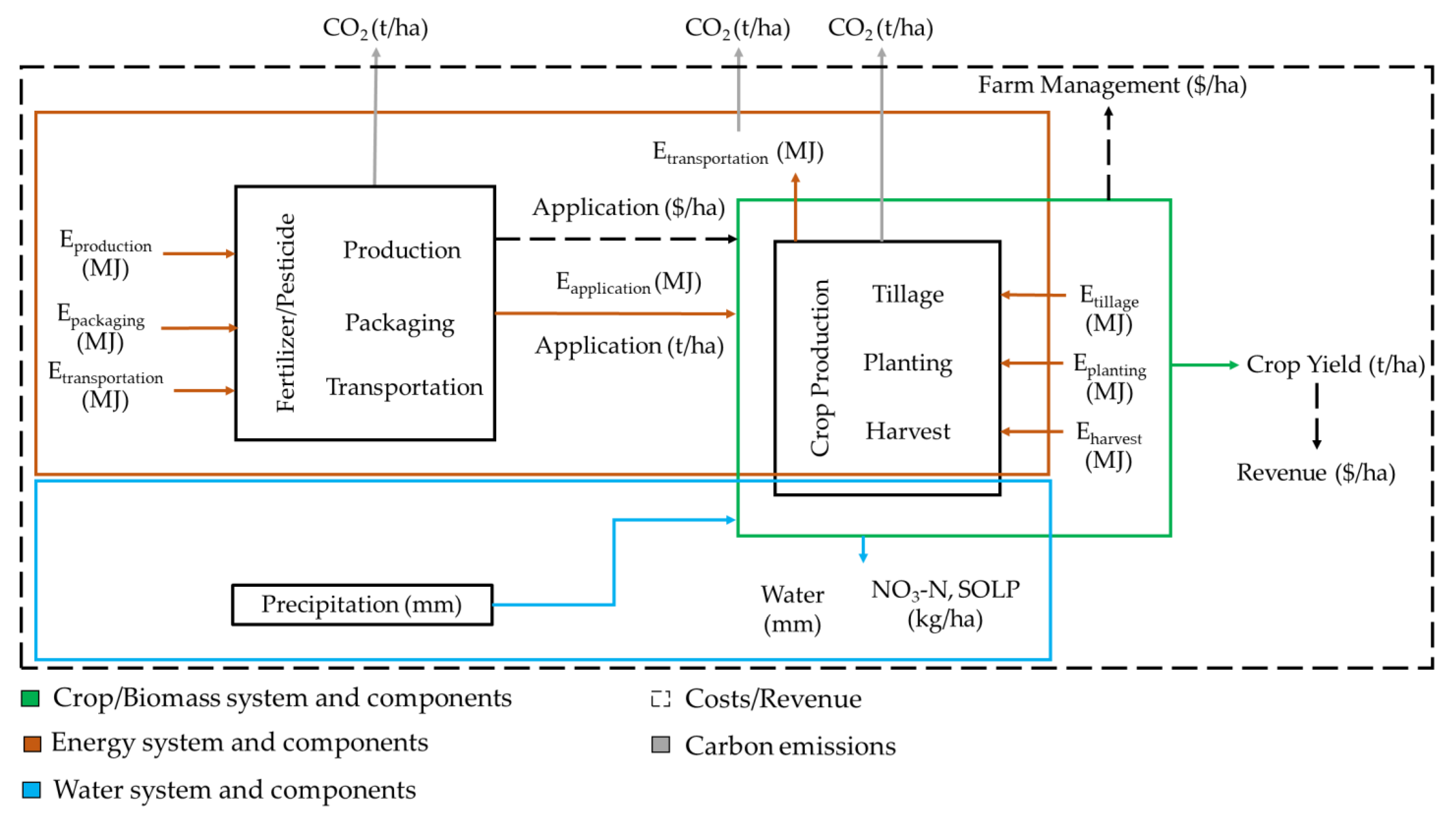
FEW Nexus System for the Matson Ditch Watershed
2. Materials and Methods
2.1. Identifying Critical Periods for Water Quantity and Quality
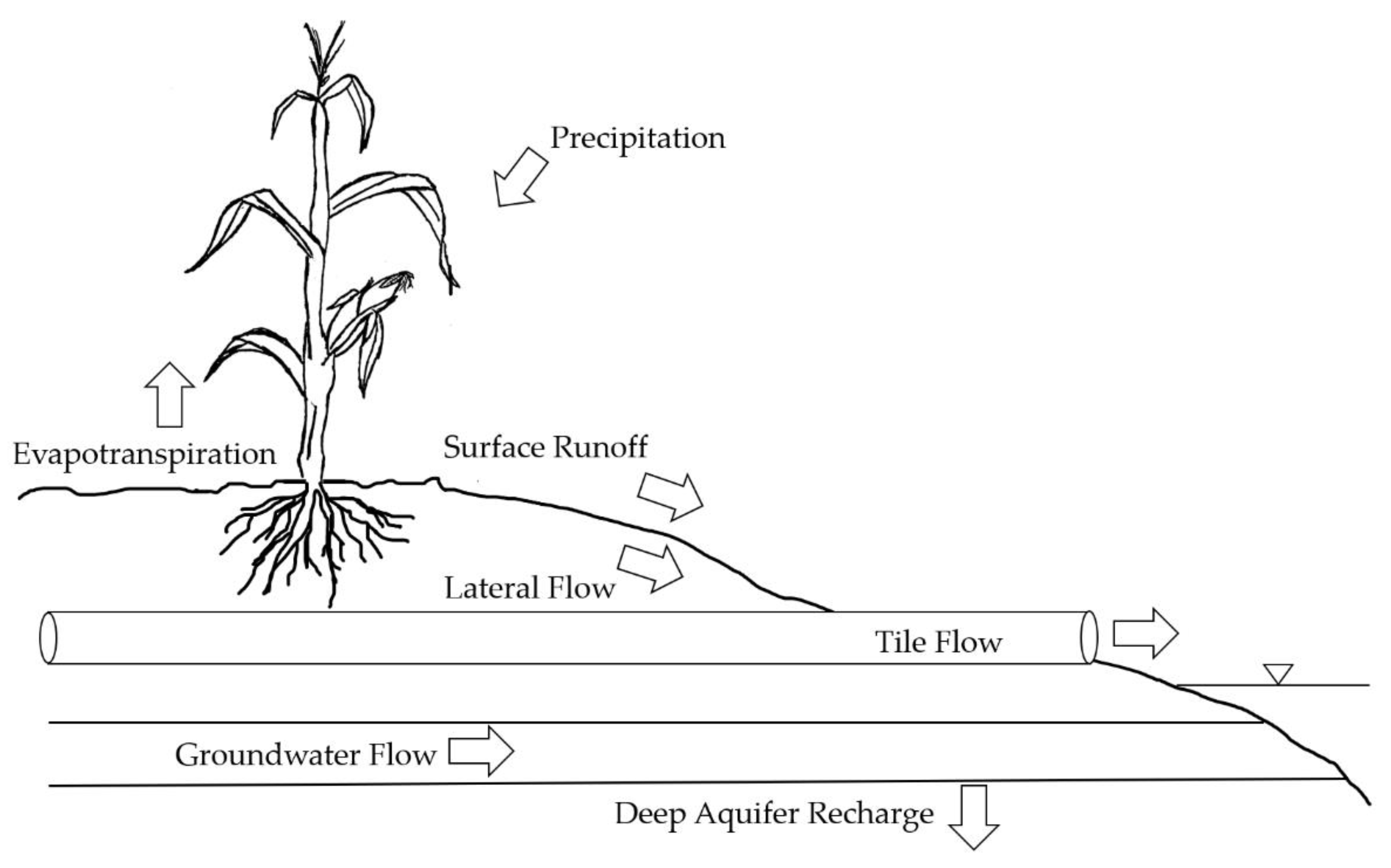
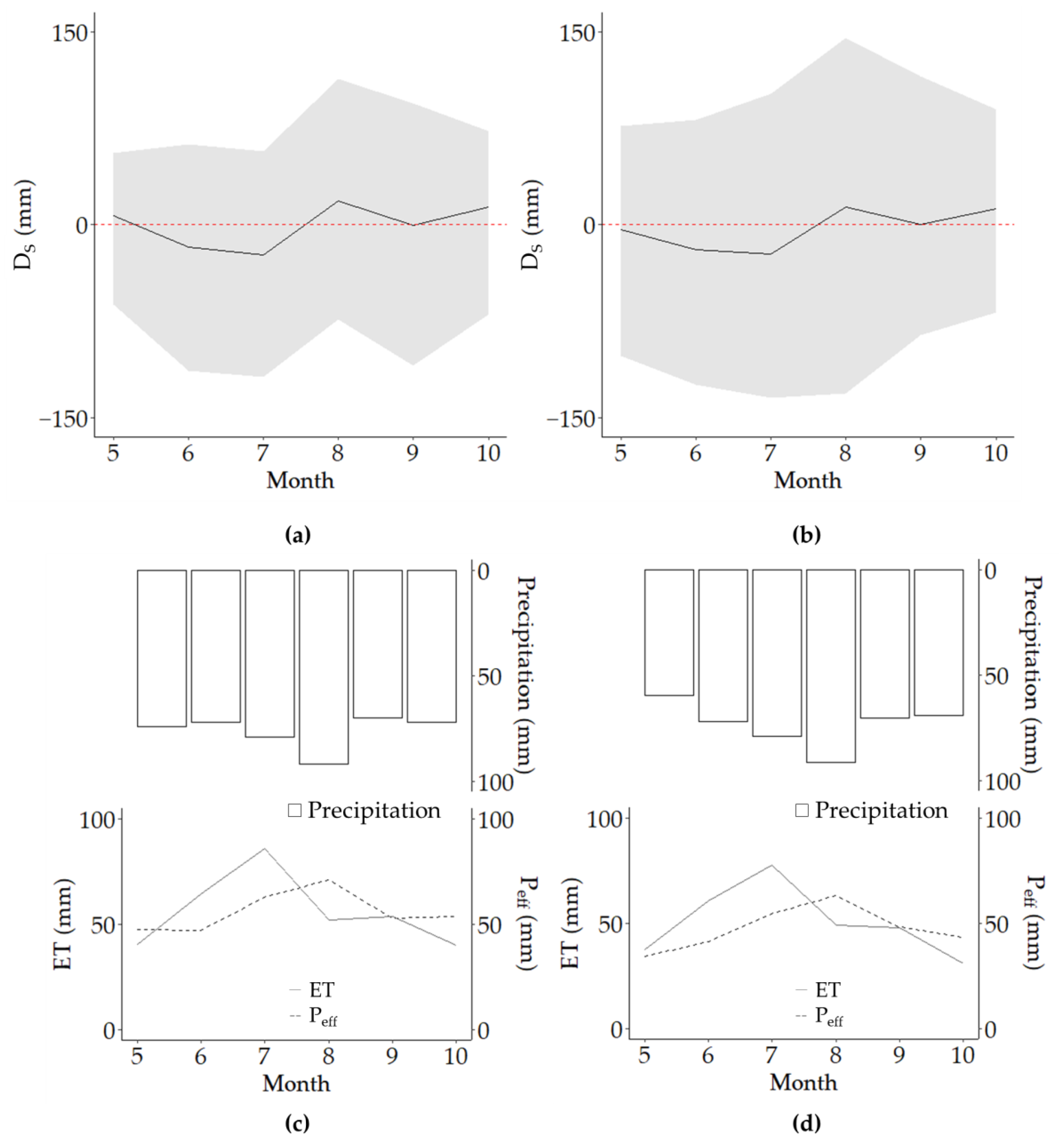
2.1.1. Water Quantity
2.1.2. Water Quality
2.2. Crop Growth
2.3. Energy Usage and Carbon Emissions
2.4. Cost Analysis in Decision-Making in the FEW Nexus
3. Results
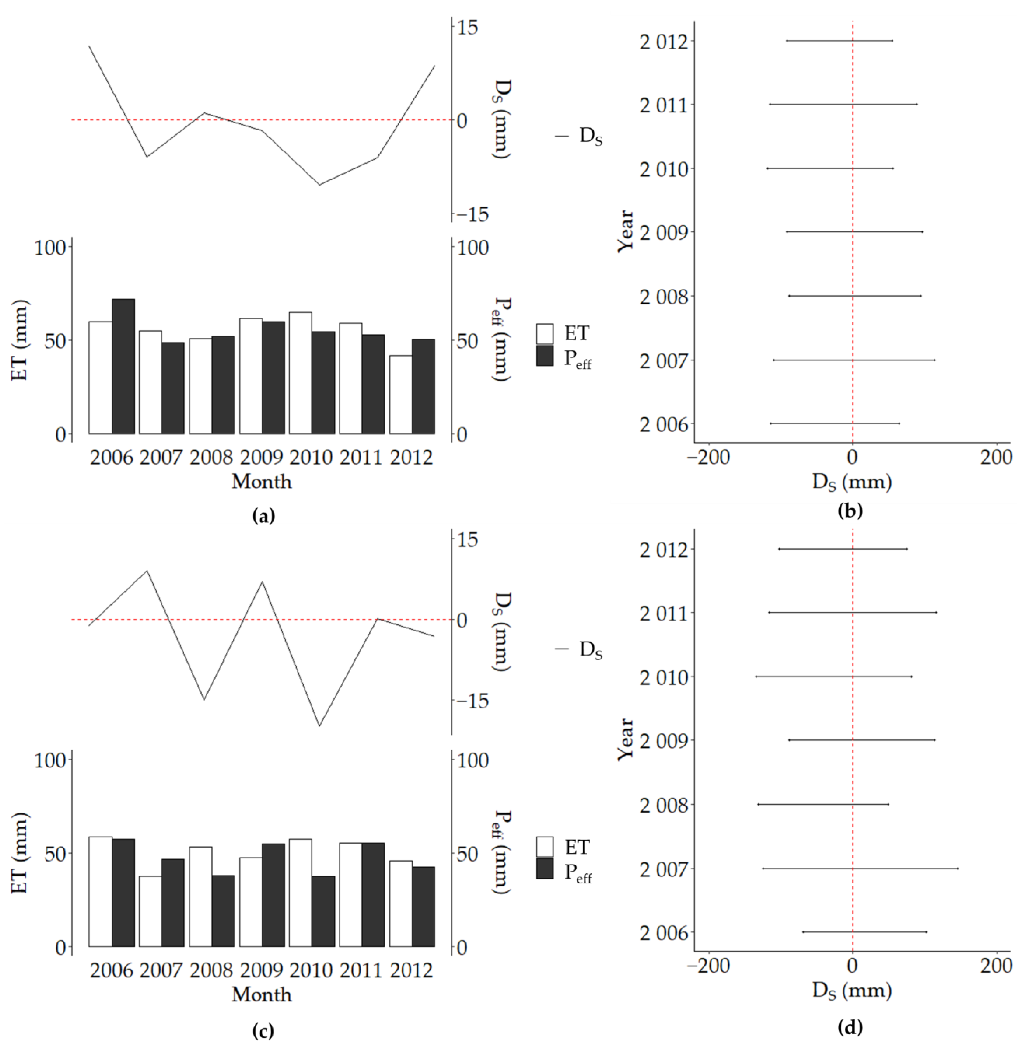
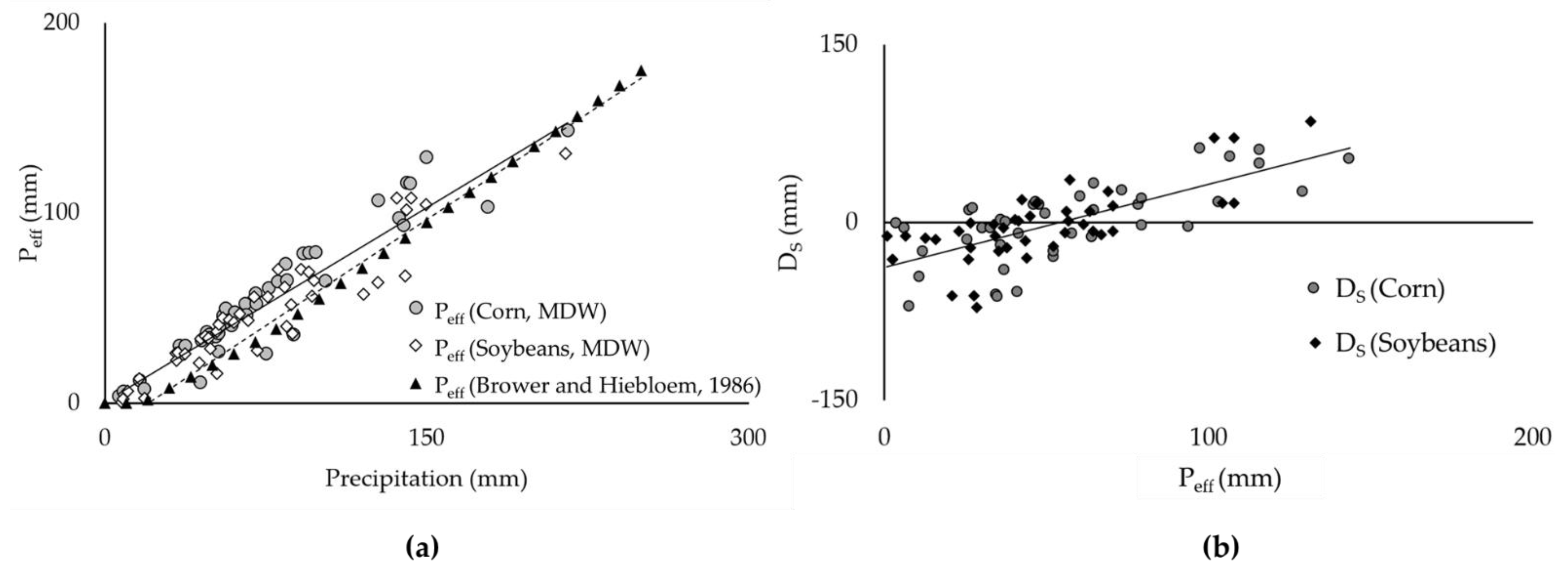
3.1. Water Quantity
3.2. Water Quality
3.3. Crop Growth
3.4. Energy Consumption and Carbon Emissions
3.5. Cost Assessment of the FEW Nexus
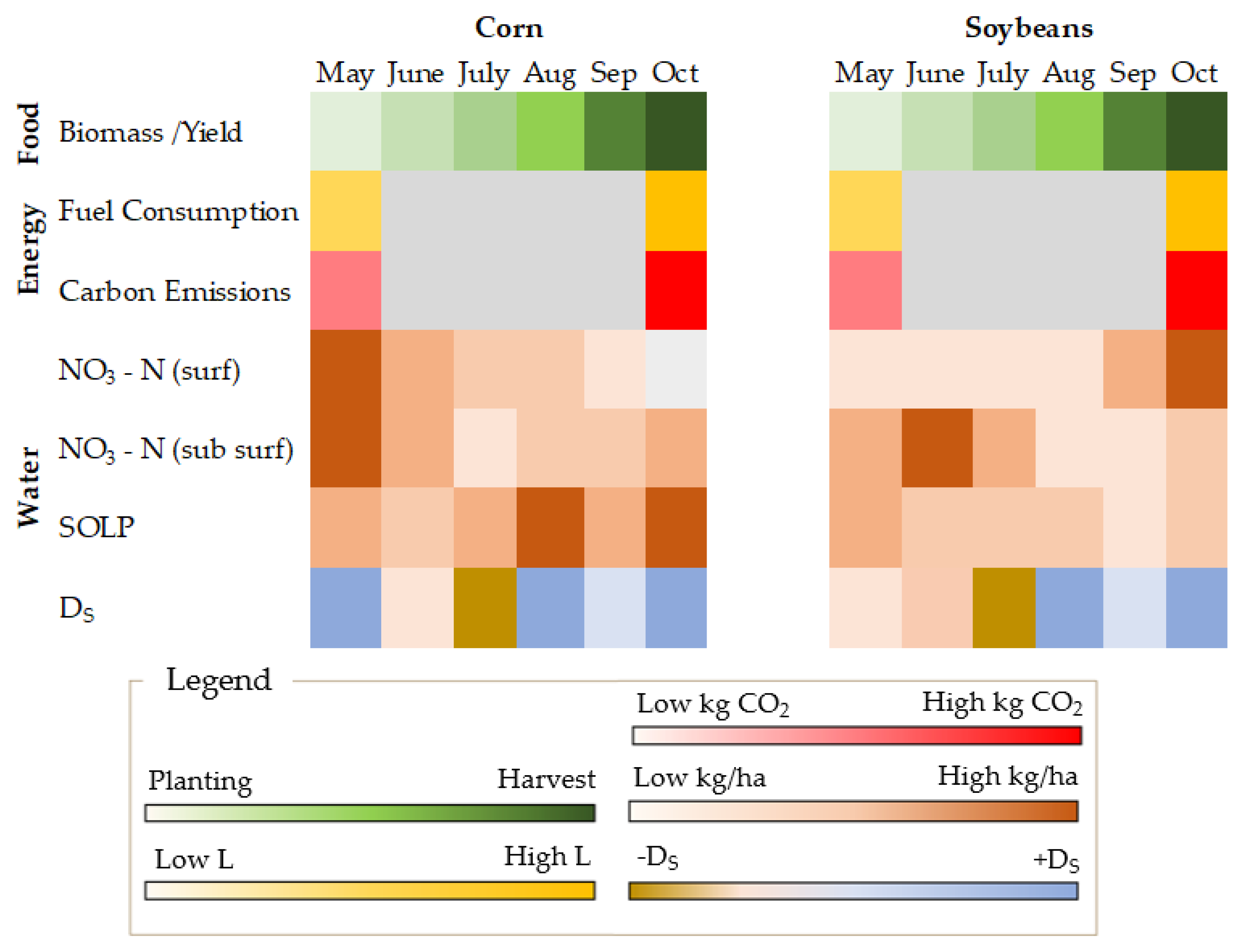
3.6. Interactions Among FEW Nexus Components in the Matson Ditch Watershed
4. Discussion
5. Conclusions
Author Contributions
Funding
Institutional Review Board Statement
Informed Consent Statement
Data Availability Statement
Acknowledgments
Conflicts of Interest
References
- Hoff, H. Understanding the Nexus. Background Paper for the Bonn2011 Conference: The Water, Energy and Food Security Nexus; Stockholm Environment Institute: Stockholm, Sweden, 2011. [Google Scholar]
- Cai, X.; Wallington, K.; Shafiee-Jood, M.; Marston, L. Understanding and managing the food-energy-water nexus—Oopportunities for water resources research. Adv. Water Resour. 2018, 111, 259–273. [Google Scholar] [CrossRef]
- Daher, B.T.; Mohtar, R.H. Water–energy–food (WEF) Nexus Tool 2.0: Guiding integrative resource planning and decision-making. Water Int. 2015, 40, 748–771. [Google Scholar] [CrossRef]
- Rao, P.; Kostecki, R.; Dale, L.; Gadgil, A. Technology and Engineering of the Water-Energy Nexus. Annu. Rev. Environ. Resour. 2017, 42, 407–437. [Google Scholar] [CrossRef]
- D’Odorico, P.; Davis, K.F.; Rosa, L.; Carr, J.A.; Chiarelli, D.; Dell’Angelo, J.; Gephart, J.; Macdonald, G.K.; Seekell, D.A.; Suweis, S.; et al. The Global Food-Energy-Water Nexus. Rev. Geophys. 2018, 56, 456–531. [Google Scholar] [CrossRef]
- Schull, V.Z.; Daher, B.; Gitau, M.W.; Mehan, S.; Flanagan, D.C. Analyzing FEW nexus modeling tools for water resources decision-making and management applications. Food Bioprod. Process. 2020, 119, 108–124. [Google Scholar] [CrossRef]
- Arnold, J.G.; Srinivasan, R.; Muttiah, R.S.; Williams, J.R. Large area hydrologic modeling and assessment part I: Model development. JAWRA 1998, 34, 73–89. [Google Scholar] [CrossRef]
- Downs, H.; Hansen, R. Estimating Farm Fuel Requirements; Farm and Ranch Series: Equipment; Colorado State University: Fort Collins, CO, USA, 1998. [Google Scholar]
- Namany, S.; Al-Ansari, T.; Govindan, R. Sustainable energy, water and food nexus systems: A focused review of decision-making tools for efficient resource management and governance. J. Clean. Prod. 2019, 225, 610–626. [Google Scholar] [CrossRef]
- United States Environmental Protection Agency (USEPA); Tetra Tech, Inc. St. Joseph River Watershed Indiana TMDLs. Available online: http://www.state.in.us/idem/nps/files/tmdl_st_joseph-lake_erie_report.pdf (accessed on 22 January 2021).
- Mehan, S. Impact of Changing Climate on Water Resources in the Western Lake Erie Basin Using SWAT. Ph.D. Thesis, Purdue University, West Lafayette, IN, USA, 2018. Available online: https://docs.lib.purdue.edu/open_access_dissertations/1512/ (accessed on 22 January 2021).
- Mehan, S.; Aggarwal, R.; Gitau, M.W.; Flanagan, D.C.; Wallace, C.W.; Frankenberger, J.R. Assessment of hydrology and nutrient losses in a changing climate in a subsurface-drained watershed. Sci. Total Environ. 2019, 688, 1236–1251. [Google Scholar] [CrossRef] [PubMed]
- Mehan, S.; Gitau, M.W.; Flanagan, D.C. Reliable Future Climatic Projections for Sustainable Hydro-Meteorological Assessments in the Western Lake Erie Basin. Water 2019, 11, 581. [Google Scholar] [CrossRef] [Green Version]
- Flanagan, D.C.; Livingston, S.J.; Huang, C.-H.; Warnemuende, E.A. Runoff and Pesticide Discharge from Agricultural Watersheds in NE Indiana; American Society of Agricultural and Biological Engineers: St. Joseph, IN, USA, 2003; p. 1. [Google Scholar] [CrossRef]
- Flanagan, D.C.; Zuercher, B.W.; Huang, C.-H. AnnAGNPS Application and Evaluation in NE Indiana; American Society of Agricultural and Biological Engineers: St. Joseph, IN, USA, 2008; p. 19. [Google Scholar] [CrossRef]
- Walthall, C.L.; Anderson, C.J.; Baumgard, L.H.; Takle, E.; Wright-Morton, L. Climate Change and Agriculture in the United States: Effects and Adaptation. Technical Bulletin. Available online: https://www.usda.gov/sites/default/files/documents/CC%20and%20Agriculture%20Report%20(02-04-2013)b.pdf (accessed on 26 January 2021).
- Johnson, B.; Whitford, F.; Hahn, L.; Flakne, D.; Frankenberger, J.; Janssen, C.; Bailey, T. Atrazine and Drinking Water: Un-derstanding the Needs of Farmers and Citizens; Purdue University Cooperative Extension Service: West Lafayette, IN, USA, 2004; p. 66. [Google Scholar]
- Sekaluvu, L.; Zhang, L.; Gitau, M. Evaluation of constraints to water quality improvements in the Western Lake Erie Basin. J. Environ. Manag. 2018, 205, 85–98. [Google Scholar] [CrossRef] [PubMed]
- United States Energy Information Agency (USEIA). Indiana State Profile and Energy Estimates. Available online: https://www.eia.gov/state/?sid=IN#tabs-1 (accessed on 21 January 2021).
- Brouwer, C.; Heibloem, M. Irrigation Water Management: Irrigation Water Needs; Training Manual; Food and Agriculture Organization (FAO) of the United Nations, Land and Water Development Division: Rome, Italy, 1986; Available online: http://www.fao.org/3/S2022E/s2022e00.htm (accessed on 25 January 2021).
- Goulding, K. Pathways and Losses of Fertilizer Nitrogen at Different Scales. In Agriculture and The Nitrogen Cycle: Assessing the Impacts of Fertilizer Use on Food Production and the Environment; Scientific Committee on Problems of the Environment: Paris, France, 2004; pp. 209–219. [Google Scholar]
- Nangia, V.; Gowda, P.H.; Mulla, D.J.; Sands, G.R. Water Quality Modeling of Fertilizer Management Impacts on Nitrate Losses in Tile Drains at the Field Scale. J. Environ. Qual. 2008, 37, 296–307. [Google Scholar] [CrossRef]
- Neitsch, S.L.; Arnold, J.G.; Kiniry, J.R.; Williams, J.R. Soil and Water Assessment Tool Theoretical Documentation Version 2009; Texas Water Resources Institute: College Station, TX, USA, 2011. [Google Scholar]
- Hanna, H.M. Fuel Required for Field Operations; Iowa State University, University Extension: Ames, IA, USA, 2001. [Google Scholar]
- United States Environmental Protection Agency (USEPA). 1.5 Liquefied Petroleum Gas Combustion. Available online: https://www3.epa.gov/ttnchie1/ap42/ch01/final/c01s05.pdf (accessed on 19 January 2021).
- United States Environmental Protection Agency (USEPA). Emission Factors for Greenhouse Gas Inventories. Available online: https://www.epa.gov/sites/production/files/2015-07/documents/emission-factors_2014.pdf (accessed on 19 January 2021).
- United States Environmental Protection Agency (USEPA). Greenhouse Gases Equivalencies Calculator-Calculations and References. Available online: https://www.epa.gov/energy/greenhouse-gases-equivalencies-calculator-calculations-and-references (accessed on 19 January 2021).
- Lal, R. Carbon emission from farm operations. Environ. Int. 2004, 30, 981–990. [Google Scholar] [CrossRef] [PubMed]
- Audsley, E.; Stacey, K.; Parsons, D.J.; Williams, A.G. Estimation of the Greenhouse Gas Emissions from Agricultural Pesticide Manufacture and Use. Available online: https://dspace.lib.cranfield.ac.uk/bitstream/handle/1826/3913/Estimation_of_the_greenhouse_gas_emissions_from_agricultural_pesticide_manufacture_and_use-2009.pdf;jsessionid=784EAECEE049B54A85B13688379064F4?sequence=1 (accessed on 26 January 2021).
- Ma, B.L.; Liang, B.C.; Biswas, D.K.; Morrison, M.J.; McLaughlin, N.B. The carbon footprint of maize production as affected by nitrogen fertilizer and maize-legume rotations. Nutr. Cycl. Agroecosyst. 2012, 94, 15–31. [Google Scholar] [CrossRef]
- Brentrup, F.; Hoxha, A.; Christensen, B. Carbon footprint analysis of mineral fertilizer production in Europe and other world regions. In Proceedings of the 10th International Conference on Life Cycle Assessment of Food (LCA Food 2016), Dublin, Ireland, 19–21 October 2016. [Google Scholar]
- Hillier, J.; Hawes, C.; Squire, G.; Hilton, A.; Wale, S.; Smith, P. The carbon footprints of food crop production. Int. J. Agric. Sustain. 2009, 7, 107–118. [Google Scholar] [CrossRef]
- Hillier, J.; Walter, C.; Malin, D.; Garcia-Suarez, T.; Mila-I-Canals, L.; Smith, P. A farm-focused calculator for emissions from crop and livestock production. Environ. Model. Softw. 2011, 26, 1070–1078. [Google Scholar] [CrossRef]
- Dobbins, C.; Langemeier, M.; Nielsen, B.; Vyn, T.; Casteel, S.; Johnson, B. Crop Cost & Return Guide. Available online: https://ag.purdue.edu/commercialag/home/resource/keyword/crop-cost-return-guide-archive/ (accessed on 19 January 2021).
- Payero, J.; Tarkalson, D.; Irmak, S.; Davison, D.; Petersen, J. Effect of timing of a deficit-irrigation allocation on corn evapotranspiration, yield, water use efficiency and dry mass. Agric. Water Manag. 2009, 96, 1387–1397. [Google Scholar] [CrossRef] [Green Version]
- Suyker, A.E.; Verma, S.B. Evapotranspiration of irrigated and rainfed maize–soybean cropping systems. Agric. For. Meteorol. 2009, 149, 443–452. [Google Scholar] [CrossRef] [Green Version]
- Stone, L.R. Crop water use requirements and water use efficiency. In Proceedings of the 15th annual Central Plains Irrigation Conference and Exposition proceedings, Colby, KS, USA, 4–5 February 2003. [Google Scholar]
- Widhalm, M. Corn Growth Stages with Estimated Calendar Days and Growing-Degree Units. Available online: https://mygeohub.org/resources/879/download/Corn-growth-stage-day-and-GDU-calendar10.pdf (accessed on 22 January 2021).
- Casteel, S. Soybean Physiology: How Well Do You Know Soybeans. Available online: https://www.agry.purdue.edu/ext/soybean/arrivals/10soydevt.pdf (accessed on 22 January 2021).
- Ritchie, J.T. Model for predicting evaporation from a row crop with incomplete cover. Water Resour. Res. 1972, 8, 1204–1213. [Google Scholar] [CrossRef] [Green Version]
- Widhalm, M.; Hamlet, A.; Byun, K.; Robeson, S.; Baldwin, M.; Staten, P.; Chiu, C.-M.; Coleman, J.; Hall, B.; Hoogewind, K. Indiana’s Past & Future Climate: A Report from the Indiana Climate Change Impacts Assessment; Purdue University: West Lafayette, IN, USA, 2018. [Google Scholar]
- Byun, K.; Hamlet, A.F. Projected changes in future climate over the Midwest and Great Lakes region using downscaled CMIP5 ensembles. Int. J. Clim. 2018, 38, e531–e553. [Google Scholar] [CrossRef]
- Hatfield, J.L.; Wright-Morton, L.; Hall, B. Vulnerability of grain crops and croplands in the Midwest to climatic variability and adaptation strategies. Clim. Chang. 2018, 146, 263–275. [Google Scholar] [CrossRef] [Green Version]
- United States Environmental Protection Agency (USEPA). Adapting to Climate Change: Midwest. Office of Policy. Available online: https://www.epa.gov/sites/production/files/2016-07/documents/midwest_fact_sheet.pdf (accessed on 25 January 2021).
- United States Environmental Protection Agency (USEPA). Climate Impacts in the Midwest. Available online: https://19january2017snapshot.epa.gov/climate-impacts/climate-impacts-midwest_.html (accessed on 5 July 2020).
- O’Neal, M.R.; Nearing, M.; Vining, R.C.; Southworth, J.; Pfeifer, R.A. Climate change impacts on soil erosion in Midwest United States with changes in crop management. Catena 2005, 61, 165–184. [Google Scholar] [CrossRef]
- Wuebbles, D.J.; Hayhoe, K. Climate Change Projections for the United States Midwest. Mitig. Adapt. Strat. Glob. Chang. 2004, 9, 335–363. [Google Scholar] [CrossRef] [Green Version]
- Licht, M.; Sotirios, A. Integrated Crop Management. Influence of Drought on Corn and Soybean; Iowa State University, University Extension: Ames, IA, USA, 2017; Available online: https://crops.extension.iastate.edu/cropnews/2017/07/influence-drought-corn-and-soybean (accessed on 25 January 2021).
- Wallace, C.W. Simulation of Conservation Practice Effects on Water Quality Under Current and Future Climate Scenarios. Ph.D. Thesis, Purdue University, West Lafayette, IN, USA, 2016. Available online: https://docs.lib.purdue.edu/open_access_dissertations/724/ (accessed on 22 January 2021).
- United States Energy Information Agency (USEIA). How Much Carbon Dioxide is Produced when Different Fuels are Burned? Available online: https://www.eia.gov/tools/faqs/faq.php?id=73&t=11 (accessed on 19 January 2021).
- Hall, C.A.; Dale, B.E.; Pimentel, D. Seeking to Understand the Reasons for Different Energy Return on Investment (EROI) Estimates for Biofuels. Sustainability 2011, 3, 2413–2432. [Google Scholar] [CrossRef] [Green Version]
- Kim, S.; Dale, B.E. Life cycle assessment of various cropping systems utilized for producing biofuels: Bioethanol and biodiesel. Biomass Bioenergy 2005, 29, 426–439. [Google Scholar] [CrossRef]
- Pimentel, D.; Patzek, T.W. Ethanol Production Using Corn, Switchgrass, and Wood; Biodiesel Production Using Soybean and Sunflower. Nat. Resour. Res. 2005, 14, 65–76. [Google Scholar] [CrossRef]
- Mondesir, R. A Historical Look at Soybean Price Increases: What Happened Since the Year 2000? Available online: https://stats.bls.gov/opub/btn/volume-9/pdf/a-historical-look-at-soybean-price-increases-what-happened-since-the-year-2000.pdf (accessed on 22 January 2021).
- National Research Council (NRC). Water Implications of Biofuels Production in the United States; National Academies Press: Washington, DC, USA, 2008; Available online: https://www.nap.edu/catalog/12039/water-implications-of-biofuels-production-in-the-united-states (accessed on 25 January 2021).
- Wishin, A.R. Soy and the City: The Protection of Indiana’s Agricultural Land in Light of Biofuel Issues. Valpso. Univ. Law Rev. 2008, 42. Available online: https://scholar.valpo.edu/vulr/vol42/iss3/7 (accessed on 26 January 2021).
- Hochman, G.; Kaplan, S.; Rajagopal, D.; Zilberman, D. Biofuel and Food-Commodity Prices. Agriculture 2012, 2, 272–281. [Google Scholar] [CrossRef] [Green Version]
- Langemeier, M. Relative Profitability of Corn and Soybean Production in Indiana. Available online: https://ag.purdue.edu/commercialag/Documents/Resources/Mangagement-Strategy/Crop-Economics/2017_04_04_Langemeier_Relative_Profitability.pdf (accessed on 22 January 2021).
- Loux, M.M.; Doohan, D.; Dobbels, A.F.; Johnson, W.G.; Young, B.G.; Legleiter, T.R.; Hager, A. Weed Control Guide for Ohio, Indiana and Illinois. Available online: https://farmdoc.illinois.edu/wp-content/uploads/2014/12/2015-Weed-Control-Guide.pdf (accessed on 25 January 2021).
- Rothausen, S.G.S.A.; Conway, D. Greenhouse-gas emissions from energy use in the water sector. Nat. Clim. Chang. 2011, 1, 210–219. [Google Scholar] [CrossRef]
- Reinhart, B.D.; Frankenberger, J.R.; Hay, C.H.; Helmers, M.J. Simulated water quality and irrigation benefits from drainage water recycling at two tile-drained sites in the U.S. Midwest. Agric. Water Manag. 2019, 223, 105699. [Google Scholar] [CrossRef]
- Gitau, M.W.; Veith, T.L.; Gburek, W.J. Farm–level optimization of bmp placement for cost–effective pollution reduction. Trans. ASAE 2004, 47, 1923–1931. [Google Scholar] [CrossRef]
- Ali, M.H.; Mubarak, S. Effective Rainfall Calculation Methods for Field Crops: An Overview, Analysis and New Formulation. Asian Res. J. Agric. 2017, 7, 1–12. [Google Scholar] [CrossRef]
- Cain, Z.; Lovejoy, S. The Economic and Environmental Effect of Adding Conservation Buffer Areas in the Matson Ditch Wa-Tershed; Purdue University: West Lafayette, IN, USA, 2006. [Google Scholar]
- Mueller, D.K.; Spahr, N.E. Nutrients in Streams and Rivers Across the Nation. Sci. Investig. Rep. 2006, 5107, 2328. [Google Scholar]
- Vitousek, P.M.; Hättenschwiler, S.; Olander, L.; Allison, S. Nitrogen and Nature. AMBIO 2002, 31, 97–101. [Google Scholar] [CrossRef] [PubMed]
- Chaffin, J.D.; Bridgeman, T.B.; Bade, D.L. Nitrogen Constrains the Growth of Late Summer Cyanobacterial Blooms in Lake Erie. Adv. Microbiol. 2013, 3, 16–26. [Google Scholar] [CrossRef] [Green Version]
- Mueller, D.K.; Helsel, D.R. Nutrients in the Nation’s Waters—Too Much of a Good Thing? US Government Printing Office: Washington, DC, USA, 1996; Volume 1136.
- Kerr, J.M.; DePinto, J.V.; McGrath, D.; Sowa, S.P.; Swinton, S.M. Sustainable management of Great Lakes watersheds dominated by agricultural land use. J. Great Lakes Res. 2016, 42, 1252–1259. [Google Scholar] [CrossRef] [Green Version]
- Bridgeman, T.B.; Chaffin, J.D.; Kane, D.D.; Conroy, J.D.; Panek, S.E.; Armenio, P.M. From River to Lake: Phosphorus partitioning and algal community compositional changes in Western Lake Erie. J. Great Lakes Res. 2012, 38, 90–97. [Google Scholar] [CrossRef]
- Michalak, A.M.; Anderson, E.J.; Beletsky, D.; Boland, S.; Bosch, N.S.; Bridgeman, T.B.; Chaffin, J.D.; Cho, K.; Confesor, R.; Daloğlu, I.; et al. Record-setting algal bloom in Lake Erie caused by agricultural and meteorological trends consistent with expected future conditions. Proc. Natl. Acad. Sci. USA 2013, 110, 6448–6452. [Google Scholar] [CrossRef] [PubMed] [Green Version]
- Daloğlu, I.; Cho, K.H.; Scavia, D. Evaluating Causes of Trends in Long-Term Dissolved Reactive Phosphorus Loads to Lake Erie. Environ. Sci. Technol. 2012, 46, 10650–10666. [Google Scholar] [CrossRef]
- Mijares, V.; Gitau, M.; Johnson, D.R. A Method for Assessing and Predicting Water Quality Status for Improved Decision-Making and Management. Water Resour. Manag. 2018, 33, 509–522. [Google Scholar] [CrossRef]
- Gobler, C.J.; Burkholder, J.M.; Davis, T.W.; Harke, M.J.; Johengen, T.; Stow, C.A.; Van de Waal, D.B. The dual role of nitrogen supply in controlling the growth and toxicity of cyanobacterial blooms. Harmful Algae 2016, 54, 87–97. [Google Scholar] [CrossRef]
- Davis, T.W.; Berry, D.L.; Boyer, G.L.; Gobler, C.J. The effects of temperature and nutrients on the growth and dynamics of toxic and non-toxic strains of Microcystis during cyanobacteria blooms. Harmful Algae 2009, 8, 715–725. [Google Scholar] [CrossRef]
- Heisler, J.; Glibert, P.; Burkholder, J.; Anderson, D.; Cochlan, W.; Dennison, W.; Dortch, Q.; Gobler, C.; Heil, C.; Humphries, E.; et al. Eutrophication and harmful algal blooms: A scientific consensus. Harmful Algae 2008, 8, 3–13. [Google Scholar] [CrossRef] [PubMed] [Green Version]
- Shiferaw, B.A.; Okello, J.; Reddy, R.V. Adoption and adaptation of natural resource management innovations in smallholder agriculture: Reflections on key lessons and best practices. Environ. Dev. Sustain. 2007, 11, 601–619. [Google Scholar] [CrossRef]
- Zhang, W. Agricultural land management and downstream water quality: Insights from Lake Erie. In Proceedings of the Integrated Crop Management Conference, Iowa State University, Ames, IN, USA, 1 December 2016. [Google Scholar]
- Burnett, E.A.; Wilson, R.S.; Roe, B.; Howard, G.; Irwin, E.; Zhang, W.; Martin, J. Farmers, Phosphorus and Water Quality: Part II. A Descriptive Report of Beliefs, Attitudes and Best Management Practices in the Maumee Watershed of the Western Lake Erie Basin; The Ohio State University, School of Environment & Natural Resources: Columbus, OH, USA, 2015; Available online: https://www2.econ.iastate.edu/faculty/zhang/publications/outreach-articles/farmers-phosphorus-and-water-quality-2015-burnett.pdf (accessed on 25 January 2021).
- Mannan, M.; Al-Ansari, T.; Mackey, H.R.; Al-Ghamdi, S.G. Quantifying the energy, water and food nexus: A review of the latest developments based on life-cycle assessment. J. Clean. Prod. 2018, 193, 300–314. [Google Scholar] [CrossRef]
- Ikerd, J. Marketing Strategies for New Farmers. Available online: http://web.missouri.edu/~ikerdj/papers/SFT-New%20Farm%20Marketing%20(508).htm#:~:text=Grain%20farmers%20can%20sell%20at,buyers%20at%20different%20market%20locations (accessed on 22 January 2021).


| Year | Yield (t/ha) | |||
|---|---|---|---|---|
| Corn | Soybeans | |||
| Observed | Simulated | Observed | Simulated | |
| 2006 | 9.2 | 6.5 | 3.0 | 1.5 |
| 2007 | 9.2 | 4.5 | 3.0 | 3.8 |
| 2008 | 7.6 | 6.5 | 2.1 | 0.5 |
| 2009 | 9.4 | 8.1 | 3.0 | 1.5 |
| 2010 | 7.7 | 8.2 | 2.6 | 4.2 |
| 2011 | 7.8 | 5.8 | 2.7 | 3.7 |
| 2012 | 5.7 | 5.6 | 3.0 | 2.7 |
| Crop | Date | Management Operation | Rate |
|---|---|---|---|
| Corn | 22 April | Nitrogen Application (as Anhydrous Ammonia) | 176.0 kg/ha |
| 22 April | (P2O5) Application (DAP/MAP) | 54.0 kg/ha | |
| 22 April | Pesticide Application | 2.2 kg/ha | |
| 6 May | Tillage–Offset Disk (60% mixing) | ||
| 6 May | Planting–Row Planter, double disk openers | ||
| 10 October | Harvest | ||
| Soybeans | 10 May | (P2O5) Application (DAP/MAP) | 40.0 kg/ha |
| 24 May | No–tillage planting–Drills | ||
| 7 October | Harvest | ||
| 20 October | Tillage, Chisel (30% mixing) |
| Fuel Required (L/ha) | ||||||
| Crop | Fuel Type | Downs and Hansen (1998); Hanna (2001) [8,23] | Lal (2004) [28] † | |||
| Corn | Diesel | (36.7, 58.9) | (36.9, 69.3) | |||
| Gasoline | (40.8 *, 42.1) | (46.1, 85.5) | ||||
| LP Gas | (54.9 *, 70.8) | (90.8, 170.3) | ||||
| Soybeans | Diesel | (26.2, 49.1) | (24.7, 42.8) | |||
| Gasoline | (29.1 *, 35.0) | (30.9, 53.4) | ||||
| LP Gas | (39.2 *, 59.0) | (61.6, 102.0) | ||||
| Carbon Emissions (kg CO2/L) | ||||||
| Fuel Type | Daher (2012) [3] | Lal (2004) [28] | USEPA (2008) [25] | USEPA (2014) [26] | USEIA (2019) [50] | USEPA (2020) [27] |
| Diesel | 2.6 | 0.8 ** | 2.7 | 2.7 | 2.7 | |
| Gasoline | 2.4 | 0.6 ** | 2.3 | 2.3 | 2.3 | |
| LP Gas | 2.3 | 0.3 ** | 1.7 | 1.5 | ||
| Estimates | Chemical | References | ||
|---|---|---|---|---|
| Anhydrous Ammonia | P2O5 (DAP/MAP) | Atrazine | ||
| Total MJ/kg ai | 63 | 18 | 208 | [29,51,52] |
| 67 | 17.4 | 189 | [29,51,52] | |
| - | - | 190 | [29,53] | |
| Total kg CO2/kg ai | (0.9–1.8) | (0.1–0.3) | 3.8 | [28] |
| 4.8 | 0.73 | 23.1 | [30] | |
| 2.52 | 0.73 | - | [31] | |
| 1.3 | 0.2 | 6.3 | [32] | |
| 1.74 | 0.33 | - | [33] | |
| Earnings/Losses per ha | ||
|---|---|---|
| Year | Corn | Soybeans |
| 2003 | (USD −126.67, USD −65.04) | (USD −212.00, USD −152.69) |
| 2004 | (USD −116.83, USD −97.38) | (USD −123.70, USD 12.17) |
| 2005 | (USD −196.55, USD −166.66) | (USD −236.77, USD −171.57) |
| 2006 | (USD −199.37, USD −184.03) | (USD −207.62, USD −125.37) |
| 2007 | (USD 216.90, USD 559.50) | (USD 17.02, USD 240.80) |
| 2008 | (USD 151.87, USD 687.56) | (USD 211.39, USD 609.74) |
| 2009 | (USD −297.86, USD 45.09) | (USD −290.97, USD −115.02) |
| 2010 | (USD −52.24, USD 317.40) | (USD −142.46, USD 87.85) |
| 2011 | (USD 259.76, USD 838.84) | (USD 149.81, USD 571.39) |
| 2012 | (USD 72.80, USD 614.92) | (USD −20.64, USD 310.49) |
Publisher’s Note: MDPI stays neutral with regard to jurisdictional claims in published maps and institutional affiliations. |
© 2021 by the authors. Licensee MDPI, Basel, Switzerland. This article is an open access article distributed under the terms and conditions of the Creative Commons Attribution (CC BY) license (http://creativecommons.org/licenses/by/4.0/).
Share and Cite
Schull, V.Z.; Mehan, S.; Gitau, M.W.; Johnson, D.R.; Singh, S.; Sesmero, J.P.; Flanagan, D.C. Construction of Critical Periods for Water Resources Management and Their Application in the FEW Nexus. Water 2021, 13, 718. https://doi.org/10.3390/w13050718
Schull VZ, Mehan S, Gitau MW, Johnson DR, Singh S, Sesmero JP, Flanagan DC. Construction of Critical Periods for Water Resources Management and Their Application in the FEW Nexus. Water. 2021; 13(5):718. https://doi.org/10.3390/w13050718
Chicago/Turabian StyleSchull, Val Z., Sushant Mehan, Margaret W. Gitau, David R. Johnson, Shweta Singh, Juan P. Sesmero, and Dennis C. Flanagan. 2021. "Construction of Critical Periods for Water Resources Management and Their Application in the FEW Nexus" Water 13, no. 5: 718. https://doi.org/10.3390/w13050718