Means and Extremes: Evaluation of a CMIP6 Multi-Model Ensemble in Reproducing Historical Climate Characteristics across Alberta, Canada

Abstract

This study evaluates General Circulation Models (GCMs) participating in the Coupled Model Intercomparison Project Phase 6 (CMIP6) for their ability in simulating historical means and extremes of daily precipitation (P), and daily maximum (Tmax), and minimum temperature (Tmin). Models are evaluated against hybrid observations at 2255 sub-basins across Alberta, Canada using established statistical metrics for the 1983–2014 period. Three extreme indices including consecutive wet days (CWD), summer days (SD), and warm nights (WN) are defined based on the peak over the threshold approach and characterized by duration and frequency. The tail behaviour of extremes is evaluated using the Generalized Pareto Distribution. Regional evaluations are also conducted for four climate sub-regions across the study area. For both mean annual precipitation and mean annual daily temperature, most GCMs more accurately reproduce the observations in northern Alberta and follow a gradient toward the south having the poorest representation in the western mountainous area. Model simulations show statistically better performance in reproducing mean annual daily Tmax than Tmin, and in reproducing annual mean duration compared to the frequency of extreme indices across the province. The Kernel density curves of duration and frequency as simulated by GCMs show closer agreement to that of observations in the case of CWD. However, it is slightly (completely) overestimated (underestimated) by GCMs for warm nights (summer days). The tail behaviour of extremes indicates that GCMs may not incorporate some local processes such as the convective parameterization scheme in the simulation of daily precipitation. Model performances in each of the four sub-regions are quite similar to their performances at the provincial scale. Bias-corrected and downscaled GCM simulations using a hybrid approach show that the downscaled GCM simulations better represent the means and extremes of P characteristics compared to Tmax and Tmin. There is no clear indication of an improved tail behaviour of GPD based on downscaled simulations.

1. Introduction

Simulations from the state-of-the-art General Circulation Models (GCMs) are becoming available for analysis and being included in the 6th assessment report (AR6) of the Intergovernmental Panel on Climate Change (IPCC) through the Coupled Model Intercomparison Project Phase 6 (CMIP6) [1]. One of the major differences between CMIP5 [2] and CMIP6 is the set of future scenarios used to project climate evolution. The CMIP6 implemented scenarios are based on socioeconomic trajectories (i.e., shared socioeconomic pathways or SSP) [3], which work in harmony with the Representative Concentration Pathways (RCP) [4] from CMIP5. The development of the CMIP6 phase is to overcome and improve the limitations identified in CMIP5, namely as identifying (and interpreting) systematic errors in simulations, improving the estimation of radiative forcings, identifying the response of climate to aerosol forcing, and improving the representation of impacts of land use changes on climate [1,5]. Multiple business-as-usual scenarios are available in CMIP6, and simulations from climate models are focused on biases, processes, and feedbacks. More reliable climate projections motivates the research community to address climate change impacts on various processes involved in terrestrial and aquatic environments at numerous geospatial scales. Therefore, evaluating the performance of CMIP6 models in reproducing the historical mean and extreme climate characteristics at a local scale is crucial and is an integral part of the confidence-building exercise for climate change projections.

Climate varies across different geospatial regions due to the uneven distribution of radiative heating, the individual responses of the earth and environmental systems (e.g., atmosphere, ocean, and land surface) as well as their interactions, and the physical characteristics of the regions [6]. Furthermore, the response of these systems to climate forcings is partly governed by feedback processes that are continuously variable across regions. Therefore, the amplitude of climate change is varied from one region to another. For example, annual mean precipitation has decreased in much of the West, Southwest, and Southeast of the United States and increased in most of the Northern and Southern Plains, Midwest, and Northeast areas from 1986–2015 relative to 1901–1960 [7]. In Canada, the annual mean precipitation has increased with larger relative increases over northern Canada (region of 60º north latitude) during the 1948–2012 period [8]. One of the earliest and consistent global warming theories suggests that regions in high latitudes would experience greater temperature increases than their lower latitude counterparts [9]. In fact, the annual average temperature has increased by 0.7 °C over the contiguous United States, i.e., low to mid-latitudes, during the 1986–2016 period relative to 1901–1960 [10], while in Canada (high latitudes), the annual average temperature has increased by 1.7 °C at the country scale and 2.3 °C in northern Canada between 1948 and 2016 [8]. Furthermore, topography plays a vital role in the formation and changes in precipitation and temperature patterns and their distribution. Higher uncertainties in reproducing extreme climate appeared in regions with rapid topographical change [11]. Therefore, testing the ability of climate models to reproduce the historical climate over a range of geospatial domains is important and will benefit the users of climate model output in aspects such as hydrological modelling and natural hazard risk assessment.

The impacts of climate extremes on humans and natural ecosystems are profound at the current moderate warming level [12], and they are often the most significant and costliest impacts on these ecosystems [13,14,15]. Extreme precipitation events can generate devastating floods with severe risks on human lives, properties, and critical infrastructure [16,17,18]. Similarly, extremely high temperatures can result in heat waves and catastrophic consequences that include deaths from hyperthermia [13,19], crop failures, and reduced food security [20]. For example, an uncommon multi-day extreme precipitation event combined with above-normal spring snowmelt in the Canadian Rockies and substantial antecedent rainfall [21,22], resulted in the 2013 Calgary flood in Alberta, Canada—the largest flood in the Canadian history. This flood resulted in four deaths, displaced tens of thousands of people, and caused an estimated $6 billion in damage [23]. Further, drought conditions that were experienced during eight consecutive seasons from September 2000 to August 2002 with below-normal precipitation, was one of the most severe droughts on record in the Canadian Prairies [24,25]. During this drought, agricultural production dropped by $3.6 billion in the year 2000–2001, and the gross domestic production declined by $5.8 billion [26]. These observations signify the importance of estimating the probability of such extreme events accurately. The probability estimation depends on the tail behaviour of the distribution that models extreme events [27,28]. For instance, a heavy tail implies a higher probability of more frequent extreme events [29,30]. Therefore, correct representation of the tail characteristics, as described by the shape parameter of the extreme value distribution [31], avoids serious under- or overestimation of occurrence probabilities of extreme events and ensures a proper assessment of future climate risks and uncertainties [32]. Hence, analyzing the tail behaviour of historical climate extreme events using CMIP6 data can provide important information and allows thorough investigation of CMIP6 model capabilities in projection of climate change and their impacts.

A wide range of research has been conducted using the extreme indices of temperature and precipitation developed by the Expert Team on Climate Change Detection and Indices (ETCCDI). Karl et al. [33] and Frich et al. [34] provided a comprehensive overview of ETCCDI developed temperature and precipitation extreme indices. Alexander et al. [34] and Donat et al. [35] also supported this effort by developing a gridded dataset of climate indices (e.g., HadEX and HadEX2) based on a reasonably dense global coverage. Most of these climate indices describe relatively moderate climate extremes with reoccurrence times of at least once a year [36]. However, the analysis of extreme climate events involves several difficulties compared to the analysis of mean events, including valid definitions and formulation of extremes [37,38]. This study focuses on climate extremes based on daily temperature and precipitation, such as the duration and frequency of extreme wet and hot days.

Given that CMIP6 climate projections have only recently been released, only limited research has been conducted to evaluate their simulations in reproducing means and extreme climate conditions [39,40,41,42,43,44,45,46,47]. These studies mainly compared the CMIP6 simulations with CMIP5 and found that CMIP6 medians are generally much closer to the observations [40]. They also found a general improvement in the simulation of climate extremes of CMIP6 models, and there is some indication that CMIP6 has reduced some of the warm biases [40,42]. They attributed the difference between the CMIP5 and CMIP6 simulated precipitation and temperature-based results to the sophistication of CMIP6 models that included representation of aerosol effects, new cloud fraction scheme, an improved snow-albedo scheme, model resolution, and parameterization improvements [42,44]. While these studies provide important information on the performance of CMIP6 models at global scale, they lack a detailed investigation at a local scale, where most decisions are made and actual impact assessments are performed.

The purpose of this paper is to evaluateCMIP6 models in reproducing local historical climate variables, such as means and extremes, over a large geographic region with diverse geospatial, topographic, and climatic characteristics. The specific objectives are to (1) evaluate how precisely the simulations of CMIP6 models reproduce the historical mean daily precipitation and temperature, (2) evaluate how precisely the simulations of CMIP6 models reproduce the tail behaviour of their probability distributions, and (3) investigate whether a correlation exists between the bias in tails and geospatial regions. We also applied a hybrid bias correction and statistical downscaling technique to check whether the performance of GCMs could be improved for the aforementioned objectives. To achieve these objectives, we focused our analyses in the province of Alberta, Canada, which is characterized by heterogeneous soil, land use, topographic, and climatic characteristics and has also been exposed to historical extreme precipitation events and droughts. Our study lays the foundation for future research based on CMIP6 data and enhance our understanding of climate change impact assessments that explore the probability of climate-related threats. Note that the presence of annual cycle or season-specific behaviour in the time series are not considered for the evaluation purposes and are beyond the scope of the study.

2. Study Area and Data

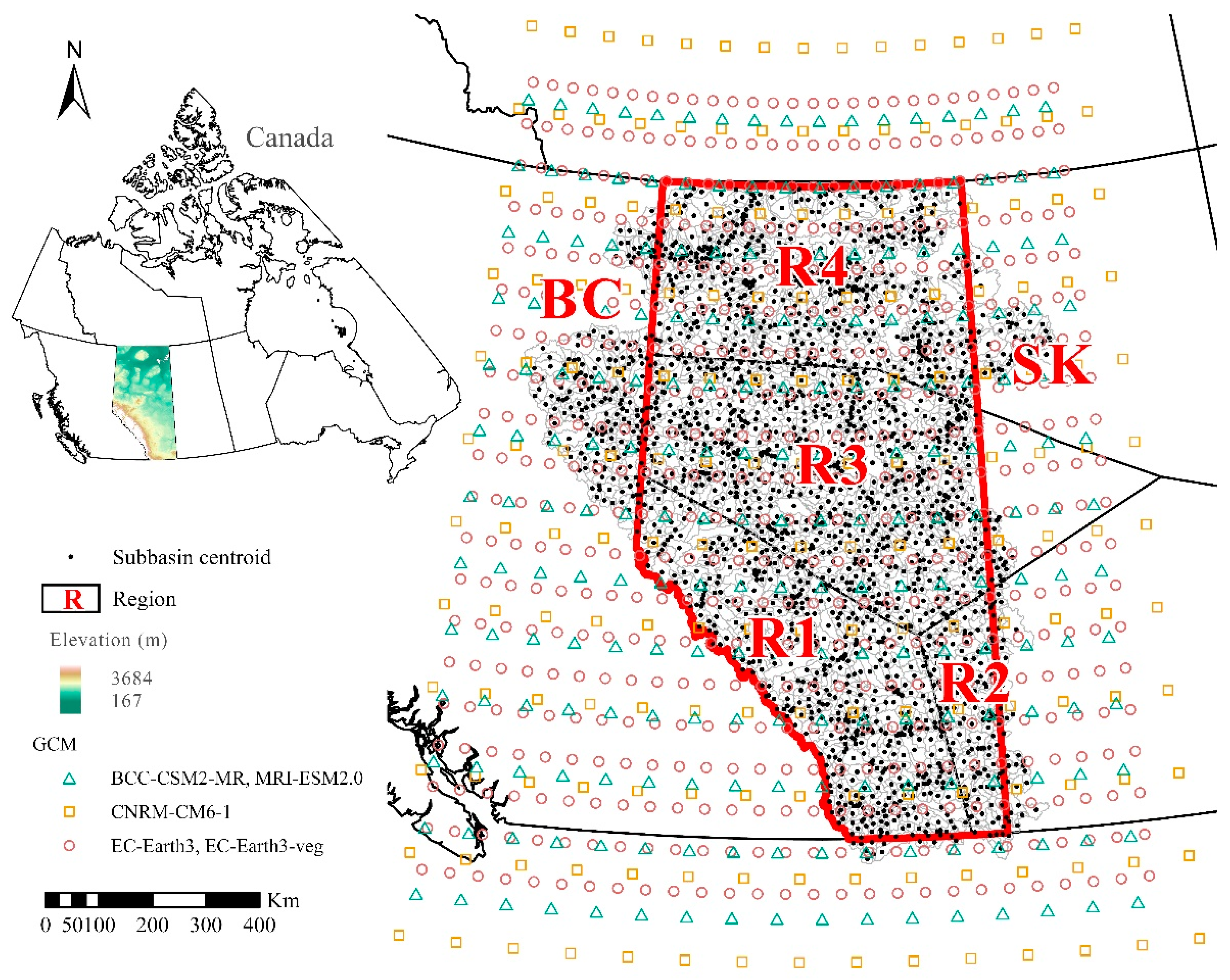
2.1. Study Area

Alberta extends for ~1200 km from north to south (49° N–60° N) and ~660 km (110° W–120° W) across the greatest width with an area spanning 661,000 km². Elevation ranges from 152 m in the northeast to 3747 m in the Rocky Mountains along the south-western border Figure 1. The province has more than one-third of its total area as agricultural land in the south, with a landscape varying from glacial mountain lakes, rolling foothills, and grassland in the south to vast boreal forests in the north [48]. It has a highly variable climate with mean annual precipitation ranging from ~280 mm in the south to ~1000 mm at the higher elevations of the Rocky Mountains with the provincial average of ~500 mm [25]. Mean winter temperatures usually range from −25.1 °C to −9.6 °C, while mean summer temperatures vary between 8.7 °C and 18.5 °C, with the mean annual temperature ranging from 3.6 °C to 4.4 °C [48].

In this study, we evaluated GCMs’ performances across four contiguous homogeneous regions (R1, R2, R3, and R4) of Alberta. These selected regions were defined in [49] and were developed using soft fuzzy clustering algorithms [50]. The regions were validated through a statistical homogeneity test from Hosking Wallis [51] using daily precipitation and multi-hour precipitation extremes data from Environment and Climate Change Canada [49]. Regions outside of the Alberta border include BC (British Columbia, west side) and SK (Saskatchewan, east side) Figure 1.

2.2. Data

We acquired daily precipitation (P), daily minimum (Tmin), and daily maximum temperature (Tmax) outputs from five GCMs (i.e., BCC-CSM2-MR, CNRM-CM6-1, EC-Earth3, EC-Earth3-veg, and MRI-ESM2.0)

Table 1. Description of CMIP6 GCMs selected for the study.

GCM	Host Institute	Resolution	Variant	References
BCC-CSM2-MR	Beijing Climate Center, China Meteorological Administration, China	250 km	r1i1p1f1	[64]
CNRM-CM6-1	Centre National de Recherches Météorologiques (CNRM), France	100 km	r1i1p1f2	[65]
EC-Earth3	European Earth System Model 27 research institutes from 10 European countries	100 km	r4i1p1f1	http://www.ec-earth.org/ *
EC-Earth3-veg	European Earth System Model 27 research institutes from 10 European countries	100 km	r1i1p1f1	http://www.ec-earth.org/ *
MRI-ESM2.0	Meteorological Research Institute (MRI), Japan	100 km	r1i1p1f1	[66]

* Accessed on 15 November 2019.

from the CMIP6 “historical” experiments. The GCMs were selected based on the availability of daily outputs as of December 2019. The historical experiment includes data from 1850–2014.

A reliable observed climate dataset with high spatio-temporal coverage is key to successfully evaluate any newly released climate datasets [52]. In this study, a unique ‘hybrid’ observational dataset was used as the comparison benchmark. It was produced by Faramarzi et al. [53] who employed five climate data sources, including station-based (https://climate.weather.gc.ca/; accessed on 28 June 2014) and gridded products (National Centers for Environmental Prediction’s Climate Forecast System Reanalysis-CFSR, Climate Research Unit Time Series-CRU TS2, CRU TS3.21, and Natural Resources Canada-NRCan) to reproduce observed streamflow records of 130 hydrometric gauging stations across Alberta, Canada. However, in their study, none of the individual datasets showed the best performance as input to determine streamflow. Therefore, following a ‘combination approach’, they came up with a ‘hybrid dataset’ that was used to force a hydrological model from1983–2014 that resulted in a climate data set of 2255 sub-basins covering entire Alberta (Figure 1). The hybrid climate dataset provides daily precipitation, minimum and maximum temperature. The spatial variation of these climate variables was tested and found to be similar to the Alberta Environment and Parks reported climate data [54]. These data have been successfully incorporated in many applications, including flood frequency analysis [16], crop yield simulations [55,56,57], surface and subsurface water interactions [58], and storage changes in wetlands [59]. In this study we employed this hybrid climate dataset (hereafter referred to as observations dataset) as an observed climate dataset for the GCM evaluations.

Due to the different grid projections of the CMIP6 GCMs (Table 1, Figure 1) and to be consistent with hybrid observation datasets at 2255 sub-basins, a reference grid with a horizontal resolution of ~6km following Werner et al. [60] was used. This resulted in a reference grid of 242 longitudes × 181 latitudes covering the entire province (48° N to 60° N and 123° W to 107° W). All model simulated data were interpolated to this grid using thin-plate spline interpolation algorithm [61] before performing any analysis. Thin-plate spline is not scale-invariant because three covariates (latitude, longitude and a climate normal) appear in a nonlinear way in the interpolation and it has been successfully applied to other studies in the northwestern North America [62] and Canada [63]. Taking the centroid of each sub-basin as the station location of the hybrid climate dataset, we applied the nearest neighbor algorithm in the ArcGIS to locate the closest grid point of GCMs to the centroid of sub-basin for the evaluation purposes.

3. Methods

A concise overview of the methods adopted for this study is illustrated in Figure 2, while a detailed description of various components is provided below.

3.1. Evaluation of Mean Climate Characteristics

Mean characteristics (i.e., mean annual precipitation and temperature) of daily climate derived from GCM simulations are compared to corresponding observed characteristics to assess performance errors. The metrics chosen to evaluate Tmax and Tmin were as follows [67].

Slope of the Regression Line times the Coefficient of Determination (bR²)

$$b{R}^2=\left\{\left|b\right|.R^2 if b\le 1; {\left|b\right|}^{-1}{R}^2 if b>1\right\}$$

(1)

where R² is the coefficient of determination between the observed and simulated values, and b is the slope of the regression line [53,68]. The range of R² (0–1) describes how much of the observed dispersion is explained by the model prediction and a model can have good R² value (close to 1) but still over or under prediction. Therefore, the gradient b provides additional information and is weighting the R² values to reflect the model results in a more comprehensive way [68].

Nash-Sutcliffe Efficiency (NSE)

$$NSE=1-\frac{{{\displaystyle \sum }}_{i=1}^N{\left(S_i-O_i\right)}^2}{{{\displaystyle \sum }}_{i=1}^N{\left(O_i-\overline{O}\right)}^2}$$

(2)

where O_i and S_i are the ith observed and simulated variable, respectively. $\overline{O}$ is the mean of observed data for the variable being estimated and N is the total number of observations. NSE is a normalized statistic that determines the relative magnitude of the residual variance (‘noise’) compared to the observed variance (‘information’) [69,70]. NSE values range from −∞ to 1, with NSE = 1 being a match between observed and simulated variable. Any NSE value greater or equal to zero indicates that the simulated value estimated the constituent of concern better than the mean observed value. Similar quantitative statistical metrics have been used in the literature to evaluate GCMs performance in simulating hydro-meteorological variables [71,72,73].

The two sample Kolmogorov–Smirnov (KS) test [74] was incorporated to assess how well the distribution of GCMs simulated daily precipitation matched the observations. The KS test is a nonparametric test of the equality of continuous one-dimensional probability distributions and the KS test statistic (D) quantifies the distance between empirical distribution functions of two samples. The closer this D is to zero, the more likely the two samples are drawn from the same distribution. In this study, the null hypothesis, two samples are drawn from identical population, is examined with the 99% level of confidence. The performance metrics for temperature and KS test for precipitation were applied on each of the selected grids in the study area.

3.2. Evaluation of Extreme Characteristics

Precipitation and temperature extremes are defined as independent daily events exceeding an extreme threshold. We use the peak over threshold (POT) approach to sample independent events from each individual time series such that it provides a comprehensive description of extreme events by retaining both the magnitude and the timing of each event [31,75]. Independent events are then used to fit a Generalized Pareto Distribution (GPD) to analyze the probability of extreme events. However, selecting the optimum threshold that allows retention of the largest sample of excesses above the threshold and assures their independence are two of the major challenges against employing the POT approach [76,77]. At least 1.65 peaks per year are recommended to be selected by the POT method [78].

Defining the threshold value above which peaks are sampled from a data series is not trivial. The success of fitting a probability distribution on the peaks is primarily dependent on the compromise between the variance and the bias-too large a threshold will include very few values to model the tail of the distribution correctly (large variance due to only very extreme observations), whereas too low a threshold will result in selecting non-extreme values and a high bias in the analysis [77]. Here, we employed the Likelihood Ratio Test (LRT) to select the optimum threshold as it has shown to outperform other methods [79]. We employed an algorithm developed in R [80], a language and environment for statistical computing, to automate the LRT threshold selection method following the procedure outlined by Beirlant et al. [81] and Zoglat et al. [79]. In the LRT approach, let u_i and u_k (u_i < u_k) be two threshold candidates and X_ui (X_uk) the vector of observations exceeding u_i (u_k). When u_i an acceptable threshold, u_k is also acceptable. The test accepts the lowest one when two thresholds are admissible. It is worth noting that while graphical methods are good candidates for the choice of threshold, they become unmanageable when the number of time series is large, and they depend on visual investigations that are highly subjective [16]. In this study, the initial u_i was chosen as the 90th percentile (P90) for the dataset under consideration.

Furthermore, to ensure that the extracted peaks are independent, a careful declustering was carried out. A few statistical tools have been developed to filter clustered realizations to yield datasets of independent events, including the most widely-adopted method, ‘declustering’ [31]. The extremal index is chosen to ensure the independence of exceedances [82,83]. Ideally, an extremal index of 1 indicates perfectly independent data while 0 indicates clustered data. The R package ‘POT’ was used for declustering and estimating the extremal index [84].

Three extreme indices, namely consecutive wet days (CWD), summer days (SD), and warm nights (WN), were defined based on the extracted peaks over the threshold

Table 2. Definitions of the extreme indices.

Sl Number	Index	Definition
1	Consecutive wet days (CWD)	Days with daily precipitation greater than the threshold *
2	Summer days (SD)	Days with daily maximum temperature greater than the threshold
3	Warm nights (WN)	Days with daily minimum temperature greater than the threshold

* Initially the threshold is chosen as P90.

. For each index, the duration and frequency were calculated separately. Duration is defined as the continuous sequence of days where the value of the climate variable (precipitation or temperature) exceeded the selected threshold before declustering. At each grid point, the durations of all extreme events over the entire period are averaged to represent one value. Frequency is determined by counting the total number of independent events over the entire period for each grid point.

The behaviour of precipitation and temperature extremes in these data products is described by modeling the tails of their fitted distribution. The evaluation of the heaviness of the tails is done by comparing the tail index (i.e., the shape parameter) of the fitted Generalized Pareto Distribution (GPD) distribution, which governs the magnitude and frequency of extreme events. A light-tailed distribution generates less frequent and milder extremes compared to a heavy-tailed distribution. The tail index was therefore calculated and compared between observations and GCM simulations in order to evaluate the performance of CMIP6 models in capturing the precipitation and temperature extremes. To identify the tail behaviour of extremes, the Generalized Pareto Distribution (GPD) was adopted to model the independent and identically distributed (IID) excesses over an optimum threshold u. The cumulative distribution function (CDF) for the GPD is [85]:

$$G\left(x\right)=\mathrm{Pr}\left(X-u<x|X>u\right)=\{\begin{array}{cc}1-{\left(1+\frac{\xi \left(x-u\right)}{\sigma }\right)}^{-\frac{1}{\xi }},& \xi \ne 0\\ 1-e^{\left(-\frac{x-u}{\sigma }\right)},& \xi =0\end{array}$$

(3)

where x, is the extreme climate variables (in mm for precipitation and °C for temperature), u is the location parameter, σ is the scale parameter, and ξ is the shape parameter. The shape parameter (tail index) determines the qualitative behaviour of the GPD, where a ξ = 0 refers to the exponential distribution, for ξ > 0 the corresponding distribution has a heavy upper tail that behaves like a power function with exponent −1/ξ and for ξ = 1 the distribution is uniform. Having determined the optimum threshold, the parameters of the GPD were estimated using the Maximum Likelihood Estimator (MLE) [86].

3.3. GCM Downscaling

Statistical downscaling provides an efficient and effective means of producing reliable climate variables from a large ensemble of GCMs [60,87]. The ‘ClimDown’ R package [88] was used to downscale the GCM outputs to the specified spatial resolution. The package uses multiple techniques including Climate Imprint (CI) [89,90], Quantile Delta Mapping (QDM) [91], Constructed Analogues (CA) [92], and Bias Correction/Constructed Analogues with Quantile mapping reordering (BCCAQ) [60].

Climate Imprint (CI) works together with Quantile Delta Mapping (QDM). It starts by calculating daily climate anomalies for the GCM dataset at the observation dataset’s period. These daily GCM anomalies are interpolated to the observation dataset’s grid and constitute the ‘CI’. The high-resolution gridded observations are then grouped into months and a climatology is calculated for each month. The observed climatology is then added to the GCM-based CI. The QDM was performed on a point-by-point basis in the finer grid system. It uses the observations and the CI result as input and performs a quantile perturbation/quantile mapping bias correction. CA works independently by spatially aggregating the high-resolution gridded observation dataset up to the GCM scale and then proceeds to bias correct the GCM based on those observations. Then, it searches for the top 30 closest time steps in the gridded observations and makes an “analogue” [92]. This method can also generate estimates of extreme events during downscaling.

The ClimDown package uses an overall algorithm called BCCAQ to combine the results from CI-QDM and CA [60,91]. It reorders data for each fine-scale grid point within a month effectively breaking the overly smooth representation of sub-grid-scale spatial variability inherited from CI-QDM, thereby resulting in a more accurate representation of event-scale spatial gradients. This also prevents the downscaled outputs from drifting too far from the climate model’s long-term trend.

4. Results and Discussion

To ensure that the P, Tmax, and Tmin extremes are IID, the excesses have been declustered. We monitored the extremal index for each sub-basins and confirmed the assumption of independence for both the precipitation and temperature peaks time series.

Table 3. The number of peaks for the daily P, Tmax, and Tmin extremes from observed and GCM simulated data before and after declustering for the period of 1983–2014.

Time Series	P		Tmax		Tmin
	Number of Peaks		Number of Peaks		Number of Peaks
	Before	After	Before	After	Before	After
Observed	361	266	821	285	567	241
BCC-CSM2-MR	957	641	815	222	515	207
CNRM-CM6-1	736	467	811	189	553	205
EC-Earth3	823	519	813	206	535	200
EC-Earth3-veg	820	521	800	203	530	203
MRI-ESM2.0	927	574	896	247	600	217

shows the total number of excesses for the study area and the number of peaks confirmed the assumption that excesses should be a minimum of 1.65 multiplied by the number of years.

4.1. Evaluation of Precipitation Mean Characteristics

Figure 3 shows the spatial distribution of relative difference (percentage change from observations) of mean annual precipitation for five GCMs. The BCC-CSM2-MR, EC-Earth3, and EC-Earth3-veg underestimate the mean annual precipitation in central to northern Alberta and overestimate in southern Alberta. The MRI-ESM2 also overestimates in the southern Alberta while showing a varied pattern in central to northern Alberta. The CNRM-CM6-1 greatly underestimates precipitation for the entire study area except in the Canadian Rockies. The behaviour of all GCMs is fairly similar to simulated precipitation in the mountainous region (south-western), where all models highly overestimate. The spatial pattern and magnitude of observed precipitation shows that this region receives high amounts of precipitation compared to other regions of the province Figure 3. However, the orographic effect and limited number of observation stations in the complex terrain of the Canadian Rockies may play an important role to such big difference. Wong et al. [93] compared several gridded precipitation products over Canada and found that precipitation amounts are overestimated in the Canadian Rockies. Li et al. [94] and Kuo et al. [95] found similar precipitation biases over the Canadian Rockies as simulated by the Weather Research and Forecasting model (WRF).

The KS statistic (D) in Figure 4 supports our findings in Figure 3. Minimum D values are found in northern Alberta followed by central and southern Alberta for all models except the CNRM-CM6-1, which shows large D values across the province. Overall, GCMs have comparatively larger D in the Canadian Rockies. Based on multiple statistical metrics, Cheng et al. [71] also found poor performance of CMIP5 GCMs over the Canadian Rockies portion of the Athabasca River Basin in Alberta. The MRI-ESM2.0 has higher D values in southern Alberta where the magnitudes of overestimation are also higher Figure 3. The KS test for mean annual precipitation shows no statistically significant results for BCC-CSM2-MR, CNRM-CM6-1 and MRI-ESM2.0 for all 2255 sub-basins. The EC-Earth3 and EC-Earth3-veg produce significant results only for two and seven sub-basins, respectively. For evaluating precipitation time series, the number of significant results is in line with expectation, if we assume that precipitation values are spatially and temporally independent [96].

4.2. Evaluation of Maximum and Minimum Temperature Mean Characteristics

The observed average annual Tmax and Tmin and their differences (simulation minus observation) corresponding to five GCMs are presented in Figure 3 for the period 1983–2014. The spatial pattern of biases is somewhat similar for all GCMs. The change is larger ± 5 °C in the south and south-western domain for all GCMs except the MRI-ESM2.0, which also shows overestimation (warm bias) in the central to the northern part of the province. In the BC part, all GCMs underestimate (cold bias) Tmax and Tmin. In the mountainous regions, every GCM overestimate both variables. Overall, most of the models underestimate temperature in southern Alberta and overestimate in the north. Similar temperature biases were reported over the complex topographic regions in other studies [95,97]. Sillmann et al. [37] also reported such limitations in high terrain regions while evaluating climate extremes indices in a CMIP5 multi-model ensemble. This bias could be partly attributed to the poor representation of complex topographic features and the land surface interactions in the parameterization scheme of the GCM [95]. The primary horizontal resolutions between models could introduce large differences in elevation of mountainous terrains, which can make the reproduction of precipitation and temperature difficult [94]. The overestimation of temperature in the mountainous regions might also be attributed to the absence of altitude effects in the interpolation algorithm (Section 2.2) as the temperature varies with elevation [98].

The spatial evaluation metrics of mean annual daily temperature for the five GCMs are presented in Figure 4. The GCMs usually obtain higher skill scores for Tmax compared to Tmin. Similar results were found in a study by Cheng et al. [71], where they evaluated the performance of six CMIP5 GCMs over the Athabasca River Basin in Alberta. Figure 4 reveals a mostly north–south gradient for Tmax and Tmin. Results based on bR² and NSE show clear spatial patterns of improved simulation in the northern area of the province followed by middle, southern and south-western parts. The low bR² and negative NSE values in the south-western region (mountainous) of the province reflect the poor model performance. The bR² ranges from 0.19 to 0.70 and 0.09 to 0.69 for Tmax and Tmin, respectively. Likewise, the NSE metric tends to show a similar pattern as bR² with values ranging from −0.52 to 0.70 and −0.91 to 0.67 for Tmax and Tmin, respectively. Overall, the CNRM-CM6-1, EC-Earth3, and EC-Earth3-veg models perform better in simulating temperature compared to MRI-ESM2.0 and BCC-CSM2-MR. Wyser et al. [39] discussed the impact of forcing datasets (e.g., greenhouse gas concentrations, insolation, stratospheric ozone concentrations, optical properties of stratospheric aerosols, and landuse changes) for climate model simulations and pointed GHG concentrations as a major contributor to the warming. The variation in results from GCMs is probably strongly model-dependent due to variations in considering these forcing datasets.

4.3. Evaluation of Precipitation Extreme Characteristics

The GCM simulations are also evaluated in terms of reproducing the observed duration and frequency of CWD. The duration based on observed data Figure 5 ranges from one to two days and the spatial distribution is uniform over the study area, with a few exceptions in the southern areas where the durations are longer. GCMs reproduce the duration of CWD very well. All GCMs slightly overestimate the duration with a maximum one day except for the BCC-CSM2-MR, which underestimate the duration in most sub-basins (Figure 5).

The mean annual frequencies of CWD compared with observed data are maximum in the northern area followed by the central and southern areas of the province Figure 5. The results show that the frequency estimated from the different GCMs is in good agreement with the observations, except that the BCC-CSM2-MR model overestimates the frequency in most of the sub-basins. The overestimation could be attributed to two aspects of insufficient resolution in the model including a) the resolution is too coarse to represent the landmass at all and b) the model does not resolve the topographically driven high precipitation regimes [99]. For most GCMs, the maximum underestimation of occurrence frequency is found in the south-western mountainous areas, and this underestimation could also be related to the improper representation of uneven topography in the climate model as explained previously.

The temporal distribution of the duration and frequency of CWD are plotted in Figure 6 through kernel density plots that display the distribution of these two characteristics over a continuous interval or time period for the entire province. The peaks of the plot indicate where values are concentrated over the interval. Results are similar to the spatial plots where all models partially coincide at the base of the kernel density curves for the duration and differ slightly at the peaks except for the BCC-CSM2-MR, which agrees at the base but underestimates the peak Figure 6. Likewise, the frequency Figure 6 shows that the graphical patterns of individual models are opposite compared to the pattern for the duration.

4.4. Evaluation of Maximum and Minimum Temperature Extremes Characteristics

The maximum duration (three to four days) of SD and WN is observed in the northernmost and south-western mountainous parts of the province Figure 5. However, the duration of SD progressively decrease from the mountainous area to the grassland region of southern Alberta. The duration of WN is as high as three days in the south-eastern region of Alberta. In rest of the province, the duration ranges from two to three days for both SD and WN. The provincial average duration of SD and WN are 2.7 and 2.5 days, respectively. In Figure 5, the difference of duration indicates that GCMs have a relatively low skill (overestimation) in reproducing the mean duration of SD. The results show that individual model performance varies substantially. The CNRM-CM6-1 model shows very poor performance while the MR-ESM2.0 is comparatively better compared to any other models. Only the MR-ESM2.0 model shows an underestimation of the mean duration of SD in the mountainous region. However, GCMs show better skill in reproducing the mean duration of WN across the province. The BCC-CSM2-MR, CNRM-CM6-1, and MRI-ESM2.0 underestimate mean duration in the Rockies. Overall, the variation in the estimation of the mean duration of WN is within ± 1 day.

We find an inverse relationship between duration and frequency of SD and WN. A sub-basin with a high duration of SD and WN has a low frequency of SD and WN and vice-versa. The spatial pattern of the frequency distribution of SD and WN are also similar to that of mean duration. Results in Figure 5 reveal the minimum frequency of SD and WN in the northern and mountainous regions of the province. Overall, the average number of SD and WN is 13 and 14 across the province, respectively. Based on the overall results, the underestimation of delta mean frequency ranges from 3 to 4 and 0.5 to 1.6, respectively for SD and WN. Nie et al. [44] pointed out the new cloud-fraction scheme updated in the CMIP6 version that might help to improve the simulation of temperature extremes by giving surface radiant fluxes in the low- and mid-latitudes. In their study, they found that the BCC-CSM2-MR model can simulate the warm and cold temperature extremes reasonably well.

Density curves of duration and frequency of SD and WN are shown in Figure 6. The GCM simulated distributions of SD are highly deviated from the observed distributions. All GCMs overestimate the duration and underestimate their frequency. For both characteristics, individual models’ distributions are substantially different from each other. However, duration and frequency distribution curves of WN are similar to the observed distribution. GCMs can partially reproduce the density curves although they overestimate duration and underestimate the frequency of WN.

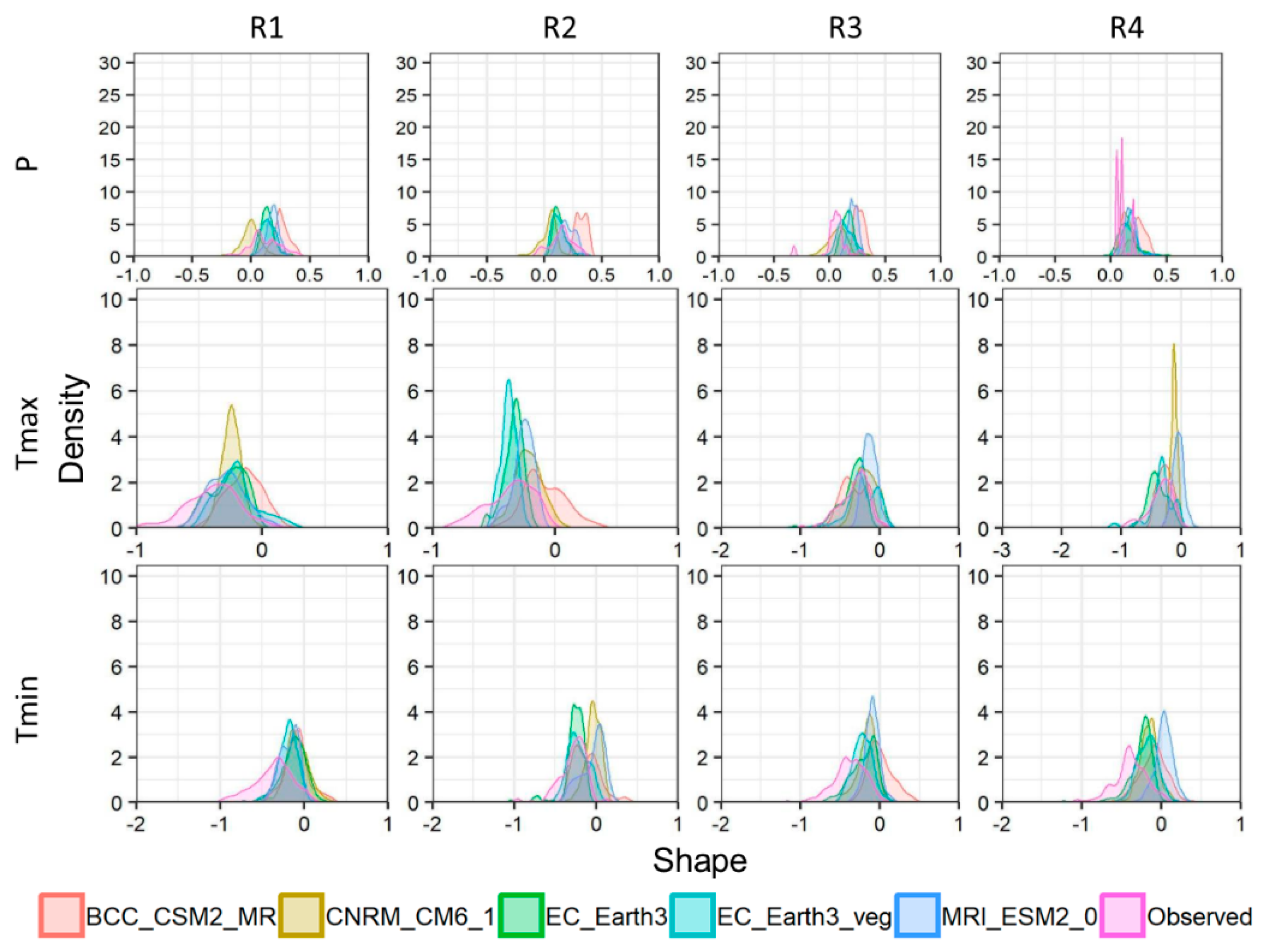
4.5. Tail Behaviour of Precipitation and Temperature Extremes

The tail behaviour of P, Tmax, and Tmin extremes is shown in Figure 7. The observed tail index of P extremes is mostly positive across the province, indicating a heavy-tailed distribution. Results reveal high values of tail index in the southern part of Alberta and BC portion of the study area. The north-eastern part of the province showed thin tails. All GCMs reveal similar spatial patterns of difference, whether over- or underestimation of the tail index for the precipitation extremes with values ranging around ± 0.25, as illustrated in Figure 6. GCMs highly overestimate the tail index. Such over- or underestimation of tail behaviour is also found for CMIP5-GCMs over the Euro-Mediterranean region [100]. The tail behaviour is known to be sensitive to the convective parameterization (CP) within GCMs, which aims to represent the effects of convection on the grid-scale but does not capture the dynamics of individual storms [101]. However, the CP is a major source of errors in climate simulations [94] and therefore, the bias in the tail index estimation is inherent to the climate model performances.

The observed tail index of both Tmax and Tmin extremes are negative for most of the sub-basins, indicating a short-tailed distribution Figure 7. The spatial distribution of tail index is somewhat different for both temperature extremes. Positive values of Tmax extremes are located in the south and north-eastern part of the study area. In addition to these locations, the tail index of Tmin extremes is positive in the foothills of the Rockies. Otherwise, a relatively thin tail (negative) is observed in the entire province. A thin-tailed probability distribution corresponds to the upper tail declining to zero exponentially or faster [102]. GCM simulations are quite biased in reproducing the tail behaviour of extremes. For Tmax extremes, models overestimate in the mountainous area and northernmost Alberta. In terms of bias estimation, the spatial distribution of tail index of Tmax extremes is analogous to the CNRM-CM6-1 and MR-ESM2. For the Tmin extremes, a comparable spatial pattern existed for the delta tail index for all GCMs. Similar to the results of Tmax extremes, the magnitude of bias (overestimation) based on Tmin extremes is higher for most of the sub-basins.

The temporal distribution of density curves of the tail index for P extremes Figure 8 shows that all GCMs slightly overestimate the index with comparable height except the CNRM-CM6-1, which has similar base as the observations with a short peak. For Tmax extremes, GCMs reproduce the tail index very well at the base; however, they overestimate the peak, which is higher than the observed tail index (Figure 8). GCMs show biases (overestimation) both at the base and peak for the Tmin extremes (Figure 8) and their temporal distributions are similar. The three-parameter distributions (e.g., GPD) are less parsimonious than the two-parameter distributions and have large parametric uncertainty in estimating the tail index. However, there are ways (e.g., regionalization) to improve the accuracy of this parameter estimation by maintaining spatial homogeneity [49]. Regionalization increases the robustness in estimation by increasing the sample size by substituting space for time [51], which can be followed in future studies.

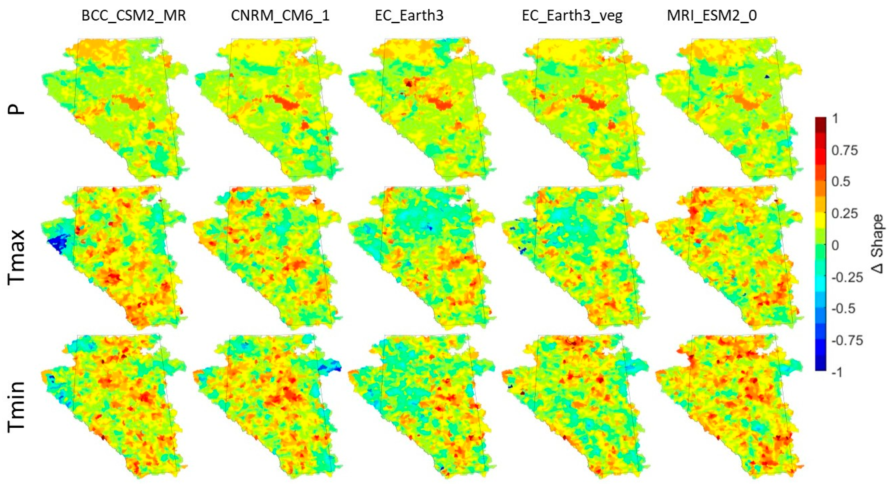
4.6. Regional Variation of GCM Performances

In this section, we discuss GCMs’ performances in reproducing the extremes of P, Tmax, and Tmin in the four identified regions within Alberta Figure 1.

4.6.1. Extreme Characteristics

The regional distributions of density curves (Figure 9) show fluctuation in densities of mean duration and frequency of CWD, SD, and WN. The shape of the distribution varies across regions. The western mountainous region (R1) has flat shaped density curves with reduced peaks for both duration and frequency. R2, which consists of grassland with low annual precipitation and high temperature [103], has the highest peak for both duration and frequency. Different components of the biosphere control the regional climate feedback processes that may govern the variability of GCM simulations across regions. Consequently, we observe variation in results across regions as simulated by a single GCM. The inter-model variability in reproducing duration of CWD is less than that of frequency. For SD, all GCM simulations are very different from the observed distribution of duration and frequency of SD. For WN, GCMs slightly overestimate the duration and underestimate the frequency in all regions.

4.6.2. Tail Behaviour of Extremes

The tail behaviour of P extremes in Figure 10 shows that the majority of GCMs produce the tails index quite well in all regions, except the BCC-CSM2-MR which has a slight overestimation. In R4, the observed tail behaviour of P extremes is somewhat complex with multiple peaks, and the behaviour is not reproduced by any GCM. However, the performance of GCMs is better for the Tmax and Tmin extremes where simulated peaks of density curves are higher than that of observed density curve.

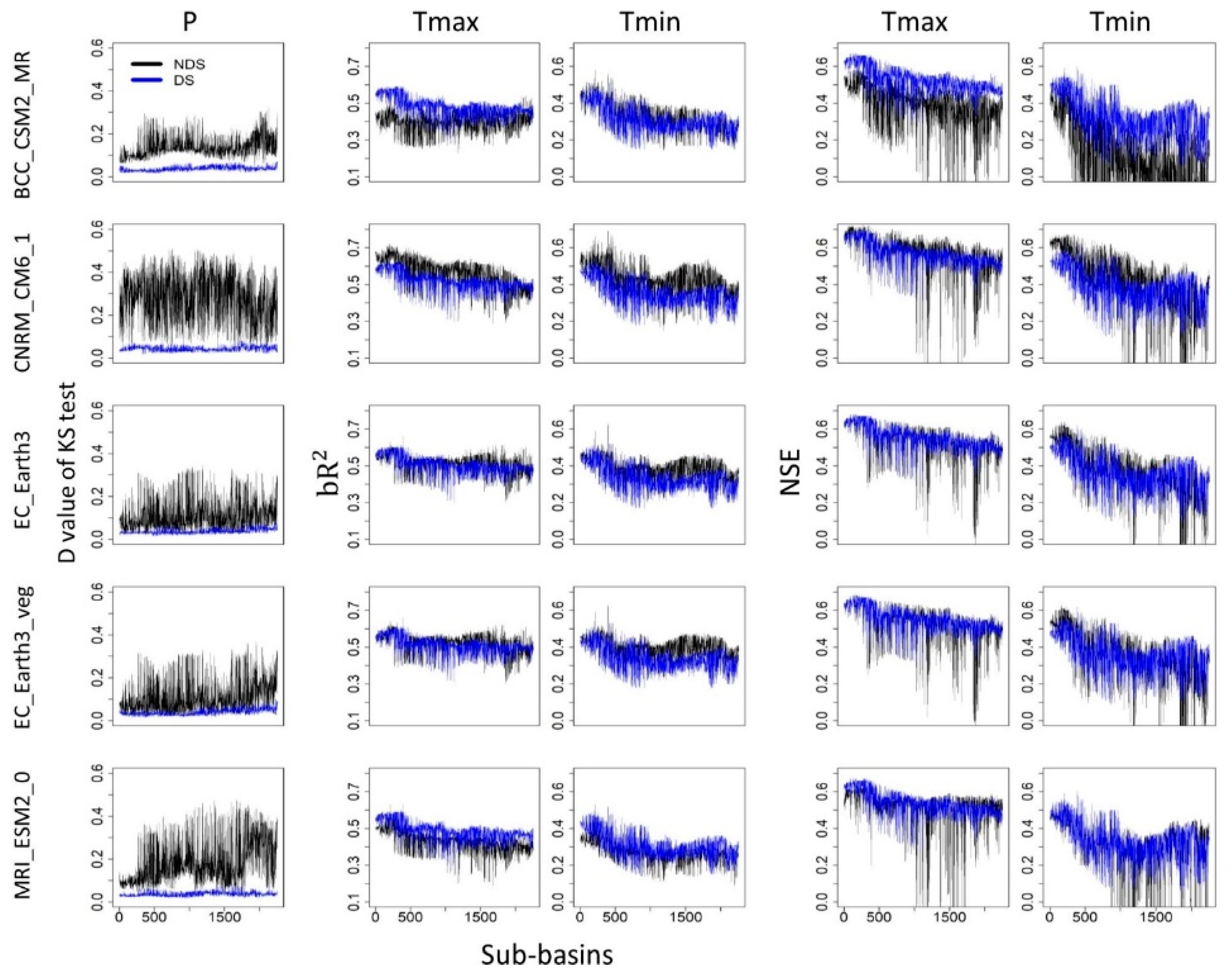
4.7. Evaluation of Mean and Extreme Characteristics of Downscaled Simulations

The KS statistic (D) is calculated using the downscaled (DS) and non-downscaled (NDS) data against the observations (Figure 11). The reduced magnitude of D clearly indicates the overall improved precipitation prediction skills of GCM simulations across the province. The D value is decreased from 0.02–0.50 (NDS) to 0.01–0.11 (DS). NDS GCMs obviously show poor performance (Figure 3) compared with DS GCMs in simulating precipitation. However, in contrast to the precipitation, bias correction and downscaling the temperature ensemble time series led to a poorer prediction skill for the GCMs (Figure 11). This observation indicates that the GCMs (NDS) that participated in CMIP6 are reasonably good at simulating daily maximum and minimum temperatures. Based on bR² and NSE metrics, the bias correction and downscaling of Tmax only improve BCC-CSM2-MR and MRI-ESM2.0 GCMs prediction skills. The other GCMs either underperform or perform similar to NDS GCMs. For Tmin, only the MRI-ESM2.0 GCM shows better performance after bias correction and downscaling. For the BCC-CSM2-MR GCM, the two metrics (bR² and NSE) show different results for many sub-basins. The other three GCMs (CNRM-CM6-1, EC-Earth3, EC-Earth3-veg) show better skill in their non-downscaled simulations.

The DS GCM simulations are further assessed using three extremes indices (CWD, SD, and WN). We extracted two characteristics (i.e., duration and frequency) of each index using DS simulations and estimated the difference between DS and observations for each sub-basin. The delta duration and frequency of CWD (Figure 12) show the close representation of DS simulations to observations, indicating better skills of DS GCMs. Likewise, the difference of duration and frequency based on SD and WN between the DS GCM simulations and observations is reduced across the province. Similar to the mean characteristics, DS GCMs show better skill in reproducing extreme precipitation characteristics compared with the temperature extremes.

Figure 13 shows the spatial distribution of the delta tail index of P, Tmax, and Tmin extremes for DS GCM simulations. There is no clear indication that DS GCMs perform better than the NDS GCMs (Figure 6). The spatial pattern of the delta tail index shows that the magnitude of differences decrease in most of the sub-basins. There are some opposite signals also found for all extremes, and more specifically, overestimation by DS GCM and underestimation by NDS GCM. For example, the DS CNRM-CM6-1 overestimates (Figure 13) while this GCM underestimates the tail index under NDS condition (Figure 7).

Note that the bias correction and downscaling generally involves processes that bring the climate model simulations close to the observations; however, the bias-corrected and downscaled simulations always carry the climate change signal from the host model [99]. Therefore, results based on DS simulations do not substantially increase the confidence as shown in the Figure 11, Figure 12 and Figure 13. However, results show that the bias correction and downscaling approach reasonably reproduced mean and extremes (especially for precipitation). These results are not surprising as Li et al. [94] and Kuo et al. [95] used dynamical downscaling approach to downscale historical climate over western Canada and found similar results, although dynamical downscaling showed better ability over statistical downscaling [99].

5. Summary and Conclusions

This study analyzed the performance of five CMIP6 GCMs in their ability to simulate the observed spatio-temporal behaviour of climate means and extremes across 2255 sub-basins in Alberta, Canada. Daily simulations of P, Tmax, and Tmin were evaluated against a hybrid observational data set that best represents the climatic and hydroclimatic conditions of the province. Despite similar spatial resolutions, model performances varied in their ability to simulate the means and extremes of precipitation and temperatures. From the various analyses presented and discussed in this study, we summarize and conclude the following main outcomes.

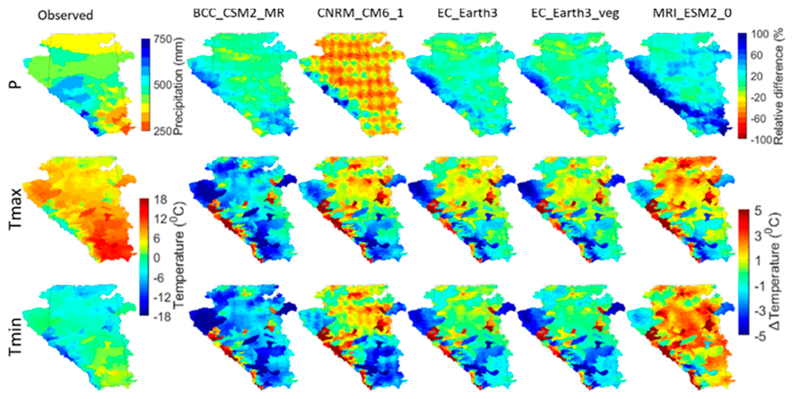
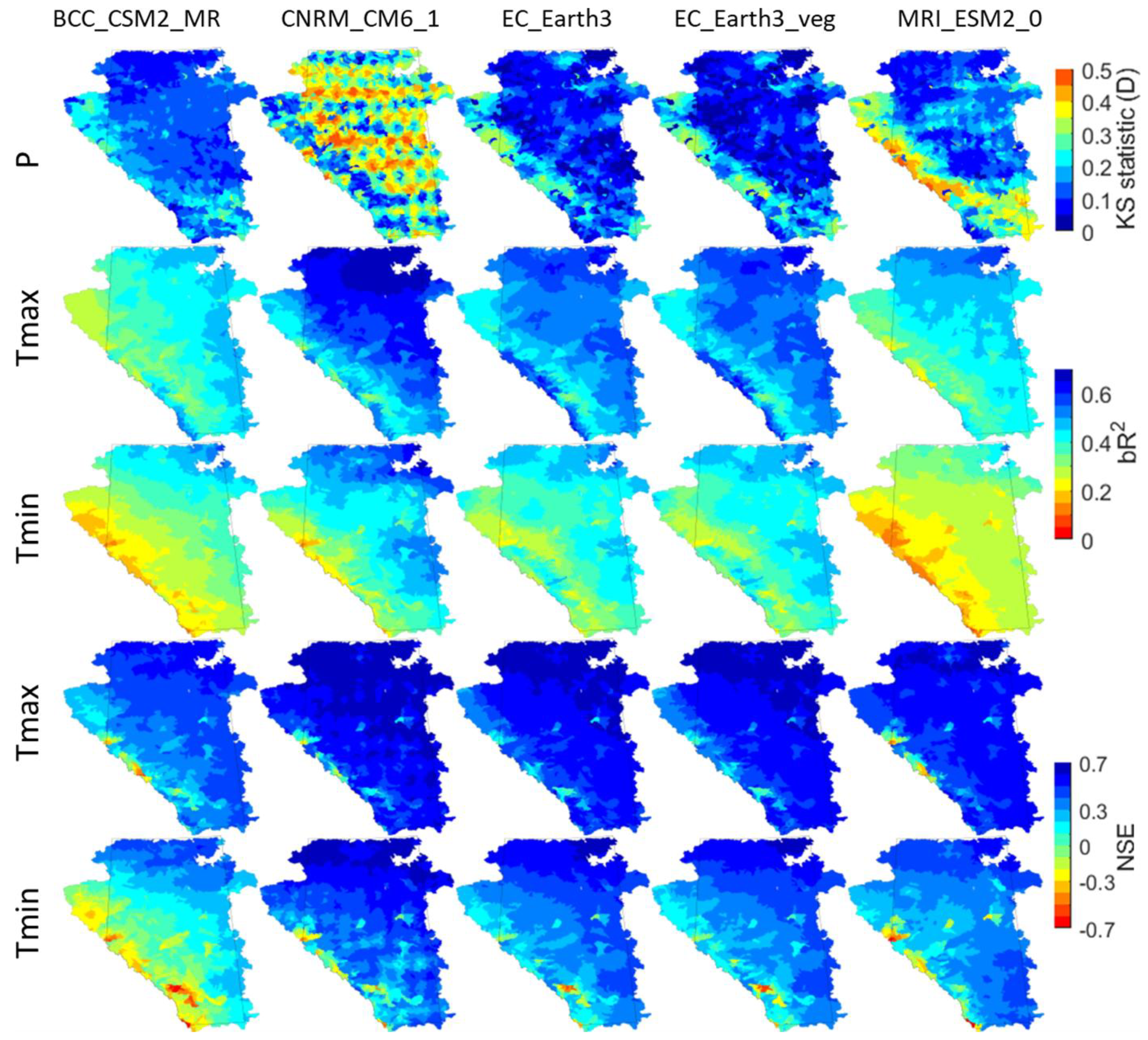
• The average bias in mean annual precipitation is reasonably low for all sub-basins, except for the CNRM-CM6-1 GCM. The EC-Earth3 and EC-Earth3-veg simulate the annual mean P quite well followed by the MRI-ESM2.0 and BCC-CSM2-MR. However, the performance of CNRM-CM6-1 is very poor with substantial underestimation. For temperature, the MRI-ESM2.0 shows the worst performance. The EC-Earth3 and EC-Earth3-veg show better skill followed by the BCC-CSM2-MR and CNRM-CM6-1. Overall, models show better performance in simulating Tmax than Tmin. For both precipitation and temperature, models reproduced the observations better in the north and follow a gradient toward the south with poorest performance in the mountainous area.
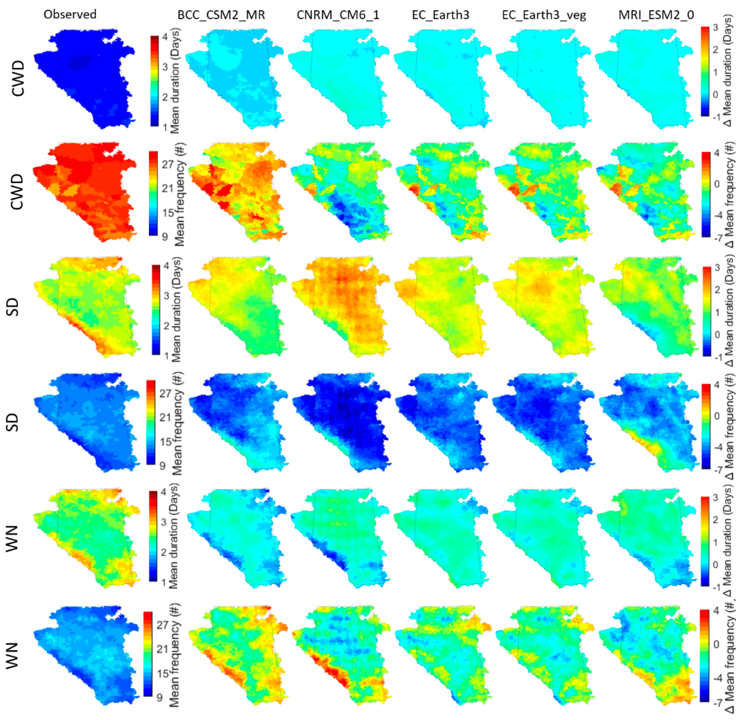
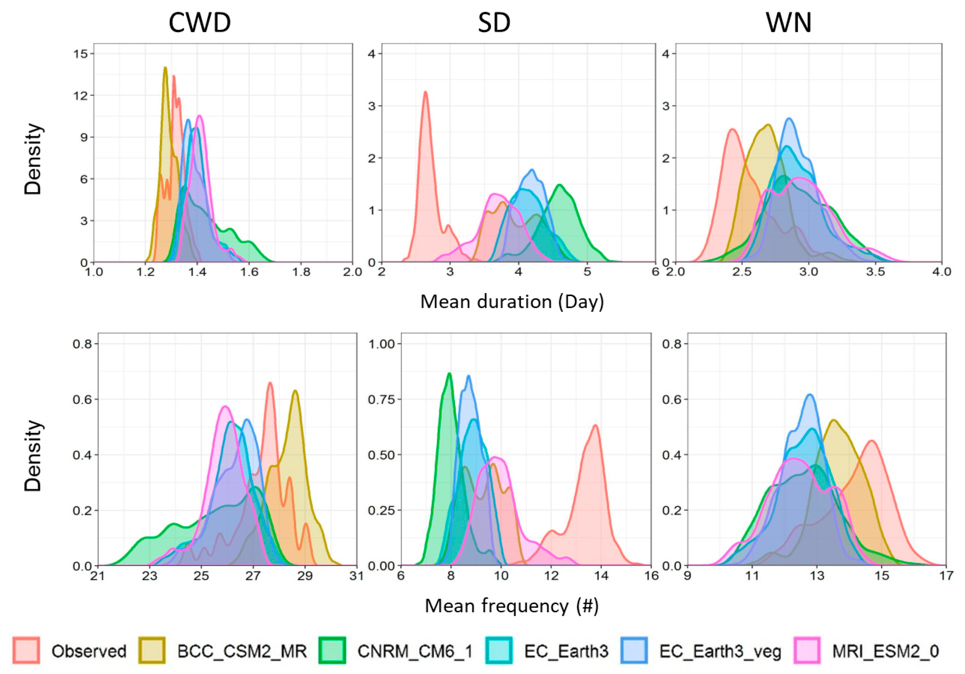
• Minimum positive performance errors (overestimation) are found for the mean annual duration of CWD followed by WN and SD. The BCC-CSM2-MR performed poorly with respect to the duration of CWD, as did the CNRM-CM6-1 regarding the duration of both SD and WN (compared to other GCMs for the entire domain of study). The temporal distributions of duration by model simulations are reasonably superimposed to that of observations in the case of CWD; however, they are slightly and completely overestimated by GCMs for the duration of WN and SD, respectively. In general, there is an inverse relationship between the duration and frequency of occurrence of extreme indices. GCMs consistently underestimated the frequency whereas they overestimated the duration. Nevertheless, the performance of the individual models to simulate frequency is rather similar to that of duration. For all extreme indices, a pattern of over- or underestimating the duration/frequency observed in the southwestern side of the province where the Canadian Rockies are located. Therefore, it would be interesting to investigate the bias–topography relationship during subsequent verification studies across mountainous regions of North America.
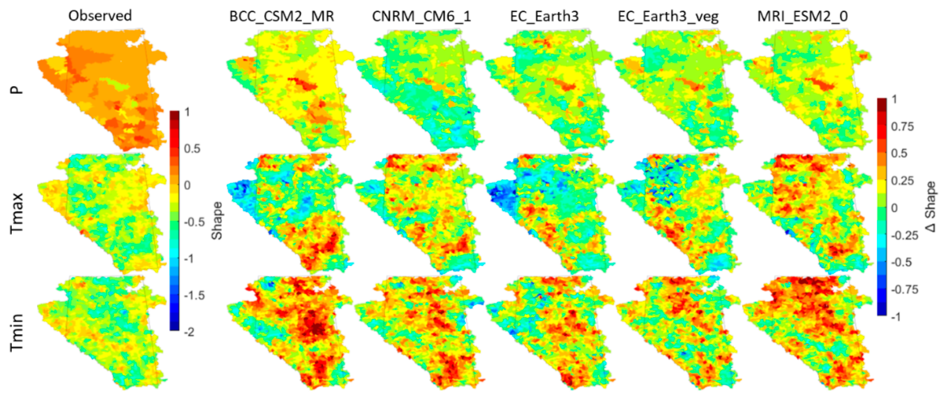
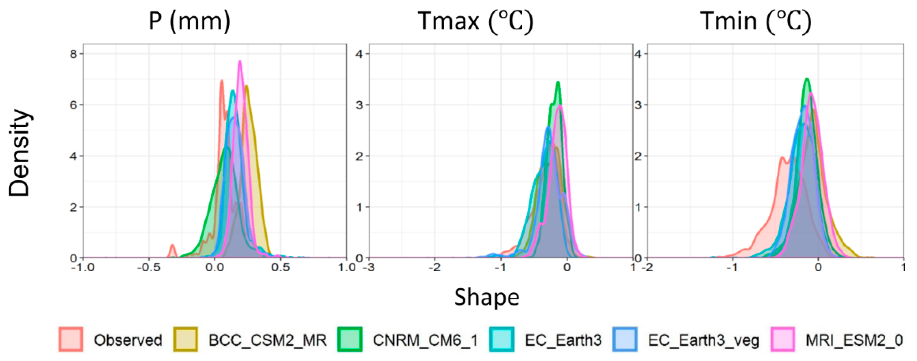
• The observed tail index (shape parameter of the Generalized Pareto Distribution) indicated a heavy tail for P extremes and light tail for Tmax and Tmin extremes. The tail index reasonably follows the spatial distribution of observations. However, a little difference in the tail of distribution significantly affects the long return periods indicating the importance of good tail representation. In this aspect, GCMs still may not incorporate the convective parameterization scheme at the existing grid spacing. The individual model performance is quite similar for all extremes having the poorest performance (highest magnitude of errors) by the BCC-CSM2-MR for P, MRI-ESM2.0 for Tmax, and both BCC-CSM2-MR and MRI-ESM2.0 for Tmin extremes.
• The downscaled GCMs showed better skill in simulating mean annual precipitation compared to the non-downscaled GCMs. The performance of DS GCM simulations was not satisfactory for Tmax and Tmin. The DS technique improved Tmax simulations by the BCC-CSM2-MR and MRI-ESM2.0. Only the MRI-ESM2.0 showed better performances in Tmin after downscaling. However, GCMs showed good skills when reproducing the characteristics (duration and frequency of occurrence) of CWD, SD, and WN based on DS simulations (as compared to NDS simulations). Overall, the bias correction and downscaling approach worked well for reproducing extreme characteristics, and more specifically, improved CWD’s characteristics over those associated with SD and WN. After downscaling, there is no clear indication of having an improved tail index of GPD based on precipitation and temperature extremes. The downscaled simulations do not significantly increase our confidence to simulate climate variables, specifically the Tmax and Tmin time series.

It is obvious that results from each GCM would be different in terms of spatial and temporal scale. The physical reasons behind any over- or underestimation by individual GCMs would require more in-depth and perhaps process-based analyses. We considered the best available hybrid observation dataset to evaluate the performance of five CMIP6 GCMs to simulate the means and extremes of several climatic variables. However, their performances can also be evaluated through using different reanalysis and global and regional gridded climate products to draw more robust conclusions. Poor model performances in the mountainous region may arise due to the lack of high-quality observed data in that region. Several factors affect the GCMs’ performance including the choice and quality of observed hybrid dataset and performance metrics. Application of quantitative statistical metrics (bR² and NSE) may compromise the presence of uncorrelated day-to-day variations, which account for a large portion of total variability. In such cases, validation statistics like distribution of time series and autocorrelation functions, that do not depend on direct correlation between time series, can be applied simultaneously to further check the GCM’s performances in reproducing observed behaviour of climate means and extremes. Despite these limitations and based on our statistical analysis of precipitation and temperature data, our study provides useful information about GCMs performances in simulating means and extremes of daily P, Tmax, and Tmin across Alberta. Such information clearly lays the foundation for future climate impact analysis using CMIP6 GCMs.

References

1. Eyring, V.; Bony, S.; Meehl, G.A.; Senior, C.A.; Stevens, B.; Stouffer, R.J.; Taylor, K.E. Overview of the Coupled Model Intercomparison Project Phase 6 (CMIP6) experimental design and organization. Geosci. Model Dev. 2016, 9, 1937–1958. [Google Scholar] [CrossRef] [Green Version]
2. Taylor, K.E.; Stouffer, R.J.; Meehl, G.A. An overview of CMIP5 and the experiment design. Bull. Am. Meteorol. Soc. 2012, 93, 485–498. [Google Scholar] [CrossRef] [Green Version]
3. Riahi, K.; van Vuuren, D.P.; Kriegler, E.; Edmonds, J.; O’Neill, B.C.; Fujimori, S.; Bauer, N.; Calvin, K.; Dellink, R.; Fricko, O.; et al. The Shared Socioeconomic Pathways and their energy, land use, and greenhouse gas emissions implications: An overview. Glob. Environ. Chang. 2017, 42, 153–168. [Google Scholar] [CrossRef] [Green Version]
4. Van Vuuren, D.P.; Edmonds, J.; Kainuma, M.; Riahi, K.; Thomson, A.; Hibbard, K.; Hurtt, G.C.; Kram, T.; Krey, V.; Lamarque, J.F.; et al. The representative concentration pathways: An overview. Clim. Chang. 2011, 109, 5–31. [Google Scholar] [CrossRef]
5. Stouffer, R.J.; Eyring, V.; Meehl, G.A.; Bony, S.; Senior, C.; Stevens, B.; Taylor, K.E. CMIP5 Scientific Gaps and Recommendations for CMIP6. Bull. Am. Meteorol. Soc. 2017, 98, 95–105. [Google Scholar] [CrossRef]
6. Solomon, S.; Manning, M.; Marquis, M.; Qin, D. IPCC Climate Change 2007: The Physical Science Basis. Contribution of Working Group I to the Fourth Assessment Report of the Intergovernmental Panel on Climate Change; Cambridge University Press: Cambridge, UK, 2007. [Google Scholar]
7. Easterling, D.R.; Kunkel, K.E.; Arnold, J.R.; Knutson, T.; LeGrande, A.N.; Leung, L.R.; Vose, R.S.; Waliser, D.E.; Wehner, M.F. Precipitation Change in the United States. In Climate Science Special Report: Fourth National Climate Assessment, Volume I; Wuebbles, D.J., Fahey, D.W., Hibbard, K.A., Dokken, D.J., Stewart, B.C., Maycock, T.K., Eds.; U.S. Global Change Research Program: Washington, DC, USA, 2017. [Google Scholar]
8. Zhang, X.; Flato, G.; Kirchmeier-Young, M.; Vincent, L.A.; Wan, H.; Wang, X.; Rong, R.; Fyfe, J.C.; Li, G.; Kharin, V.V. Changes in Temperature and Precipitation Across Canada. In Canada’s Changing Climate Report; Chapter 4; Bush, E., Lemmen, D.S., Eds.; Government of Canada: Ottawa, ON, Canada, 2019. [Google Scholar]
9. Roots, E.F. Climate change: High-latitude regions. Clim. Chang. 1989, 15, 223–253. [Google Scholar] [CrossRef]
10. Vose, R.S.; Easterling, D.R.; Kunkel, K.E.; LeGrande, A.N.; Wehner, M.F. Temperature Changes in the United States. In Climate Science Special Report: Fourth National Climate Assessment, Volume I; Wuebbles, D.J., Fahey, D.W., Hibbard, K.A., Dokken, D.J., Stewart, B.C., Maycock, T.K., Eds.; U.S. Global Change Research Program: Washington, DC, USA, 2017. [Google Scholar]
11. Yang, Y.; Bai, L.; Wang, B.; Wu, J.; Fu, S. Reliability of the global climate models during 1961–1999 in arid and semiarid regions of China. Sci. Total Environ. 2019, 667, 271–286. [Google Scholar] [CrossRef] [PubMed]
12. Kharin, V.V.; Flato, G.M.; Zhang, X.; Gillett, N.P.; Zwiers, F.; Anderson, K.J. Risks from climate extremes change differently from 1.5 °C to 2.0 °C depending on rarity. Earth’s Future 2018, 6, 704–715. [Google Scholar] [CrossRef]
13. O’Neill, M.S.; Ebi, K.L. Temperature extremes and health: Impacts of climate variability and change in the United States. J. Occup. Environ. Med. 2009, 51, 13–25. [Google Scholar] [CrossRef] [PubMed]
14. Field, C.B.; Barros, V.; Stocker, T.F.; Dahe, Q. (Eds.) IPCC Managing the Risks of Extreme Events and Disasters to Advance Climate Change Adaptation: Special Report of the Intergovernmental Panel on Climate Change; Cambridge University Press: Cambridge, UK, 2012. [Google Scholar]
15. Reichstein, M.; Bahn, M.; Ciais, P.; Frank, D.; Mahecha, M.D.; Seneviratne, S.I.; Zscheischler, J.; Beer, C.; Buchmann, N.; Frank, D.C.; et al. Climate extremes and the carbon cycle. Nature 2013, 500, 287–295. [Google Scholar] [CrossRef] [PubMed]
16. Ammar, M.E.; Gharib, A.; Islam, Z.; Davies, E.G.R.; Seneka, M.; Faramarzi, M. Future floods using hydroclimatic simulations and peaks over threshold: An alternative to nonstationary analysis inferred from trend tests. Adv. Water Resour. 2020, 136, 103463. [Google Scholar] [CrossRef]
17. Archfield, S.A.; Hirsch, R.M.; Viglione, A.; Blöschl, G. Fragmented patterns of flood change across the United States. Geophys. Res. Lett. 2016, 43, 232–239. [Google Scholar] [CrossRef]
18. Hall, J.; Arheimer, B.; Borga, M.; Brázdil, R.; Claps, P.; Kiss, A.; Kjeldsen, T.R.; Kriauĉuniene, J.; Kundzewicz, Z.W.; Lang, M.; et al. Understanding flood regime changes in Europe: A state-of-the-art assessment. Hydrol. Earth Syst. Sci. 2014, 18, 2735–2772. [Google Scholar] [CrossRef] [Green Version]
19. Hajat, S.; Vardoulakis, S.; Heaviside, C.; Eggen, B. Climate change effects on human health: Projections of temperature-related mortality for the UK during the 2020s, 2050s and 2080s. J. Epidemiol. Community Health 2014, 68, 641–648. [Google Scholar] [CrossRef] [PubMed] [Green Version]
20. Gaupp, F.; Hall, J.; Hochrainer-stigler, S.; Dadson, S. Changing risks of simultaneous global breadbasket failure. Nat. Clim. Chang. 2019, 10, 54–57. [Google Scholar] [CrossRef]
21. Pomeroy, J.W.; Stewart, R.E.; Whitfield, P.H. The 2013 flood event in the South Saskatchewan and Elk River basins: Causes, assessment and damages. Can. Water Resour. J. 2016, 41, 105–117. [Google Scholar] [CrossRef]
22. Milrad, S.M.; Gyakum, J.R.; Atallah, E.H. A Meteorological Analysis of the 2013 Alberta Flood: Antecedent Large-Scale Flow Pattern and Synoptic–Dynamic Characteristics. Mon. Weather Rev. 2015, 143, 2817–2841. [Google Scholar] [CrossRef]
23. Teufel, B.; Diro, G.T.; Whan, K.; Milrad, S.M.; Jeong, D.I.; Ganji, A.; Huziy, O.; Winger, K.; Gyakum, J.R.; de Elia, R.; et al. Investigation of the 2013 Alberta flood from weather and climate perspectives. Clim. Dyn. 2017, 48, 2881–2899. [Google Scholar] [CrossRef] [Green Version]
24. Bonsal, B.R.; Wheaton, E.E.; Chipanshi, A.C.; Lin, C.; Sauchyn, D.J.; Wen, L. Drought Research in Canada: A Review. Atmosphere-Ocean 2011, 49, 303–319. [Google Scholar] [CrossRef]
25. Masud, M.B.; Khaliq, M.N.; Wheater, H.S. Analysis of meteorological droughts for the Saskatchewan River Basin using univariate and bivariate approaches. J. Hydrol. 2015, 522, 452–466. [Google Scholar] [CrossRef]
26. Wheaton, E.; Kulshreshtha, S.; Wittrock, V.; Koshida, G. Dry times: Hard lessons from the Canadian drought of 2001 and 2002. Can. Geogr. Géogr. Can. 2008, 52, 241–262. [Google Scholar] [CrossRef]
27. Wehner, M.F. Very extreme seasonal precipitation in the NARCCAP ensemble: Model performance and projections. Clim. Dyn. 2013, 40, 59–80. [Google Scholar] [CrossRef] [Green Version]
28. Kharin, V.V.; Zwiers, F.W.; Zhang, X.; Hegerl, G.C. Changes in temperature and precipitation extremes in the IPCC ensemble of global coupled model simulations. J. Clim. 2007, 20, 1419–1444. [Google Scholar] [CrossRef] [Green Version]
29. Papalexiou, S.M.; Koutsoyiannis, D.; Makropoulos, C. How extreme is extreme? An assessment of daily rainfall distribution tails. Hydrol. Earth Syst. Sci. 2013, 17, 851–862. [Google Scholar] [CrossRef] [Green Version]
30. Serinaldi, F.; Kilsby, C.G. Rainfall extremes: Toward reconciliation after the battle of distributions. Water Resour. Res. 2014, 50, 336–352. [Google Scholar] [CrossRef] [PubMed] [Green Version]
31. Coles, S. An Introduction to Statistical Modeling of Extreme Values; Springer Series in Statistics; Springer: London, UK, 2001; ISBN 978-1-84996-874-4. [Google Scholar]
32. Loikith, P.C.; Neelin, J.D. Short-tailed temperature distributions over North America and implications for future changes in extremes. Geophys. Res. Lett. 2015, 42, 8577–8585. [Google Scholar] [CrossRef] [Green Version]
33. Karl, T.R.; Nicholls, N.; Ghazi, A. CLIVAR/GCOS/WMO Workshop on Indices and Indicators for Climate Extremes Workshop Summary. In Weather and Climate Extremes; Springer: Dordrecht, The Netherlands, 1999; pp. 3–7. [Google Scholar]
34. Frich, P.; Alexander, L.; Della-Marta, P.; Gleason, B.; Haylock, M.; Klein Tank, A.; Peterson, T. Observed coherent changes in climatic extremes during the second half of the twentieth century. Clim. Res. 2002, 19, 193–212. [Google Scholar] [CrossRef] [Green Version]
35. Donat, M.G.; Alexander, L.V.; Yang, H.; Durre, I.; Vose, R.; Dunn, R.J.H.; Willett, K.M.; Aguilar, E.; Brunet, M.; Caesar, J.; et al. Updated analyses of temperature and precipitation extreme indices since the beginning of the twentieth century: The HadEX2 dataset. J. Geophys. Res. Atmos. 2013, 118, 2098–2118. [Google Scholar] [CrossRef]
36. Zhang, X.; Alexander, L.; Hegerl, G.C.; Jones, P.; Tank, A.K.; Peterson, T.C.; Trewin, B.; Zwiers, F.W. Indices for monitoring changes in extremes based on daily temperature and precipitation data. Wiley Interdiscip. Rev. Clim. Chang. 2011, 2, 851–870. [Google Scholar] [CrossRef]
37. Sillmann, J.; Kharin, V.V.; Zhang, X.; Zwiers, F.W.; Bronaugh, D. Climate extremes indices in the CMIP5 multimodel ensemble: Part 1. Model evaluation in the present climate. J. Geophys. Res. Atmos. 2013, 118, 1716–1733. [Google Scholar] [CrossRef]
38. Sulikowska, A.; Wypych, A. Summer temperature extremes in Europe: How does the definition affect the results? Theor. Appl. Climatol. 2020, 141, 19–30. [Google Scholar] [CrossRef] [Green Version]
39. Wyser, K.; Kjellström, E.; Koenigk, T.; Martins, H.; Döscher, R. Warmer climate projections in EC-Earth3-Veg: The role of changes in the greenhouse gas concentrations from CMIP5 to CMIP6. Environ. Res. Lett. 2020, 15, 054020. [Google Scholar] [CrossRef]
40. Chen, H.; Sun, J.; Lin, W.; Xu, H. Comparison of CMIP6 and CMIP5 models in simulating climate extremes. Sci. Bull. 2020, 65, 10–13. [Google Scholar] [CrossRef]
41. Zhu, J.; Poulsen, C.J.; Otto-Bliesner, B.L. High climate sensitivity in CMIP6 model not supported by paleoclimate. Nat. Clim. Chang. 2020, 10, 378–379. [Google Scholar] [CrossRef]
42. Grose, M.R.; Narsey, S.; Delage, F.P.; Dowdy, A.J.; Bador, M.; Boschat, G.; Chung, C.; Kajtar, J.B.; Rauniyar, S.; Freund, M.B.; et al. Insights From CMIP6 for Australia’s Future Climate. Earth’s Future 2020, 8, e2019EF001469. [Google Scholar] [CrossRef] [Green Version]
43. Xin, X.; Wu, T.; Zhang, J.; Yao, J.; Fang, Y. Comparison of CMIP6 and CMIP5 simulations of precipitation in China and the East Asian summer monsoon. Int. J. Climatol. 2020, 40, 6423–6440. [Google Scholar] [CrossRef] [Green Version]
44. Nie, S.; Fu, S.; Cao, W.; Jia, X. Comparison of monthly air and land surface temperature extremes simulated using CMIP5 and CMIP6 versions of the Beijing Climate Center climate model. Theor. Appl. Climatol. 2020, 140, 487–502. [Google Scholar] [CrossRef]
45. Kim, Y.H.; Min, S.K.; Zhang, X.; Sillmann, J.; Sandstad, M. Evaluation of the CMIP6 multi-model ensemble for climate extreme indices. Weather Clim. Extrem. 2020, 29, 100269. [Google Scholar] [CrossRef]
46. Srivastava, A.; Grotjahn, R.; Ullrich, P.A. Evaluation of historical CMIP6 model simulations of extreme precipitation over contiguous US regions. Weather Clim. Extrem. 2020, 29, 100268. [Google Scholar] [CrossRef]
47. Rivera, J.A.; Arnould, G. Evaluation of the ability of CMIP6 models to simulate precipitation over Southwestern South America: Climatic features and long-term trends (1901–2014). Atmos. Res. 2020, 241, 104953. [Google Scholar] [CrossRef]
48. Jiang, R.; Gan, T.Y.; Xie, J.; Wang, N.; Kuo, C.-C. Historical and potential changes of precipitation and temperature of Alberta subjected to climate change impact: 1900–2100. Theor. Appl. Clim. 2017, 127, 725–739. [Google Scholar] [CrossRef]
49. Masud, M.B.; Khaliq, M.N.; Wheater, H.S. Projected changes to short- and long-duration precipitation extremes over the Canadian Prairie Provinces. Clim. Dyn. 2017, 49, 1597–1616. [Google Scholar] [CrossRef]
50. Asong, Z.E.; Khaliq, M.N.; Wheater, H.S. Regionalization of precipitation characteristics in the Canadian Prairie Provinces using large-scale atmospheric covariates and geophysical attributes. Stoch. Environ. Res. Risk Assess. 2014, 29, 875–892. [Google Scholar] [CrossRef]
51. Hosking, J.R.M.; Wallis, J.R. Regional Frequency Analysis; Cambridge University Press: Cambridge, UK, 1997; ISBN 9780521430456. [Google Scholar]
52. Eum, H.I.; Gupta, A.; Dibike, Y. Effects of univariate and multivariate statistical downscaling methods on climatic and hydrologic indicators for Alberta, Canada. J. Hydrol. 2020, 588, 125065. [Google Scholar] [CrossRef]
53. Faramarzi, M.; Srinivasan, R.; Iravani, M.; Bladon, K.D.; Abbaspour, K.C.; Zehnder, A.J.B.; Goss, G.G. Setting up a hydrological model of Alberta: Data discrimination analyses prior to calibration. Environ. Model. Softw. 2015, 74, 48–65. [Google Scholar] [CrossRef]
54. Faramarzi, M.; Abbaspour, K.C.; Adamowicz, W.L.(Vic); Lu, W.; Fennell, J.; Zehnder, A.J.B.; Goss, G.G. Uncertainty based assessment of dynamic freshwater scarcity in semi-arid watersheds of Alberta, Canada. J. Hydrol. Reg. Stud. 2017, 9, 48–68. [Google Scholar] [CrossRef]
55. Masud, M.B.; McAllister, T.; Cordeiro, M.R.C.; Faramarzi, M. Modeling future water footprint of barley production in Alberta, Canada: Implications for water use and yields to 2064. Sci. Total Environ. 2018, 616–617, 208–222. [Google Scholar] [CrossRef] [PubMed]
56. Masud, M.B.; Wada, Y.; Goss, G.; Faramarzi, M. Global implications of regional grain production through virtual water trade. Sci. Total Environ. 2019, 659, 807–820. [Google Scholar] [CrossRef] [PubMed]
57. Khalili, P.; Masud, B.; Qian, B.; Mezbahuddin, S.; Dyck, M.; Faramarzi, M. Non-stationary response of rain-fed spring wheat yield to future climate change in northern latitudes. Sci. Total Environ. 2021, 772, 145474. [Google Scholar] [CrossRef]
58. Chunn, D.; Faramarzi, M.; Smerdon, B.; Alessi, D. Application of an Integrated SWAT–MODFLOW Model to Evaluate Potential Impacts of Climate Change and Water Withdrawals on Groundwater–Surface Water Interactions in West-Central Alberta. Water 2019, 11, 110. [Google Scholar] [CrossRef] [Green Version]
59. Cui, Q.; Ammar, M.E.; Iravani, M.; Kariyeva, J.; Faramarzi, M. Regional wetland water storage changes: The influence of future climate on geographically isolated wetlands. Ecol. Indic. 2021, 120, 106941. [Google Scholar] [CrossRef]
60. Werner, A.T.; Cannon, A.J. Hydrologic extremes—An intercomparison of multiple gridded statistical downscaling methods. Hydrol. Earth Syst. Sci. 2016, 20, 1483–1508. [Google Scholar] [CrossRef] [Green Version]
61. Hutchinson, M.F. Interpolating mean rainfall using thin plate smoothing splines. Int. J. Geogr. Inf. Syst. 1995, 9, 385–403. [Google Scholar] [CrossRef]
62. Werner, A.T.; Schnorbus, M.A.; Shrestha, R.R.; Cannon, A.J.; Zwiers, F.W.; Dayon, G.; Anslow, F. A long-term, temporally consistent, gridded daily meteorological dataset for northwestern North America. Sci. Data 2019, 6, 1–16. [Google Scholar] [CrossRef] [PubMed] [Green Version]
63. Hutchinson, M.F.; McKenney, D.W.; Lawrence, K.; Pedlar, J.H.; Hopkinson, R.F.; Milewska, E.; Papadopol, P. Development and testing of Canada-wide interpolated spatial models of daily minimum-maximum temperature and precipitation for 1961–2003. J. Appl. Meteorol. Climatol. 2009, 48, 725–741. [Google Scholar] [CrossRef]
64. Wu, T.; Lu, Y.; Fang, Y.; Xin, X.; Li, L.; Li, W.; Jie, W.; Zhang, J.; Liu, Y.; Zhang, L.; et al. The Beijing Climate Center Climate System Model (BCC-CSM): The main progress from CMIP5 to CMIP6. Geosci. Model Dev. 2019, 12, 1573–1600. [Google Scholar] [CrossRef] [Green Version]
65. Voldoire, A.; Saint-Martin, D.; Sénési, S.; Decharme, B.; Alias, A.; Chevallier, M.; Colin, J.; Guérémy, J.-F.; Michou, M.; Moine, M.-P.; et al. Evaluation of CMIP6 DECK Experiments With CNRM-CM6-1. J. Adv. Model. Earth Syst. 2019, 11, 2177–2213. [Google Scholar] [CrossRef] [Green Version]
66. Yukimoto, S.; Kawai, H.; Koshiro, T.; Oshima, N.; Yoshida, K.; Urakawa, S.; Tsujino, H.; Deushi, M.; Tanaka, T.; Hosaka, M.; et al. The Meteorological Research Institute Earth System Model Version 2.0, MRI-ESM2.0: Description and Basic Evaluation of the Physical Component. J. Meteorol. Soc. Jpn. Ser. II 2019. [Google Scholar] [CrossRef] [Green Version]
67. Zambrano-Bigiarini, M. Package ‘HydroGOF’: Goodness-of-Fit Functions for Comparison of Simulated and Observed Hydrological Time Series. 2017, R Package Version 0.4-0. Available online: https://zenodo.org/record/3707013#.YEcQE2hKhPZ (accessed on 18 February 2021).
68. Krause, P.; Boyle, D.P.; Bäse, F. Comparison of different efficiency criteria for hydrological model assessment. Adv. Geosci. 2005, 5, 89–97. [Google Scholar] [CrossRef] [Green Version]
69. Nash, J.E.; Sutcliffe, J.V. River flow forecasting through conceptual models part I—A discussion of principles. J. Hydrol. 1970, 10, 282–290. [Google Scholar] [CrossRef]
70. Pushpalatha, R.; Perrin, C.; Moine, N.L.; Andréassian, V. A review of efficiency criteria suitable for evaluating low-flow simulations. J. Hydrol. 2012, 420–421, 171–182. [Google Scholar] [CrossRef]
71. Cheng, G.H.; Huang, G.H.; Dong, C.; Zhu, J.X.; Zhou, X.; Yao, Y. An Evaluation of CMIP5 GCM Simulations over the Athabasca River Basin, Canada. River Res. Appl. 2017, 33, 823–843. [Google Scholar] [CrossRef]
72. Colston, J.M.; Ahmed, T.; Mahopo, C.; Kang, G.; Kosek, M.; de Sousa Junior, F.; Shrestha, P.S.; Svensen, E.; Turab, A.; Zaitchik, B. Evaluating meteorological data from weather stations, and from satellites and global models for a multi-site epidemiological study. Environ. Res. 2018, 165, 91–109. [Google Scholar] [CrossRef] [PubMed]
73. Lovino, M.A.; Müller, O.V.; Berbery, E.H.; Müller, G.V. Evaluation of CMIP5 retrospective simulations of temperature and precipitation in northeastern Argentina. Int. J. Climatol. 2018, 38, e1158–e1175. [Google Scholar] [CrossRef]
74. Walsh, J.E. Bounded probability properties of Kolmogorov-Smirnov and similar statistics for discrete data. Ann. Inst. Stat. Math. 1963, 15, 153–158. [Google Scholar] [CrossRef]
75. Lang, M.; Ouarda, T.B.M.J.B. Towards operational guidelines for over-threshold modeling. J. Hydrol. 1999, 225, 103–117. [Google Scholar] [CrossRef]
76. Bezak, N.; Brilly, M.; Šraj, M. Comparison between the peaks-over-threshold method and the annual maximum method for flood frequency analysis. Hydrol. Sci. J. 2014, 59, 959–977. [Google Scholar] [CrossRef] [Green Version]
77. Scarrott, C.; MacDonald, A. A review of extreme value threshold estimation and uncertainty quantification. REVSTAT Stat. J. 2012, 10, 33–60. [Google Scholar]
78. Cunnane, C. A particular comparison of annual maxima and partial duration series methods of flood frequency prediction. J. Hydrol. 1973, 18, 257–271. [Google Scholar] [CrossRef]
79. Zoglat, A.; EL Adlouni, S.; Badaoui, F.; Amar, A.; Okou, C.G. Managing Hydrological Risks with Extreme Modeling: Application of Peaks over Threshold Model to the Loukkos Watershed, Morocco. J. Hydrol. Eng. 2014, 19, 05014010. [Google Scholar] [CrossRef]
80. R Core Team. R: A Language and Environment for Statistical Computing; R Core Team: Vienna, Austria, 2019. [Google Scholar]
81. Beirlant, J.; Dierckx, G.; Guillou, A. Estimation of the extreme-value index and generalized quantile plots. Bernoulli 2005, 11, 949–970. [Google Scholar] [CrossRef]
82. Leadbetter, M.R.; Weissman, I.; de Haan, L.; Rootzen, H. On Clustering of High Values in Statistically Stationary Series; International Meeting on Statistical Climatology: Rotorua, New Zealand, 1989. [Google Scholar]
83. Smith, R.L.; Weissman, I. Estimating the Extremal Index. J. R. Stat. Soc. Ser. B 1994, 56, 515–528. [Google Scholar] [CrossRef] [Green Version]
84. Ribatet, M.; Dutang, C. Package ‘POT’: Generalized Pareto Distribution and Peaks over Threshold; 2019, R package version 1.1-7. Available online: https://rdrr.io/cran/POT/ (accessed on 18 February 2021).
85. Pickands, J. Statistical Inference Using Extreme Order Statistics. Ann. Stat. 1975, 3, 119–131. [Google Scholar] [CrossRef]
86. Smith, R.L. Maximum likelihood estimation in a class of nonregular cases. Biometrika 1985, 72, 67–90. [Google Scholar] [CrossRef]
87. Masud, M.B.; Soni, P.; Shrestha, S.; Tripathi, N.K. Changes in Climate Extremes over North Thailand, 1960–2099. J. Climatol. 2016, 2016, 1–18. [Google Scholar] [CrossRef] [Green Version]
88. Cannon, A.; Hiebert, J.; Werner, A.; Sobie, S.; Hiebert, M.J. ClimDown: Climate Downscaling Library for Daily Climate Model Output; Pacific Climate Impacts Consortium (PCIC): Victoria, BC, Canada, 2016. [Google Scholar]
89. Hunter, R.D.; Meentemeyer, R.K. Climatologically Aided Mapping of Daily Precipitation and Temperature. J. Appl. Meteorol. 2005, 44, 1501–1510. [Google Scholar] [CrossRef]
90. Ahmed, K.F.; Wang, G.; Silander, J.; Wilson, A.M.; Allen, J.M.; Horton, R.; Anyah, R. Statistical downscaling and bias correction of climate model outputs for climate change impact assessment in the U.S. northeast. Glob. Planet. Chang. 2013, 100, 320–332. [Google Scholar] [CrossRef] [Green Version]
91. Cannon, A.J.; Sobie, S.R.; Murdock, T.Q. Bias Correction of GCM Precipitation by Quantile Mapping. J. Clim. 2015, 28, 6938–6959. [Google Scholar] [CrossRef]
92. Maurer, E.P.; Hidalgo, H.G.; Das, T.; Dettinger, M.D.; Cayan, D.R. The utility of daily large-scale climate data in the assessment of climate change impacts on daily streamflow in California. Hydrol. Earth Syst. Sci. 2010, 14, 1125–1138. [Google Scholar] [CrossRef] [Green Version]
93. Wong, J.S.; Razavi, S.; Bonsal, B.R.; Wheater, H.S.; Asong, Z.E. Inter-comparison of daily precipitation products for large-scale hydro-climatic applications over Canada. Hydrol. Earth Syst. Sci. 2017, 21, 2163–2185. [Google Scholar] [CrossRef] [Green Version]
94. Li, Y.; Li, Z.; Zhang, Z.; Chen, L.; Kurkute, S.; Scaff, L.; Pan, X. High-resolution regional climate modeling and projection over western Canada using a weather research forecasting model with a pseudo-global warming approach. Hydrol. Earth Syst. Sci. 2019, 23, 4635–4659. [Google Scholar] [CrossRef] [Green Version]
95. Kuo, C.C.; Gan, T.Y.; Wang, J. Climate change impact to Mackenzie river Basin projected by a regional climate model. Clim. Dyn. 2020, 54, 3561–3581. [Google Scholar] [CrossRef]
96. Semenov, M.A.; Pilkington-Bennett, S.; Calanca, P. Validation of ELPIS 1980-2010 baseline scenarios using the observed European Climate Assessment data set. Clim. Res. 2013, 57, 1–9. [Google Scholar] [CrossRef] [Green Version]
97. Dasari, H.P.; Salgado, R.; Perdigao, J.; Challa, V.S. A Regional Climate Simulation Study Using WRF-ARW Model over Europe and Evaluation for Extreme Temperature Weather Events. Int. J. Atmos. Sci. 2014, 2014, 22. [Google Scholar] [CrossRef] [Green Version]
98. Bush, E.; Lemmen, D.S.E. Canada’s Changing Climate Report; Government of Canada: Ottawa, ON, Canada, 2019; ISBN 9780660302225.
99. Moise, A.; Wilson, L.; Grose, M.; Whetton, P.; Watterson, I.; Bhend, J.; Bathols, J.; Hanson, L.; Erwin, T.; Bedin, T.; et al. Evaluation of CMIP3 and CMIP5 Models over the Australian Region to Inform Confidence in Projections. Aust. Meteorol. Oceanogr. J. 2015, 65, 19–53. [Google Scholar] [CrossRef]
100. Toreti, A.; Naveau, P. On the evaluation of climate model simulated precipitation extremes. Environ. Res. Lett. 2015, 10, 014012. [Google Scholar] [CrossRef]
101. Chan, S.C.; Kendon, E.J.; Fowler, H.J.; Blenkinsop, S.; Roberts, N.M.; Ferro, C.A.T. The value of high-resolution Met Office regional climate models in the simulation of multihourly precipitation extremes. J. Clim. 2014, 27, 6155–6174. [Google Scholar] [CrossRef] [Green Version]
102. Pindyck, R.S. Fat tails, thin tails, and climate change policy. Rev. Environ. Econ. Policy 2011, 5, 258–274. [Google Scholar] [CrossRef]
103. Masud, M.B.; Ferdous, J.; Faramarzi, M. Projected Changes in Hydrological Variables in the Agricultural Region of Alberta, Canada. Water 2018, 10, 1810. [Google Scholar] [CrossRef] [Green Version]
Figure 1. Map of Alberta with its four extreme climate regions (R1; R2; R3; and R4) overlaid with grid locations of five GCMs selected for the study. The black dots indicate a centroid of 2255 sub-basins. The inset shows the location of Alberta in Canada and its topography.
Water 13 00737 g001
Figure 2. A schematic diagram of the methodology adopted for this study using both downscaled and non-downscaled/raw data.
Water 13 00737 g002
Figure 3. Observed mean annual precipitation (in mm) and mean annual daily temperature (maximum and minimum in °C) for the 1983–2014 period are shown in the first column in the left. Relative difference for precipitation (%) and only difference for temperature (°C) between the GCM simulated and observed data for the same period is shown in right four columns. A positive relative difference and delta temperature indicate an overestimation by GCMs.
Water 13 00737 g003
Figure 4. The spatial pattern of verification metrics between GCM simulation and observed data for the period of 1983–2014. Here, the KS test is used for P and the bR2 and NSE are used for both Tmax and Tmin. Red and blue colour indicate poor and good performance of individual GCMs, respectively.
Water 13 00737 g004
Figure 5. Spatial distribution of mean annual duration and frequency of CWD, SD, and WN for the 1983–2014 period for 2255 sub-basins. The first column in the left represents the magnitude of duration and frequency based on observed data and rest four columns indicate the difference between GCM simulations and observation (delta changes). A positive delta mean frequency and duration indicate an overestimation by GCMs.
Water 13 00737 g005
Figure 6. Kernel density curves of mean duration and mean frequency of CWD, SD, and WN for the 1983–2014 period.
Water 13 00737 g006
Figure 7. Spatial distribution of the tail index (shape parameter) of P, Tmax, and Tmin extremes for the 1983–2014 period for 2255 sub-basins. The first column in the left represents the magnitude of tail index based on observed data and the rest four columns indicate the difference (delta change) between GCM simulations and observation. A positive shape indicates an overestimation by GCMs.
Water 13 00737 g007
Figure 8. Kernel density curves of the tail index (shape parameter) of P, Tmax, and Tmin extremes for the 1983–2014 period.
Water 13 00737 g008
Figure 9. Kernel density curves of mean duration and mean frequency of CWD, SD, and WN corresponding to four climate regions in Alberta for the 1983–2014 period.
Water 13 00737 g009
Figure 10. Kernel density curves of the tail index (shape parameter) of P, Tmax, and Tmin extremes corresponding to four climate regions in Alberta for the 1983–2014 period.
Water 13 00737 g010
Figure 11. The verification metrics between GCM simulations (downscaled: DS and non-downscaled: NDS) and observed data for the period of 1983–2014. The x-axis represents the 2255 sub-basins in Alberta and y-axis represents the corresponding evaluation metric for daily P, Tmax, and Tmin. The negative values of NSE were ignored and the x-axis was set at 0.
Water 13 00737 g011
Figure 12. Spatial distribution of delta (difference between downscaled GCM simulations and observation) mean annual duration and frequency of CWD, SD, and WN for the 1983–2014 period for 2255 sub-basins. A positive delta mean frequency and duration indicate an overestimation by downscaled GCMs.
Water 13 00737 g012
Figure 13. Spatial distribution of the delta tail index (shape parameter) between downscaled GCM simulations and observations of P, Tmax, and Tmin extremes for the 1983–2014 period for 2255 sub-basins. A positive shape indicates an overestimation by downscaled GCMs.
Water 13 00737 g013