
A Parametric Approach for Determining Fishway Attraction Flow at Hydropower Dams


1
Federal Waterways Engineering and Research Institute (BAW), 76187 Karlsruhe, Germany
2
Federal Institute of Hydrology (BfG), 56068 Koblenz, Germany
*
Author to whom correspondence should be addressed.
Water 2021, 13(5), 743; https://doi.org/10.3390/w13050743
Submission received: 30 December 2020
/
Revised: 3 March 2021
/
Accepted: 4 March 2021
/
Published: 9 March 2021
(This article belongs to the Special Issue Fish Passage at Hydropower Dams)
Abstract
:High discharges at hydropower plants (HPP) may mask fishway attraction flows and, thereby, prevent fishes from locating and using fishways critical for their access to upstream spawning and rearing habitats. Existing methods for determining attraction flows are either based on simple guidelines (e.g., a proportion of HPP discharge) that cannot address the spatial and temporal complexity of tailrace flow patterns or complicated studies (e.g., combinations of detailed hydraulic and biological investigations) that are expensive and time-consuming. To bridge this gap, we present a new, intermediate approach to reliably determine attraction flows for technical fishways at small to medium-sized waterways (mean annual flow up to 400 m3/s). Fundamental to our approach is a design criterion that the attraction flow should maintain its integrity as it propagates downstream from the fishway entrance to beyond the highly turbulent zone characteristic of HPP tailraces to create a discernable migration corridor connecting the fishway entrance to the downstream river. To implement this criterion, we describe a set of equations to calculate the width of the entrance and the corresponding attraction discharge. Input data are usually easy to obtain and include geometrical and hydraulic parameters describing the target HPP and its tailrace. To confirm our approach, we compare model results to four sites at German waterways where the design of attraction flow was obtained by detailed experimental and numerical methods. The comparison shows good agreement supporting our approach as a useful, intermediate alternative for determining attraction flows that bridges the gap between simple guidelines and detailed hydraulic and biological investigations.
1. Introduction
As mandated by the European Water Framework Directive [1], effective fishways must be constructed to restore connectivity in rivers fragmented by dams, weirs, and hydropower plants (HPP) to enable fishes to reach spawning and rearing habitats with minimal delay [2]. One of the primary challenges to developing effective fishways is determining an optimum attraction discharge that creates a migration corridor that fish can efficiently follow from the downstream river, through the highly turbulent tailrace of the HPP, and to the entrance of a fishway. A carefully developed attraction discharge both minimizes migration delay for fishes, but also minimizes revenues foregone by the HPP [3].
Adequate methods exist to describe hydraulic conditions in the vicinity of a fishway entrance. However, anticipating fish behavior to a specific flow pattern is difficult because swimming speeds, swim path selection, and response to turbulent flows varies considerably among species [4,5,6,7,8]. The concept of a contiguous migration corridor based on an ecohydraulic velocity classification is a practical way to integrate fish behavior with hydraulics to assess migration corridor alternatives [9,10,11]. Alternatively, velocity visualization can be used to qualitatively assess if suitable flow conditions are contiguous between the fishway entrance and the river downstream of the turbulent generation boil [12,13].
Present approaches to determine attraction flow use either fractions of concurrent river discharges or physical and numerical modelling methods. Dams at large French rivers utilize attraction discharge rates of 10% for minimum river flow and of 1–1.5% for maximum design flow [14]. For salmonids in rivers with mean annual flow greater than 28 m3/s, US–American guidelines [15] recommend attraction discharge between 5% and 10% of the design high flow, defined as mean daily streamflow being exceeded 5% of the time during migration period. For fishways in England and Wales a minimum discharge of 5% of the average annual daily flow (MQ) is recommended, and, if possible, considerably more [16]. The same guideline recommends attraction discharge between 5% and 10% of maximum turbine discharge at dams with hydropower usage, the larger value applying at small facilities and those locations where the entrance is not optimally located. Ease of use and rapidity of application are the main advantages of using proportions of a concurrent discharge as the basis of determining attraction flows. However, the effectiveness of the attraction flow not only depends on discharge proportions but also on attraction flow propagation, which in turn depends on flow velocities and is influenced by several other factors, such as the type of turbine, geometric dimensions of the HPP or hydraulic conditions [9], which are neglected by this approach. Notably, using proportions of a concurrent discharge for attraction flow assessment does not address the spatial and temporal complexity of tailrace flow patterns and its impact on fish orientation.
Alternatively, detailed physical or numerical model investigations are used to determine attraction flow for fishways. Hydraulic laboratory model investigations of the Lauffen Dam at the Neckar River (Germany) revealed that a discharge equal to 5% of the adjacent maximum turbine flow create satisfactory migration corridors downstream of the fishway entrance based on ecohydraulic criteria [17]. Gisen et al. [9] verified Larinier’s general discharge recommendations [14] with a transient 3D hydrodynamic-numerical model of attraction flow for the fishway at Kochendorf Dam on the Neckar River. Other investigations used physical or numerical models to assess attraction flow [11,12,13,18]. The review above reveals that attraction flow assessment approaches can be done quickly, are relatively inexpensive, but uncertain; or need more time, are expensive, but less uncertain. Both approaches have shortcomings which hinder effective planning: uncertain methods increase the risk of failure (i.e., the fishway does not meet performance goals) whereas time-consuming complex methods decrease the risk of failure, but increase the expense and duration of the planning processes. We conclude that presently there are no widely accepted, relatively quick (i.e., analytical), and reliable methods to determine attraction discharge so that fishway designers are left with the choice of one of two approaches, either of which is suboptimal.
We propose a parametric approach to determine fishway attraction flows at typical dams on German waterways with mean annual discharges up to approximately 400 m3/s. In the next sections we (1) briefly describe important solid and hydraulic boundary conditions, (2) derive design criteria based on literature on fish and turbulence, (3) establish a design procedure to calculate attraction discharge, (4) apply them at four hydropower dams on German federal waterways, (5) gauge the usefulness of our approach by comparing our results to the results of detailed hydraulic studies available at the four study dams, and (6) discuss the reliability of the proposed methodology and indicate where future research may increase performance.
2. Design Approach
2.1. Boundary Conditions in a Turbine Tailrace
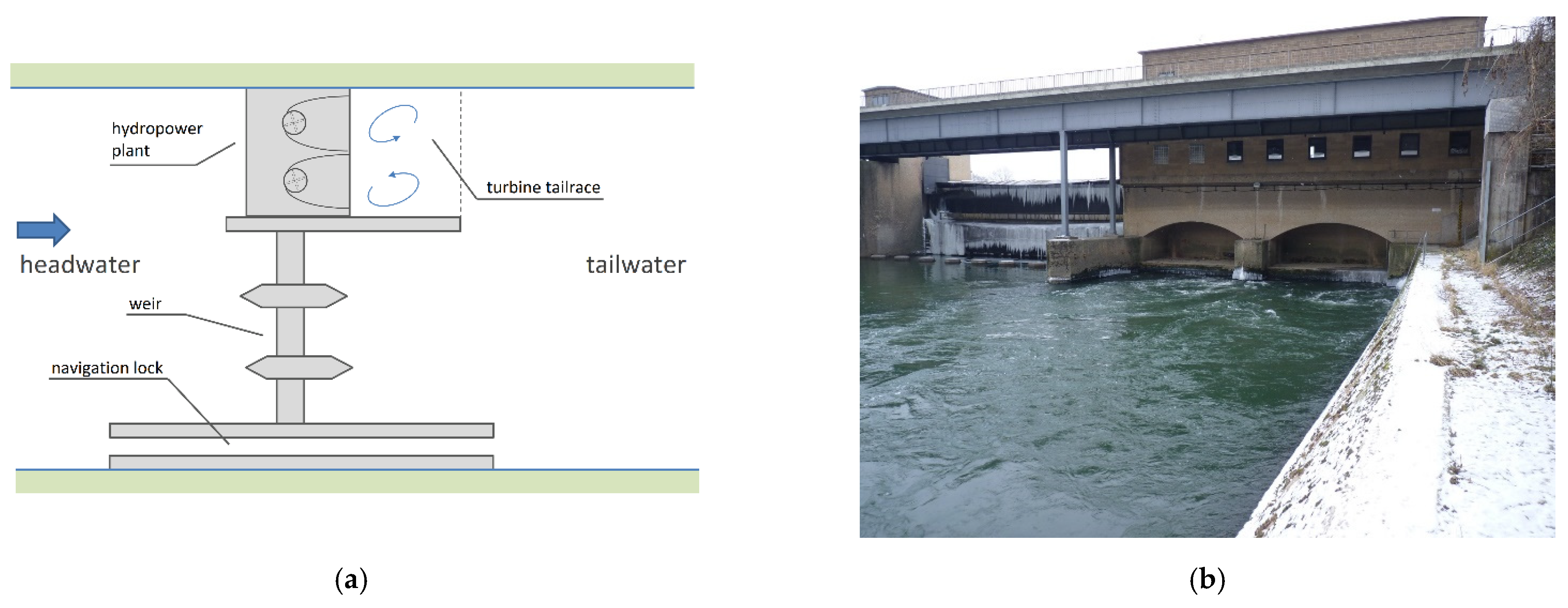
Most of the approximately 100 dams with HPP in the German federal waterways system do not include functional fishways. The average annual flow of these rivers ranges from tens to 400 m3/s which mirrors the approximate design discharges of the respective HPP. A typical design of a dam with navigation lock, weir and HPP and an example of a turbine tailrace are shown in Figure 1.
Highly turbulent flows occur immediately downstream of the draft tubes (turbine tailrace) as turbine releases impact the solid boundary of the channel and energy dissipation structures (if they occur) used to protect the river channel from erosion. Although draft tubes are used to convert kinetic energy into static pressure energy, and consequently to reduce flow speed, mean velocities at the draft tube exit section are still in a typical range from 1 to 2 m/s. Tailrace water velocities are not homogenous, but can vary substantially over time and space as the dynamic, helical discharge from each turbine interacts with discharges from neighboring turbines and with the channel solid boundary forming vortices and turbulent structures of a range of sizes [19,20,21]. Typical surface-observable features of mixing processes in the tailrace are boils, eddies, and reverse flows which vary in size and energy over space and time (Figure 1b). Boiling results from vertical movements of the flow and is observed downstream of the draft tube exit section at discharges higher than 70% of the turbine design discharge [22]. Reverse flows are observed at the water surface near the draft tube exit section [13]. For brevity, we refer to this highly turbulent area as the turbulent zone (TZ). Per definition, the downstream extent of the turbulent zone ends where vortices and turbulent features have largely dissipated and most water velocities are in the direction of the main river flow.
2.2. Design Criteria
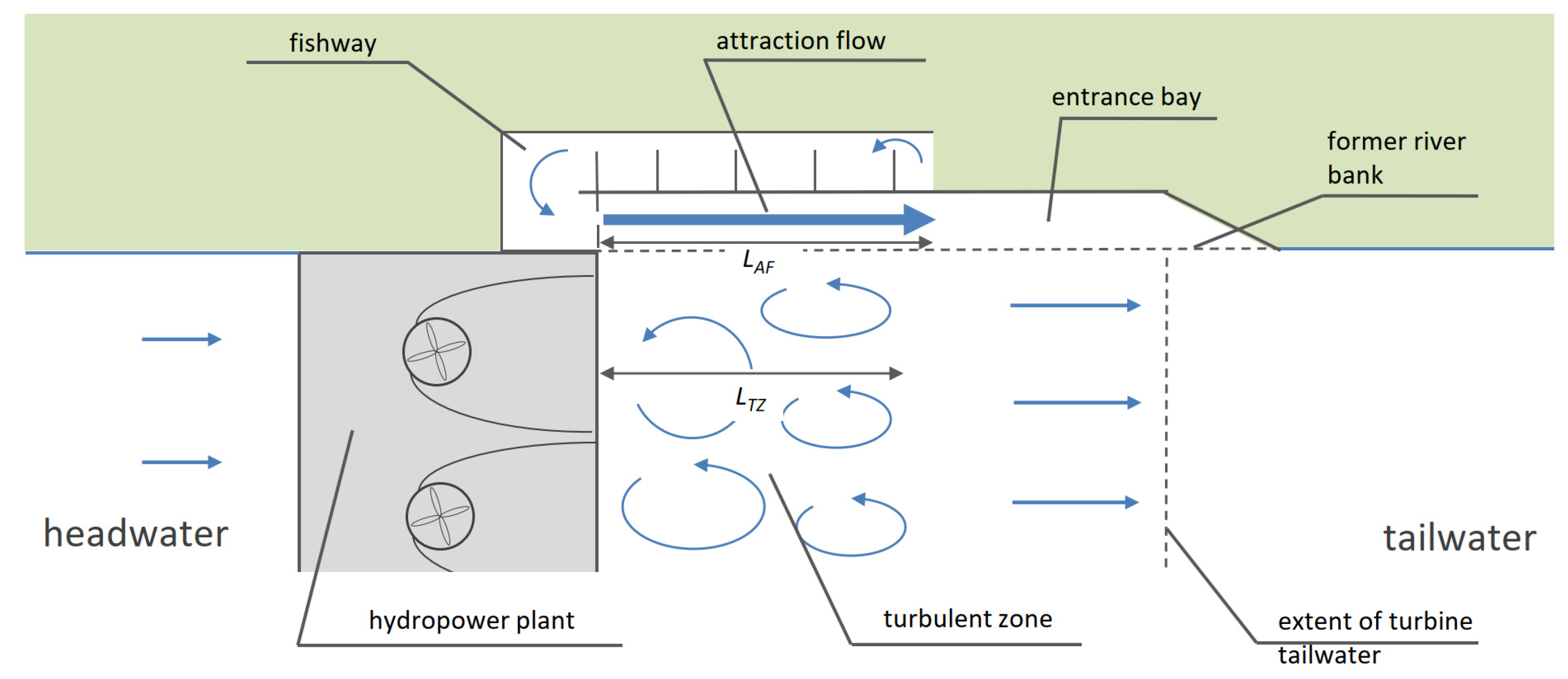
Developing the parametric approach, we start with the current state of the art for the construction of fishways in Germany. The following specifications are particularly important (Figure 2):
- The attraction discharge should be sufficiently large to prevent the intrusion of turbulent structures associated with turbine operation into the fishway entrance bay. A sufficiently large attraction discharge creates an uninterrupted directional signal that guides fishes towards the entrance and reduces the presence of constantly changing flow vectors which may disorient or hinder the movement of fish towards the fishway entrance, particularly at high discharges [10,23,24].
Moreover, the approach requires to establish additional detailed criteria based on fish ecological considerations, literature findings describing fish behavior during migration and aspects of technical feasibility:
- 4.
- A migration corridor for fish approaching the HPP should be located laterally to the turbulent zone (see entrance bay in Figure 2).
- 5.
- Minimum time-averaged water velocities of the attraction flow, , must (a) significantly exceed the rheotaxis threshold to give a clear signal to migratory fish [8,25] and (b) not exceed design water velocities of the fishway. For our approach, we assume to be 0.8 m/s. The attraction velocity considers design recommendations for entrance velocities of fishways [10,16,26] and investigations on flow perception of fish and their swimming behavior and performance [27,28,29].
- 6.
- Water velocities of the attraction flow must be comprised solely of positive flow vectors to not distract fish [7].
- 7.
Since fishways in Germany must be operational at least 300 days during a year [10], we evaluate Equation (1) for hydraulic conditions between and , where is the river discharge and n are the average annual number of days at which the discharge is not exceeded. Generally, HPP design discharges are within this discharge range. We assume that meeting Equation (1) at will also meet the length requirement for all intermediate discharges between and because the most critical turbulent conditions in the tailrace occur at design discharge of HPP.
2.3. Length of Turbulent Zone
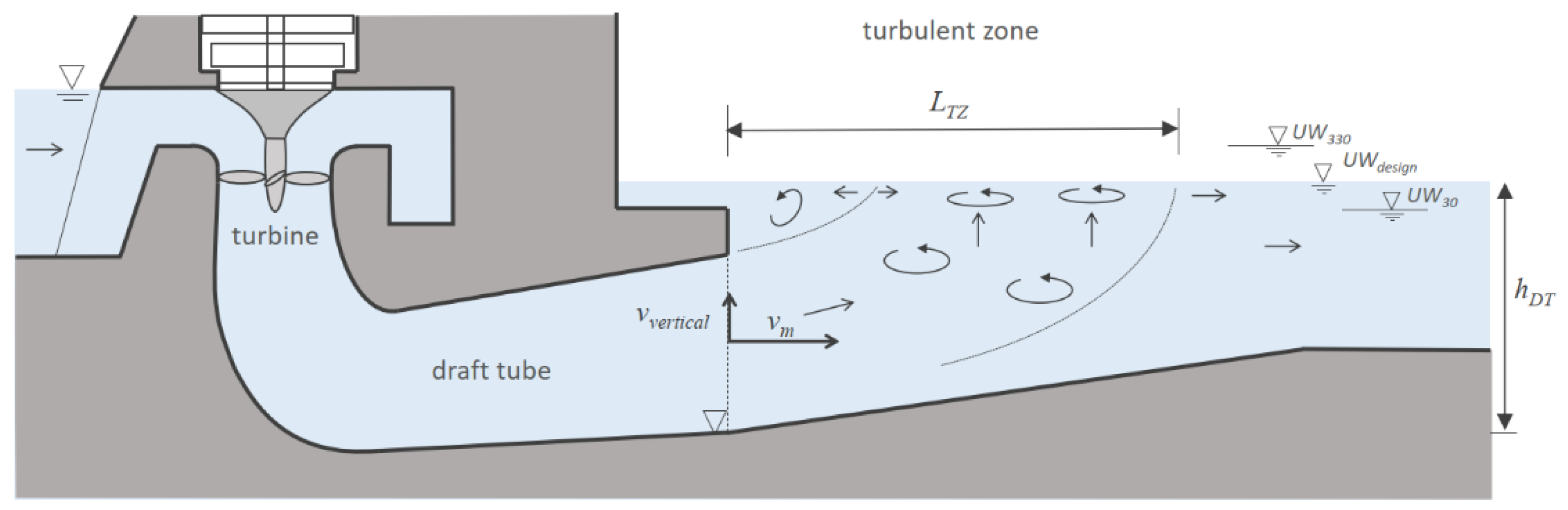
The turbulent zone with observable boiling and vortices in a turbine tailrace depends on the swirl flow emerging from the turbines which is significantly influenced by design features of the draft tube such as elbows and splitter walls as well as channel geometry. It is difficult to accurately simulate the hydraulic effects of all of these features with computational fluid dynamics at the scale at which fish make movement decisions. Even if such studies could be accurately conducted, the interpretation of the results is equally difficult because the biological response of most fish species is largely unknown. We decided to develop an analytical equation to approximately estimate the downstream length of the turbulent tailwater zone in keeping with the principle of parsimony employed in our approach. Vortices generated in turbine and draft tube are transported in vertical and longitudinal direction into the tailrace. Considering the flow propagation, we assume that lengths and velocities in the tailwater near the river bank behave similarly, so that the ratio of and (defined below) is equal to the ratio of bulk exit velocity and vertical velocity caused by the helical nature of the discharges from the draft tube (Figure 3). Above all, we assume that lateral propagation is of minor importance for the bankside turbine as the river bank acts as a geometrical constraint preventing lateral expansion. This allows us to represent the length of the turbulent zone as
and
where, is the water depth at the draft tube exit section when HPP design discharge equals river discharge, is a vertical velocity at the draft tube exit section, is the number of turbines, and is the mean cross-sectional area of the draft tube exit section.
The vertical velocity is unknown and cannot be easily assessed. To obtain we calibrated Equation (2) with direct observation of the length of the turbulent zone. We inferred that the most downstream location in the tailrace, where boils and reverse flows at the water surface are observable, demarcates the downstream extent of the turbulent zone. Four experienced hydraulic engineers assessed the water surface during HPP design discharge and gave an independent estimate. The most downstream estimation was chosen to ensure a conservative estimate. The longitudinal distance to the draft tube exit section () was measured directly at the river bank during the assessment. This procedure was applied at a total of 13 different HPPs at turbine design flow conditions (Table 1). HPP parameters were obtained from the hydropower operators, tailwater levels were retrieved from the hydrologic information system FLYS 3.2.1 (Federal Institute of Hydrology, Koblenz, Germany).
The observed length of the turbulent zone was normalized with the water depth at the draft tube exit section and then plotted against the design bulk velocity of the draft tube exit section (Figure 4). The data were separated by turbine orientation because their flow characteristics differ. The gradient of the least squares linear fit without zero offset represents the reciprocal value of the vertical velocity which we estimate to be 0.56 m/s for VMT with elbow draft tubes and 0.70 m/s for HMT with straight draft tubes. For HMT we use a point estimate because of the limited number and short range of observations. Deviation of the points from linear may be explained by (1) the subjective nature of the observations, (2) missing parameters such as draft tube or channel geometry and other site-specific attributes, and (3) limited number of observations and short range of conditions for HMT.
2.4. Propagation Length of Attraction Flow
2.4.1. Turbulent Rectangular Surface Jet
We simplify the attraction flow as a turbulent, rectangular surface jet corrected for the influence of slot geometry, wall presence and concurrent flows. To calculate the distribution of time-averaged velocities of the attraction flow, we enhanced an existing jet propagation model [32] to meet the boundary conditions present at the entrance of a fishway. Briefly, a three-dimensional jet from a rectangular opening may be classified into three distinct zones when regarding the centerline velocities: a potential core zone, a two-dimensional zone and an asymmetric zone [33,34,35,36]. The transition between the different zones may be calculated as a function of turbulent mixing processes. In [32], the inner diffusion angle is introduced as a measure for the lateral spreading of a jet which is in a range from 4.0° to 5.5° for two-dimensional, axisymmetric jets. For surface jets, the water surface is commonly modelled as symmetry axis neglecting turbulent free-surface currents due to anisotropy of Reynolds normal stresses [37].
Assuming is the centerline axis at the surface, and the initial jet velocity at , the transition coordinate between potential core zone and two-dimensional zone is
with being the width of the rectangular opening, i.e., (with being the height of rectangular opening) and the inner diffusion angle. The transition coordinate between the two-dimensional zone and axisymmetric zone is
The velocity decay for the two-dimensional zone is proportional to and for the axisymmetric zone [32,34]. Consequently, the piecewise function for velocity distribution along the centerline axis may be calculated as
We specified a value for in our test cases using numerical simulation for various aspect ratios [38].
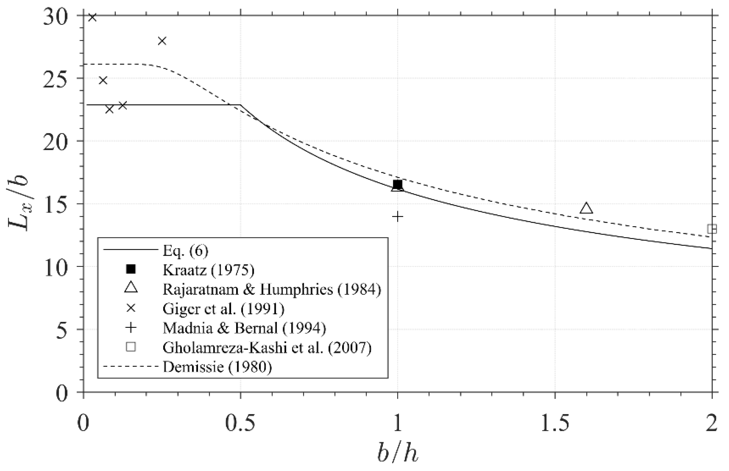
We use Equation (6) to determine the propagation length of a jet emerged from fishway slots with arbitrary aspect ratios . In Figure 5, the half-length of turbulent rectangular surface jets , where velocities on the centerline axis are half the initial velocity, , are calculated for typical aspect ratios of fishway entrances and compared to results from physical or numerical simulations [32,39,40,41,42]. Additionally, a function based on the point-source concept for the half-length is plotted [43]. The comparison yields a good agreement, but with a tendency of underestimation.
2.4.2. Correction for Ambient Flow
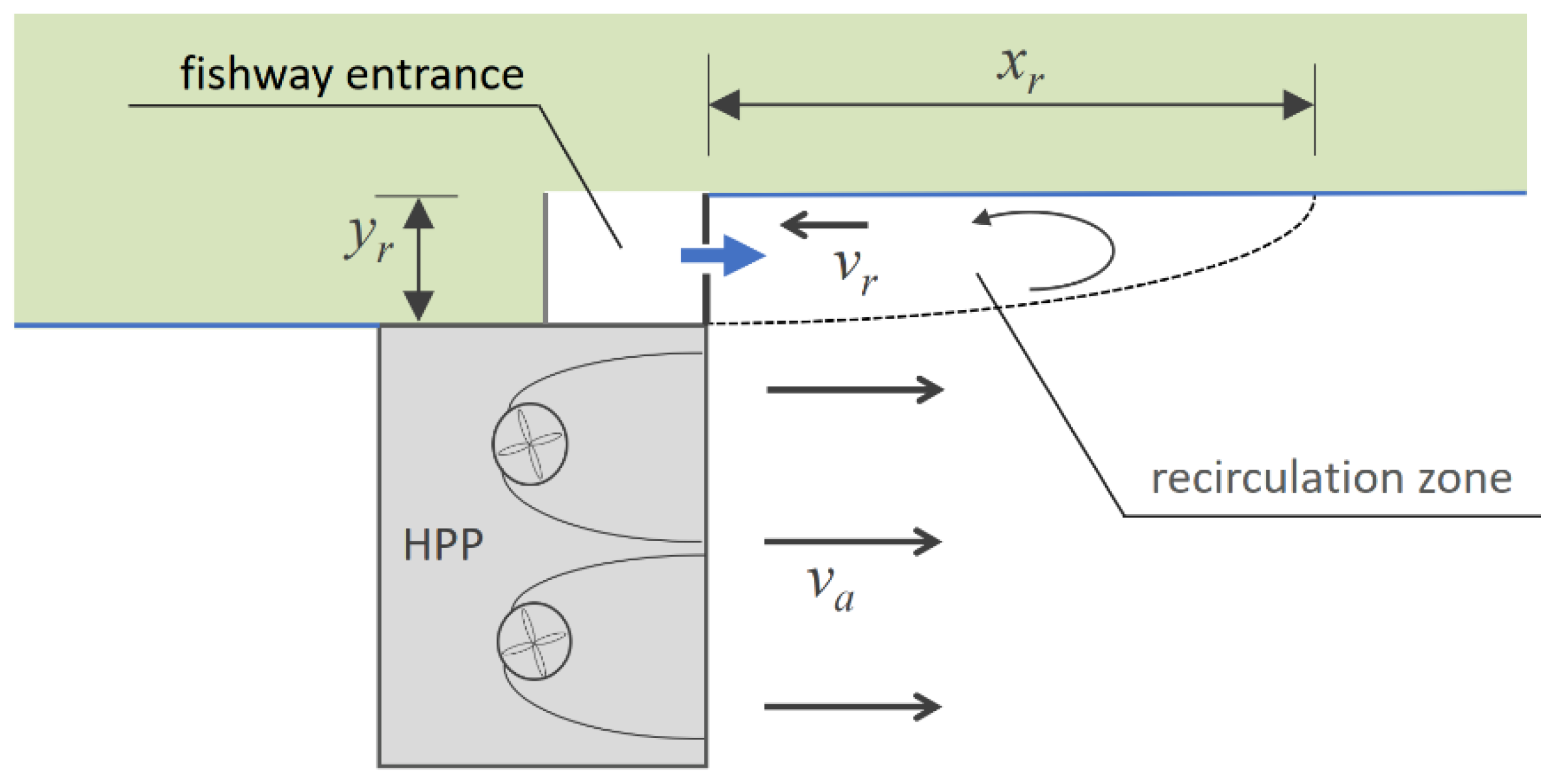
The attraction flow is introduced into an inhomogeneous and highly turbulent tailrace. In the entrance bay stationary eddies result in reverse flows at the river bank. Reverse flows in the entrance bay reduce the average velocity of the fishway attraction jet and consequently result in a shorter propagation length (Figure 6).
We simplified the actual flow field to an ideal two-dimensional case although it is really highly three-dimensional, and validated this approach with detailed 3D numerical simulations of an actual tailrace (see below). In this estimation flow processes in a tailrace are similar to those present in backward-facing steps in a homogeneous flow field. According to [44,45], for a backward-facing step of distance , the length of the recirculation zone at high Reynolds number conditions is
Maximum reverse flow velocities present in a large region of the recirculation zone may be roughly estimated [45,46] as
with being the ambient velocity. Typical values for in tailraces are 2–3 m which results in recirculation lengths of about 10 to 21 m. At turbine design flow, bulk mean velocities at the draft tube exit are in the range of 1–2 m/s, thus reverse velocities may be in a range of 0.2–0.4 m/s assuming this flow is representative of the ambient tailrace velocity .
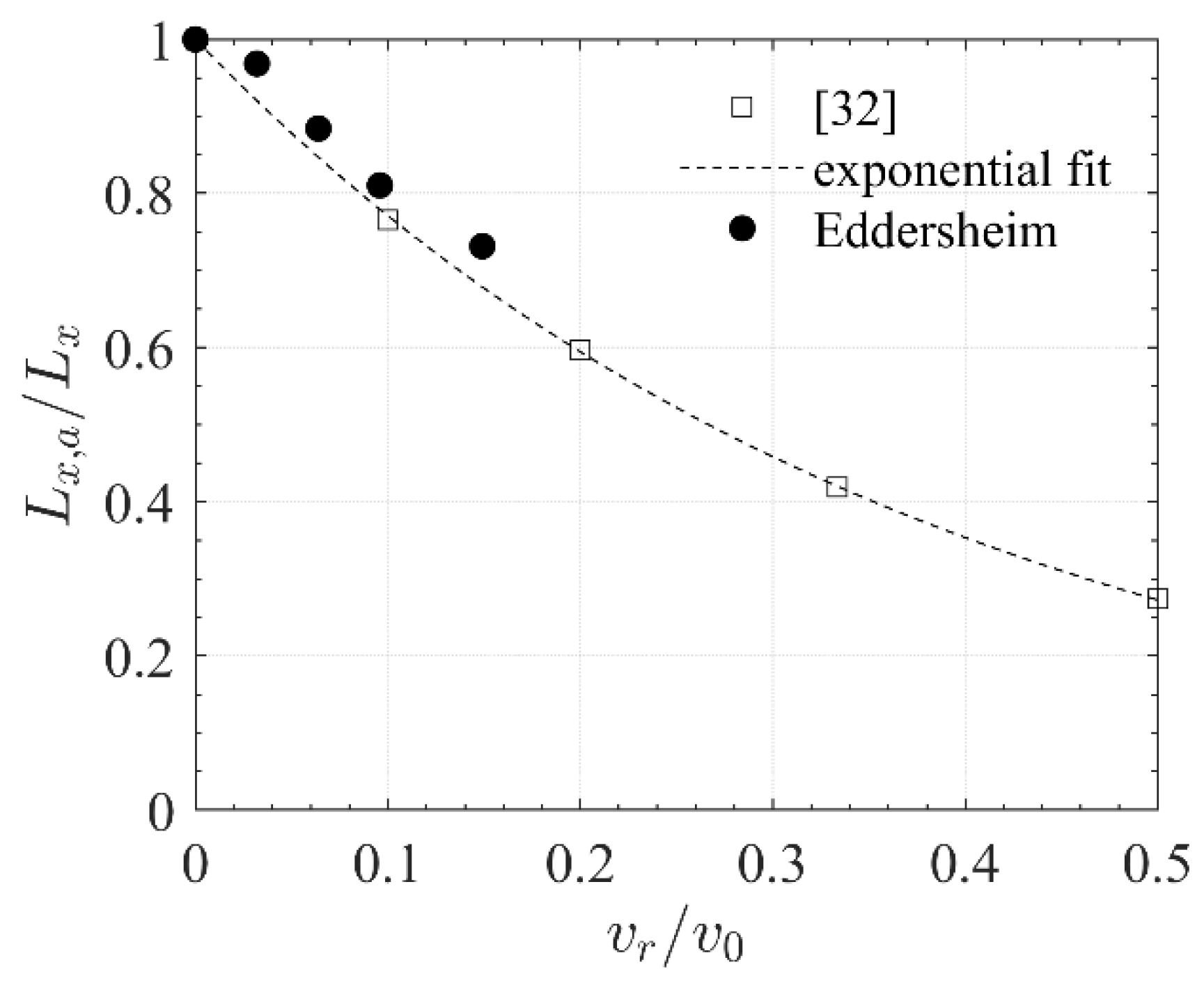
We used investigations reported in [32] to assess the effect of reverse flow on propagation length of the turbulent surface jet. For free symmetric jets with exit velocity in homogeneous reverse flows with velocity , the reduction of the propagation length compared to a free jet in quiescent water can be obtained from nomograms for arbitrary velocity ratios . Approximation of values from the nomogram at gives an exponential relationship
Besides mean reverse flows, large-scale turbulence also shortens propagation length of the fishway discharge plume [47,48,49]. Although turbulent fluid particles typically protrude from the draft tube outflow into the fishway entrance bay, it is not possible to analytically estimate the effect of turbulent processes on propagation length. As a consequence, we used the conservative approach of applying the estimated maximum reverse velocity along the entire length of the attraction flow to account for the effect of turbulence.
We performed 3D-hydrodynamic simulations of the tailrace at Eddersheim Dam located at the Main River in Germany to verify our approach for estimating the propagation length of the fishway discharge flow with concurrent turbine discharge. Details of the numerical methods are given in Appendix A. We varied the turbine discharge so that took values from 0 (no discharge) to 0.15 (design discharge). The outlet velocity of the fishway entrance was held constant at , and was obtained by Equation (8). For each discharge, we measured the length of attraction flow where , and plotted results against the velocity ratio (Figure 7). We obtained good agreement between analytical and numerical estimates of propagation length with a slight tendency to overestimate the reduction with the analytical approach.
2.4.3. Correction for Slot Geometry and Lateral Wall
The investigations on jet propagation described above assume the most upstream velocity profile is homogenous. However, hydraulic conditions at fishway entrances differ because (1) flow in entrance pools is highly turbulent and inhomogeneous, (2) the entrance consists of a vertical slot instead of nozzles (which have been comprehensively investigated [32,36]) and (3) typical entrances are located near solid boundaries (e.g., river banks or concrete walls) that may influence jet propagation. To quantify the impact of these boundary conditions on the attraction flow, numerical simulations of differing slot geometries and lateral wall presence were performed [50]. It was found that the propagation length of jets emerging from vertical slots with inhomogeneous and turbulent upstream conditions show reduced propagation. In contrast, presence of lateral walls located at a distance from the slot extends the length of the attraction discharge jet.
The complexity of flow through a fishway entrance slot and the number of parameters that influence the propagation length of a turbulent jet prevents the formulation of a one- or two-term analytical solution. Therefore, the effects of these parameters on propagation length are represented by a conservative, constant correction factor of 1.2 (in accordance with [50]). In order to use a constant factor, it is necessary to define that the entrance slot must be located at a lateral distance of one slot width from the river bank or a lateral wall.
2.5. Determination of Width of Entrance Slot and Attraction Discharge
Using Equations (1) and (6), the width of an entrance slot to provide the required attraction flow is calculated as
where is a form factor of the jet propagation; and are correction factors for the fishway entrance configuration; is the inner diffusion angle of the rectangular surface jet; m/s is the minimum attraction velocity; and is the design velocity of the entrance slot. The form factor is calculated as
where is the downstream water depth at the entrance slot during an HPP discharge of . The correction factor adjusts for the effect of reverse flows as
We consider the effect of entrance geometry on the propagation of the attraction flow to be represented as a constant factor of . For a given slot width , attraction discharge may be roughly calculated to
where denotes the water depth downstream of the slot, and is the discharge coefficient of the slot. To be consistent with slot hydraulics in the fishway (e.g., meet the velocity thresholds) we assume that the coefficient for the entrance slot is equal to those of the fishway slots. We chose according to the established coefficients of vertical slot fishways [10]. The design velocity of the entrance slot is calculated with the design head loss as
This velocity should be kept constant for varying tailwater levels in order to maintain a well-defined attraction flow e.g., by adding auxiliary discharge into the entrance pool.
3. Results
3.1. Attraction Discharge
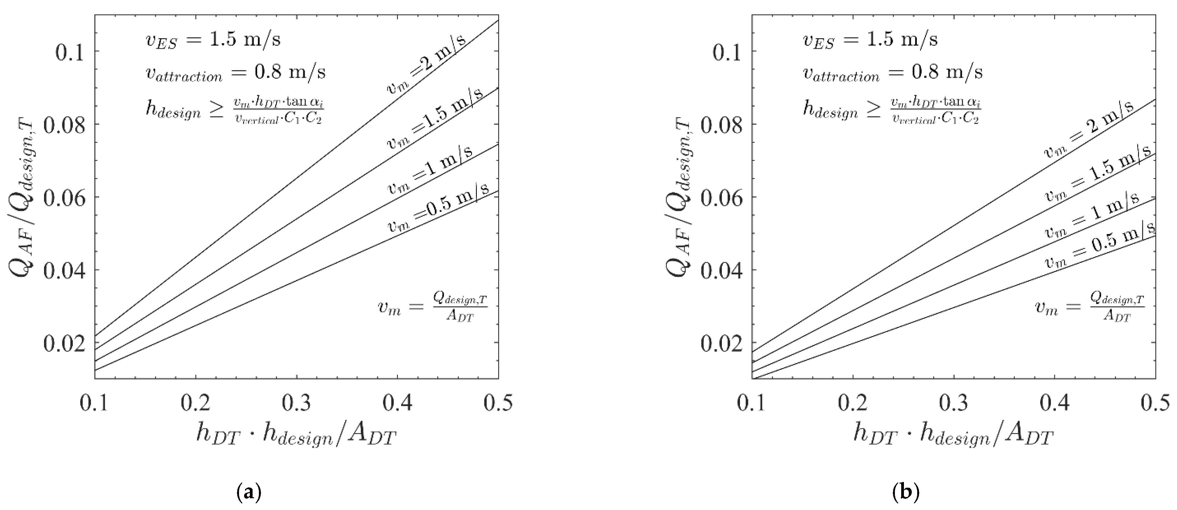
Our approach is depicted in Figure 8 as a nomograph for when water depths in the entrance are sufficiently large compared to the length of the turbulent zone (see Equation (11)), and the attraction flow from the HPP propagates primarily as a two-dimensional surface jet. We assume an entrance velocity which is typical for German federal waterways. The resulting attraction discharge is normalized by the design discharge of a single turbine and the bulk velocity at the draft tube exit can be represented by an array of curves.
The required attraction discharge can be calculated within a range of 1 to 10 percent of the discharge of a single turbine depending on the geometric and hydraulic conditions at the site. For example, fishway attraction discharge increases linearly with entrance flow depth (or water depth) and with higher bulk velocities at the draft tube outflow. In contrast, effective attraction discharge decreases if mean outflow velocities are reduced or if the cross-sectional area of the draft tube exit increases.
3.2. Case Study
We apply our methodology to four dams of the German federal waterways system, where fishways are currently being planned (Table 2). These dams have been the target of detailed physical and numerical hydraulic models to determine slot geometries and fishway attraction discharges [9,51,52,53] against which we can compare our parametric approach. A summary of the respective investigations for all study sites is given in Appendix B. Boundary conditions at Lauffen, Kochendorf and Wallstadt Dams agree with those given in Section 2.2, notably the entrances into the fishways are located directly lateral to the draft tube exit sections, an entrance bay is located laterally to the tailrace, and attraction flows are released in the turbine tailrace. Attraction discharge is regulated depending on the tailwater level in order to provide constant water velocities at the entrance with the exception of Lehmen. There, the attraction discharge is kept constant and the water velocities in the fishway entrance are regulated by a sluice gate controlling the flow height.
Using our methods and the input data of Table 2, we calculate the lengths of the turbulent tailwater zone, widths of the entrance slots, and fishway attraction discharges for each location and for tailwater levels , and (Table 3). For the Lehmen Dam it is necessary to estimate some of the values (e.g. bottom of entrance slot) because these values are not available. The results are compared with those derived from detailed numerical or physical investigations for the case study locations and also with values calculated by the conventional simple methods described in the Introduction. For this purpose, we use standard values to parameterize the simple methods as follows:
- One percent and 1.5% as lower and upper estimates, respectively, of the design discharge of the entire HPP as proposed for French rivers [14].
- Five percent of the design discharge of the turbine adjacent to the fishway as proposed for German Waterways [17].
- Five percent of the maximum HPP discharge proposed for rivers in the UK [16].
These results should be understood as maximum discharges which are usually needed at high tailwater levels during .
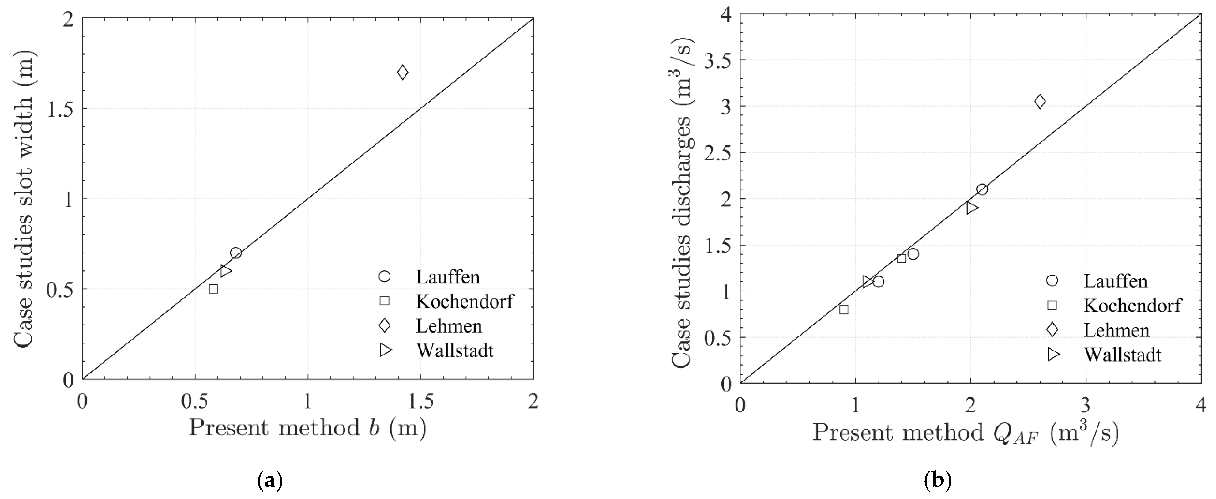
Our calculated slot widths and attraction discharge agree well with the values derived from numerical and experimental simulations for Lauffen, Kochendorf and Wallstadt (Figure 9). Our maximum slot width deviation is 0.08 m or 15%. Our maximum deviation for attraction discharges is less than 0.2 m3/s or approximately 12%.
At Lehmen Dam, we can only compare our results to detailed studies at when the flow heights in the fishway entrances are comparable to our case and with constraints imposed by our approach. We underestimate slot width by 0.28 m or 17% and corresponding attraction discharge by approximately 22%. Given the complexity and the overall uncertainty we consider our approach to be robust and conclude that our method leads to plausible fishway design parameters.
The discharge recommendations from the selected simple approaches differ substantially among each other. Discharges recommended for our case sites using the UK method [16] are about 3 to 5 times higher than recommendations using the French method [14] while values from the method for German Federal waterways [17] are in between. Consequently, our estimates of fishway attraction discharge in some cases match the results from the simple methods (using the approach for German Federal Waterways at Lauffen [17] or the estimate for French rives in Wallstadt [14]) and in some cases deviate strongly (using the UK approach at all sites [16], the French approach at Lauffen and Lehmen [14], and the German Federal Waterway estimates [17] at Wallstadt and Lehmen).
4. Discussion
4.1. Design Approach
At several stages during the development of the parametric approach we had to decide whether to move ahead with a simplified estimation or to further deepen the understanding of physics behind the processes. However, in order to reach the goal of a transparent and reliable method which can easily be applied to a large number of different dams and rivers it was necessary to reduce the complexity of the methods applied. The proposed approach may therefore be considered as a first step towards this goal. The overall framework of the approach provides the possibility to further enhance the underlying methods, to introduce further metrics or to decide for deviating coefficient values. This applies in particular to the quantification of the turbulent zone and the jet propagation.
The outcome of the visual measure used to calibrate Equation (2) can be influenced by the actual hydraulic conditions, observation angles and individual perception. It is advisable to report the process and the site-specific conditions in a detailed protocol to enable the replicability of the results. The standard deviation of the individual length estimates given by the four experts involved was less than 5% of the estimated value for most of the dams and maximum 15% at two dams with ambiguous tailrace characteristics. No other easily applicable methods are yet available to measure the length of the turbulent zone. More sophisticated velocity measuring techniques capable to quantify turbulent fluctuations in a tailrace often fail for practical reasons e.g. availability of steady flow conditions, accessibility of the tailrace, or for operational safety aspects in the vicinity of the turbines. Furthermore, despite the availability of several frameworks that combine fish movement and turbulence [54,55], there is no translation of the measured hydraulic values that correspond to fish perception. Thus, we are still not able to exactly define turbulence limits for fish in realistic tailraces and consequently to determine the length of the turbulent zone. Ultimately, the formulation of a universal relation fails because of differences in individual fish performance. Therefore, the proposed Equation (2) in combination with calibration at a number of different dams seems appropriate as basis for our approach, especially when it is necessary to estimate attraction flow for a great number of sites and thus support program scale decisions. It is acknowledged that further observations at other dam locations may increase the reliability of the assessment, especially for horizontally mounted turbines where only few observations have been possible.
The modelling of jet propagation required additional investigations and definitions to account for the relevant influences. While some of the processes are widely investigated (jet propagation) factors like reverse flow and slot wall correction needed to be customized for the specific boundary conditions at fishway entrances. Here, simplification was also indispensable. Regarding the manifold dam locations at German federal waterways we concluded that exact and detailed representation of entrance and tailrace geometries would not facilitate a practical approach. For example, the effect of reverse flows in the tailrace on the attraction jet was considered by a simple two-dimensional analytical approach. Parameters that were not considered in detail are: vertical and lateral offset of the attraction jet, inclined ramps downstream of the entrance slot, velocity distribution and turbulence characteristics of the turbine outflow, among others. However, including conservative assumptions in our approach we could establish a consistent formulation that shows good agreement to detailed numerical simulation that was used for validation.
The effect of slot geometry and its lateral distance to an adjacent wall also was found to have an important impact on jet propagation [50]. Most efficient in terms of propagation are slots close to a lateral wall because the jet attaches quickly to the wall and propagates further downstream. For our approach we decided to use a typical distance of one slot width as maximum permissible distance to the wall and established a correction factor accordingly. For smaller distances the approach is conservative since a faster wall attachment results in increased propagation. However, a minimum distance between jet and wall will allow fish to approach the slot from either side without having to navigate the jet directly, which will save energy during the ascent [56]. Larger distances between slot and wall are not covered by the present approach. They would require a smaller correction factor resulting in an increase of attraction discharge to propagate as required.
4.2. Validation
Despite the above discussed necessary simplifications resulting attraction flows for the four dams of the case study were found to be in good agreement with the discharge recommendations from the detailed models, especially if the construction and arrangement of the fishway entrance meet our requirements given in Section 2.2. In this case, maximum deviations for slot width and attraction discharge were less than 15%.
In contrast, our results show that attraction discharges obtained from simple methods (calculated by percentages of competing discharge only) sometimes match the results from detailed models but more often deviate as far as ±40 to 50% (see Table 3). The definition of competing discharge is considered as the main reason for the variability regarding the attraction flow obtained from simple methods. Using a proportion of average annual daily flow for attraction discharge, [16] follows the idea that at larger rivers more discharge from the fishway is needed to attract fish. However, as shown by [9] even a large attraction discharge can only affect the tailwater section close to the bank. The geometrical shape of the river bank can be very similar at rivers of very different sizes, so that an attraction flow solely based on the total river runoff may have very different effects. Using a proportion of the maximum design flow of the HPP for attraction discharge follows the idea that the fishway needs to compete with the total HPP outflow since it is the most attractive part of the river for upstream navigating fish [14]. For propagation of the attraction flow, the maximum design flow of the total HPP is less important than the flow through the turbine close to the bank, though. Thus, an attraction discharge calculated as a proportion of total HPP outflow will work out very differently depending on the total number of turbines. Using a proportion of the maximum flow of the turbine next to the fishway takes up the idea that attraction flow mainly affects the area close to the bank and additional turbines do not increase the required attraction discharge [9,17]. Although this approach is closer to our method it does not take turbine characteristics into account that may influence flow velocities in the tailrace and act differently on the attraction flow. A draft tube regains potential energy by reducing kinetic energy of the flow [22], so that less attraction flow is required at locations with more efficient draft tubes having lower mean flow velocities and a shorter turbulent zone.
Besides competing discharge, other important factors influence shape and length of the attraction flow, mainly slot geometry, and velocity at the fishway entrance slot. The simple approaches neither explicitly consider these factors nor do they limit the application to specific geometric and hydraulic conditions of the entrance and tailrace (comparable to design criteria given in Section 2.2). In summary, we find that the resulting attraction flow of the simple approaches only agree with those of complex models if the essential geometric and hydraulic conditions coincide by chance, which is the case at the Lauffen Dam when compared to [17] (Table 3).
Based on these considerations and given the assumption that from the methods compared the detailed approaches provide the best representation of reality, we can attest our parametric approach an approximation that is closer and significantly more consistent than the results of the simple approaches and easier applicable than sophisticated modelling.
4.3. Significance in the Context of Planning
Our approach, because of its simplicity, allows planners to determine the necessary fishway attraction discharge early in the planning process and, thereby, prevent major revisions to dam design later in the planning process when many features of the dam have already been established. This is particularly important when operating discharge of the fishway is insufficient to provide effective attraction flow and must be supplemented by auxiliary water. Auxiliary water for attraction, which may be substantial, is usually introduced into the pool immediately upstream of the entrance slot [10]. The extensive structures associated with the auxiliary water supply (upstream intake, piping, screens to prevent fish entry into the water supply pipe, energy dissipation structures, maintenance access, and valves to regulate the quantity of auxiliary flow) also have to be considered [57]. Identifying the need for auxiliary water early in the planning process reduces cost and increases planning efficiency.
However, further work is needed to evaluate our approach for HPPs that are larger than the mid-sized dams that are the focus of our studies. Our approach may not apply for large dams with extended turbulent zones (>20 m) because more than a single fishway entrance located near the draft tube outflows may be needed to meet fish passage goals. The required attraction discharge increases substantially in such cases and slot widths of 1.6 m or larger may be needed. An increased requirement for auxiliary water supply could raise problems concerning the availability of water, the integration of the auxiliary water system with other project infrastructure, and other site-specific issues such as provision for maintenance and repair of the fishway. Consequently, for large rivers outside the range of our case-histories it may be better to provide a second fishway entrance either downstream of the main entrance or on the other side of the HPP [26].
At small HPPs with a shortened turbulent zone, low discharges, and small tailrace dimensions, our approach may determine slot widths that would be smaller compared to ecological requirements necessary to meet fish passage goals (e.g., minimum slot width according to target species). In these cases, our parametric approach shows that operational discharge of the fishways already provides a sufficient attraction flow and that an auxiliary water supply is not needed.
5. Conclusions
The German Federal Waterway and Shipping Administration (WSV) is faced with the major challenge of restoring river continuity at a large number of dams without fishways in German waterways. Our approach is a step towards development of an objective and reliable method to determine attraction flow for fishways that can be applied to many dams at a program scale to meet the requirements of the water frameworks directive. The approach enables recommendations for fishway attraction flows for dams of different locations and sizes using easily obtained site specific information. By incorporating tailrace flow patterns more accurate discharge estimates are possible than methods using solely HPP or dam flow summaries as are presently used. Comparison of our results to four different dams where attraction discharge was determined using detailed hydraulic studies show good agreement for width of the entrance slot and the attraction discharge. We acknowledge our approach still leaves uncertainties that are not completely addressed including the length of the turbulent zone in a turbine tailrace and the effect of turbine discharge on the propagation of the attraction flow, among others. We anticipate that further investigations at three pilot locations currently in planning at German waterways [58] will identify additional parameters whose use may possibly increase the accuracy of attraction flow and slot width determinations. However, the overall results of our approach are consistent with detailed studies so that we recommend our approach for implementation.
Author Contributions
Conceptualization, P.H., M.Z., C.S., R.B.W.; methodology, P.H.; validation, M.Z.; writing—original draft preparation, P.H.; writing—review and editing, P.H., M.Z., C.S., R.B.W.; visualization, P.H.; supervision, P.H., R.B.W. All authors have read and agreed to the published version of the manuscript.
Funding
This article results from the joint research project “Ecological Continuity of Waterways” of the German Federal Institute of Hydrology (BfG) and the Federal Waterways Engineering and Research Institute (BAW) on behalf of the Federal Ministry of Transport and Digital Infrastructure (BMVI).
Institutional Review Board Statement
Not applicable.
Informed Consent Statement
Not applicable.
Data Availability Statement
Not applicable.
Acknowledgments
The authors wish to thank their colleagues at the Federal Waterways Engineering and Research Institute (BAW) and Federal Institute of Hydrology (BfG): Lena Mahl for performing numerous numerical simulations during this project; Florian Lindenberger and Frederik Prinz for organizing the on-site inspections of the HPP tailwater; Veronica Wiering and Wilko Heimann for supporting the on-site inspections; Martin Henning, David Gisen and Wilko Heimann for discussing the design criteria. John Nestler of the Fisheries and Environmental Partnership made helpful comments on an early draft of this paper.
Conflicts of Interest
The authors declare no conflict of interest.
Appendix A
To validate the influence of the concurrent turbine flow on the propagation of the fishway attraction flow, computational fluid dynamics simulations were performed at Eddersheim Dam, Main River, using the open source toolbox OpenFOAM 4.1 from OpenFOAM Foundation Ltd, London, UK [59]. The transient multiphase solver interFoam [60] was used to model the flow fields employing a volume-of-fluid approach to track the free surface. A Reynolds-averaged Navier–Stokes (RANS) k-ω shear stress transport (SST) model was employed as turbulence model. It combines the advantages of the k-ω and k-ε model by using k-ω near the wall and k-ε in the free flow region [61].
The model domain included the fishway entrance and the tailrace of the three turbines up to 100 m distance as presented in Figure 6. The bathymetry was modeled after data from multibeam echosounder of the river bed. The fishway entrance was located close to the hydraulic power plant, 3 m downstream of the draft tube exit section. The slot width was 0.9 m. The meshing process was similar to that described in [9]. The basic grid resolution was 0.8 m, with refinements in the water zone up to 0.2 m. The water surface, fishway entrance pool and the tailrace of the turbine closest to the river bank were further refined to 0.1 m. The slot walls were refined to 0.05 m. The total grid size was about 6.2 million cells.
The velocity distribution at the vertical draft tube exit plane was calibrated by means of velocity measurements performed with a moving-vessel acoustic Doppler current profiler (ADCP) in the turbine tailrace. A Rio Grande ADCP (Type WHRZ1200-I-UG4 1200 kHz) from RD Instruments was used to record two transects in 10 m and 20 m distance to the draft tube exit plane at a discharge of 70 m3/s of the bankside turbine. Each transect was navigated 120 times and results were averaged to reduce uncertainty due to turbulent fluctuations. During calibration, the draft tube exit plane velocity distribution was adjusted to minimize the root mean square error (RSME) between simulated velocities and measurements in both transects (RSME = 0.13 m/s).
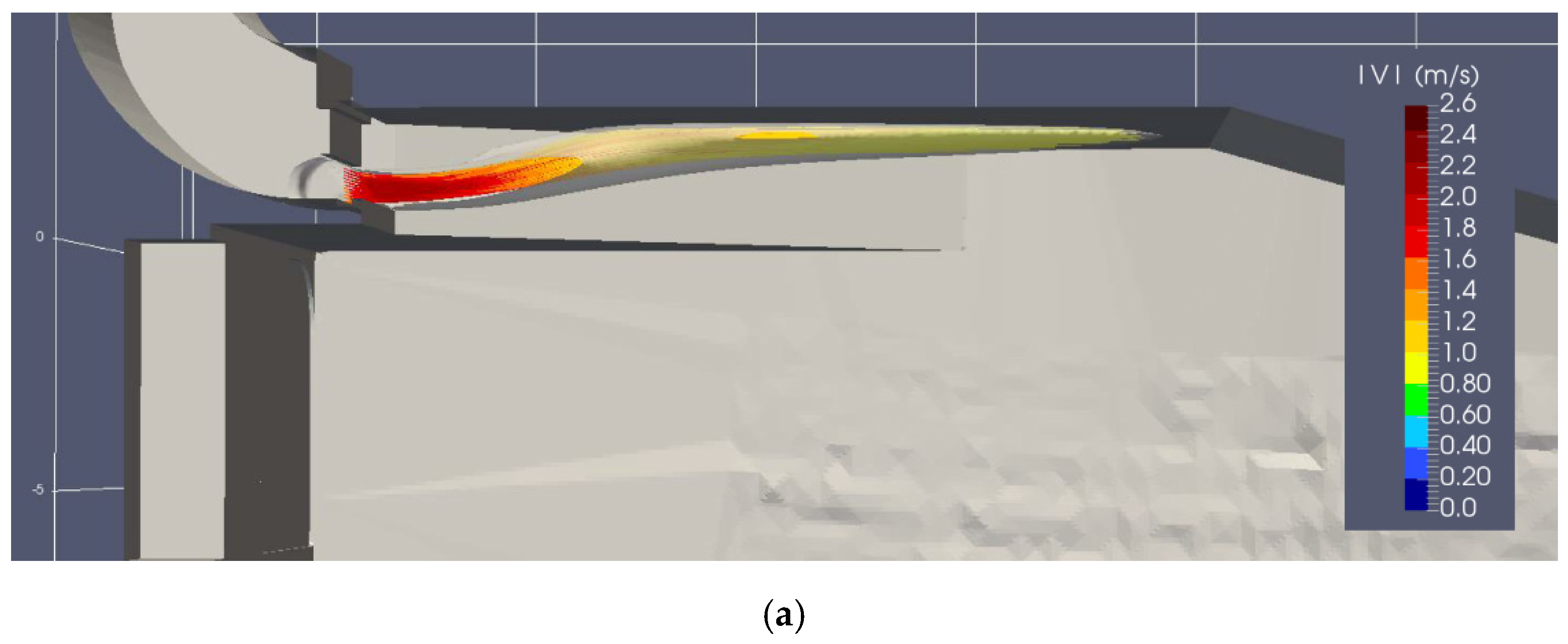
Five different discharge scenarios for the turbine adjacent to the river bank were simulated with the calibrated model: Q = 0, 15, 30, 45 and 70 m3/s. The principal velocity distribution at the draft tube exit section was kept for all scenarios, but the discharge was scaled linearly. Tailrace water levels were constant in all scenarios and attraction flow of the fishway was 1.73 m3/s. Examples of the resulting mean flow field for 0 and 70 m3/s turbine discharge are given in Figure A1.
Figure A1.
Top view of tailrace and entrance bay of the hydrodynamic-numerical model of the dam in Eddersheim (Main River); streamlines of the attraction flow () and the mean flow field of the turbine are plotted for (a) turbine discharge = 0 m3/s, (b) turbine discharge = 70 m3/s.
Figure A1.
Top view of tailrace and entrance bay of the hydrodynamic-numerical model of the dam in Eddersheim (Main River); streamlines of the attraction flow () and the mean flow field of the turbine are plotted for (a) turbine discharge = 0 m3/s, (b) turbine discharge = 70 m3/s.


Appendix B
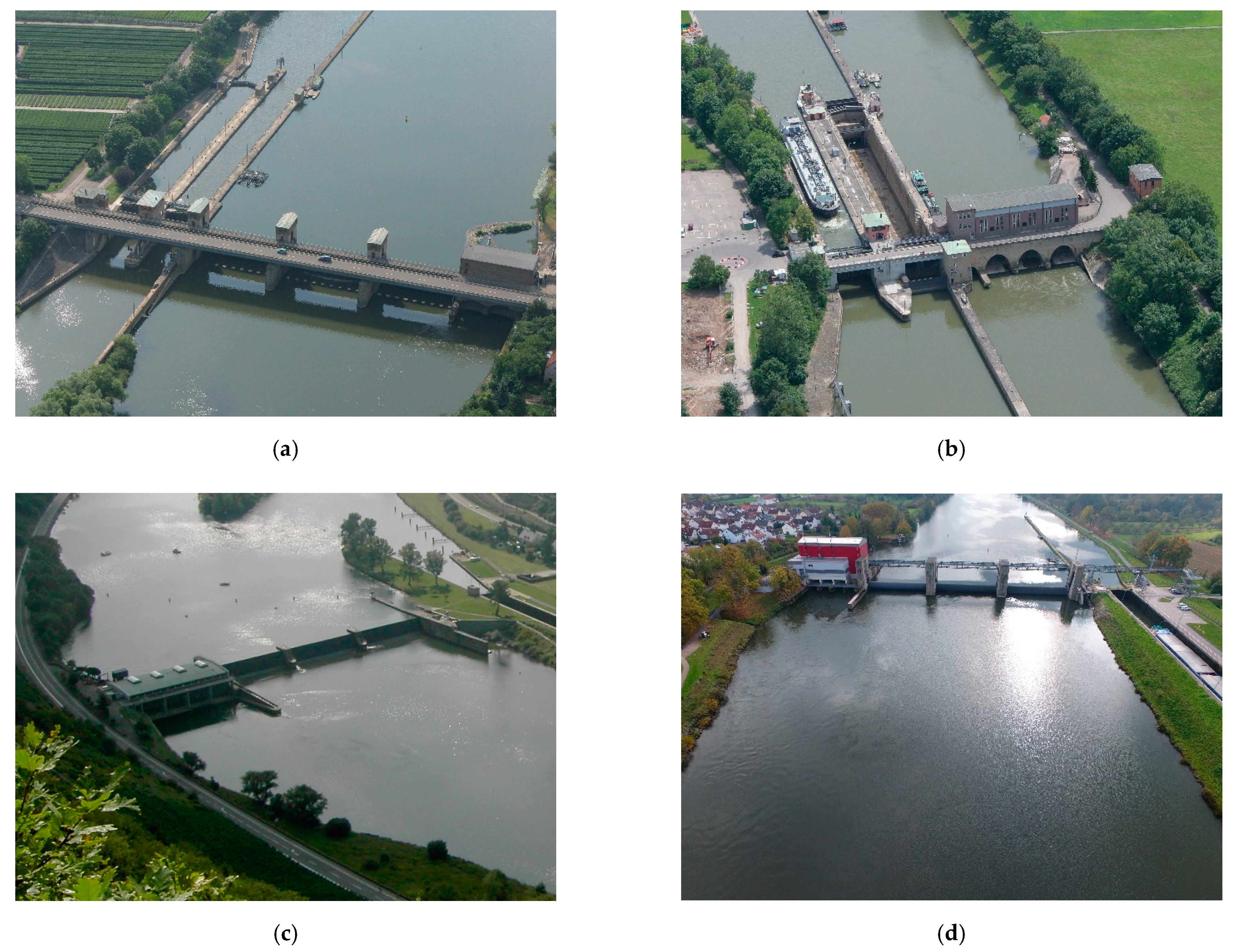
The dams used for the case study are typical dams at German federal waterways (Figure A2). Information about the dams and the investigations to determine attraction flow are described below.
Figure A2.
Aerial photos of dams on the Neckar River at (a) Lauffen and (b) Kochendorf, the Moselle River at (c) Lehmen, and the Main River at (d) Wallstadt.
Figure A2.
Aerial photos of dams on the Neckar River at (a) Lauffen and (b) Kochendorf, the Moselle River at (c) Lehmen, and the Main River at (d) Wallstadt.

Lauffen
Optimum attraction flow for the fishway main entrance at the Lauffen Dam was investigated with a laboratory scale (1:10) model that includes both turbines, their respective draft tubes, tailrace geometry, and the fishway entrance and entrance bay [51]. The entrance is connected to the tailwater bottom by an inclined ramp. Velocity profiles were collected in the tailrace using an acoustic Doppler velocity profiler (ADCP) to calibrate numerical and physical models of the flow characteristics in the near field of the fishway [62]. The flow fields of multiple different entrance configurations and flow rates were measured in the scale model with acoustic Doppler velocimeters (ADV) and evaluated for their ability to provide a suitable migration corridor for migrating fishes. An optimal entrance slot width of 0.7 m, and attraction discharges of 1.1 m3/s for low water levels (), 1.4 m3/s for design conditions of the HPP, and for 2.1 m3/s for high water levels () were determined.
Kochendorf
Effective attraction discharges for a fishway entrance at the Kochendorf Dam on the Neckar River were determined with a computational fluid dynamics model to simulate hydraulic conditions in a tailrace [9,63]. The numerical model domain includes three turbines with draft tubes and the fishway entrance at the bankside draft tube exit section. In contrast to the fishway design at Lauffen, the Kochendorf entrance configuration includes an additional bottom entrance instead of an inclined ramp. Both the near surface and bottom slot are 0.5 m wide. For the simulations, the transient 3D solver interFoam is used where the free water surface is modelled with the volume of fluid (VoF) method and turbulence is modelled with the delayed detached-eddy simulation technique [9]. We conclude an optimized attraction discharge of 1.7 m3/s for high tailwater levels corresponding to is sufficient to ensure a contiguous migration corridor. This discharge is split into a discharge of 1.35 m3/s for the near-surface entrance and to 0.35 m3/s for the bottom entrance. At low tailwater levels, the discharge for the upper entrance opening reduces to 0.8 m3/s.
Lehmen
Computational fluid dynamics simulations were performed to design entrance pools and slots at Lehmen Dam on the Moselle River, a French–German River with annual daily average discharge of approximately 350 m3/s [53]. In contrast to the other case study locations, three fishway entrances are currently planned for this dam, including two near the draft tube and one farther downstream of the turbines. A constant discharge of about 5 m3/s is provided for all three entrances and hydraulic conditions. A sluice gate at each entrance regulates the flow height to ensure a constant velocity for all tailrace water levels. The maximum slot width of the main entrance located near the draft tube is 1.7 m and releases an attraction discharge ranging from 2.5–3.1 m3/s.
Wallstadt
Attraction flow for the fishway at Wallstadt Dam on the Main River was investigated using 3D computational fluid dynamics simulations [52]. The numerical model domain includes two turbines with draft tubes and a fishway entrance adjacent to the draft tubes near the left bank. We use the transient 3D solver interFoam where the free water surface is modelled with the volume of fluid (VoF) method and turbulence is modelled with a statistical k-ω STT model. Turbine and attraction tailwater velocity profiles for model calibration were measured on-site using ADCP. Simulations were performed to evaluate alternative widths of the entrance slot and attraction discharges. Model results indicate an optimized attraction discharge of 1.9 m3/s for high tailwater levels (corresponding to ) with an entrance slot width of 0.6 m produces an acceptable migration corridor. An attraction discharge of 1.1 m3/s produced an acceptable migration corridor for low water levels (corresponding to ).
References
- European Union. Directive 2000/60/EG of the European Parliament and of the Council-Framework for Community Action in the Field of Water Policy: Directive 2000/60/EG-Water Framework Directive; European Union: Brussels, Belgium, 2000. [Google Scholar]
- Larinier, M. Fishways-General considerations. Bull. Fr. Pêche Piscic. 2002, 364, 21–27. [Google Scholar] [CrossRef] [Green Version]
- Venus, T.E.; Smialek, N.; Pander, J.; Harby, A.; Geist, J. Evaluating Cost Trade-Offs between Hydropower and Fish Passage Mitigation. Sustainability 2020, 12, 8520. [Google Scholar] [CrossRef]
- Williams, J.G.; Armstrong, G.S.; Katopodis, C.; Larinier, M.; Travade, F. Thinking like a fish: A key ingredient for development of effective fish passage facilities at river obstructions. River Res. Appl. 2012, 28, 407–417. [Google Scholar] [CrossRef] [Green Version]
- Enders, E.C.; Boisclair, D.; Roy, A.G. The effect of turbulence on the cost of swimming for juvenile Atlantic salmon (Salmo salar). Can. J. Fish. Aquat. Sci. 2003, 60, 1149–1160. [Google Scholar] [CrossRef]
- Čada, G.; Carlson, T.; Ferguson, J.; Richmond, M.; Sale, M. Exploring the Role of Shear Stress and Severe Turbulence in Downstream Fish Passage. In Hydro’s Future: Technology Markets and Policy, Proceedings of the Waterpower Conference 1999, Las Vegas, NV, USA, 6–9 July 1999; Brookshier, P.A., Ed.; American Society of Civil Engineers: Reston, VA, USA, 1999; pp. 1–9. ISBN 978-0-7844-0440-9. [Google Scholar]
- Liao, J.C. A review of fish swimming mechanics and behaviour in altered flows. Philos. Trans. R. Soc. B Biol. Sci. 2007, 362, 1973–1993. [Google Scholar] [CrossRef] [PubMed] [Green Version]
- Pavlov, D.; Lupandin, A.; Skorobogatov, M. The Effects of Flow Turbulence on the Behavior and Distribution of Fish. J. Ichthyol. 2000, 40, 232–261. [Google Scholar]
- Gisen, D.C.; Weichert, R.B.; Nestler, J.M. Optimizing attraction flow for upstream fish passage at a hydropower dam employing 3D Detached-Eddy Simulation. Ecol. Eng. 2017, 100, 344–353. [Google Scholar] [CrossRef] [Green Version]
- DWA-Regelwerk. Merkblatt DWA-M 509: Fischaufstiegsanlagen und fischpassierbare Bauwerke—Gestaltung, Bemessung, Qualitätssicherung; DWA-Regelwerk: Hennef, Germany, 2014. [Google Scholar]
- Kopecki, I.; Tuhtan, J.A.; Schneider, M.; Ortlepp, J.; Thonhauser, S.; Schletterer, M. Assessing Fishway Attraction Flows Using an Ethohydraulic Approach. In Proceedings of the 3rd IAHR Europe Congress, Porto, Portugal, 14–15 April 2014; ISBN 978-989-96479-2-3. [Google Scholar]
- Visser, K.P.; Ruys, B.; Viaene, P.; Creëlle, S.; Mulder, T.D. Assessment of the attraction flow in a fish passage. In Proceedings of the 5th IAHR International Junior Researcher and Engineer Workshop on Hydraulic Structures, Spa, Belgium, 28–30 August 2015. [Google Scholar]
- Musall, M.; Oberle, P.; Nestmann, F.; Fust, A. 3-D-Strömungssimulation zur Bewertung der Leitströmung eines Umgehungsgerinnes am Hochrheinkraftwerk Ryburg-Schwörstadt. WasserWirtschaft 2008, 98, 37–42. [Google Scholar] [CrossRef]
- Larinier, M. Location of fishways. Bull. Fr. Pêche Piscic. 2002, 364, 39–53. [Google Scholar] [CrossRef] [Green Version]
- National Marine Fisheries Service (NMFS). Anadromous Salmonid Passage Facility Design; NMFS, Northwest Region: Portland, OR, USA, 2011.
- Armstrong, G.S.; Aprahamian, M.W.; Fewings, G.A.; Gough, P.J.; Reader, N.A.; Varallo, P.V. Environment Agency Fish Pass Manual: Guidance Notes on the Legislation, Selection and Approval of Fish Passes in England and Wales; Document-GEHO 0910 BTBP-E-E; Environment Agency: Bristol, UK, 2010.
- Weichert, R.; Kampke, W.; Deutsch, L.; Scholten, M. Zur Frage der Dotationswassermenge von Fischaufstiegsanlagen an großen Fließgewässern. WasserWirtschaft 2013, 33–38. [Google Scholar] [CrossRef]
- Grünzner, M.; Haimerl, G. Numerical Simulation of Downstream Attraction Flow at Danube Weir Donauwörth. In Proceedings of the 9th International Symposium on Ecohydraulics, Vienna, Austria, 17–22 September 2012. [Google Scholar]
- Sakamoto, M.; Müller, A.; Andolfatto, L.; Hashii, T.; Yamaishi, K.; Avellan, F. Experimental investigation and numerical simulation of flow in the draft tube elbow of a Francis turbine over its entire operating range. IOP Conf. Ser. Earth Environ. Sci. 2019, 240, 72009. [Google Scholar] [CrossRef]
- Cook, C.B.; Richmond, M.C.; Serkowski, J.A. Observations of velocity conditions near a hydroelectric turbine draft tube exit using ADCP measurements. Flow Meas. Instrum. 2007, 18, 148–155. [Google Scholar] [CrossRef]
- Avellan, F. Flow Investigation in a Francis Draft Tube: The Flindt Project. In Proceedings of the 20th IAHR Symposium on Hydraulic Machinery and Systems, Charlotte, NC, USA, 6–9 August 2000; pp. 1–18. [Google Scholar]
- Deniz, S.; Bosshard, M.; Speerli, J.; Volkart, P. Saugrohre bei Flusskraftwerken; VAW-Mitteilung No. 106; Vischer, D., Ed.; Laboratory of Hydraulics, Hydrology and Glaciology, ETH Zürich: Zürich, Switzerland, 1990. [Google Scholar]
- Odeh, M.; Noreika, J.F.; Haro, A.; Maynard, A.; Castro-Santos, T.; Čada, G.F. Evaluation of the Effects of Turbulence on the Behavior of Migratory Fish; Final Report 2002; BPA Report DOE/BP-00000022-1; Bonneville Power Administration: Portland, OR, USA, 2002.
- Silva, A.T.; Katopodis, C.; Santos, J.M.; Ferreira, M.T.; Pinheiro, A.N. Cyprinid swimming behaviour in response to turbulent flow. Ecol. Eng. 2012, 44, 314–328. [Google Scholar] [CrossRef] [Green Version]
- Adam, B.; Schwevers, U. Das Verhalten von Fischen in Fischaufstiegsanlagen. Osterr. Fisch. 1997, 50, 82–97. [Google Scholar]
- U.S. Fish and Wildlife Service (USFWS). Fish Passage Engineering Design Criteria; USFWS, Northeast Region R5, USFWS: Hadley, MA, USA, 2019.
- Bak-Coleman, J.; Court, A.; Paley, D.A.; Coombs, S. The spatiotemporal dynamics of rheotactic behavior depends on flow speed and available sensory information. J. Exp. Biol. 2013, 216, 4011–4024. [Google Scholar] [CrossRef] [PubMed] [Green Version]
- Castro-Santos, T.; Sanz-Ronda, F.J.; Ruiz-Legazpi, J.; Jonsson, B. Breaking the speed limit—Comparative sprinting performance of brook trout (Salvelinus fontinalis) and brown trout (Salmo trutta). Can. J. Fish. Aquat. Sci. 2013, 70, 280–293. [Google Scholar] [CrossRef]
- Ebel, G. Modellierung der Schwimmfähigkeit europäischer Fischarten—Zielgrößen für die hydraulische Bemessung von Fischschutzsystemen. Wasserwirtschaft 2014, 104, 40–47. [Google Scholar] [CrossRef]
- Enders, E.C.; Boisclair, D.; Roy, A.G. A model of total swimming costs in turbulent flow for juvenile Atlantic salmon (Salmo salar). Can. J. Fish. Aquat. Sci. 2005, 62, 1079–1089. [Google Scholar] [CrossRef] [Green Version]
- Tritico, H.M.; Cotel, A.J. The effects of turbulent eddies on the stability and critical swimming speed of creek chub (Semotilus atromaculatus). J. Exp. Biol. 2010, 213, 2284–2293. [Google Scholar] [CrossRef] [Green Version]
- Kraatz, W. Ausbreitungs-und Mischvorgänge in Strömungen. Ph.D. Thesis, Technische Universität Dresden, Dresden, Germany, 1975. [Google Scholar]
- Seo, I.W.; Kwon, S.J. Experimental Investigation of Three-Dimensional Nonbuoyant Rectangular Jets. J. Eng. Mech. 2005, 131, 733–746. [Google Scholar] [CrossRef]
- Sforza, P.M.; Steiger, M.H.; Trentacoste, N. Studies on three-dimensional viscous jets. AIAA J. 1966, 4, 800–806. [Google Scholar] [CrossRef]
- Krothapalli, A.; Baganoff, D.; Karamcheti, K. On the mixing of a rectangular jet. J. Fluid Mech. 1981, 107, 201–220. [Google Scholar] [CrossRef]
- Rajaratnam, N. Turbulent Jets; Elsevier Scientific Pub. Co: Amsterdam, The Netherlands, 1976; ISBN 0-444-41372-3. [Google Scholar]
- Walker, D.T. On the origin of the ‘surface current’ in turbulent free-surface flows. J. Fluid Mech. 1997, 339, 275–285. [Google Scholar] [CrossRef]
- Bergmann, L. Numerische Modellierung der Strömung aus dem Einstieg einer Fischaufstiegsanlage mittels OpenFOAM. Master’s Thesis, Karlsruhe Institute of Technology, Karlsruhe, Germany, 2017. [Google Scholar]
- Rajaratnam, N.; Humphries, J.A. Turbulent non-buoyant surface jets. J. Hydraul. Res. 1984, 22, 103–115. [Google Scholar] [CrossRef]
- Giger, M.; Dracos, T.; Jirka, G.H. Entrainment and mixing in plane turbulent jets in shallow water. J. Hydraul. Res. 1991, 29, 615–642. [Google Scholar] [CrossRef]
- Madnia, C.K.; Bernal, L.P. Interaction of a turbulent round jet with the free surface. J. Fluid Mech. 1994, 261, 305–332. [Google Scholar] [CrossRef]
- Gholamreza-Kashi, S.; Martinuzzi, R.J.; Baddour, R.E. Mean Flow Field of a Nonbuoyant Rectangular Surface Jet. J. Hydraul. Eng. 2007, 133, 234–239. [Google Scholar] [CrossRef]
- Demissie, M. Diffusion of Three-Dimensional Slot Jets with Deep and Shallow Submergence. Ph.D. Thesis, University of Illinois at Urbana-Champaign, Champaign, IL, USA, 1980. [Google Scholar]
- Adams, E.W.; Johnston, J.P. Effects of the separating shear layer on the reattachment flow structure part 2: Reattachment length and wall shear stress. Exp. Fluids 1988, 6, 493–499. [Google Scholar] [CrossRef]
- Tihon, J.; Legrand, J.; Legentilhomme, P. Near-wall investigation of backward-facing step flows. Exp. Fluids 2001, 31, 484–493. [Google Scholar] [CrossRef]
- Chen, Y.T.; Nie, J.H.; Armaly, B.F.; Hsieh, H.T. Turbulent separated convection flow adjacent to backward-facing step—Effects of step height. Int. J. Heat Mass Transf. 2006, 49, 3670–3680. [Google Scholar] [CrossRef]
- Prych, E.A. An analysis of a jet into a turbulent ambient fluid. Water Res. 1973, 7, 647–657. [Google Scholar] [CrossRef]
- Khorsandi, B.; Gaskin, S.; Mydlarski, L. Effect of background turbulence on an axisymmetric turbulent jet. J. Fluid Mech. 2013, 736, 250–286. [Google Scholar] [CrossRef] [Green Version]
- Perez Alvarado, A. Effect of Background Turbulence on the Scalar Field of a Turbulent Jet. Ph.D. Thesis, McGill University, Montreal, QC, Canada, 2016. [Google Scholar]
- Mahl, L.; Heneka, P.; Henning, M.; Weichert, R.B. Numerical Study of Three-Dimensional Surface Jets Emerging from a Fishway Slot. Water 2021, submitted. [Google Scholar]
- Heinzelmann, C.; Weichert, R.; Wassermann, S. Hydraulische Untersuchungen zum Bau einer Fischaufstiegsanlage in Lauffen am Neckar. WasserWirtschaft 2013, 103, 26–32. [Google Scholar] [CrossRef]
- Federal Waterways Engineering and Research Institute (BAW). Gutachten über die Bestimmung der FuE-Szenarien für den Leitdurchfluss an der Fischaufstiegsanlage Wallstadt/Main; Report B3953.01.31.10109; BAW: Karlsruhe, Germany, 2020.
- Institute for Water and River Basin Management (IWG). 3D-numerische Modellstudie zur Analyse/Optimierung der Strömungscharakteristik im Mündungsbecken der geplanten Fischwechselanlage Lehmen (Mosel); IWG, Karlsruhe Institute of Technology: Karlsruhe, Germany, 2018. [Google Scholar]
- Lacey, R.J.; Neary, V.S.; Liao, J.C.; Enders, E.C.; Tritico, H.M. The IPOS framework: Linking fish swimming performance in altered flows from laboratory experiments to rivers. Special Issue Paper. River Res. Appl. 2012, 28, 429–443. [Google Scholar] [CrossRef]
- Cotel, A.J.; Webb, P.W. Living in a Turbulent World—A New Conceptual Framework for the Interactions of Fish and Eddies. Integr. Comp. Biol. 2015, 55, 662–672. [Google Scholar] [CrossRef] [PubMed] [Green Version]
- Sagnes, P.; Statzner, B. Hydrodynamic abilities of riverine fish: A functional link between morphology and velocity use. Aquat. Living Resour. 2009, 22, 79–91. [Google Scholar] [CrossRef] [Green Version]
- Fiedler, G.; Mahl, L.; Weichert, R.B. Design of Auxiliary Water Systems for Fishways. In Proceedings of the International Symposium on Hydraulic Structures, Aachen, Germany, 15–18 May 2018. [Google Scholar] [CrossRef]
- Henning, M.; Schütz, C. Design and special constructions of fishway pilot sites on German Federal Waterways. In Proceedings of the 5th International Conference on Engineering & Ecohydrology for Fish Passage, Groningen, The Netherlands, 22–24 June 2015. [Google Scholar]
- Weller, H.G.; Tabor, G.; Jasak, H.; Fureby, C. A tensorial approach to computational continuum mechanics using object-oriented techniques. Comput. Phys. 1998, 12, 620–631. [Google Scholar] [CrossRef]
- Deshpande, S.S.; Anumolu, L.; Trujillo, M.F. Evaluating the performance of the two-phase flow solver interFoam. Comput. Sci. Discov. 2012, 5, 14016. [Google Scholar] [CrossRef]
- Menter, F.R. Two-equation eddy-viscosity turbulence models for engineering applications. AIAA J. 1994, 32, 1598–1605. [Google Scholar] [CrossRef] [Green Version]
- Sokoray-Varga, B.; Weichert, R.; Lehmann, B. Flow investigations for fish pass Lauffen/Neckar in field and laboratory. In Wasserkraft-mehr Wirkungsgrad + mehr Ökologie = mehr Zukunft. 34, Proceedings of the Dresdner Wasserbaukolloquium 2011: Wasserkraft: Mehr Wirkungsgrad + mehr Ökologie = mehr Zukunft, Dresden, Germany, 10–11 March 2011; Stamm, J., Graw, K.U., Eds.; Selbstverlag der Technischen Universität Dresden: Dresden, Germany, 2011; pp. 87–94. ISBN 3867801983. [Google Scholar]
- Federal Waterways Engineering and Research Institute (BAW). Gutachten über den Leitabfluss der geplanten Fischaufstiegsanlage am Kraftwerk Kochendorf/Neckar; Report A395 301 10096; BAW: Karlsruhe, Germany, 2013. (In German)
Figure 1.
(a) Typical scheme of a hydropower dam at federal waterways in Germany. (b) Photograph of turbine tailrace of Lauffen (Neckar River, Germany).
Figure 1.
(a) Typical scheme of a hydropower dam at federal waterways in Germany. (b) Photograph of turbine tailrace of Lauffen (Neckar River, Germany).

Figure 2.
Scheme of fishway entrance at hydropower plant tailwater. Entrance bay and attraction flow are used to create a migration corridor where flow conditions meet hydraulic requirements such as directional flow and comparatively low turbulence; length of a coherent attraction flow jet; length of the turbulent zone.

Figure 3.
Schematic longitudinal section of the turbulent zone in a tailrace downstream of a vertically mounted Kaplan turbine with elbow draft tube; length of the turbulent zone; = vertical velocity; bulk mean velocity at draft tube exit section; tailwater levels , with 30 and 330 days of nonexceedance and at design discharge of HPP; water depth at draft tube exit section.

Figure 4.
Normalized length of turbulent zone , as recorded from site inspections, for various bulk velocities at the draft tube exit section for horizontally mounted turbines (HMT) and vertically mounted turbines (VMT). Linear fit from Equation (2) with for VMT and point estimate at with for HMT.
Figure 4.
Normalized length of turbulent zone , as recorded from site inspections, for various bulk velocities at the draft tube exit section for horizontally mounted turbines (HMT) and vertically mounted turbines (VMT). Linear fit from Equation (2) with for VMT and point estimate at with for HMT.

Figure 5.
Normalized half-length of turbulent rectangular surface jet for aspect ratios from 0 to 2. Different markers refer to results of published investigations [32,39,40,41,42].

Figure 6.
Schematic sketch to visualize the recirculation zone and reverse flow present in a fishway entrance bay; length of recirculation zone; reverse flow velocity; mean ambient velocity; lateral offset of fishway entrance bay.
Figure 6.
Schematic sketch to visualize the recirculation zone and reverse flow present in a fishway entrance bay; length of recirculation zone; reverse flow velocity; mean ambient velocity; lateral offset of fishway entrance bay.

Figure 7.
Reduction of the normalized propagation length of turbulent jets in reverse flows for velocity ratios as obtained from [32]. Normalization with propagation length without reverse flow. Approximation with an exponential fit (Equation (9)). Comparison with results from 3D-hydrodynamical simulations in the tailrace of Eddersheim Dam.

Figure 8.
Attraction discharge normalized by design discharge of the adjacent turbine at hydropower plant for a velocity at entrance slot and a form factor determined using Equations (10)–(14) for hydraulic conditions at (a) for vertically mounted Kaplan turbines and (b) for horizontally mounted Kaplan turbines; minimum attraction velocity; = downstream water depth at the entrance slot; water depth at draft tube exit section; = area of the draft tube exit section.

Figure 9.
Comparison of the results of the present methods and case study results for (a) slot width and (b) attraction discharge . Where available discharges are compared for three different hydraulic conditions as given in Table 3.
Figure 9.
Comparison of the results of the present methods and case study results for (a) slot width and (b) attraction discharge . Where available discharges are compared for three different hydraulic conditions as given in Table 3.


Table 1.
Parameters of the inspected dams where the length of turbulent zones were assessed by visual observation; VMT or HMT = vertically or horizontally mounted turbines.
Table 1.
Parameters of the inspected dams where the length of turbulent zones were assessed by visual observation; VMT or HMT = vertically or horizontally mounted turbines.
| Water Body | Dam | No. of Turbines | Design Discharge (m3/s) | Draft Tube Area (m2) | Water Depth (m) | Turbine Type | Estimated Length of Turbulent Zone (m) |
|---|---|---|---|---|---|---|---|
| Moselle | Lehmen | 4 | 400 | 63.0 | 8.46 | HMT | 20 |
| Müden | 4 | 400 | 63.0 | 8.38 | HMT | 20 | |
| Fankel | 4 | 400 | 63.2 | 8.51 | HMT | 18 | |
| St. Aldegund | 4 | 400 | 64.6 | 8.55 | HMT | 18 | |
| Main | Eddersheim | 3 | 180 | 71.2 | 7.22 | VMT | 13 |
| Kleinostheim | 2 | 204 | 55.6 | 7.20 | VMT | 20 | |
| Obernau | 2 | 175 | 66.0 | 6.10 | VMT | 14 | |
| Wallstadt | 2 | 150 | 61.4 | 6.07 | VMT | 14 | |
| Freudenberg | 2 | 145 | 66.2 | 6.48 | VMT | 17 | |
| Neckar | Gundelsheim | 1 | 80 | 73.3 | 6.35 | VMT | 12 |
| Kochendorf | 3 | 94 | 24.3 | 5.35 | VMT | 14 | |
| Horkheim | 2 | 75 | 27.4 | 4.56 | VMT | 12 | |
| Lauffen | 2 | 80 | 24.6 | 4.43 | VMT | 12 |
Table 2.
Summary of basic parameters of the case study dams used to determine attraction flow.
| Parameters | Units | Lauffen (Neckar) | Kochendorf (Neckar) | Lehmen (Moselle) | Wallstadt (Main) |
|---|---|---|---|---|---|
| Tailwater level | m NHN 1 | 161.62 | 142.97 | 65.12 | 112.66 |
| Tailwater level | m NHN | 161.99 | 143.3 | 66.36 | 112.90 |
| Tailwater level | m NHN | 162.64 | 143.64 | 67.62 | 113.58 |
| Bottom draft tube | m NHN | 157.68 | 138.00 | 57.9 | 106.80 |
| Bottom entrance slot | m NHN | 160.42 | 141.87 | 63.92 | 111.46 |
| HPP discharge | m3/s | 80 | 100 | 400 | 135 |
| Number of turbines | - | 2 | 3 | 4 | 2 |
| Draft tube area | m2 | 29.75 | 32 | 63 | 61.38 |
| Turbine type | - | vertical | vertical | horizontal | vertical |
| Velocity at entrance slot | m/s | 1.53 | 1.53 | 1.53 | 1.61 |
1 m NHN is meters above standard elevation zero, a vertical datum used in Germany.
Table 3.
Length of turbulent zone , slot width and attraction discharge during different hydraulic conditions for the fishway entrance near the turbine draft tube exit calculated with the parametric design approach, detailed methods and simple approaches for the case study locations; values for [14] are for 1% and 1.5% (in parentheses).
| Dam | Parameter | Units | Parametric Approach | Detailed Approach | Simple [14] | Simple [17] | Simple [16] |
|---|---|---|---|---|---|---|---|
| m | 10 | ||||||
| [51] | Slot width | m | 0.68 | 0.70 | |||
| m3/s | 1.2 | 1.1 | |||||
| m3/s | 1.5 | 1.5 | |||||
| m3/s | 2.1 | 2.1 | 0.8 (1.2) | 2.0 | 4.0 | ||
| Kochendorf | m | 10 | |||||
| [9] | Slot width | m | 0.58 | 0.50 | |||
| m3/s | 0.9 | 0.8 | |||||
| m3/s | 1.2 | ||||||
| m3/s | 1.4 | 1.35 | 1.0 (1.5) | 1.7 | 5.0 | ||
| Lehmen | m | 19 | |||||
| [53] | Slot width | m | 1.42 | 1.7 | |||
| m3/s | 2.4 | 3.05 | |||||
| m3/s | 4.9 | ||||||
| m3/s | 7.4 | 4.0 (6.0) | 5.0 | 20.0 | |||
| Wallstadt | m | 12 | |||||
| [52] | Slot width | m | 0.63 | 0.60 | |||
| m3/s | 1.1 | 1.1 | |||||
| m3/s | 1.4 | ||||||
| m3/s | 2.0 | 1.9 | 1.4 (2.1) | 3.4 | 7.0 |
Publisher’s Note: MDPI stays neutral with regard to jurisdictional claims in published maps and institutional affiliations. |
© 2021 by the authors. Licensee MDPI, Basel, Switzerland. This article is an open access article distributed under the terms and conditions of the Creative Commons Attribution (CC BY) license (http://creativecommons.org/licenses/by/4.0/).
Share and Cite
MDPI and ACS Style
Heneka, P.; Zinkhahn, M.; Schütz, C.; Weichert, R.B. A Parametric Approach for Determining Fishway Attraction Flow at Hydropower Dams. Water 2021, 13, 743. https://doi.org/10.3390/w13050743
AMA Style
Heneka P, Zinkhahn M, Schütz C, Weichert RB. A Parametric Approach for Determining Fishway Attraction Flow at Hydropower Dams. Water. 2021; 13(5):743. https://doi.org/10.3390/w13050743
Chicago/Turabian StyleHeneka, Patrick, Markus Zinkhahn, Cornelia Schütz, and Roman B. Weichert. 2021. "A Parametric Approach for Determining Fishway Attraction Flow at Hydropower Dams" Water 13, no. 5: 743. https://doi.org/10.3390/w13050743
Note that from the first issue of 2016, this journal uses article numbers instead of page numbers. See further details here.