
Potential Use of the Benthic Foraminifers Bulimina denudata and Eggerelloides advenus in Marine Sediment Toxicity Testing

U.S. Geological Survey, 345 Middlefield Road, Menlo Park, CA 94025, USA
Water 2021, 13(6), 775; https://doi.org/10.3390/w13060775
Submission received: 19 January 2021
/
Revised: 24 February 2021
/
Accepted: 8 March 2021
/
Published: 12 March 2021
(This article belongs to the Special Issue Ecological Quality Status Assessment of Aquatic Ecosystems: New Methods and Perspectives for the Future)
Abstract
:The benthic foraminifers Bulimina denudata and Eggerelloides advenus are commonly abundant in offshore regions in the Pacific Ocean, especially in waste-discharge sites. The relationship between their abundance and standard macrofaunal sediment toxicity tests (amphipod survival and sea urchin fertilization) as well as sediment chemistry analyte measurements were determined for sediments collected in 1997 in Santa Monica Bay, California, USA, an area impacted by historical sewage input from the Hyperion Outfall primarily since the late 1950s. Very few surface samples proved to be contaminated based on either toxicity or chemistry tests and the abundance of B. denudata did not correlate with any of these. The abundance of E. advenus also did not correlate with toxicity, but positively correlated with total solids and negatively correlated with arsenic, beryllium, chromium, lead, mercury, nickel, zinc, iron, and TOC. In contrast, several downcore samples proved to be contaminated as indicated by both toxicity and chemistry data. The abundance of B. denudata positively correlated with amphipod survival and negatively correlated with arsenic, cadmium, unionized ammonia, and TOC; E. advenus negatively correlated with sea urchin fertilization success as well as beryllium, cadmium, and total PCBs. As B. denudata and E. advenus are tolerant of polluted sediments and their relative abundances appear to track those of macrofaunal toxicity tests, their use as cost- and time-effective marine sediment toxicity tests may have validity and should be further investigated.
1. Introduction
Typically, sediment toxicity, sediment chemistry measurements, and benthic macrofaunal community structure have been used to assess the toxicity of sediments in polluted regions [1,2,3,4,5]. Sediment toxicity tests, in particular, measure the direct effect of the combined toxic effect of the mixture of contaminants that are present in the interstitial water or surface sediments on benthic macroorganisms [6,7]. Microfauna, specifically foraminifera, have also been used for more than a half-century investigating ocean pollution in bays, harbors, and coastal margins [8,9,10,11,12,13,14,15,16,17,18,19,20,21,22,23,24,25,26,27,28,29,30]. Each method provides valuable information on the impact of anthropogenic pollution on the local biology and ecosystem.
Many benthic macrofaunal workers suggest their methods are valid because they analyze complex, multi-celled organisms that are sedentary and have a short lifespan so they can respond quickly to environmental change [31,32,33,34,35]. Microfaunal proponents suggest marine protozoa are useful because they, too, are sedentary and have a short lifespan [8], are primary consumers so they are lower on the food chain [36,37], and are ubiquitous in marine and estuarine habitats [38,39,40]. Foraminifera also have similar faunal distributions in the sediment to those of shallow marine invertebrates [15,41] so they can act as proxies for larger organisms. Some would even claim that they are among the most important animal groups on earth because they are significant in biogeochemical cycles on a global scale [42,43,44]. Yet rarely, if ever, are macro- and microfauna used in conjunction with one another to assess contamination in the marine environment and, ultimately, if a potential human health issue exists [15]. This study attempts to bridge that gap by integrating standardized macrofaunal methods (amphiopod survival and sea urchin fertilization success) used to assess sediment quality in coastal areas that are integral components of local municipal wastewater treatment agencies (e.g., Southern California Bight Regional Monitoring Programs, referred to as Bights ’94, ’98, ’03, ’08, ’13, and ‘18 [45]) and national programs (EPA, NOAA, and USGS) in the United States, as well as internationally [46,47] see summary in [48], with foraminiferal species’ abundances. The focus of this study is on surface and downcore sediments in one southern California embayment known as Santa Monica Bay.
Southern California has a long history of environmental research and monitoring. Some of the earliest studies investigating the relationship between foraminifera and pollution were initiated here [9,10,11,12,13,24,25,29,30], and several locations have been reexamined to assess whether remediation efforts had a positive impact on the biota [49,50,51]. Similarly, several multi-agency studies (i.e., Bights 1994 to 2018) have attempted to assess the health of the harbors and offshore regions based on repeated sediment toxicity, sediment chemistry, macrofaunal, and fish studies.
Previous work has shown that six species dominate the foraminiferal assemblage of Santa Monica Bay: Bulimina denudata Cushman and Parker, Eggerelloides advenus (Cushman), Portatrochammina pacifica (Cushman), Buliminella elegantissima (d’Orbigny), Nonionella stella Cushman and Moyer, and Nonionella basispinata (Cushman and Moyer) [12,30,50]. A time-series from 1955 to 1998 illustrated dramatic changes in the abundance of some of these species that was attributed to municipal wastewater discharge and later changes in water treatment protocols [49,50]. A comparison of sediment chemistry and foraminiferal distribution data acquired in 1998 showed that of the dominant six species, B. denudata and E. advenus occurred in high abundance most frequently where contaminants were most concentrated [49]. The present study expands on these initial investigations [49,50] to better document the temporal association between two of the dominant benthic foraminiferal species (B. denudata and E. advenus) with commonly used macrofaunal sediment toxicity measures and sediment chemistry analytes in Santa Monica Bay, using a reinterpreted chronology from that utilized in 2003.
Bulimina denudata is a Pacific Ocean species [52] known as a waste-indicating foraminiferal species tolerant of polluted sediments except at extreme levels [9,13,53,54] and low oxygen conditions [55,56,57]. The species is also an indicator of high food availability in natural settings [56,58] and shows an opportunistic response to anthropogenic enrichment of organic matter, trace metals, and trace organic compounds [57]. Eggerelloides advenus also commonly inhabits waste-discharge regions [29,59,60,61,62], is a pioneer colonizer of remediated areas possibly because of its high mobility [63] and has a cosmopolitan distribution as well [52]. As B. denudata and E. advenus are widely distributed, tolerant of contaminants, and prefer living on the shelf and upper slope [49,52] where pollutants are often dumped, further investigation of the association between their abundance and other toxicity measures commonly used in environmental monitoring studies is warranted.
2. Setting
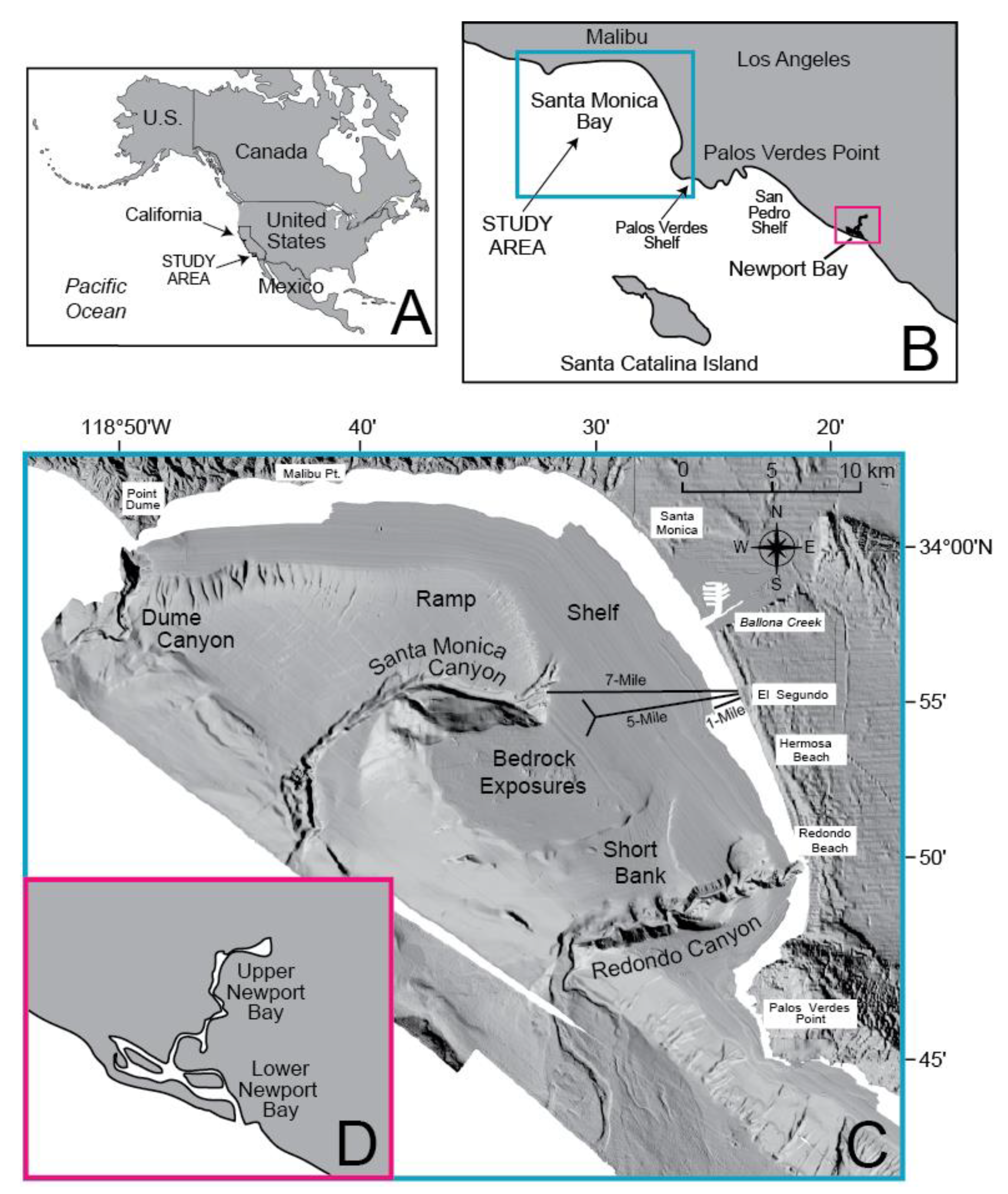
Santa Monica Bay is located on the southwestern coast of the United States near the city of Los Angeles (Figure 1A,B). The bay extends from Point Dume to Palos Verdes Point and is bordered by the Santa Monica Mountains and the Palos Verdes Hills (Figure 1C). The continental shelf of Santa Monica Bay generally ranges from 5–8 km wide, except near the center where the shelf extends ~18 km. The shelf is incised by three canyons: Dume Canyon in the north, Santa Monica Canyon in the center, and Redondo Canyon to the south. To the north, below the shelf break at ~100 m depth, is an abbreviated and steep slope referred to as the “Ramp”; to the south, the relief is less abrupt and is known as “Short Bank.” Both lead to the Santa Monica Basin to the west.
One of the largest sewage outfall systems in southern California is located in Santa Monica Bay (Figure 1C); its history has been summarized by Dojiri [64]. In 1894, the City of Los Angeles began discharging raw sewage from the Hyperion treatment plant directly into the surf zone of Santa Monica Bay. Complaints of locally fouled beaches resulted in the construction of a screening facility and a submarine outfall one mile in length in 1925. However, due to construction problems and increased effluent flow, the extent of fouled beaches expanded, so that by 1943, coastlines as much as 10 miles distant from the outfall were affected. A new treatment plant and 1-Mile outfall were constructed in 1951 (Figure 1C). Chlorinated secondary effluent was discharged through the outfall at a depth of 14 m, while the sludge was processed and made into fertilizer. Later, this fertilizer production was not considered cost-effective and the sludge was also discharged into the Bay.
In the late 1950s two new outfalls were constructed: the 7-Mile and 5-Mile outfalls (Figure 1C). From 1957–1987, the 7-Mile outfall discharged digested sludge into the Bay at a depth of 98 m directly into the head of Santa Monica Canyon. In 1960, the 5-Mile outfall became operational, discharging unchlorinated liquid effluent at a depth of 58 m from a Y-shaped diffuser. As population increased in the city of Los Angeles, a corresponding decrease in the quality of the effluent occurred. Flow gradually exceeded the ability of the plant to provide secondary treatment and by 1985, the flow reached a maximum of 415 million gallons per day. The level of discharged solid effluent peaked as well, as only about 35% of the solids were being removed at this time. Conditions improved in 1987, however, with the initiation of both a Hyperion treatment plant improvement project and a localized water conservation effort due to drought. The combination of initiating full secondary waste treatment and decreased flow to the plant dropped the total average suspended solids discharged and improved the removal efficiency of solids to >91% in 1995–1996. Today, the 5-Mile outfall is still in use and is the main effluent outfall for the Hyperion Treatment Plant. Only in emergencies is the 1-Mile outfall used to discharge chlorinated secondary effluent.
3. Materials and Methods
3.1. Field Sampling
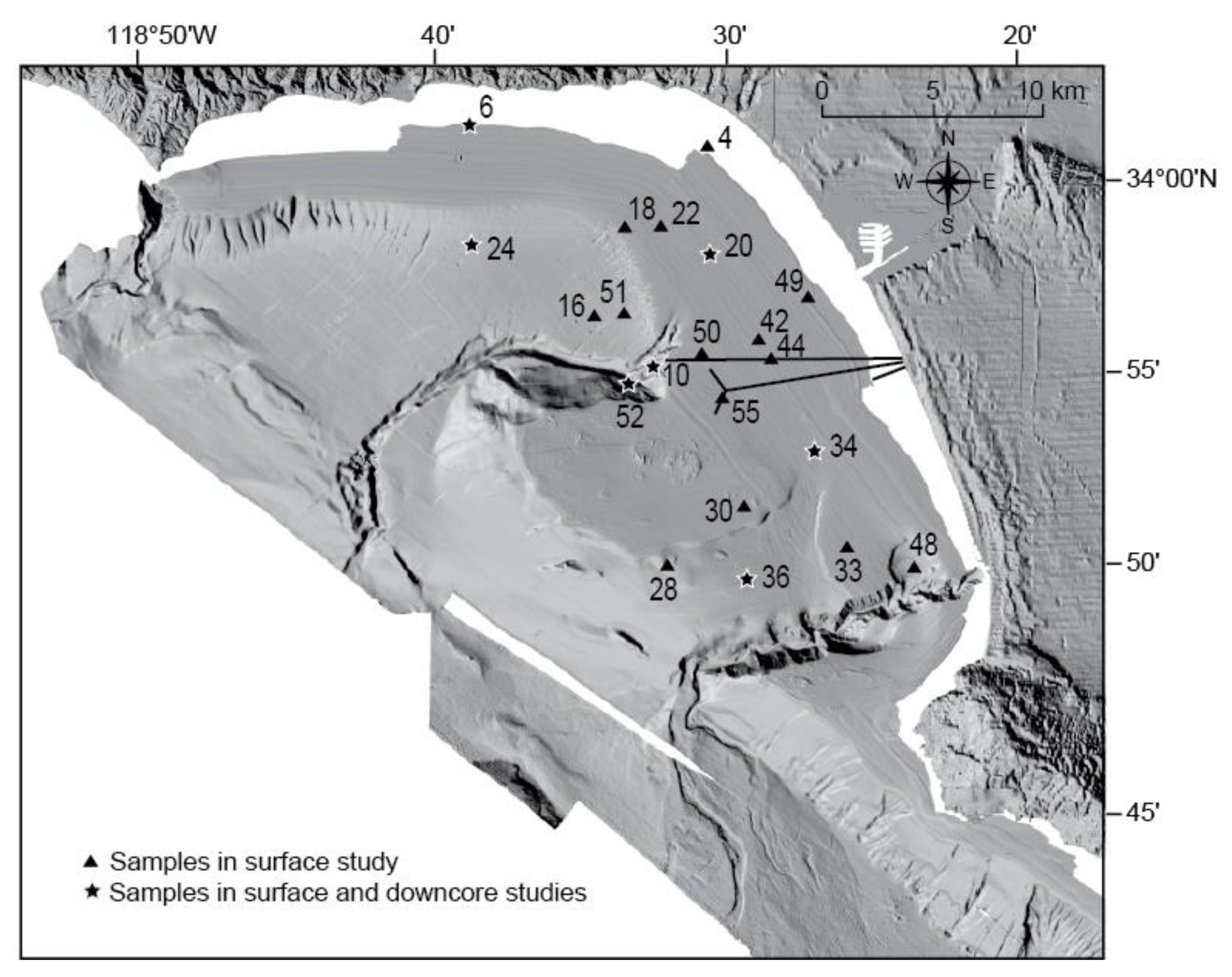
In June 1997, a standard NEL box corer on board the R/V Sproul was used to obtain sediment at 21 sites selected in a stratified random design [5] on the shelf and slope of Santa Monica Bay for geological, geochemical, and biological studies (Figure 2; Table 1). The box core had a surface area of 20 by 30 cm and a maximum depth of penetration of 60 cm. Subsamples of the upper 0–1 cm and 0–2 cm intervals were taken and preserved for microfaunal and textural analysis, respectively. Four subcores, each consisting of a plastic tube with an 8.4-cm inside diameter, were also taken from the box cores for geochemistry, toxicity, geochronology, and stratigraphy. Each tube contained a piston that was firmly attached to the sub-sampling rig that maintained the sediment surface so that virtually no core shortening occurred and the proper sub-bottom depth reference in each subcore was preserved. The tubes were driven into the intact box core at a constant speed with an electric-powered actuator. A polycarbonate liner was used for the geochemistry and toxicity subcores; the former were then frozen at −30 °C and the latter were refrigerated. A polybutyrate liner was used for both the stratigraphy and geochronology subcores. Two-centimeter-long sections of the geochronology subcores were extruded on board ship, bagged, and sent to Skidaway Institute of Oceanography for Pb-210, Cs-137, and Th-234 dating to determine sediment accretion rates and rates of biological mixing [65,66].
3.2. Chronology
Eighty sediment samples from Santa Monica Bay were prepared for radiochemical analysis at the Skidaway Institute of Oceanography [65] following standard techniques described in Alexander et al. [66]. Sediment samples for Pb-210 dating were ground into a powder, let to equilibrate for 20 days in sealed jars, and then counted for approximately 24 h. Total Pb-210 activities were directly determined by measuring the 45.5-KeV gamma peak using ORTEC (Oak Ridge, TN, USA) LO-AX germanium detectors. Supported levels of Pb-210 from Ra-226 were determined by measuring the gamma activity of Pb-214 (295 and 352 KeV) and of Bi-214 (609 KeV), the short-lived daughter products of Ra-226. Lead-210 has a half-life of 22.3 years, thereby providing a steady-state chronology [67] for the past ca. 100 years [65,68]. Accretion rates for bulk sediment were calculated from the least- squares regression of the downcore excess PB-210 activity data for each core using the mass flux rate, which accounts for changes in porosity that can affect the vertical accretion rates [65].
Caesium-137 is a transient tracer [67] resulting from atmospheric nuclear testing and has a half-life of 30.0 years [65,68]. Chronologic markers using this isotope include: (1) the onset of the Cs-137 record in 1954 due to initial bomb fallout; (2) the first fallout peak in 1959; and (3) another peak in 1963 after which input declined when atmospheric testing was banned [67,69]. A later peak was recorded in some locations due to the Chernobyl accident in 1986, but it is largely absent from terrestrial deposits in North America [70]. In sediments off southern California, the peak in 1963 has now been recalibrated to 1971 [71] due to the region’s dry climate, delaying the transport of Cs-137-absorbed terrestrial deposits to the ocean. The Cs-137 record is often used to corroborate the sediment accretion rates determined by the Pb-210 profiles [67], although clarity of the peaks has become an issue in some cases over the last few decades [71] with the two peaks merging into one, becoming elongated, appearing as multiple peaks, or not being clearly defined, all most likely the result of bioturbation [72]. Large increases in sand-sized particles are also known to introduce potential error in Cs-137 profiles [71]. In this study, Cs-137 activities were determined by measurement of the 661.6-KeV gamma peak.
The naturally occurring isotope Th-234 has a short half-life of only 24 days and is instrumental in determining biological mixing rates and depths because it adheres to sinking particles in the water column and is quickly delivered to the seafloor where it is mixed into the sediment. Samples to be used for determining Th-234 activities in this study were analyzed soon after collection by drying the sediment, grounding it into powder, and counting it for 24 h in order to quantify its gamma peak at 63 KeV [65,68]. The samples were recounted four months later to quantify the supported Th-234 levels, from which the excess levels could be determined.
Several factors, such as grain size, changes in porosity, accretion rates, and, most importantly, rates and depth of mixing due to bioturbation, introduce error into the dating process so that Pb-210 accretion rates are only estimates of the true accretion rates [65,67]. In Santa Monica Bay, measured apparent accretion rates were found to be as much as twice the actual accretion rates at some locations because of deep mixing [65]. As a result, the error for individual accretion rates was estimated at approximately 10% based on the standard error of all linear regressions calculated for Pb-210, resulting in an error for the calculated ages of about 8 years [65]. Estimates of uncertainties from just south of Santa Monica Bay on the shelves off Palos Verdes Point and San Pedro (Figure 1B) report errors of sedimentary increments of 5–10 years due just to slight differences in the Pb-210 slope mean estimates, thereby shifting the age by 10–40 years [72], or as great as centennial to millennial scales for ~5 cm intervals based on molluscan assemblages [73]. Due to these inherent dating errors, only approximate calendar ages based on the average sediment accretion rates are reported in the present study.
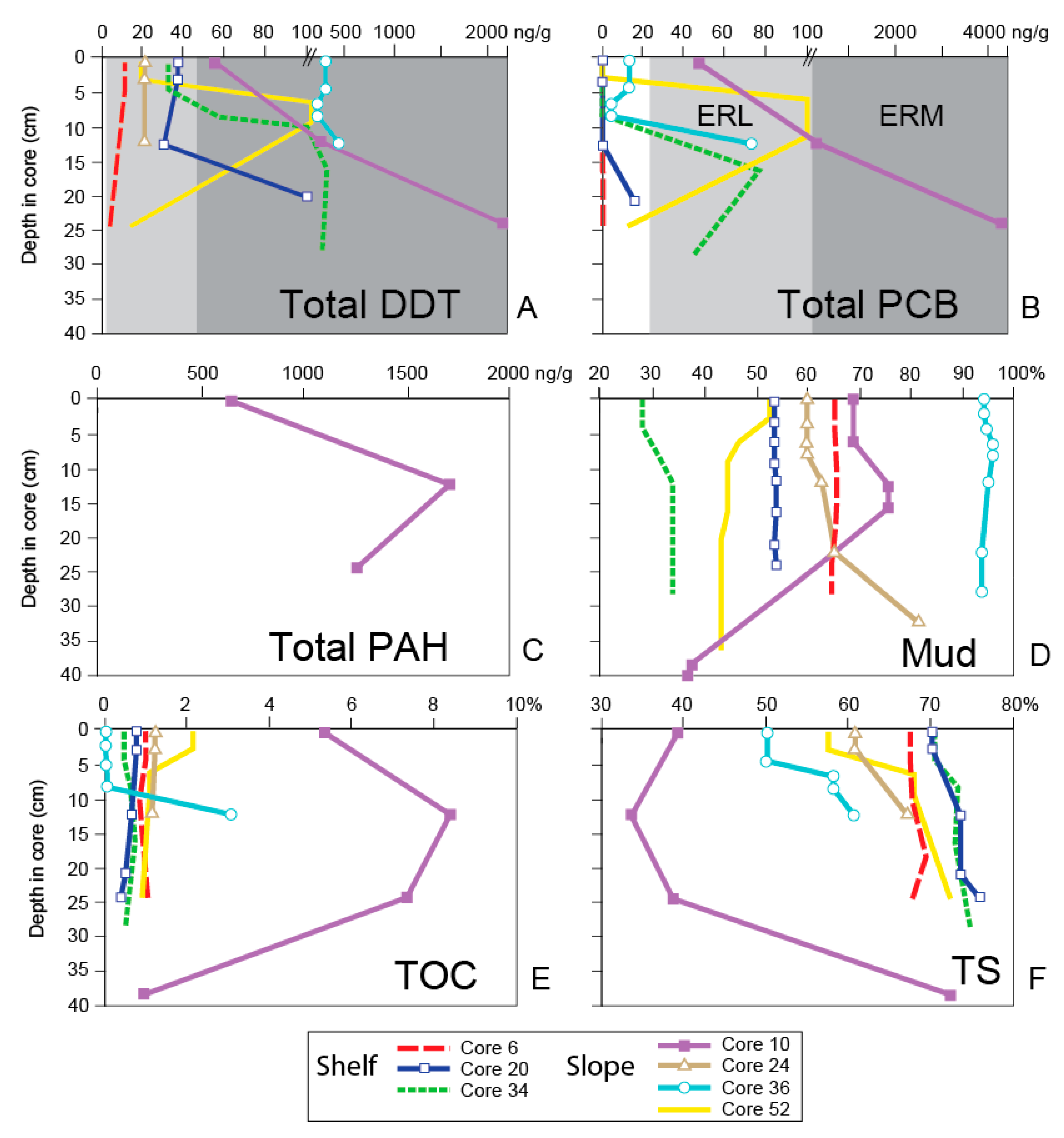
Additional factors taken into consideration in determining the chronology of the cores were peaks in Cs-137, the abundance of dichlorodiphenytrichlorethane (DDT) and polychlorinated biphenyls (PCBs), and the granulometry of the core sediments. Due to the fact that (1) the production of DDT was banned in 1970 [74], (2) input of the organic compound to the Los Angeles County Sanitation Districts sewer system ceased in 1971 [75], (3) DDT has a half-life of days [76,77] to years [78,79], and (4) it is broken down quickly as a result of dehydrochlorination by microorganisms [80], a dramatic decline was seen in DDT concentrations in Santa Monica Bay after 1979 [81]. Following a similar trend, PCBs were first manufactured in 1929 and were banned in the United States in 1979 [82], so their abundance dropped precipitously in Santa Monica Bay after 1979 as well [81]. Interestingly though, the concentration of metals has not followed this pattern, showing little temporal change since the mid-1960s, except near the 7-Mile outfall [81]. Finally, a shift from a shell-gravel substrate to one of predominantly mud on the shelves of Santa Monica Bay (investigated on Short Bank) and Palos Verdes due to siltation resulting from grazing and agriculture without concern of soil management [83] provides yet another means to date the core sediments. An epifaunal assemblage of brachiopods and scallops associated with the shell-gravel substrate persisted for thousands of years, then declined in ca. 1820–1825 AD due to the pervasive soil runoff, with the shells of those organisms ceasing to be produced by ca. 1910 [83]. Therefore, the absence of any shelly remains in the three shelf cores of this study suggests the sediment that was recovered dates to after 1910. Using these parameters, three chronological horizons of interest were identified, representing the following time periods: (1) pre-pollution (prior to ca. 1957); (2) peak pollution (ca. 1957–1987); and (3) post-pollution (after the initiation of treated discharge in 1987).
3.3. Grain Size
Grain size analysis was performed by the U.S. Geological Survey on 21 surface and 46 downcore sediment samples using 2 cm sampling intervals with a Horiba (Kyoto, Japan) Model LA-900 Laser Scattering Particle Size Distribution Analyzer [84]. Sediment samples were circulated in the sample reservoir and the particle diameters determined by detection of scattered laser light. Seventy-four different size classes between 0.88 and 1.024 µm were measured. The mean was reported for each sample and the results were converted to phi units between −1 and 9 (very coarse sand to very fine silt to clay). The percent sand, mud, and clay were also determined. Only the % mud content (i.e., the combined % silt and % clay fractions) is reported in this study. As the sampling intervals often differed slightly for the grain size and foraminiferal analyses, the mud content was estimated for the foraminiferal sample intervals using the nearest grain size determination because those values were generally consistent downcore within each core.
3.4. Foraminifera
Fifty to 100 cm3 of core top sediment (0–2 cm; “recent/present day” = 1997) was sampled at each station for foraminiferal analysis. Once the Pb-210 dating information was available [65], 50 1-cm sub-surface intervals were also analyzed for foraminifers from seven cores (Figure 2). Sediment samples were wet-sieved through nested 0.63 mm, 0.150 mm and 1.0 mm screens to segregate the size fractions. Sediment remaining on the screens was transferred to filter paper and air-dried. Foraminifera were extracted from the >0.63 mm fraction. Each sample was split with the aid of a microsplitter into an aliquot containing at least 300 benthic foraminifers, and all specimens were picked and identified. Sandy samples containing few foraminifers were subjected to sodium polytungstate flotation at a specific gravity of 2.4 g/cc in order to concentrate the foraminifers before splitting and picking. Relative foraminiferal species abundances were computed using a sum of total benthic foraminifera and converted to frequency data. The slides and residues of this study are on file at the Pacific Coastal and Marine Science Center Micropaleontology Laboratory, U.S. Geological Survey, Menlo Park, CA, USA.
3.5. Macrofaunal Toxicity Testing
The macrofaunal toxicity tests used in this study included amphipod survival and sea urchin fertilization success. Unfortunately, a broader study of bivalve community structure was not also undertaken, which would have allowed for a better comparison between the foraminiferal associations and a wider range of macrofaunal toxicity tests. Both amphipod survival and sea urchin fertilization tests used standard analytical methods [85,86] respectively and were conducted by Southern California Coastal Water Research Project (SCCWRP) personnel [5]. Juvenile amphipods of the species Grandidierella japonica Stephensen were collected from nearby Upper Newport Bay (Figure 1B,D) less than one week prior to testing. Each core was sliced into a 6-cm section (0–6 cm), and 4-cm sections thereafter. Twenty amphipods were added to a homogenized sediment-water mixture from each section and were removed by screening after ten days. Sediment was considered toxic if less than 80% of the controls survived, a standard used in other studies [87,88].
The sea urchin fertilization test used sperm and eggs of the purple sea urchin Stronglyocentrotus purpuratus (Stimpson) collected from the intertidal zone in northern Santa Monica Bay (Figure 1B,C) and water from the sediment water-interface of the amphipod survival test on the first day of the amphipod exposure. Sperm were first subjected to 20 min of exposure to this water. Eggs were then added and left for 20 min, allowing fertilization to proceed. The eggs were removed, preserved, and later examined with the aid of a microscope to determine if fertilization occurred. Sediments were considered toxic to sea urchins if the mean fertilization was significantly lower (p < 0.05; less than 80%) than the controls. Amphipod survival and sea urchin fertilization results presented as greater than 100% indicate that the animals did better in the sediment than in the controls.
3.6. Chemical Analysis
Cores were stored frozen at −20 °C until the metals, organic compounds, and total organic carbon (TOC) (together, referred to as Potential Toxic Elements in Martínez-Colón et al. [17,18,19] were analyzed by staff at SCCWRP [79]. The cores were then allowed to thaw, and sub-sampled with a piece of beveled glass into 1 or 2 cm sections at the desired depths based on the Pb-210-dated horizons. Trace metals analyzed included arsenic, beryllium, cadmium, chromium, copper, lead, mercury, nickel, silver, zinc, and iron; other sediment constituents included unionized ammonia (toxicity is thought to be primarily attributable to this form, NH3, compared to ionized ammonia, NH4) and percent total solids; and organics included total DDT, total PCBs, and total polycyclic aromatic hydrocarbons (total PAHs). The analyses were conducted as described in Bay et al. [81].
Each sediment sample to be measured for metals was digested using Method 3055 of the United States Environmental Protection Agency SW-846 protocols (third edition), and eventually analyzed using Method 6010 of the U.S. EPA SW-846 protocols. Some metals expected to have low concentrations were analyzed with graphite furnace atomic absorption spectroscopy (U.S. EPA Method 7010), and mercury was analyzed with a cold vapor method (U.S. EPA Method 7471).
Samples to be measured for organics were extracted using a microwave-assisted solvent extractor (MSP 1000 Microwave Sample Preparation System; CEM Corporation, Matthews, NC, USA). Total DDT components and PCB congeners were measured using an HP 5890 II GC equipped with a 63Ni electron capture detector (ECD) and a 60 m 0.25 μm I.D. (0.25 mm film thickness) DB-5 silica fused capillary column (J&W Scientific, Folsom, CA, USA). Total PAHs were measured using an HP 5890 II GC equipped with a 5970 mass spectrometer (MS) and a 60 m 0.25 mm I.D. (0.25 μm film thickness) DB-5 silica fused capillary column (J&W Scientific, Folsom, CA, USA).
Sediment TOC was obtained from the difference between the measured concentrations of total carbon and total inorganic carbon, the latter of which were analyzed on a carbon dioxide coulometer (System Model 5010; UIC, Inc., Fremont, CA, USA).
3.7. Data Analysis
A Spearman rank-order correlation using Aabel (v.3), a statistical software package created by Gigawiz Ltd. Co. (Tulsa, OK, USA), was used to analyze the foraminiferal abundances of B. denudata and E. advenus, as well as the toxicity and chemistry data, to determine any associations that might exist between them. This nonparametric correlation was applied to the biotic (percentage abundances of benthic foraminifera, sea urchin fertilization success, and amphipod survival) and abiotic (environmental) data, the latter comprised of sediment concentrations of trace metals and organics as well as TOC, total solids (% TS), mud content (%), and unionized ammonia. When the biotic data, % TS and % mud were correlated among themselves, the variables were not transformed because they were all expressed in similar units (percentage abundance) and none of these were rare so there was no need to down-weight the importance of the highly abundant constituents [89]. In contrast, the abiotic data were measured on different scales, warranting a log transformation followed by normalization [89,90,91]. Both biotic and abiotic correlations were interpreted at the p < 0.05 confidence level. Species abundance, toxicity, and chemistry data were also compared using effects range-low (ERL) and effects range-median (ERM) values; the ERL and ERM concentrations are the concentrations above which adverse biological effects are possible (10%) and probable (50%) for organisms living in the sediment, respectively [92].
Sediment concentrations in this study are occasionally presented as less than a threshold instead of an actual number (Appendix A). For example, in the case of silver, the concentration is reported in 39 samples as <2.6 µg/g, making it impossible to determine exceedances above the ERL of 1.0 µg/g (Table 2). As a result, the abundance of silver was not plotted in respect to ERL or ERM concentrations in the cores, nor included in the Spearman correlation. For three other sediment chemistry analytes (<17 µg/g of copper in 29 samples, <0.42 µg/g of cadmium in four samples, and <0.04 µg/g of mercury in one sample), the concentrations did not affect determinations of any ERL or ERM exceedances, so these were plotted downcore but were eliminated from the Spearman correlation.
4. Results
Of the seven cores collected in this study, average sediment accretion rates ranged from 0.31 to 0.52 cm/year on the shelf and 0.19 to 0.49 cm/year on the slope (Figure 3; [65]). The locations with the highest accretion rates were Core 6 (0.52 cm/year) off Malibu Point and Core 10 (0.49 cm/year) near the 7-Mile outfall (Figure 2). Based on the Pb-210 profiles and, where available, penetration depths of excess Th-234, the SML ranged in depth from <1.5 cm to 23 cm, with the deepest mixed layers occurring in cores 6 and 34 from the shelf. Calendar ages based on the Pb-210 accretion rates suggest that most of the cores date back to the early 1900s, and the lack of shell-gravel sediment at the bottom of the three shelf cores also indicates they are younger than ca. 1910 [83]. However, two cores (36 and 52) obtained on the slope may have captured the latter portion of the 19th Century, although the Cs-137 record of Core 36, as well as the persistence of PCBs downcore in Core 52, suggests they may be younger. The chronologies are supported by the depths of the SML, as the effective resolution of the sampled intervals (the SML/accretion rate) compares well with the calendar years assigned to the upper portion of each core. Most cores also displayed two or more peaks in Cs-137.
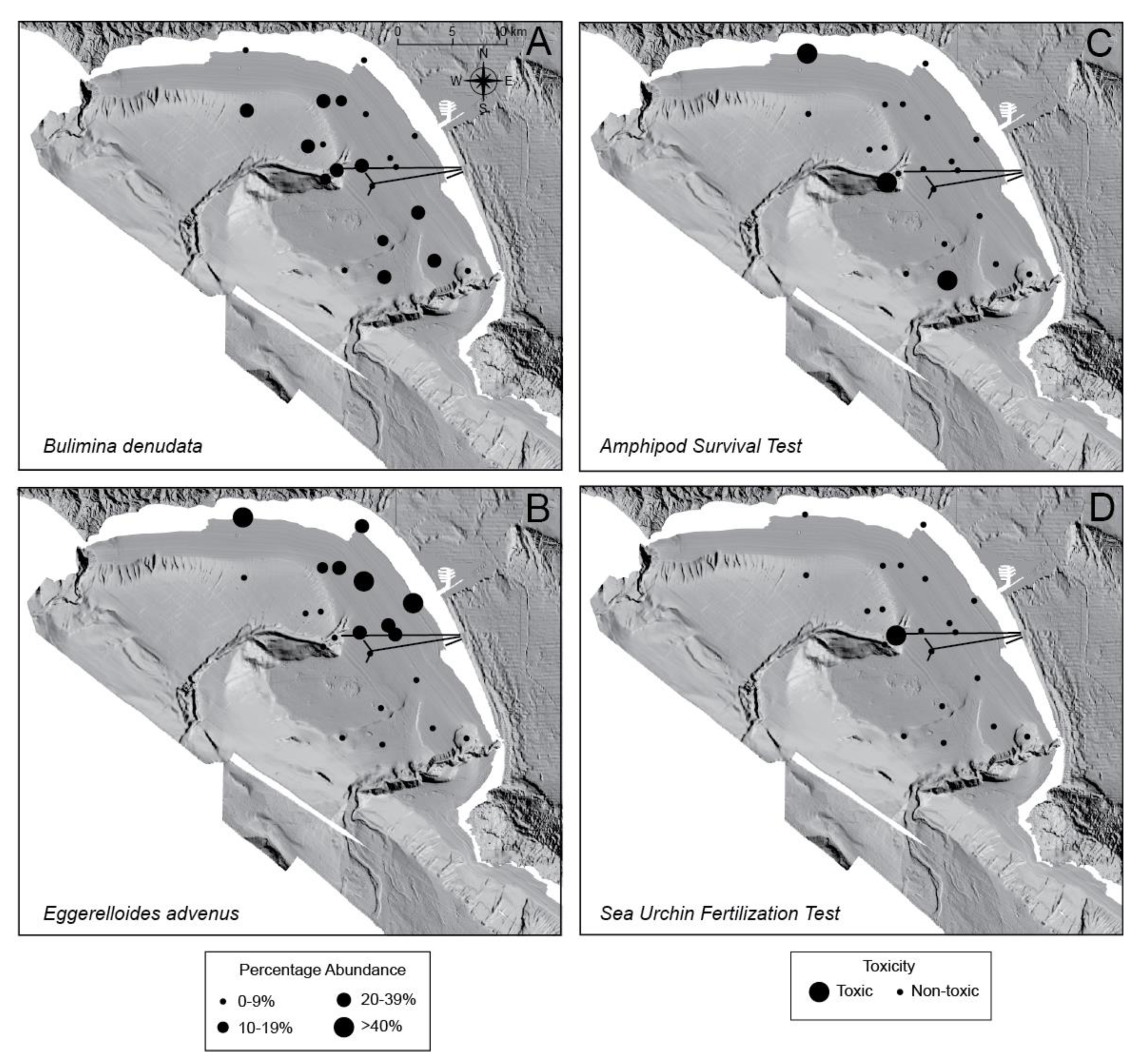
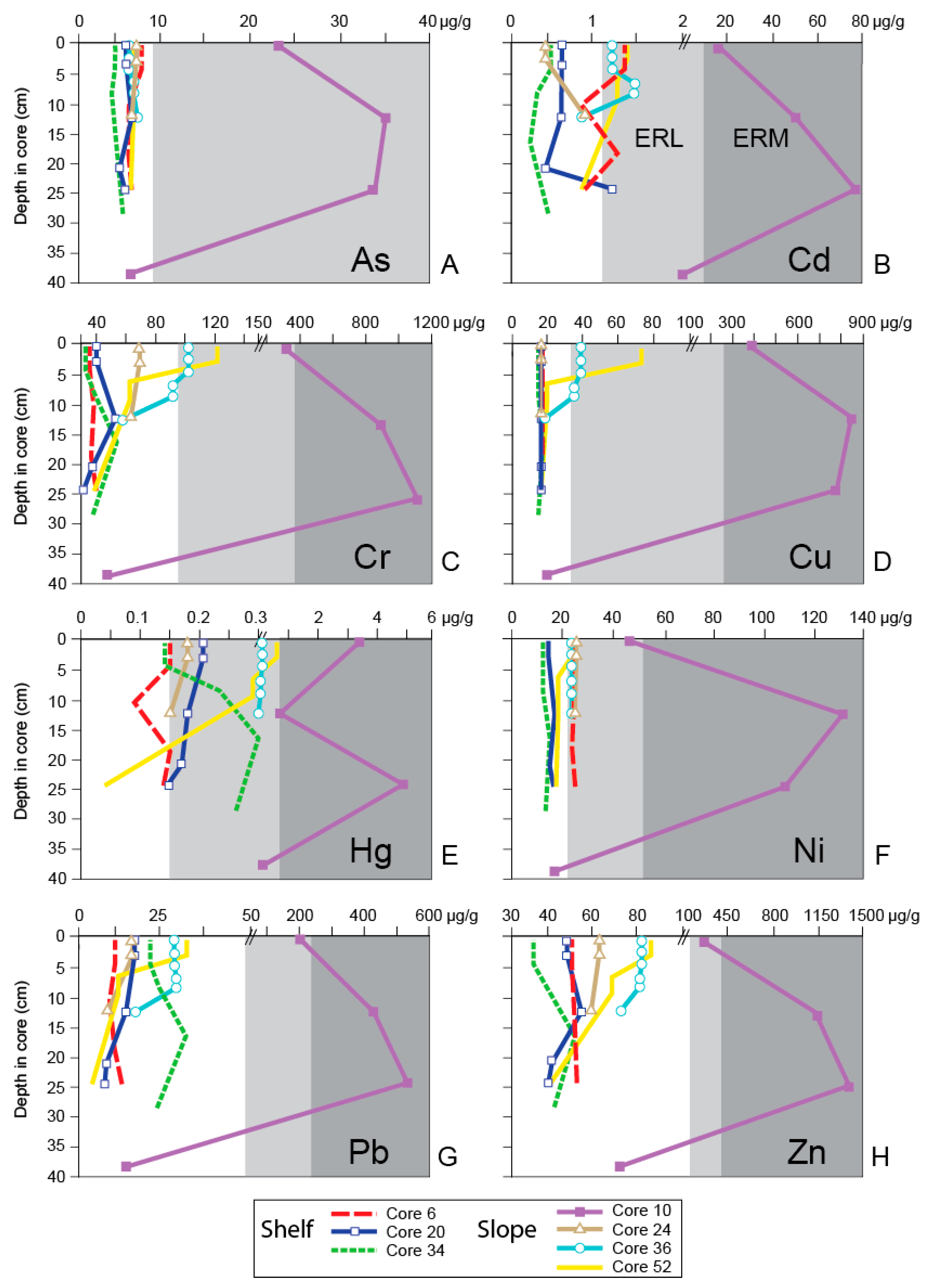
Bulimina denudata averaged 16% of the foraminiferal assemblage of the 21 surface samples analyzed (Figure 4A). Eggerelloides advenus was locally more abundant and the species’ abundance only slightly higher on average (18%; Figure 4B). The amphipod survival test identified only three of 21 surface samples as being toxic (Cores 6, 36, and 52; Figure 4C; Appendix A), with survival rates of 68, 38 and 74%, respectively, whereas the sea urchin fertilization test indicated that the surface of only Core 10 was toxic (28% fertilization success; Figure 4D; Appendix A). The ERM values were exceeded for the trace metals cadmium, copper, mercury, and silver, and trace organics (total DDT and total PAHs) in Core 10; for silver in Cores 16, 51 and 52; and for DDT in Cores 28, 30, 33, 36, and 48 (Figure 5 and Figure 6) [83]. The ERL values were exceeded in two cores for arsenic, seven for cadmium, six for chromium, four for copper, one for lead, eleven for mercury, seven for nickel, one for zinc, 15 for total DDT, and one for total PCBs.
The abundance of B. denudata in the 48 downcore samples was higher in most cases than in the surface samples (18%) whereas E. advenus was less abundant (averaging 10%) except for near-recent samples in Cores 6 (4–5 cm, 66%) and 20 (2.5–3.5 cm; 53%) (Figure 7A–G; Appendix A). The amphipod survival test suggests far more downcore samples were toxic compared to the surface material (21 versus 3), yet the sea urchin fertilization test only identified the five samples from Core 10 as toxic. The ERM values were exceeded for nearly all metals in Core 10 (cadmium, chromium, copper, lead, mercury, nickel, silver, and zinc), as well as total DDT and total PCBs. The ERM value for total DDT was also exceeded in Cores 20, 34, 36, and 52. The ERL values were exceeded in a minimum of three cores for cadmium, chromium, mercury, nickel, total DDT, and total PCBs, two for copper, and one for arsenic.
In all samples (surface and downcore), a weak but significant positive correlation was found between the abundance of B. denudata and both amphipod survival (rs = 0.263; Table 3) and total DDT (rs = 0.294; Table 4). A weak but significant negative correlation was evident between the abundance of E. advenus and sea urchin fertilization success (rs = −0.252; Table 3) and the abundance of B. denudata and arsenic, cadmium, unionized ammonia, and TOC (rs = −0.289 to −0.326, Table 4). Nine sediment constituents significantly correlated with the abundance of E. advenus, eight were weakly to moderately negatively correlated (arsenic, beryllium, chromium, copper, nickel, zinc, iron, TOC, and total DDT; rs = −0.285 to −0.558) and unionized ammonia was moderately positively correlated (rs = 0.357). When only the surface samples were analyzed, no significant correlations were found between any sediment constituent and the abundance of B. denudata, or between the abundance of either species versus amphipod survival and sea urchin fertilization. In contrast, a moderate to strong negative correlation was evident for eight trace metals (arsenic, beryllium, chromium, lead, mercury, nickel, zinc, and iron) and TOC with the abundance of E. advenus (rs = −0.438 to −0.832) as well as a strong positive correlation with percent total solids (rs = 0.611). In the downcore samples, a moderate negative correlation (rs = −0.388 to −0.560) was found between the abundance of B. denudata and arsenic, cadmium, unionized ammonia, and TOC, whereas only beryllium, cadmium, total PCBs, and sea urchin fertilization success correlated moderately negatively with the abundance of E. advenus (rs = −0.340 to −0.501).
Grain size, reported here as % mud content, is lowest on average on the outer shelf at site 50 (19%) and on the mid–shelf north of Short Bank at site 34 (32%), whereas the highest values occur west of Short Bank at site 36 (95%), at the bottom of core 24 (82% at 32–33 cm), in surface sediment at site 16 (81%), at site 10 located near the terminus of the 7-Mile outfall from a depth of 25 cm to the core top (63–76%), and at site 6 near Malibu Point (66%) (Figure 2). No correlation was found between mud content and the abundance of either B. denudata or E. advenus in the surface or downcore samples when analyzed separately, or when all of the surface and downcore samples were analyzed together (Table 4).
5. Discussion
5.1. General Trends of Toxicity in Santa Monica Bay
The sediment chemistry measurements [81] and macrofaunal (amphipod survival and sea urchin fertilization) toxicity tests [5] indicate that many surface and downcore sediment samples in Santa Monica Bay were toxic, including those dated prior to 1957–1960 when the 7-Mile and 5-Mile outfalls became operational. The most likely explanation for the presence of toxic sediments downcore is due to the downward migration of contaminants by bioturbation [5]. The spatial and temporal pattern of toxicity suggests that the historical inputs of the 7-Mile sludge outfall was the most likely source of the pollution, and that remediation has improved sediment quality and decreased the size of the impacted area, so that only a few sites in the bay were toxic when the samples were collected in 1997 [5].
In Santa Monica Bay, the amphipod survival tests identified toxic samples more often than the sea urchin fertilization tests, whereas the toxicity effect of the latter was more pronounced [5]. According to Greenstein et al. [5], amphipod survival rates negatively correlated (rs = −0.242) only with the concentration of silver in the sediment, whereas poor success with sea urchin fertilization was associated with high concentrations of zinc, silver, copper, cadmium, and total PCBs and PAHs. The high levels of DDT found throughout the bay [81] did not correlate significantly with either amphipod survival or sea urchin fertilization, possibly due in part to the fact that the amphipod used in this study (Grandidierella japonica) is tolerant of the pesticide [93], and neither did grain size [5]. These tests suggest that although both amphipods and sea urchins are sensitive to pollutants, they respond to sediment constituents in a different manner.
5.2. Temporal Trends of Toxicity in Santa Monica Bay
Seven times more downcore samples proved to be toxic according to the amphipod survival test than at the surface (Appendix A). This is due to the fact that the major source of contamination historically to Santa Monica Bay was the contaminant inputs from wastewater discharge from the Hyperion Outfall system that declined drastically during the last few decades as a result of improved treatment processes and better source control [81].
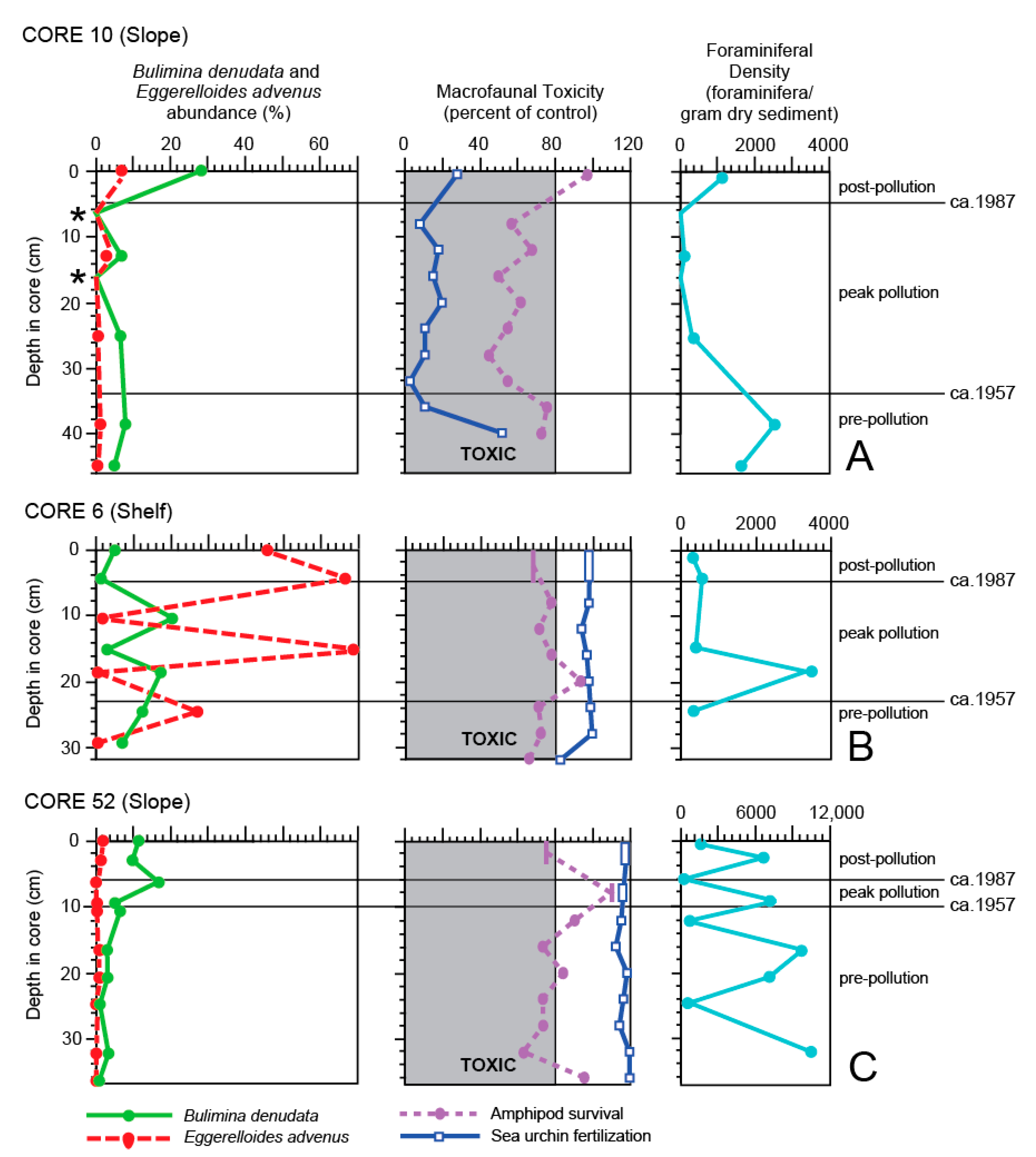
The temporal pattern of toxicity was most evident in Core 10 which was collected near the terminus of the 7-Mile outfall (Figure 2) and is the longest and most contaminated of this study. The Pb-210 profile indicates the core contains sediment dating back to the early 1900s and the SML extends down to 6.5 cm (Figure 3). However, the Cs-137 record suggests deposition starting in the middle 1900s. Unfortunately, no trace organic compounds were measured prior to 24–25 cm, but at that depth DDT and PCBs were already at ERM levels (Appendix A) and at the highest concentrations recorded in any of the cores. Therefore, the Pb-210 chronology appears to be indicating calendar ages that are too old downcore. Based on the Cs-137 peaks and the DDT and PCB values, the pre-pollution period is thought to range from the bottom of the core to ca. 34 cm, the peak pollution period from ca. 34–5 cm, and the post-pollution from ca. 5 cm to the core top.
Although both macrofaunal toxicity tests suggest the sediment was toxic during the pre-pollution period (Figure 7A), at 38–39 cm sediment chemistry values of the trace metals were low (only cadmium and mercury exceeded ERL values; Appendix A), mud content was 40%, TOC was moderately low at 0.907%, and the foraminiferal density (i.e., FD = the number of foraminifera/gram dry sediment) increased to 2511 from 1621 further downcore at 44–45 cm (Figure 7A). Together, these indicate that the concentrations of the trace metals were not, in fact, toxic to the benthic foraminifera. However, since the trace organic compounds were not analyzed at this depth in the core, they cannot be ruled out as being responsible for the macrofaunal toxicity results.
From 1960 to 1987, the 7-Mile outfall discharged untreated effluent and roughly 7x10⁹ L of sludge annually, and even larger amounts from 1982–1987 due to reduced levels of treatment because of decreased efficiency of plant operations [94]. As a result, the % total solids decreased by nearly one half (Figure 6) and the sediment accretion rate at the core site which averaged 0.49 cm/year below the SML (Figure 3) is reported to have been as high as 2.28 cm/year adjacent to the 7-Mile outfall [81]. Foraminifers were extremely rare during this peak pollution period, particularly at 6–7 cm and 15.5–16.5 cm when the site nearly became a dead zone. At 24–25 cm, all of the trace organic compounds and nearly all of the trace metals exceeded ERM levels, both amphipod survival or sea urchin fertilization toxicity tests identified the sediments as contaminated, mud content rose to 63%, TOC increased dramatically to 7.3%, and the FD dropped significantly to 379 (Figure 5, Figure 6 and Figure 7).
Most chemical constituents continued to exceed ERM levels at the latter stages of the peak pollution period. These exceedances are not surprising with the continued outfall discharges and the mud content reaching a peak of 76% at this time, as fine-grained sediments are known to adsorb heavy metals and organic compounds [95,96,97]. At 12–13 cm, total organic carbon increased to the highest concentration of any sample in this study (8.4%) and the FD continued to decline (to 141). The amphipod survival and B. denudata abundance curves were similar with depressed values, as were the sea urchin fertilization success and abundance of E. advenus (Figure 7A).
Site 10 was the only surface site (0–2 cm) considered toxic based on the sea urchin fertilization test, as well as being the most contaminated of the surface sites based on sediment chemistry, exceeding ERM values for cadmium, copper, mercury, silver, total DDT, and total PAHs, and ERL levels for arsenic, chromium, lead, nickel, zinc, and total PCBs (Figure 5 and Figure 6). However, the FD increased by nearly 1000 (1126; Figure 7A) as the mud content decreased to 69% and the TOC value, although still very high, decreased to 5%. The high FD possibly reflects the ability of foraminifera to use organic waste as a food source [10,29,57]. The abundance of B. denudata (28%) also increased by a factor of four over its abundance at 12–13 cm, exceeding its average of 16% for all of the surface samples (Appendix A), and again, possibly demonstrating the species’ propensity for settings with high food availability and low oxygen [56,57,58]. In contrast, the abundance of E. advenus did not change dramatically from that at 12–13 cm (3% to 7%), compared to an average of 18% for all of the surface sites, and its abundance negatively correlated with most trace metals, TOC, and % TS in the surface samples (Table 4).
The second most contaminated site was 6 (Figure 2), located far north of the 7-Mile or 5-Mile outfall sites. The core was collected on the shelf near Malibu Point, where sediment is introduced by Malibu Creek [91], one of the three sources (the others being Ballona Creek and the Hyperion outfalls) of fine-grained particulate material to the margin of Santa Monica Bay [98,99]. As a result, the mud content of the core averaged 66% and the average sediment accretion rate was the highest of any cores of this study (0.52 cm/year) [65]. The Pb-210 profile suggests the core contains a record of deposition beginning in the middle 1900s, much of which was highly bioturbated, with the SML reaching a depth of 23 cm (Figure 3). This is supported by the Cs-137 record which indicates deep mixing because the values never reached zero downcore. Despite this, Cs-137 peaks in the 1950s and ca. 1971 were observed, similar to those seen in Core 10. The deepest sample analyzed for organic compounds was at 24–25 cm and DDT was recovered at the ERL level, suggesting toxic sediment was already being deposited. Combined, the pre-pollution period appears to be from 29–23 cm, the peak pollution period from 23 to 5 cm., and the post-pollution period from 5–0 cm.
According to the amphipod survival test, sediment from Core 6 was toxic for most of the length of the core, including the core top (Figure 7B), even though no ERM values were exceeded (Figure 5 and Figure 6; Appendix A). However, ERL values were surpassed at many sub-surface levels and in the surface sediment for cadmium, mercury, nickel and total DDT; no PCBs were recovered. Throughout the core, the abundance of TOC was moderately low (0.858–1.065; Appendix A) and the FD remained low (288–528, average 375). The exception was the sample from 18–19 cm in which amphipod survival was no longer toxic (94%), the FD increased by a factor of ~10 (to 3358), and the abundance of B. denudata was one of the highest in the core (17%). These factors possibly suggest a short-term improvement in sediment quality, although some sediment chemistry data are missing (i.e., TOC and total organic compounds) which hinders an explanation. The curves for amphipod survival and the abundance of B. denudata do not track each other as well in this core as in some of the others, particularly from ca. 15 cm and above (Figure 7B). This is also the only core in which the abundance of E. advenus comprised a dominating >65% of the assemblage at two intervals: from 14.5–15.5 cm during the peak pollution period and at 4–5 cm after remediation began. In both instances, the abundance of B. denudata dropped to <5%. The poor tracking of B. denudata abundance with amphipod survival and dominance by E. advenus over B. denudata are not consistent with the other cores in this study and likely reflect the significant sediment mixing occurring throughout most of the core. However, the spikes in abundance of E. advenus may also reflect the species’ ability to quickly colonize formerly impacted areas [50,63]. Interestingly, the sea urchin fertilization success showed little change and indicated no toxicity throughout the core.
Core 52, obtained on the slope near Core 10 in the vicinity of the 7-Mile outfall terminus (Figure 2) contains a sediment record going back to the late 19th Century according to the Pb-210 profile (Figure 3), with an average sediment accretion rate of 0.25 cm/year [65] and an SML at the shallowest of any core (<1.5 cm). Peaks in the Cs-137 record occur in the upper half of the core, thereby indicating the latter half of the 1900s, although they are not as well defined as in other cores. Unfortunately, trace organics were not measured at every horizon in this core, yet PCBs are present at 24–25 cm, suggesting the sediment is at least from >1929 at that depth. The dramatic increase in DDT and PCBs to ERM and ERL levels, respectively, from 10–6 cm suggests this interval represents the peak pollution period. The core is characterized by sediment exceeding ERM values for silver and total DDT, as well as surpassing ERL values for cadmium, copper, chromium, nickel, and total PCBs downcore (Figure 5 and Figure 6; Appendix A). The only change from this pattern in the core top sediment was a slight reduction in the amount of total DDT, where it exceeded only the ERL level (Figure 6A). The mud content steadily increased from 44% at the bottom of the core (36–37 cm) to 53% at the top, as did the TOC (0.9% to 2.14%), reflecting increased input from the outfall, although the average sediment accretion rate for the core did not change significantly after the outfalls became active.
The amphipod survival test showed evidence of toxicity for most of the lower half of Core 52 and at the top of the core as well (Figure 7C). Similarities were seen between the amphipod survival and B. denudata curves, with both reaching peak abundances near the top of the peak pollution period at 6–7 cm (108% and 16%, respectively) and then declining toward the top of the core during the post pollution period (74% and 11%). Only the bottom of the core showed opposite trends, a pattern which cannot be explained at this time. The sea urchin fertilization success and the abundance of E. advenus exhibited reverse patterns, as the former exceeded the success of the controls, but the latter made up only a small proportion of the foraminiferal assemblage throughout the core (0–2%). Foraminiferal density fluctuated between extremely high (6878–10,775) and lower (537–981) values in the core, yet displayed a general trend of decreasing upcore, eventually with a FD = 1903 at the core top. This pattern did not coincide with an obvious change in macrofaunal or sediment chemistry toxicity and also cannot be explained at this time.
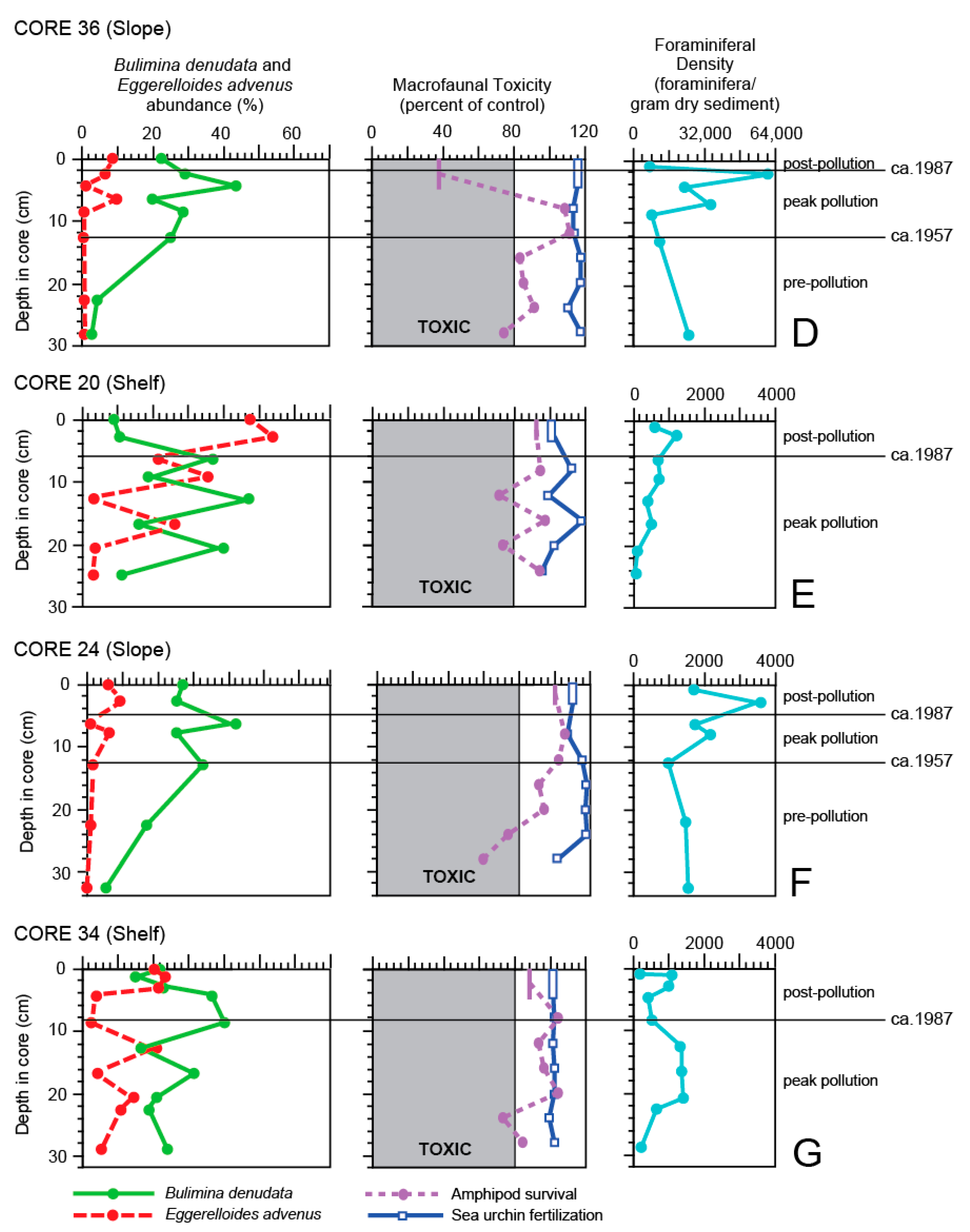
Core 36 was collected in the southern portion of Santa Monica Bay on Short Bank (Figure 2), far from the outfalls and at a depth of 125 m. As with Core 52, it contains late 19th Century deposits based on the Pb-210 record, although the Cs-137 record suggests the early 1900s instead. This site had the highest mud content (95%) and lowest average sediment accretion rate (0.19 cm/year; Figure 3) [65] of any in this study. The lower boundary of the SML, based on the Pb-210 and Th-234 records, was fairly shallow at 3.5 cm. However, multiple peaks are seen in the Cs-137 profile and values never reached zero downcore, suggesting both surficial and deep mixing in this core. An offset is also evident in the Pb-210 and Cs-137 records at ca. 20 cm, which marks a change in deposition. With missing chemical constituent data for the lower portion of the core, the estimate of the pollution boundaries are difficult; it is suggested that the onset of the peak pollution period coincides with the first (and already extreme) occurrence of DDT and PCBs at 12–13 cm, just below the 1959 Cs-137 peak, and continues up to 2 cm.
The ERM values were exceeded for total DDT for all sediment chemistry samples from the 13 cm to the core top, whereas ERL values were exceeded for cadmium, chromium, copper, nickel and total PCBs at many levels (Figure 5 and Figure 6; Appendix A). The DDT may have been transported to the core site by prevailing currents that flow toward the northwest along the shelf and upper slope [100] from the Palos Verdes margin where a large DDT deposit is located [101].
Generally, the amphipod survival and B. denudata curves are similar for Core 36 (Figure 7D), except for the addition of two foraminiferal samples at 6.5–7 cm and 4–5 cm where amphipod survival data were not available. The amphipod toxicity data identified the core top and lowermost (27–29 cm) sediment as toxic, and B. denudata abundances also declined there. Abundance of E. advenus was low throughout most of the core (<0.5–2%), only increasing to a maximum of 10% at 6.5–7 cm and 8% in the core top when B. denudata declined. Additionally, as with Core 52, E. advenus showed an opposite trend from the sea urchin fertilization success, which surpassed the controls for the entire core. This site had, by far, the highest FD (8047–63,127) of any core of this study, despite the fact that TOC was low from 8–9 cm on (0.062–0.017%) (Figure 7D; Appendix A). The extremely high FDs are attributed to a slow sediment accretion rate at the site. Although not quite as high, a FD = 26,258 was reported in the southwestern margin of Biscayne Bay, Florida, a region thought to be influenced by reduced salinity and elevated organic-carbon concentrations [102].
Core 20, obtained on the mid-shelf (Figure 2), features a Pb-210 profile suggesting a sediment record back to the early 1900s with an average sediment accretion rate of 0.31 cm/year (Figure 3) [65], although the Cs-137 profile indicates only sediments from the middle 1900s were deposited (Figure 3). The Pb-210 and Th-234 records indicate the SML is from 0–5.5 cm. As DDT and PCBs occur at high concentrations near the bottom of the core (20–22 cm), most of the core is considered to represent the peak pollution period. The boundary with the post-pollution periods is taken to be at ca. 6 cm based on foraminiferal and macrofaunal toxicity data.
Site 20 was most affected by total DDT, exceeding ERM values once downcore and at all other levels for ERL values (Figure 5 and Figure 6; Appendix A). Otherwise, ERL values were exceeded only rarely for cadmium and mercury. As the average sediment accretion rate for this was not as high as those found at several other sites, especially those near the outfall, the low FD values (81–572, averaging 313; Figure 7E) from 25–12 cm indicate stressed environmental conditions existed in the peak pollution period.
A saw-toothed pattern of both amphipod survival and success of sea urchin fertilization is evident in Core 20 (Figure 7E), with amphipod survival also indicating sediment toxicity at 20–22 cm and 12–13 cm, and sea urchin fertilization indicating only non-toxic sediment. This unique pattern is also seen in the abundance of E. advenus, with peaks in abundance alternating with B. denudata. This is the only other core besides Core 6 in which the abundance of B. denudata does not generally follow that of amphipod survival; the saw-tooth pattern is present but is offset slightly downcore. However, because (1) every effort was made to disturb the sediment as little as possible during box coring and subsequent sub-coring, (2) the Pb-210 and Th-234 records indicate the SML did not extend through most of the length of the core like Core 6 but was restricted to the upper 5.5 cm, (3) no unique array of contaminants were found at this site, and (4) the abundance of B. denudata and amphipod survival has tracked fairly well in all other cores, another factor may be responsible for the offset pattern. That is, it may be due to the presence of unseen gently dipping beds in the box core that resulted in the sediment of the two subcores (for foraminiferal analysis and macrofaunal toxicity) actually being non-contemporaneous when sampled at the same depth downcore.
Core 24 was obtained on the northern portion of the Ramp (Figure 2) and had an average sediment accretion rate of 0.43 cm/year (Figure 3) [65]. Based on the Pb-210 and Th-234 values, the SML extended to 4.5 cm. The Cs-137 profile is not well defined in the core and few samples were measured for sediment constituents, making the depositional history difficult to interpret. Based on the presence of DDT at ERL levels at 12–13 cm, the pre-pollution period is thought to range from 33 to 12.5 cm, the peak pollution period from 12.5–5 cm, and the post-pollution period from 5–0 cm.
The only sediment chemistry constituents to exceed ERL values in Core 24 were nickel and total DDT (Figure 5 and Figure 6; Appendix A). Except for an anomalously low value from 7.5–8.5 cm, the curves of B. denudata abundance and amphipod survival were similar, whereas the abundance of E. advenus was opposite that of B. denudata (Figure 7F). The amphipod survival test suggested sediment quality was poor prior to the 1950s, although the FD did not indicate this with values in the 1400s. Bulimina denudata abundances were also low at this time, reached a maximum during the peak pollution period (at 6–7 cm), and then declined after remediation was undertaken in 1987. The FD value was the highest (3422) for this core at 2.5–3.5 cm, indicating a return to non-impacted conditions after remediation.
Core 34 was obtained on the shelf near Short Bank (Figure 2). This core was similar to the other shelf cores by having an average sediment accretion rate of 0.32 cm/year like Core 20 [65] and having a substantial SML like Core 6, but here it only reached a depth of 17 cm downcore instead of 23 cm (Figure 3). The Pb-210 profile suggests the record goes back to the early 1900s, but the Cs-137 record indicates only the middle 1950s. The latter is supported by the occurrence of PCBs at an ERL level at the bottom of the core (28–29 cm), making the age > 1929. Maximum concentrations of DDT and PCBs occur from the bottom of the core to 16–17 cm, suggestive of the peak pollution period with no pre-pollution period represented. This coincides with the second Cs-137 peak, interpreted as 1971. No PCBs were recovered from 8–9 cm to the core top and DDT values also decreased, marking the post-pollution period (9–0 cm).
Only one sediment sample (22–23 cm; Appendix A) in Core 34 was contaminated according to the amphipod survival test. Except for total DDT, ERL values were exceeded only for mercury and total PCBs at two levels (Figure 5 and Figure 6). The Total DDT concentration exceeded ERL values in the upper 5 cm of the core and ERM levels for the remainder of the core. The abundance curves of B. denudata and E. advenus are opposite one another, with B. denudata maxima at 8–9 cm and 4–5 cm (Figure 7G). Like that seen in Cores 6 and 20 also from the shelf, this pattern of alternating dominance by B. denudata and E. advenus, particularly upcore from 17 cm, coincides with the position of the SML and may reflect bioturbation. The amphipod survival and B. denudata abundance curves are generally similar, except for the latter’s low value at 12–13 cm, whereas sea urchin fertilization shows little change throughout the length of the core. The FD is generally ≤1000 in the core except for particularly low values at the bottom of the core at 28–29 cm (303), at the beginning of the post-pollution period (422–527), and especially in the 1997 core top (194).
5.3. Bulimina denudata and Eggerelloides advenus
Bulimina denudata comprised an average of 16% of the foraminiferal assemblage of the surface samples, residing most commonly on the outer shelf and upper slope (Figure 4A; Appendix A) [50]. No significant correlation was found in these samples between the abundance of B. denudata and high concentrations of any trace metals, trace organic compounds, other constituents measured, or macrofaunal toxicity (amphipod survival or sea urchin fertilization) (Table 3 and Table 4). These results are in contrast to the amphipod survival test that identified three surface sites as toxic, and the sea urchin fertilization test having identified an additional site (Appendix A). The species increased in abundance to an average of 19% of the assemblage downcore and was negatively correlated with arsenic, cadmium, unionized ammonia, and TOC. Comparison of amphipod survival and the abundance of B. denudata illustrates that they are generally in good agreement except for the unique saw-toothed pattern in Core 20 that may be due to analyzing non-contemporaneous sediments or in the regions impacted by sediment mixing in cores 6 and 34 (Figure 7B,E,F). When Core 20 was eliminated from the data set, the abundance of B. denudata downcore showed a moderately positive correlation with amphipod survival (rs = 0.350; Table 3) and arsenic, cadmium, unionized ammonia, and TOC (rs = 0.443–0.521; Table 4). As the species is presently abundant on the outer shelf and upper slope and was so prior to the addition of the major sewage outfalls [50], no point source of contamination appears to be responsible for its present spatial distribution in Santa Monica Bay (Figure 4A).
Eggerelloides advenus comprised an average of 18% of the assemblage of the surface samples and was most abundant on the shelf (Figure 4B; Appendix A) [50]. The species’ abundance strongly correlated (rs = 0.611) with total solids as well as negatively with TOC, and all of the trace metals analyzed except cadmium (rs = −0.438 to −0.832; Table 4). This species’ tolerance of cadmium is similar to that found in Chaleur Bay, New Brunswick, Canada where E. advenus was the single most abundant species in cadmium-rich tailings [63]. The abundance of E. advenus also showed no significant correlation with either amphipod survival or sea urchin fertilization success in the surface samples (Table 3). In the downcore samples, beryllium, cadmium, total PCBs (rs = −0.375 to −0.501), and sea urchin fertilization success (rs = −0.340) negatively correlated with the abundance of E. advenus. However, when Core 20 with its presumably offset sediments was removed from the analyses, only beryllium and total PCBs (rs = −0.477 to −0.552) as well as sea urchin fertilization displayed a moderate correlation (rs = −0.437), the latter even more significantly (dropping from ps = 0.021 to ps = 0.005). Although the species is presently abundant on the shelf of Santa Monica Bay, E. advenus occurred there only rarely prior to the addition of the major sewage outfalls [50]. It is assumed the species’ spatial distribution and abundance reflects its role as a pioneer colonizer of impacted areas, most likely due to the effluent that was released by the local outfalls.
5.4. Macrofaunal Toxicity Measures and Foraminiferal Abundance
Amphipods are the most common organism used to measure sediment toxicity [103,104,105,106] and the 10-day survival protocol is currently the benchmark test [107,108] because amphipods are among the most sensitive infaunal organisms to pollutants [109]. Grandidierella japonica was thought to be a valuable test species in sediment bioassays [5] because it: (1) is widespread in coastal areas [110,111,112]; (2) can tolerate wide ranging temperatures, salinity, and sediment types; (3) is sensitive to numerous contaminants [112,113,114,115]; and (4) has a relatively high tolerance to ammonia [114,115]. However, it is no longer considered for standardized testing because of concerns the species may adapt physiologically to contaminated sediments [93,116,117].
Other amphipod species are now recommended for routine use although the choice is regionally dependent due to local availability issues, lack of a reliable commercial supply, lack of physiological adaptation, or because the test species being used needs to be sensitive to the local pollutants of concern [118]. According to the standards set by the American Society for Testing and Materials [107], the U.S. Environmental Protection Agency [86], and the California Environmental Protection Agency [108], suggested test species in the U.S. are Ampelisca abdita Mills, Eohaustorius estuarius Bosworth, Rhephoxynius abronius (Barnard), and Letocheirus plumulosus Shoemaker. Most of these have been used in toxicity studies in the Southern California Bight (A. abdita [87], E. estuarius [7,119], and R. abronius [120]). However, E. estuarius has become the species of choice for southern California toxicity studies [6,7,119] because it is widely used outside the region and, therefore, allows for better data comparability.
On the East and Gulf coasts of the U.S., use of L. plumulosus is widespread in monitoring [121,122]. In Europe, several different taxa are used for sediment toxicity testing protocols as recommended by ICES, OSPAR, HELCOM, and SETAC-Europe, including the amphipods Corophium orientale Schellenberg, C. arenarium Crawford, C. multisetosum Stock, C. volutator (Pallas), Monocorophium insidiosum (Crawford), Monoporeia affinis (Linström), and Pontoporeia femorata Krøyer (see review [123]). Thus, it would be valuable to expand our investigation of the correlation between the abundance of B. denudata and amphipod survival to determine if it also applies to other amphipod species used in testing in the U.S. and elsewhere internationally, as it does to G. japonica.
Although the sea urchin fertilization test is a common marine bioassay used worldwide for environmental monitoring and regulatory testing of effluents and sediment pore waters [124], molluscan fertilization has been used in the southern California monitoring program since 2008 [6,7,125]. In this test, the normal development of embryos of the mussel Mytilus galloprovincialis Lamarck is measured using a sediment-seawater interface test following the methodology of the U.S. Environmental Protection Agency [126] and Anderson et al. [127], much in the same way sea urchin fertilization was measured. Thus, as with the different species of amphipods, one could investigate whether the abundance of B. denudata and E. advenus correlates with molluscan fertilization tests as well.
Finally, B. denudata is morphologically very similar to Bulimina marginata d’Orbigny which lives on the shelf and slope [128] in many other oceans exclusive of the Pacific [52]. As B. marginata has also been reported as a dominant species at contaminated sites [57,129], it may be true that both of these species respond in similar ways to contaminants. If, as with B. denudata, the abundance of B. marginata positively correlates with amphipod survival, then the possibility exists that the use of these species as sediment toxicity measures may be applied to pollution studies worldwide.
5.5. Use of Foraminifera as Toxicity Measures
The standard macrofaunal toxicity tests of amphipod survival, sea urchin fertilization, and molluscan embryo development success presently used are costly and burdensome laboratory analyses that must be completed shortly after the acquisition of field samples if the results are to be considered valid [130]. Recommendations for sediment holding times before the toxicity tests are initiated range from less than two weeks [131], to less than four weeks [6,7], to less than eight weeks [98,132,133]. One advantage of using foraminifera is that such a time constraint is not an issue. Although using living benthic foraminifera has been shown to be valuable in assessing the ecological status of marine ecosystems [15], samples can be stained for later analysis. In addition, foraminiferal shells are preserved in the sediment which provides a long-term record that may help define reference conditions or gauge the biotic response to polluted conditions and remediation, all of which are not possible with the standard macrofauna toxicity tests presently in use.
When comparing macrofaunal toxicity and foraminiferal abundances (such as those of B. denudata and E. advenus) as proxies of pollution, a few issues need to be considered. The standard macrofaunal toxicity tests use live organisms that interact with toxic compounds that are present in the sediment in a relatively uncomplicated manner (i.e., short-term direct exposure in a laboratory). In contrast, benthic foraminifera reside directly in the sediment for their lifetime. As a result, they may be a more sensitive measure of toxicity because they may be exposed to a higher contaminant load than the organisms being tested in the laboratory. This is especially true if the sediment is fine-grained and contains absorbed heavy metals and organic compounds that are bioavailable [17,18,19]. However, other factors that affect any complex marine ecosystem, such as variations in local temperature, oxygen content, amount of organic matter, prey availability, predation pressures, or changes in regional climate (e.g., El Niño/La Niña-Southern Oscillation or Pacific Decadal Oscillation) exert some control on foraminiferal abundances and distribution as well. For example, agglutinated taxa such as Eggerelloides have been shown to decline in abundance to near extinction in dysoxic environments whereas Bulimina spp. are tolerant of such conditions [134], so long-term records of variations in species abundance may reflect more than just the impact of anthropogenically induced toxicity. Additionally, foraminiferal shells are subject to taphonomic processes such as dissolution and bioturbation after death, resulting in time-averaging that may smooth the faunal trends [72,73] or in some cases, greatly bias the assemblage [135].
Despite the fact that the factors listed above may mask or enhance the impact of trace metals and organic compounds on the organisms, foraminifera are still extremely sensitive to their environment, are ubiquitous and easily sampled, and the preservation of their shells provide a historic record of environmental change due to anthropogenic impact. The findings of this study suggest that the abundance of B. denudata and E. advenus as sediment toxicity measures may have merit. Further investigations are recommended to see if this trend applies to other sites worldwide, other species of macrofauna that are locally available, and potentially other foraminiferal species.
6. Conclusions
The benthic foraminifera B. denudata and E. advenus are valuable taxa in pollution studies because they are tolerant of numerous trace metal and organic contaminants, and as such, are good indicator species. This study suggests that the surface and downcore abundance of B. denudata and E. advenus, as well as amphipod survival and sea urchin fertilization success, can provide a modern assessment, and historical record of change, of sediment quality due to anthropogenic inputs. The abundance of B. denudata was positively correlated with the survival success of amphipods and the abundance of E. advenus was negatively correlated with sea urchin fertilization. As B. denudata (with the related species B. marginata) and E. advenus are present nearly worldwide and often dominate assemblages, the temporal variation of their abundances may become a widespread cost- and time-effective tool for defining and monitoring areas affected by waste discharge. The outcome of this proof-of-concept study suggests that further investigation of the relationship between standard macrofaunal sediment toxicity tests (amphipod survival, sea urchin fertilization, and the development of normal mussel embryos) and the abundance of benthic foraminifera (B. denudata, E. advenus, and others yet to be identified) is warranted.
Funding
This research was funded by the Urban Ocean Project of the U.S. Geological Survey (Menlo Park, CA, USA), in association with the Southern California Coastal Water Research Project (Costa Mesa, CA, USA) and the City of Los Angeles (CA, USA).
Institutional Review Board Statement
Not applicable.
Informed Consent Statement
Not applicable.
Data Availability Statement
All data are contained within this article.
Acknowledgments
The author would like to thank the crew of the R/V Sproul for obtaining the samples used in this study and Steven Bay (SCCWRP) for valuable discussions. Particular thanks to Clark Alexander and Claudia Venherm (Skidaway Oceanographic Institute) for kindly supplying the radiochemical profiles and Thomas Lorenson (USGS) for additional discussions regarding them. Superb technical assistance was provided by Rendy Keaten (formerly USGS), and Jacquelin Letran, May Zhao, and Hai Le (formerly University of California, Berkeley). My thanks also to Scott W. Starratt and Jason A. Addison (both USGS), as well as three anonymous reviewers for extremely constructive comments which greatly improved the manuscript. Any use of trade, firm, or product names is for descriptive purposes only and does not imply endorsement by the U.S. Government.
Conflicts of Interest
The author declares no conflict of interest.
Appendix A

Table A1.
Samples (station and sample interval in cm), mud content (% mud), sea urchin fertilization success (% of control), amphipod survival (% of control), percent abundances of Bulimina denudata and Eggerelloides advenus, total solids (% TS), total organic carbon (% TOC), unionized ammonia, and sediment concentrations of trace metals and trace organic compounds in the 1997 surface and downcore Santa Monica Bay samples. Samples that were toxic based on percent sea urchin fertilization success and percent amphipod survival are in angle brackets. Sediment concentrations exceeding the ERL guidelines are in parentheses; sediment concentrations exceeding the ERM guidelines are in square brackets and bold. VR = very rare foraminifera recovered (sample not statistically valid; see Core 10), As = arsenic, Be = beryllium, Cd = cadmium, Cr = chromium, Cu = copper, Pb = lead, Hg = mercury, Ni = nickel, Ag = silver, Zn = zinc, Fe = iron, total DDT = total dichlorodiphenyltrichloroethane, total PCBs = total polychlorinated biphenyls, and total PAHs = total polycyclic aromatic hydrocarbons.
| No., Station, Sample Interval (cm) | Mud Content (%) | % Sea Urchin Fertilization | % Amphipod Survival | % Bulimina denudata | % Eggerelloides advenus | % TS | % TOC | Unionized Ammonia (mg/L) | ||||||
|---|---|---|---|---|---|---|---|---|---|---|---|---|---|---|
| (1) 4, 0–2 | 24.75 | 115 | 91 | 1 | 23 | 73.5 | 0.185 | 0.136 | ||||||
| (2) 6, 0–2 | 65.52 | 98 | <68> | 6 | 46 | 67.6 | 0.990 | 0.072 | ||||||
| (3) 6, 4–5 | 65.52 | 2 | 66 | 67.6 | 0.990 | 0.072 | ||||||||
| (4) 6, 10–11 | 65.99 | 94 | <71> | 21 | 2 | 68 | 0.858 | |||||||
| (5) 6, 14.5–15.5 | 65.99 | 97 | <78> | 3 | 69 | |||||||||
| (6) 6, 18–19 | 65.52 | 98 | 94 | 17 | <0.5 | 69.5 | 0.016 | |||||||
| (7) 6, 24–25 | 65.05 | 99 | <71> | 12 | 28 | 67.9 | 1.065 | 0.013 | ||||||
| (8) 6, 28–29 | 65.05 | 100 | <73> | 8 | 1 | |||||||||
| (9) 10, 0–2 | 69.31 | <28> | 97 | 28 | 7 | 39.1 | 5.351 | 0.020 | ||||||
| (10) 10, 6–7 | 69.31 | <8> | <57> | VR | VR | |||||||||
| (11) 10, 12–13 | 75.93 | <18> | <68> | 7 | 3 | 33.6 | 8.393 | 0.008 | ||||||
| (12) 10, 15.5–16.5 | 75.93 | <15> | <50> | VR | VR | |||||||||
| (13) 10, 24–25 | 62.68 | <11> | <55> | 7 | <0.5 | 38.7 | 7.349 | 0.041 | ||||||
| (14) 10, 38–39 | 39.94 | <52> | <73> | 8 | 1 | 72.7 | 0.907 | 0.024 | ||||||
| (15) 10, 44–45 | 35.30 | 5 | 1 | |||||||||||
| (16) 16, 0–2 | 80.97 | 102 | 82 | 32 | 2 | 50.5 | 2.616 | 0.000 | ||||||
| (17) 18, 0–2 | 26.65 | 119 | 100 | 32 | 16 | 72.7 | 0.501 | 0.104 | ||||||
| (18) 20, 0–2 | 53.69 | 100 | 92 | 8 | 47 | 70.3 | 0.771 | 0.102 | ||||||
| (19) 20, 2.5–3.5 | 53.69 | 10 | 53 | 70.3 | 0.771 | 0.102 | ||||||||
| (20) 20, 6–7 | 53.69 | 112 | 94 | 36 | 22 | |||||||||
| (21) 20, 9–10 | 54.23 | 18 | 35 | |||||||||||
| (22) 20, 12–13 | 54.23 | 99 | <71> | 47 | 3 | 73.6 | 0.653 | 0.012 | ||||||
| (23) 20, 16–17 | 53.83 | 118 | 97 | 16 | 26 | |||||||||
| (24) 20, 20–22 | 53.83 | 102 | <73> | 40 | 4 | 73.9 | 0.507 | 0.003 | ||||||
| (25) 20, 24–25 | 54.33 | 95 | 94 | 11 | 3 | 76.1 | 0.399 | 0.003 | ||||||
| (26) 22, 0–2 | 47.35 | 118 | 83 | 17 | 22 | 72.6 | 0.649 | 0.028 | ||||||
| (27) 24, 0–2 | 60.29 | 111 | 100 | 27 | 6 | 60.8 | 1.224 | 0.031 | ||||||
| (28) 24, 2.5–3.5 | 60.29 | 26 | 9 | 60.8 | 1.224 | 0.031 | ||||||||
| (29) 24, 6–7 | 60.29 | 107 | 106 | 42 | 1 | |||||||||
| (30) 24, 7.5–8.5 | 60.29 | 25 | 7 | |||||||||||
| (31) 24, 12–13 | 63.02 | 115 | 102 | 33 | 2 | 67.2 | 1.154 | 0.011 | ||||||
| (32) 24, 22–23 | 65.72 | 118 | <74> | 17 | 1 | |||||||||
| (33) 24, 32–33 | 81.71 | 5 | 0 | |||||||||||
| (34) 28, 0–2 | 39.46 | 101 | 86 | 4 | 1 | 62.7 | 1.421 | 0.014 | ||||||
| (35) 30, 0–2 | 111 | 106 | 16 | 3 | 69.2 | 0.988 | 0.018 | |||||||
| (36) 33, 0–2 | 68.78 | 99 | 86 | 27 | 11 | 66.6 | 0.724 | 0.032 | ||||||
| (37) 34, 0–2 | 28.47 | 101 | 88 | 21 | 20 | 70.5 | 0.459 | 0.023 | ||||||
| (38) 34, 1–2 | 28.47 | 15 | 24 | 70.5 | 0.459 | 0.023 | ||||||||
| (39) 34, 3–4 | 28.47 | 23 | 21 | 70.5 | 0.459 | 0.023 | ||||||||
| (40) 34, 4–5 | 28.47 | 36 | 4 | 70.5 | 0.459 | 0.023 | ||||||||
| (41) 34, 8–9 | 31.67 | 31 | 104 | 40 | 2 | 73.4 | 0.634 | 0.006 | ||||||
| (42) 34, 12–13 | 34.15 | 101 | 93 | 17 | 21 | |||||||||
| (43) 34, 16–17 | 34.15 | 102 | 96 | 32 | 4 | 73 | 0.736 | 0.025 | ||||||
| (44) 34, 20–21 | 34.15 | 102 | 104 | 21 | 16 | |||||||||
| (45) 34, 22–23 | 34.30 | 99 | <73> | 18 | 11 | |||||||||
| (46) 34, 28–29 | 34.30 | 102 | 84 | 24 | 6 | 74.9 | 0.516 | 0.007 | ||||||
| (47) 36, 0–2 | 94.84 | 117 | <38> | 22 | 8 | 50.2 | 0.017 | 0.002 | ||||||
| (48) 36, 2–3 | 94.84 | 29 | 6 | 50.2 | 0.017 | 0.002 | ||||||||
| (49) 36, 4–5 | 94.84 | 43 | 2 | 50.2 | 0.017 | 0.002 | ||||||||
| (50) 36, 6.5–7 | 96.01 | 20 | 10 | 58.3 | 0.062 | 0.002 | ||||||||
| (51) 36, 8–9 | 96.01 | 113 | 108 | 30 | 1 | 58.3 | 0.062 | 0.002 | ||||||
| (52) 36, 12–13 | 95.62 | 113 | 111 | 25 | 1 | 60.9 | 3.076 | 0.005 | ||||||
| (53) 36, 22–23 | 93.70 | 110 | 91 | 5 | <0.5 | |||||||||
| (54) 36, 27–29 | 93.70 | 117 | <74> | 3 | 1 | |||||||||
| (55) 42, 0–2 | 62.15 | 101 | 96 | 20 | 31 | 66.1 | 0.783 | |||||||
| (56) 44, 0–2 | 66.48 | 95 | 84 | 14 | 36 | 67.7 | 1.076 | 0.003 | ||||||
| (57) 48, 0–2 | 56.59 | 118 | 97 | 9 | 9 | 57.5 | 1.547 | 0.069 | ||||||
| (58) 49, 0–2 | 42.36 | 117 | 85 | 4 | 40 | 72.4 | 0.588 | 0.011 | ||||||
| (59) 50, 0–2 | 13.64 | 101 | 93 | 21 | 24 | 71.8 | 0.702 | 0.011 | ||||||
| (60) 51, 0–2 | 34.87 | 102 | 82 | 12 | 2 | 60.2 | 1.812 | 0.004 | ||||||
| (61) 52, 0–2 | 52.93 | 117 | <74> | 11 | 2 | 57.6 | 2.144 | 0.018 | ||||||
| (62) 52, 2.7–3.7 | 52.93 | 10 | 2 | 57.6 | 2.144 | 0.018 | ||||||||
| (63) 52, 6–7 | 46.96 | 115 | 108 | 16 | 0 | 68 | 1.081 | 0.020 | ||||||
| (64) 52, 9–10 | 44.79 | 5 | <0.5 | 68 | 1.081 | 0.020 | ||||||||
| (65) 52, 10–11 | 44.79 | 114 | 89 | 6 | 0 | |||||||||
| (66) 52, 16–17 | 44.79 | 111 | <72> | 3 | 1 | |||||||||
| (67) 52, 20–21 | 43.62 | 117 | 83 | 3 | 1 | |||||||||
| (68) 52, 24–25 | 43.62 | 115 | <72> | 2 | 0 | 72.5 | 0.910 | |||||||
| (69) 52, 32–33 | 43.62 | 118 | <62> | 4 | 0 | |||||||||
| (70) 52–36–37 | 43.62 | 118 | 94 | 2 | 0 | |||||||||
| (71) 55, 0–2 | 32.55 | 100 | 106 | 7 | 14 | 68.1 | 0.707 | 0.021 | ||||||
| Trace Metals (µg/g dry) | Trace Organic Compounds (ng/g dry) | |||||||||||||
| No. | As | Be | Cd | Cr | Cu | Pb | Hg | Ni | Ag | Zn | Fe | Total DDT | Total PCBs | Total PAHs |
| (1) | 7.2 | 0.286 | 1.11 | 18.2 | <17 | 10.3 | 0.046 | 12 | <2.6 | 35.1 | 12,136 | (3.23) | 0.00 | 0.00 |
| (2) | 7.17 | 0.544 | (1.34) | 34.9 | <17 | 10.36 | (0.151) | (24.7) | <2.6 | 54.6 | 19,822 | (10.96) | 0.00 | 0.00 |
| (3) | 7.17 | 0.544 | (1.34) | 34.9 | <17 | 10.36 | (0.151) | (24.7) | <2.6 | 54.6 | 19,822 | (10.96) | 0.00 | 0.00 |
| (4) | 5.7 | 0.56 | 0.84 | 37.7 | <17 | 8.8 | 0.09 | (24.3) | <2.6 | 55.4 | 19,138 | |||
| (5) | ||||||||||||||
| (6) | 5.71 | 0.55 | (1.26) | 36.1 | <17 | 10.2 | 0.15 | (23.7) | <2.6 | 56.3 | 18,993 | |||
| (7) | 6.0 | 0.57 | 0.87 | 39.5 | <17 | 12.4 | 0.14 | (25.0) | <2.6 | 56.7 | 19,081 | (3.74) | 0.00 | 0.00 |
| (8) | ||||||||||||||
| (9) | (22.71) | 0.611 | [16.09] | (306.9) | [373.4] | (202.6) | [3.606] | (46.6) | [30.18] | (327.4) | 20,000 | [54.90] | (47.42) | [660] |
| (10) | ||||||||||||||
| (11) | (34.82) | 0.78 | [64.58] | (881) | [845.24] | [428.6] | [0.976] | [131.3] | [57.44] | [1148.8] | 17,857 | [236.93] | [285.06] | [1710] |
| (12) | ||||||||||||||
| (13) | (33.59) | 0.938 | [78.29] | [1113.7] | [782.95] | [532.3] | [5.065] | [108.3] | [59.43] | [1403.1] | 18,708 | [2148.74] | [4311.29] | [1263] |
| (14) | 5.7 | 0.51 | (2.59) | 47.0 | 18.4 | 12.9 | 0.38 | 16.8 | <2.6 | 74.3 | 16,374 | |||
| (15) | ||||||||||||||
| (16) | 6.7 | 0.59 | (1.60) | (155.5) | (100.6) | 37.6 | 0.70 | (28.7) | [12.3] | 101.0 | 20,398 | (28.08) | 0.00 | 0.00 |
| (17) | 5.16 | 0.38 | 1.09 | 41.3 | <17 | 14.3 | 0.122 | 14.7 | (2.96) | 49.8 | 17,607 | (18.80) | 0.00 | 0.00 |
| (18) | 5.39 | 0.395 | 0.61 | 39.4 | <17 | 16.1 | (0.206) | 14.2 | <2.6 | 52.6 | 15,932 | (37.03) | 0.00 | 0.00 |
| (19) | 5.39 | 0.395 | 0.61 | 39.4 | <17 | 16.1 | (0.206) | 14.2 | <2.6 | 52.6 | 15,932 | (37.03) | 0.00 | 0.00 |
| (20) | ||||||||||||||
| (21) | ||||||||||||||
| (22) | 6.0 | 0.50 | 0.60 | 52.6 | <17 | 13.5 | 0.18 | 16.6 | <2.6 | 58.6 | 16,438 | (30.08) | 0.00 | 0.00 |
| (23) | ||||||||||||||
| (24) | 4.7 | 0.43 | <0.42 | 36.1 | <17 | 7.9 | 0.17 | 14.8 | <2.6 | 46.7 | 15,271 | [106.92] | 16.22 | |
| (25) | 5.23 | 0.402 | (1.21) | 30.8 | <17 | 7.36 | 0.145 | 16.4 | <2.6 | 45.1 | 15,375 | |||
| (26) | 5.17 | 0.413 | 0.89 | 40.9 | <17 | 16.4 | (0.167) | 14.3 | <2.6 | 53.3 | 18,320 | (6.72) | 0.00 | 0.00 |
| (27) | 6.6 | 0.61 | <0.42 | 69.1 | <17 | 15.6 | 0.18 | (25.7) | <2.6 | 65.8 | 23,089 | (20.86) | 0.00 | 0.00 |
| (28) | 6.6 | 0.61 | <0.42 | 69.1 | <17 | 15.6 | 0.18 | (25.7) | <2.6 | 65.8 | 23,089 | (20.86) | 0.00 | 0.00 |
| (29) | ||||||||||||||
| (30) | ||||||||||||||
| (31) | 6.0 | 0.63 | 0.89 | 62.7 | <17 | 8.2 | 0.15 | (24.4) | <2.6 | 62.5 | 22,238 | (20.61) | 0.00 | 0.00 |
| (32) | ||||||||||||||
| (33) | ||||||||||||||
| (34) | (9.06) | 1.005 | <0.42 | (101.4) | 22.17 | 26 | (0.207) | 14.8 | <2.6 | 65.1 | 36,204 | [69.86] | 3.55 | 0.00 |
| (35) | 5.92 | 0.733 | (1.46) | 66.3 | 20.66 | 14.5 | (0.198) | 14.6 | <2.6 | 60.4 | 18,931 | [71.19] | 5.80 | 0.00 |
| (36) | 4.88 | 0.435 | 1.02 | 50.6 | <17 | 19.5 | (0.251) | 14 | <2.6 | 52.9 | 18,018 | [81.99] | 0.00 | 0.00 |
| (37) | 4.09 | 0.301 | 0.48 | 32.3 | <17 | 20.7 | 0.142 | 12.2 | <2.6 | 38.9 | 11,532 | (32.28) | 0.00 | 0.00 |
| (38) | 4.09 | 0.301 | 0.48 | 32.3 | <17 | 20.7 | 0.142 | 12.2 | <2.6 | 38.9 | 11,532 | (32.28) | 0.00 | 0.00 |
| (39) | 4.09 | 0.301 | 0.48 | 32.3 | <17 | 20.7 | 0.142 | 12.2 | <2.6 | 38.9 | 11,532 | (32.28) | 0.00 | 0.00 |
| (40) | 4.09 | 0.301 | 0.48 | 32.3 | <17 | 20.7 | 0.142 | 12.2 | <2.6 | 38.9 | 11,532 | (32.28) | 0.00 | 0.00 |
| (41) | 3.81 | 0.332 | 0.32 | 38.6 | <17 | 23.3 | (0.234) | 12.4 | <2.6 | 44.3 | 12,384 | [56.88] | 0.00 | 0.00 |
| (42) | ||||||||||||||
| (43) | 4.27 | 0.375 | 0.24 | 53.3 | 17.95 | 31.1 | 0.3 | 14.9 | <2.6 | 55.8 | 13,151 | [305.36] | (76.64) | |
| (44) | ||||||||||||||
| (45) | ||||||||||||||
| (46) | 4.95 | 0.326 | 0.45 | 36.7 | <17 | 22.7 | (0.262) | 13 | <2.6 | 47.5 | 12,270 | [257.17] | (44.83) | |
| (47) | 5.8 | 0.66 | 1.20 | (102.0) | (38.8) | 27.7 | 0.42 | (23.9) | <2.6 | 83.1 | 22,958 | [289.51] | 13.28 | 0.00 |
| (48) | 5.8 | 0.66 | 1.20 | (102.0) | (38.8) | 27.7 | 0.42 | (23.9) | <2.6 | 83.1 | 22,958 | [289.51] | 13.28 | 0.00 |
| (49) | 5.8 | 0.66 | 1.20 | (102.0) | (38.8) | 27.7 | 0.42 | (23.9) | <2.6 | 83.1 | 22,958 | [289.51] | 13.28 | 0.00 |
| (50) | 6.2 | 0.63 | (1.46) | (91.3) | (35.5) | 28.3 | 0.37 | (23.2) | <2.6 | 82.3 | 20,763 | [199.55] | 4.46 | 0.00 |
| (51) | 6.2 | 0.63 | (1.46) | (91.3) | (35.5) | 28.3 | 0.37 | (23.2) | <2.6 | 82.3 | 20,763 | [199.55] | 4.46 | 0.00 |
| (52) | 6.7 | 0.720 | 0.85 | 57.5 | <17 | 16.4 | 0.31 | (23.5) | <2.6 | 74.2 | 22,502 | [439.00] | (72.85) | |
| (53) | ||||||||||||||
| (54) | ||||||||||||||
| (55) | 5.7 | 0.401 | 0.74 | 43.1 | <17 | 16.5 | (0.274) | 14.8 | <2.6 | 57.2 | 15,885 | (35.14) | 0.00 | 0.00 |
| (56) | 5.88 | 0.437 | 0.97 | 47.3 | <17 | 17.6 | (0.312) | 15.5 | <2.6 | 61.2 | 16,839 | (43.74) | 6.79 | 0.00 |
| (57) | 8.0 | 0.61 | 1.15 | 72.7 | <17 | 27.5 | 0.39 | 19.5 | <2.6 | 73.2 | 18,203 | [106.96] | 2.41 | 0.00 |
| (58) | 4.1 | 0.304 | 0.86 | 27.1 | <17 | 29.3 | (0.196) | 11.5 | <2.6 | 46.4 | 12,983 | (25.32) | 4.44 | (103) |
| (59) | 4.21 | 0.286 | (1.36) | 38.7 | 19.08 | 9.6 | (0.322) | 10 | 0 | 50 | 12,033 | (21.24) | 3.20 | 0.00 |
| (60) | 6.08 | 0.374 | (3.46) | (116.1) | (78.24) | 39 | 0.62 | 19.4 | [5.7] | 86.4 | 16,611 | (22.60) | 6.53 | 0.00 |
| (61) | 6.1 | 0.64 | (1.37) | (121.5) | (72.6) | 31.4 | 0.90 | (23.4) | [6.3] | 87.0 | 21,995 | (18.82) | 0.00 | 0.00 |
| (62) | 6.1 | 0.64 | (1.37) | (121.5) | (72.6) | 31.4 | 0.90 | (23.4) | [6.3] | 87.0 | 21,995 | (18.82) | 0.00 | 0.00 |
| (63) | 6.2 | 0.66 | (1.3) | 62.4 | 20.3 | 11.3 | 0.29 | 18.4 | <2.6 | 70.9 | 20,921 | [141.43] | (113.78) | |
| (64) | 6.2 | 0.66 | (1.3) | 62.4 | 20.3 | 11.3 | 0.29 | 18.4 | <2.6 | 70.9 | 20,921 | [141.43] | (113.78) | |
| (65) | ||||||||||||||
| (66) | ||||||||||||||
| (67) | ||||||||||||||
| (68) | 5.9 | 0.61 | 0.84 | 37.9 | <17 | 3.7 | <0.04 | 17.1 | <2.6 | 45.8 | 20,629 | (13.77) | 12.28 | |
| (69) | ||||||||||||||
| (70) | ||||||||||||||
| (71) | 3.64 | 0.340 | (1.76) | 53.3 | 31.1 | 15.1 | (0.370) | 13.2 | (3.7) | 63.1 | 13,377 | (11.49) | 1.32 | 0.00 |
References
- Anderson, J.W.; Bay, S.M.; Thompson, B.E. Characteristics and effects of contaminated sediments from Southern California. Final Report to California State Water Resources Control Board. In Proceedings of the OCEANS, Westminster, CA, USA, 18–21 September 1988. [Google Scholar]
- Borja, A.; Bald, J.; Franco, J.; Larreta, J.; Muxika, I.; Reville, M.; Rodríguez, J.G.; Solaun, O.; Uriarte, A.; Valencia, V. Using multiple ecosystem components, in assessing ecological status in Spanish (Basque Country) Atlantic marine waters. Mar. Pollut. Bull. 2009, 59, 54–64. [Google Scholar] [CrossRef]
- Borja, A.; Galparsoro, I.; Irigoien, X.; Iriondo, A.; Menchaca, I.; Muxika, I.; Pascual, M.; Quincoces, I.; Revilla, M.; Germán Rodríquez, J.; et al. Implementation of the European Marine Strategy Framework Directive: A methodological approach for the assessment of environmental status, from the Basque Country (Bay of Biscay). Mar. Pollut. Bull. 2011, 62, 889–904. [Google Scholar] [CrossRef] [PubMed]
- Deets, G.B.; Cash, C.L. Soft-bottom macrofaunal communities in Santa Monica Bay: Phylogenetic approaches toward the elucidation of fine-scale biotic pattern and its physicochemical explanans. In Earth Science in the Urban Ocean: The Southern California Continental Borderland; Lee, H.J., Normark, W.R., Eds.; Special Paper 454; Geological Society of America: Boulder, CO, USA, 2009; pp. 457–481. [Google Scholar] [CrossRef]
- Greenstein, D.; Bay, S.; Jirik, A.; Brown, J.; Alexander, C. Toxicity assessment of sediment cores from Santa Monica Bay, California. Mar. Environ. Res. 2003, 56, 277–297. [Google Scholar] [CrossRef]
- Bay, S.M.; Wiborg, L.; Greenstein, D.J.; Haring, N.; Pottios, C.; Stransky, C.; Schiff, K. Southern California Bight 2013 Regional Monitoring Program: Volume 1. Sediment Toxicity; Southern California Coastal Water Research Project: Westminster, CA, USA, 2015. [Google Scholar]
- Parks, A.N.; Greenstein, D.J.; McLaughlin, K.; Schiff, K. Southern California Bight 2018 Regional Monitoring Program: Volume I. Sediment Toxicity; Southern California Coastal Water Research Project: Westminster, CA, USA, 2020. [Google Scholar]
- Alve, E. Benthic foraminifera response to estuarine pollution: A review. J. Foraminifer. Res. 1995, 25, 190–203. [Google Scholar] [CrossRef]
- Bandy, O.L.; Ingle, J.C., Jr.; Resig, J.M. Foraminifera, Los Angeles County Outfall area, California. Limnol. Oceanogr. 1964, 9, 124–137. [Google Scholar] [CrossRef]
- Bandy, O.L.; Ingle, J.C., Jr.; Resig, J.M. Foraminiferal trends, Laguna Beach Outfall area, California. Limnol. Oceanogr. 1964, 9, 112–123. [Google Scholar] [CrossRef]
- Bandy, O.L.; Ingle, J.C., Jr.; Resig, J.M. Facies trends, San Pedro Bay, California. Bull. Geol. Soc. Am. 1964, 75, 403–424. [Google Scholar] [CrossRef]
- Bandy, O.L.; Ingle, J.C., Jr.; Resig, J.M. Foraminiferal trends, Hyperion Outfall, California. Limnol. Oceanogr. 1965, 10, 314–332. [Google Scholar] [CrossRef]
- Bandy, O.L.; Ingle, J.C., Jr.; Resig, J.M. Modification of foraminiferal distribution by the Orange County Outfall, California. Ocean Sci. Ocean Eng. Mar. Technol. Soc. Trans. 1965, 9, 54–76. [Google Scholar]
- Bouchet, V.M.P.; Alve, E.; Rygg, B.; Telford, R.J. Benthic foraminifera provide a promising tool for ecological quality assessment of marine waters. Ecol. Indic. 2012, 23, 66–75. [Google Scholar] [CrossRef]
- Bouchet, V.M.P.; Goberville, E.; Frontalini, F. Benthic foraminifera to assess Ecological Quality Statuses in Italian transitional waters. Ecol. Indic. 2018, 84, 130–139. [Google Scholar] [CrossRef]
- Gómez-León, A.; Rodríguez-Figueroa, G.M.; Shumilin, E.; Carreño, A.L.; Sánchez, A. Abundance and distribution of benthic foraminifera as indicators of the quality of the sedimentary environment in a subtropical lagoon, Gulf of California. Mar. Pollut. Bull. 2018, 130, 31–39. [Google Scholar] [CrossRef]
- Martínez-Colón, M.; Hallock, P.; Green-Ruíz, C. Strategies for using shallow-water benthic foraminifers as bioindicators of potentially toxic elements: A review. J. Foraminifer. Res. 2009, 39, 278–299. [Google Scholar] [CrossRef]
- Martínez-Colón, M.; Hallock, P.; Green-Ruíz, C.R.; Smoak, J.M. Temporal variability in potentially toxic elements (PTE’s) and benthic Foraminifera in an estuarine environment in Puerto Rico. Micropaleontology 2017, 63, 357–381. [Google Scholar]
- Martínez-Colón, M.; Hallock, P.; Green-Ruíz, C.R.; Smoak, J.M. Benthic foraminifera as bioindicators of potentially toxic element (PTE) pollution: Torrecillas lagoon (San Juan Bay Estuary), Puerto Rico. Ecol. Indic. 2018, 89, 516–527. [Google Scholar] [CrossRef]
- Martins, V.; Ferreira da Silva, E.; Sequeira, C.; Rocha, F.; Duarte, A.C. Evaluation of the ecological effects of heavy metals on the assemblages of benthic foraminifera of the canals of Aveiro (Portugal). Estuar. Coast. Shelf Sci. 2010, 87, 93–304. [Google Scholar] [CrossRef]
- Martins, M.V.A.; Silva, F.; Laut, L.L.M.; Frontalini, F.; Clemente, I.M.M.M.; Miranda, P.; Figueira, R.; Sousa, S.H.M.; Dias, J.M.A. Response of benthic foraminifera to organic matter quantity and quality and bioavailable concentrations of metals in Aveiro Lagoon (Portugal). PLoS ONE 2015, 10, e0118077. [Google Scholar] [CrossRef] [Green Version]
- Martins, M.V.A.; Helali, M.A.; Zaaboub, N.; Omrane, I.B.-B.; Frontalini, F.; Reis, D.; Portela, H.; Clemente, I.M.M.M.; Nogueira, L.; Pereira, E.; et al. Organic matter quantity and quality, metals availability and foraminifera assemblages as environmental proxy applied to the Bizerte Lagoon (Tunisia). Mar. Pollut. Bull. 2016, 105, 161–179. [Google Scholar] [CrossRef] [PubMed]
- Martins, M.V.A.; Hohenegger, J.; Martínez-Colón, M.; Frontalini, F.; Bergamashi, S.; Laut, L.; Belart, P.; Mahiques, M.; Pereira, E.; Rodrigues, R.; et al. Ecological quality status of the NE sector of the Guanabara Bay (Brazil): A case of living benthic foraminiferal resilience. Mar. Pollut. Bull. 2020, 158, 111449. [Google Scholar] [CrossRef]
- Resig, J.M. Foraminiferal ecology around ocean outfalls off Southern California. In Waste Disposal in the Marine Environment; Pearson, E.A., Ed.; Pergamon: London, UK, 1960; pp. 104–121. [Google Scholar]
- Resig, J.M. Chapter 7: Foraminifera. In An Oceanographic and Biological Survey of the Southern California Mainland Shelf; California State Water Quality Control Board: Sacramento, CA, USA, 1965; Volume 27, pp. 214–219; Appendix pp. 340–350. [Google Scholar]
- Romano, E.; Bergamin, L. Foraminifera and marine pollution. Mar. Pollut. Bull. 2009, 59, 219–368. [Google Scholar] [CrossRef]
- Yanko, V.; Kronfeld, J.; Flexer, A. Response of benthic foraminifera to various pollution sources: Implications for pollution monitoring. J. Foraminifer. Res. 1994, 24, 1–17. [Google Scholar] [CrossRef]
- Yanko, V.; Arnold, A.J.; Parker, W.C. Effects of marine pollution on benthic foraminifera. In Modern Foraminifera; Sen Gupta, B.K., Ed.; Kluwer Academic Publishers: London, UK, 1999; pp. 217–235. [Google Scholar]
- Watkins, J.G. Foraminiferal ecology around the Orange County, California, ocean sewer outfall. Micropaleontology 1961, 7, 199–206. [Google Scholar] [CrossRef]
- Zalesny, E.R. Foraminiferal ecology of Santa Monica Bay, California. Micropaleontology 1959, 5, 101–126. [Google Scholar] [CrossRef]
- Borja, A.; Franco, J.; Perez, V. A marine biotic index to establish the ecological quality of soft-bottom benthos within European estuarine and coastal environments. Mar. Pollut. Bull. 2000, 40, 1100–1114. [Google Scholar] [CrossRef]
- Dauvin, J.C.; Alizier, S.; Rolet, C.; Bakalem, A.; Bellan, G.; Gesteira, J.G.; Grimes, S.; De-La-Ossa-Carretero, J.; Del-Pilar-Ruso, Y. Response of different benthic indices to diverse human pressures. Ecol. Indic. 2012, 12, 143–153. [Google Scholar] [CrossRef]
- Hyland, J.; Balthis, L.; Karakassis, I.; Magni, P.; Petrov, A.; Shine, J.; Vestergaard, O.; Warwick, R. Organic carbon content of sediments as an indicator of stress in the marine benthos. Mar. Ecol. Prog. Ser. 2005, 295, 91–103. [Google Scholar] [CrossRef] [Green Version]
- Pearson, T.H.; Rosenberg, R. Macrobenthic succession in relation to organic enrichment and pollution in the marine environment. Annu. Rev. Oceanogr. Mar. Biol. 1978, 16, 229–311. [Google Scholar]
- Smith, R.W.; Bergen, M.; Weisberg, S.B.; Cadien, D.; Dalkey, A.; Montagne, D.; Stull, J.K.; Velarde, R.G. Benthic response index for assessing infaunal communities on the southern California mainland shelf. Ecol. Appl. 2001, 11, 1073–1087. [Google Scholar] [CrossRef]
- Lipps, J.H. Biotic interactions in benthic foraminifera. In Biotic Interactions in Recent and Fossil Benthic Communities; Trevesz, M.J.S., McCall, P.L., Eds.; Plenum Press: New York, NY, USA, 1983; pp. 331–376. [Google Scholar]
- Lipps, J.H.; Valentine, J.W. The role of foraminifera in the trophic structure of marine communities. Lethaia 1970, 3, 279–286. [Google Scholar] [CrossRef]
- Buzas, M.A. Foraminifera as prey for benthic deposit feeders: Results of predator exclusion experiments. J. Mar. Res. 1978, 36, 617–625. [Google Scholar]
- Lankford, R.R. Distribution and ecology of foraminifera from east Mississippi Delta margin. Am. Assoc. Pet. Geol. Bull. 1959, 43, 2068–2099. [Google Scholar]
- Sen Gupta, B.K. The benthonic foraminifera of the Tail of the Grand Banks. Micropaleontology 1971, 17, 69–98. [Google Scholar] [CrossRef]
- Buzas, M.A.; Culver, S.J. Species diversity and dispersal of foraminifera. BioScience 1991, 41, 483–489. [Google Scholar] [CrossRef]
- Anderson, O.R. Comparative Protozoology: Ecology, Physiology, Life History; Springer: Berlin/Heidelberg, Germany, 1988. [Google Scholar]
- Haynes, J.R. Foraminifera; John Wiley and Sons: New York, NY, USA, 1981. [Google Scholar]
- Lee, J.J.; Anderson, O.R. Biology of Foraminifera; Academic Press: London, UK, 1991. [Google Scholar]
- Southern California Bight Regional Monitoring Program Assessment Reports. Available online: http://www.sccwrp.org/Documents/BightDocuments.aspx (accessed on 12 January 2021).
- Chapman, P.M.; McDonald, B.G. Using the Sediment Quality Triad (Sqt) in ecological risk assessment. In Small-Scale Freshwater Toxicity Investigations; Blaise, C., Férard, J.F., Eds.; Springer: Dordrecht, The Netherlands, 2005; pp. 305–329. [Google Scholar]
- Riba, I.; Forja, J.M.; Gómez-Parra, A.; DelValls, T.A. Sediment quality in littoral regions of the Gulf of Cádiz: A triad approach to address the influence of mining activities. Environ. Pollut. 2004, 132, 341–353. [Google Scholar] [CrossRef] [PubMed]
- Borja, A.; Elliott, M.; Andersen, J.H.; Berg, T.; Carstensen, J.; Halpern, B.S.; Heiskanen, A.-S.; Korpinen, S.; Stewart Lowndes, J.S.; Martin, G.; et al. Overview of integrative assessment of marine systems: The ecosystem approach in practice. Front. Mar. Sci. 2016, 3. [Google Scholar] [CrossRef] [Green Version]
- McGann, M. Review of impacts of contaminated sediment on microfaunal communities in the Southern California Bight. In Earth Science in the Urban Ocean: The Southern California Continental Borderland; Lee, H.J., Normark, W.R., Eds.; Special Paper 454; Geological Society of America: Boulder, CO, USA, 2009; pp. 413–455. [Google Scholar]
- McGann, M.; Alexander, C.R.; Bay, S.M. Response of benthic foraminifers to sewage discharge and remediation in Santa Monica Bay, California. Mar. Environ. Res. 2003, 56, 299–342. [Google Scholar] [CrossRef]
- Stott, L.D.; Hayden, T.P.; Griffith, J. Benthic foraminifera at the Los Angeles County Whites Point outfall revisited. J. Foraminifer Res. 1996, 26, 357–368. [Google Scholar] [CrossRef]
- Murray, J.W. Ecology and Paleoecology of Benthic Foraminifera; John Wiley and Sons: New York, NY, USA, 1991. [Google Scholar]
- Oki, K. Vertical distribution of benthic foraminifera and mercury in cores from the south Yatsushiro Sea, Kyushu, Japan. In Proceedings of the Third International Congress on Environmental Micropaleontology, Microbiology, and Meiobenthology, Calgary, AB, Canada, 1–6 September 2002; Yanko-Hombach, V., Ed.; The International Society of Environmental Micropaleontology, Microbiology, and Meiobenthology: Winnipeg, MB, Canada, 2002; pp. 154–156. [Google Scholar]
- Rifardi, R. Distribution of sediment, benthic foraminifera and mercury in the South Yatsushiro Sea, Kyushu, Japan. J. Coast. Dev. 2008, 11, 104–112. [Google Scholar]
- Hayward, W.B.; Grenfell, H.R.; Sabaaa, A.T.; Cartera, R.; Cochran, U.; Lipps, J.H.; Shaned, P.R.; Morleya, M.S. Micropaleontological evidence of large earthquakes in the past 7200 years in southern Hawke’s Bay, New Zealand. Quat. Sci. Rev. 2006, 25, 1186–1207. [Google Scholar] [CrossRef]
- Lutze, G.F.; Colbourn, W.T. Recent benthic foraminifera from the continental margin of Northwest Africa, community structure and distribution. Mar. Micropaleontol. 1984, 8, 361–401. [Google Scholar] [CrossRef]
- Mojtahid, M.; Jorissen, R.; Durrieu, J.; Galgani, F.; Howa, H.; Redois, F.; Camps, R. Benthic foraminifera as bioindicators of drill cutting disposal in tropical east Atlantic outer shelf environments. Mar. Micropaleontol. 2006, 61, 58–75. [Google Scholar] [CrossRef] [Green Version]
- Debenay, J.P.; Redois, F. Distribution of the twenty-seven dominant species of shelf benthic foraminifers on the continental shelf, north of Dakar (Senegal). Mar. Micropaleontol. 1997, 29, 237–255. [Google Scholar] [CrossRef]
- Bates, J.M.; Spencer, R.S. Modification of foraminiferal trends by the Chesapeake-Elizabeth sewage outfall, Virginia Beach, Virginia. J. Foraminifer. Res. 1979, 9, 125–140. [Google Scholar] [CrossRef]
- Clark, R.B. Effects of aquaculture outfall on benthonic foraminifera in Clam Bay, Nova Scotia. Marit. Sediments 1971, 7, 76–84. [Google Scholar] [CrossRef] [Green Version]
- Schafer, C.T.; Cole, F.E. Distribution of benthonic foraminifera: Their use in delimiting local nearshore environments, Offshore Geology of Canada, Eastern Canada. Geol. Sur. Can. 1974, 74–30, 103–108. [Google Scholar]
- Schafer, C.T.; Young, J.A. Experiments on mobility and transportability of some nearshore benthonic foraminifera species. Geol. Sur. Can. 1977, 77, 27–31. [Google Scholar]
- Schafer, C.T. Foraminiferal colonization of an offshore dump site in Chaleur Bay, New Brunswick, Canada. J. Foraminifer. Res. 1982, 12, 317–326. [Google Scholar] [CrossRef]
- Dojiri, M. Chapter 1, Introduction. In Marine Monitoring in Santa Monica Bay: Biennial Assessment Report for the Period January 1995 through December 1996; City of Los Angeles, Department of Public Works, Bureau of Sanitation, Environmental Monitoring Division: Los Angeles, CA, USA, 1997; pp. 1–10. [Google Scholar]
- Alexander, C.R.; Venherm, C. Modern sedimentary processes in the Santa Monica, California continental margin: Sediment accumulation, mixing and budget. Mar. Environ. Res. 2003, 56, 177–204. [Google Scholar] [CrossRef]
- Alexander, C.R.; Smith, R.; Schropp, S.; Calder, S.; Windom, H. The historical record of metal enrichment in two Florida estuaries. Estuaries 1993, 16, 627–637. [Google Scholar] [CrossRef]
- Johannessen, S.C.; Macdonald, R.W. There is no 1954 in that core! Interpreting sedimentation rates and contaminant trends in marine sediment cores. Mar. Pollut. Bull. 2012, 64, 675–678. [Google Scholar] [CrossRef] [PubMed]
- Alexander, C.; Lee, H. Sediment accumulation on the Southern California Bight continental margin during the twentieth century. In Earth Science in the Urban Ocean: The Southern California Continental Borderland; Lee, H.J., Normark, W.R., Eds.; Special Paper 454; Geological Society of America: Boulder, CO, USA, 2009; pp. 69–87. [Google Scholar]
- Drexler, J.Z.; Fuller, C.C.; Archfield, S. The approaching obsolescence of 137 Cs dating of wetland soils in North America. Quat. Sci. Rev. 2018, 199, 83–96. [Google Scholar] [CrossRef]
- Wang, J.; Baskaran, M.; Nierdermiller, J. Mobility of 137Cs in freshwater lakes: A mass balance and diffusion study of Lake St. Clair, southeast Michigan. Geochem. Cosmochim. Acta 2017, 218, 323–342. [Google Scholar] [CrossRef]
- Santschi, P.H.; Guo, L.; Asbill, S.; Allison, M.; Kepple, A.B.; Wen, L.-S. Accumulation rates and sources of sediments and organic carbon on the Palos Verdes shelf based on radioisotopic tracers (137Cs, 239,240 Pu, 210 Pb, 234Th, 238U and 14C). Mar. Chem. 2001, 73, 125–152. [Google Scholar] [CrossRef]
- Leonard-Pingel, J.S.; Kidwell, S.M.; Tomašových, A.; Alexander, C.R.; Cadien, D.B. Gauging benthic recovery from 20th century pollution on the southern California continental shelf using bivalves from sediment cores. Mar. Ecol. Prog. Ser. 2019, 615, 101–199. [Google Scholar] [CrossRef]
- Tomašových, A.; Kidwell, S.M.; Alexander, C.R.; Kaufman, D.S. Millennial-scale age offsets within fossil assemblages: Result of bioturbation below the taphonomic active zone and out-of-phase production. Paleocean. Paleoclim. 2019, 34, 954–977. [Google Scholar] [CrossRef] [Green Version]
- Zeng, E.Y.; Venkatesan, M.I. Dispersion of sediment DDTs in the coastal ocean off southern California. Sci. Total Environ. 1999, 229, 195–208. [Google Scholar] [CrossRef]
- Eganhouse, R.P.; Pontolillo, J. Depositional history of organic contaminants on the Palos Verdes Shelf, California. Mar. Chem. 2000, 70, 317–338. [Google Scholar] [CrossRef]
- Gambrell, R.P.; Reddy, C.N.; Collard, V.; Green, G.; Patrick, W.H. The recovery of DDT, kepone, and permethrin added to soil and sediment suspensions incubated under controlled redox potential and pH conditions. J. Water Pollut. Control Fed. 1984, 56, 174–182. [Google Scholar]
- Chiu, T.C.; Yen, J.H.; Liu, T.L.; Wang, Y.S. Anaeroic degradation of the organochlorine pesticides DDT and heptachlor in river sediment of Taiwan. Bull. Environ. Contam. Toxicol. 2004, 72, 821–828. [Google Scholar] [CrossRef] [PubMed]
- Eggen, T.; Majcherczyk, A. Effects of zero-valent iron (Fe0) and temperature on the transformation of DDT and its metabolites in lake sediment. Chemosphere 2006, 62, 1116–1125. [Google Scholar] [CrossRef] [PubMed]
- Connor, M.S.; Davis, J.A.; Leatherbarrow, J.; Greenfield, B.K.; Gunther, A.; Hardin, D.; Mumley, T.; Oram, J.J.; Werme, C. The slow recovery of San Francisco Bay from the legacy of organochlorine pesticides. Environ. Res. 2007, 105, 87–100. [Google Scholar] [CrossRef] [PubMed]
- Eganhouse, R.P.; Pontolillo, J. Assessment of 1-Chloro-4-[2,2-Dichloro-1-(4- Chlorophenyl)Ethenyl]Benzene (DDE) Transformation Rates on the Palos Verdes Shelf; CA: US Geological Survey Open-File Report, 1362, 119; U.S. Geological Survey: Richmond, VA, USA, 2007; 119p.
- Bay, S.M.; Zeng, E.Y.; Lorenson, T.D.; Tran, K.; Alexander, C. Temporal and spatial distributions of contaminants in sediments of Santa Monica Bay, California. Mar. Environ. Res. 2003, 56, 255–276. [Google Scholar] [CrossRef]
- EPA (U.S. Environmental Protection Agency). EPA Bans PCB Manufacture; Phases Out Uses. 1979. Available online: https://archive.epa.gov/epa/aboutepa/epa-bans-pcb-manufacture-phases-out-uses.html (accessed on 22 February 2021).
- Tomašových, A.; Kidwell, S.M. Nineteenth-century collapse of a benthic marine ecosystem on the open continental shelf. Proc. R. Soc. B 2017, 284, 20170328. [Google Scholar] [CrossRef] [Green Version]
- usSEABED. Pacific Offshore Surficial-Sediment Data Release, Data Catalog, USGS Cruise S297SC. 2006. Available online: https://pubs.usgs.gov/ds/2006/182/data_cata.html (accessed on 12 January 2021).
- American Society for Testing and Materials. Standard guide for conducting 10-day static sediment toxicity tests with marine and estuarine amphipods. In 1996 Annual Book of ASTM Standards; American Society for Testing and Materials: West Conshohocken, PA, USA, 1996; pp. 769–794. [Google Scholar]
- U.S. Environmental Protection Agency. Methods for Assessing the Toxicity of Sediment-Associated Contaminants with Estuarine and Marine Amphipods; EPA-600/R-94/025; U.S. Environmental Protection Agency: Washington, DC, USA, 1994.
- Bay, S.M.; Greenstein, D.J.; Jirik, A.W.; Brow, J.S. Southern California Bight 1994 Pilot Project: VI. Sediment Toxicity; Southern California Coastal Water Research Project: Westminster, CA, USA, 1998. [Google Scholar]
- Long, E.R.; Field, L.J.; MacDonald, D.D. Predicting toxicity in marine sediments with numerical sediment quality guidelines. Environ. Toxicol. Chem. 1998, 17, 714–727. [Google Scholar] [CrossRef]
- Clarke, K.R.; Warwick, R.M. Change in Marine Communities. An Approach to Statistical Analysis and Interpretation, 2nd ed.; Primer-E. Ltd.: Plymouth, UK, 2001. [Google Scholar]
- Clarke, K.R.; Ainsworth, M. A method of linking multivariate community structure to environmental variables. Mar. Ecol. Prog. Ser. 1993, 92, 205–219. [Google Scholar] [CrossRef]
- Somerfield, P.J.; Clarke, K.R. Inverse analysis in non-parametric multivariate analyses: Distinguishing groups of associated species which covary coherently across samples. J. Exper. Mar. Biol. Ecol. 2013, 449, 261–273. [Google Scholar] [CrossRef] [Green Version]
- Long, E.R.; MacDonald, D.D.; Smith, S.L.; Calder, F.D. Incidence of adverse biological effects within ranges of chemical concentrations in marine and estuarine sediments. Environ. Manag. 1995, 19, 81–97. [Google Scholar] [CrossRef]
- Swartz, R.C.; Cole, F.A.; Lamberson, J.O.; Ferraro, S.P.; Schults, D.W.; Deben, W.A.; Lee II, H.; Ozretich, R.J. Sediment toxicity, contamination and amphipod abundance at a DDT- and Dieldrin-contaminated site in San Francisco Bay. Environ. Toxicol. Chem. 1994, 13, 949–962. [Google Scholar] [CrossRef]
- Raco-Rands, V.E.; Steinberger, A. Characteristics of effluents from large municipal wastewater treatment facilities in 1997. In Southern California Coastal Water Research Project Annual Report 1999–2000; Weisberg, S.B., Elmore, D., Eds.; Southern California Coastal Water Research Project: Westminster, CA, USA, 2000; pp. 28–44. [Google Scholar]
- Axtmann, E.V.; Luoma, S.N. Large-scale distribution of metal contamination in the fine-grained sediments of the Clark Fork River, Montana, U.S.A. Appl. Geochem. 1991, 6, 75–88. [Google Scholar] [CrossRef]
- Owen, M.R. Phosphorus Contamination and Storage in Bottom Sediments of the James River arm of Table Rock Lake, Southwest Missouri. Ph.D. Thesis, Southwest Missouri State University, Springfield, MI, USA, 2003. [Google Scholar]
- Stone, M.; Droppo, I.G. In-channel surficial fine-grained sediment laminae. Part II: Chemical characteristics and implications of contaminant transport in fluvial systems. Hydrol. Process. 1994, 8, 113–124. [Google Scholar] [CrossRef]
- Sommerfield, C.K.; Lee, H.J. Magnitude and variability of Holocene sediment accumulation in Santa Monica Bay, California. Mar. Environ. Res. 2003, 56, 151–176. [Google Scholar] [CrossRef]
- Inman, D.L.; Jenkins, S.A. Climate change and the episodicity of sediment flux of small California rivers. J. Geol. 1999, 107, 251–270. [Google Scholar] [CrossRef] [Green Version]
- Noble, M.A.; Ryan, H.F.; Wiberg, P.L. The dynamics of subtidal poleward flows over a narrow continental shelf, Palos Verdes, CA. Cont. Shelf Res. 2003, 22, 923–944. [Google Scholar] [CrossRef]
- Lee, H.J.; Sherwood, C.R.; Drake, D.E.; Edwards, B.D.; Wong, F.; Hamer, M. Spatial and temporal distribution of contaminated, effluent-affected sediment on the Palos Verdes margin, Southern California. Cont. Shelf Res. 2003, 22, 859–880. [Google Scholar] [CrossRef]
- Carnahan, E.A.; Hoare, A.M.; Hallock, P.; Lidz, B.H.; Reich, C.D. Foraminiferal assemblages in Biscayne Bay, Florida, USA: Responses to urban and agricultural influence in a subtropical estuary. Mar. Pollut. Bull. 2009, 59, 221–233. [Google Scholar] [CrossRef] [PubMed]
- Bay, S.M.; Greenstein, D.J.; Ranasinghe, J.A.; Diehl, D.W.; Fetscher, A.E. Sediment Quality Assessment Draft Technical Support Manual; Technical Report 582; Southern California Coastal Water Research Project: Costa Mesa, CA, USA, 2009. [Google Scholar]
- Chapman, P.M.; Ho, K.T.; Munns, W.R., Jr.; Solomon, K.; Weinstein, M.P. Issues in sediment toxicity and ecological risk assessment. Mar. Pollut. Bull. 2002, 44, 271–278. [Google Scholar] [CrossRef]
- Long, E.R.; Hong, C.B.; Severn, C.G. Relationships between acute sediment toxicity in laboratory tests and abundance and diversity of benthic infauna in marine sediments: A review. Environ. Toxicol. Chem. 2001, 20, 46–60. [Google Scholar] [CrossRef]
- Swartz, R.C.; Cole, F.A.; Schults, D.W.; DeBen, W.A. Ecological changes on the Palos Verdes Shelf near a large sewage outfall: 1980–1983. Mar. Ecol. Prog. Ser. 1986, 31, 1–13. [Google Scholar] [CrossRef]
- American Society for Testing and Materials. Standard test method for measuring the toxicity of sediment-associated contaminants with estuarine and marine invertebrates. In 2014 Annual Book of ASTM Standards; ASTM International (ASTM): West Conshohocken, PA, USA, 2014; pp. 444–505. [Google Scholar]
- California Environmental Protection Agency. Overview of Freshwater and Marine Toxicity Tests: A Technical Tool for Ecological Risk Assessment; Ecotoxicology Unit Reproductive and Cancer Hazard Assessment Section, Office of Environmental Health Hazard Assessment: Sacramento, CA, USA, 2004; 147p.
- Mearns, A.J.; Word, J.Q. Forecasting Effects of Sewage Solids on Marine Benthic Communities; EPA/600/J-82/331 (NTIS PB83223792); U.S. Environmental Protection Agency: Washington, DC, USA, 1982.
- Kim, C.B. A Systematic Study of Marine Gammaridean Amphipoda from Korea. Ph.D. Thesis, Seoul National University, Seoul, Korea, 1991. [Google Scholar]
- Moore, P.G. A new species in the genus Grandidierella Coutière (Crustacea: Amphipoda) from an Australian solar salt-work. J. Nat. Hist. 1986, 20, 1393–1399. [Google Scholar] [CrossRef]
- Nipper, M.G.; Greenstein, D.J.; Bay, S.M. Short- and long-term sediment toxicity test methods with the amphipod Grandidierella japonica. Environ. Toxicol. Chem. 1989, 8, 1191–1200. [Google Scholar] [CrossRef]
- Boese, B.L.; Lamberson, J.O.; Swartz, R.C.; Ozretich, R.J. Photoinduced toxicity of fluoranthene to seven marine benthic crustaceans. Arch. Environ. Contam. Toxicol. 1997, 32, 389–393. [Google Scholar] [CrossRef] [PubMed]
- Kohn, N.P.; Word, J.Q.; Niyogi, D.K.; Ross, L.T.; Dillon, T.; Moore, D.W. Acute toxicity of Ammonia to four species of marine amphipod. Mar. Environ. Res. 1994, 38, 1–15. [Google Scholar] [CrossRef]
- Lee, J.S.; Lee, K.T.; Park, G.S. Acute toxicity of heavy metals, tributyltin, ammonia, and polycyclic aromatic hydrocarbons to benthic amphipod Grandidierella japonica. Ocean Sci. J. 2005, 40, 61–66. [Google Scholar] [CrossRef]
- Lamberson, J.; Swartz, R.; Ozretich, R. Field validation of acute and chronic marine amphipod sediment toxicity tests with Grandidierella japonica. In Proceedings of the 17th SETAC Annual Meeting, Washington, DC, USA, 17–21 November 1996. [Google Scholar]
- Anderson, B.S.; Hunt, J.W.; Phillips, B.M.; Fairey, R.J.; Oakden, J.M.; Puckett, H.M.; Stephenson, M.; Tjeerdema, R.S.; Long, E.R.; Wilson, C.J.; et al. Sediment quality in Los Angeles Harbor: A triad assessment. Environ. Toxicol. Chem. 2001, 20, 359–370. [Google Scholar] [CrossRef]
- Greenstein, D.; Bay, S.M. Selection of Methods for Assessing Sediment Toxicity in California Bays and Estuaries; Annual Report; Southern California Coastal Water Research Project: Costa Mesa, CA, USA, 2011; pp. 119–136.
- Bay, S.M.; Lapota, D.; Anderson, J.; Armstrong, J.; Mikel, T.; Jirik, A.; Asato, S. Southern California Bight 1998 Regional Monitoring Program: IV. Sediment Toxicity; Southern California Coastal Water Research Project: Westminster, CA, USA, 2000. [Google Scholar]
- Anderson, B.; Hunt, J.; Tudor, S.; Newman, J.; Tjeerdema, R.; Fairy, R.; Oakden, J.; Bretz, C.; Wilson, C.; LaCaro, F.; et al. Chemistry, Toxicity and Benthic Community Conditions in Sediments of Selected Southern California Bays and Estuaries; Report to California State Water Resources Control Board; California State Water Resources Control Board: Sacramento, CA, USA, 1997.
- Lewis, M.A.; Campbell, J.G.; Harris, P.S.; Dantin, D.D.; Quarles, R.L.; Chancy, C.A. Field characterization of potential reference sediments in the Gulf of Mexico: Chemical and biological quality. Soil Sediment Contam. 2006, 15, 1–20. [Google Scholar] [CrossRef]
- McGee, B.L.; Fisher, D.J.; Yonkos, L.T.; Ziegler, G.P.; Turley, S. Assessment of sediment contamination, acute toxicity, and population viability of the estuarine amphipod Leptocheirus plumulosus in Baltimore Harbor, Maryland, USA. Environ. Toxico. Chem. 1999, 18, 2151–2160. [Google Scholar] [CrossRef]
- Podlesińska, W.; Dąborska, H. Amphipods in estuarine and marine quality assessment—A review. Oceanologia 2019, 61, 179–196. [Google Scholar] [CrossRef]
- Jonczyk, E.; Gilron, G.; Zajdlik, B. Sea urchin fertilization assay: An evaluation of assumptions related to sample salinity adjustment and use of natural and synthetic marine waters for testing. Environ. Toxicol. Chem. 2001, 20, 804–809. [Google Scholar] [CrossRef]
- Bay, S.M.; Greenstein, D.J.; Jacobe, M.; Barton, C.; Sakamoto, K.; Young, D.; Ritter, K.J.; Schiff, K.C. Southern California Bight 2008 Regional Monitoring Program: I. Sediment Toxicity; Southern California Coastal Water Research Project: Costa Mesa, CA, USA, 2011. [Google Scholar]
- U.S. Environmental Protection Agency. Short-Term Methods for Estimating the Chronic Toxicity of Effluents and Receiving Waters to West Coast Marine and Estuarine Organisms; Office of Research and Development EPA/600/R- 95/136; U.S. Environmental Protection Agency: Cincinnati, OH, USA, 1995.
- Anderson, B.S.; Hunt, J.W.; Hester, H.; Phillips, B.M. Assessment of sediment toxicity at the sediment-water interface. In Techniques in Aquatic Toxicology; Ostrander, G.K., Ed.; CRC Press Inc.: Boca Raton, FL, USA, 1996; pp. 609–624. [Google Scholar]
- Jorissen, F.J.; Wittling, I.; Peypouquet, J.P.; Rabouille, C.; Relexans, J.C. Live benthic foraminiferal faunas off Cape Blanc, NW Africa; community structure and microhabitats. Deep Sea Res. Part I 1998, 45, 2157–2188. [Google Scholar] [CrossRef]
- Bergin, F.; Kucuksezgin, F.; Uluturhan, E.; Barut, I.F.; Meric, E.; Avsar, N.; Nazik, A. The response of benthic foraminifera and Ostracoda to heavy metal pollution in Gulf of Izmir (Eastern Aegean Sea). Estuar. Coast. Shelf Sci. 2006, 66, 368–386. [Google Scholar] [CrossRef]
- Becker, D.S.; Ginn, T.C. Effects of storage time on toxicity of sediments from Puget Sound, Washington. Environ. Toxicol. Chem. 1995, 14, 829–835. [Google Scholar] [CrossRef]
- Surface Water Ambient Monitoring Program. Measurement Quality Objectives for Acute and Chronic Marine Sediment Toxicity Test Methods. Available online: https://www.waterboards.ca.gov/water_issues/programs/swamp/swamp_iq/docs/marine_sediment_tox_mqo.pdf) (accessed on 16 January 2021).
- Geffard, O.; His, E.; Budzinski, H.; Chiffoleau, J.F.; Coynel, A.; Etcheber, H. Effects of storage method and duration on the toxicity of marine sediments to embryos of Crassostrea gigas oysters. Environ. Pollut. 2004, 129, 457–465. [Google Scholar] [CrossRef]
- U.S. Environmental Protection Agency-U.S. Army Corps of Engineers. In Evaluation of Dredged Material Proposed for Discharge in Waters of the US—Testing Manual; EPA-823-B-98–004; US Environmental Protection Agency/Army Corps of Engineers: Washington, DC, USA, 1998. [Google Scholar]
- Sen Gupta, B.K.; Machain-Castillo, M.L. Benthic foraminifera in oxygen-poor habitats. Mar. Micropaleontol. 1993, 20, 183–201. [Google Scholar] [CrossRef]
- Martin, R.E. Taphonomy and temporal resolution of foraminiferal assemblages. In Modern Foraminifera; Sen Gupta, B.K., Ed.; Kluwer Academic Publishers: London, UK, 1999; pp. 281–298. [Google Scholar]
Figure 1.
(A). Location of the study area off southern California on the west coast of the United States. (B). Detail of the study area of Santa Monica Bay (blue rectangle) off the city of Los Angeles, and Newport Bay (red rectangle), the source of the amphipods used in the macrofaunal toxicity testing of this study. (C). Side-scan sonar image of Santa Monica Bay, showing the location of the shelf, bedrock exposures, ramp, Short Bank, Santa Monica and Redondo Canyons, and the 7-Mile, 5-Mile, and 1-Mile outfalls. (D). Detail of Newport Bay, including Upper Newport Bay where the amphipods were collected.

Figure 2.
Side-scan sonar image of Santa Monica Bay, showing the location of the 21 foraminiferal sample sites obtained in 1997 and the 7-Mile, 5-Mile, and 1-Mile outfalls.
Figure 2.
Side-scan sonar image of Santa Monica Bay, showing the location of the 21 foraminiferal sample sites obtained in 1997 and the 7-Mile, 5-Mile, and 1-Mile outfalls.

Figure 3.
Radiochemical profiles of excess Pb-210 (black) and Cs-137 (pink) for seven cores from Santa Monica Bay. Approximate calendar ages (on right) calculated for each core using the average sediment accretion rates based on the Pb-210 profiles. Cs-137 peaks are labeled and penetration depths of excess Th-234 shown by arrows. Surface Mixed Layer (SML) highlighted in gray. Estimated ranges of pre-pollution, peak pollution, and post-pollution periods identified. Radiochemical data courtesy of Clark Alexander and Claudia Venherm (Skidaway Institute of Oceanography).

Figure 4.
Side-scan sonar image of Santa Monica Bay, showing the percent abundance of (A) Bulimina denudata and (B) Eggerelloides advenus, as well as sediment toxicity based on (C) amphipod survival and (D) sea urchin fertilization success in surface sediments obtained in Santa Monica Bay in 1997. See Appendix A for data.

Figure 5.
Relative abundance (in µg/g) of trace metals with depth in seven cores. Cores 6, 20, and 34 were obtained on the shelf and cores 10, 24, 36, and 52 were obtained on the slope. (A) As = arsenic, (B) Cd = cadmium, (C) Cr = chromium, (D) Cu = copper, (E) Hg = mercury, (F) Ni = nickel, (G) Pb = lead, and (H) Zn = zinc. Effects range-low (ERL) values (light shading) and effects range-median (ERM) values (darker shading) as defined by Long et al. [83]. Note change in horizontal scale in all but (A,F).

Figure 6.
Relative abundance (in ng/g) of trace organics and sediment constituents (in percent) with depth in seven cores. Cores 6, 20, and 34 were obtained on the shelf and cores 10, 24, 36, and 52 were obtained on the slope. (A) total DDT = total dichlorodiphenyltrichloroethane, (B) total PCB = total polychlorinated biphenyls, (C) total PAH = total polycyclic aromatic hydrocarbons, (D) percent mud fraction, (E) percent total organic carbon (TOC), and (F) percent total solids (TS). (A) and (B) only: effects range-low (ERL) values (light shading) and effects range-median (ERM) values (darker shading) as defined by Long et al. [76]. Note change in horizontal scale in (A,B).

Figure 7.
Relative abundances (percent) of foraminifers Bulimina denudata and Eggerelloides advenus, macrofaunal toxicity (amphipod survival and sea urchin fertilization), and Foraminiferal Density (number of foraminifera/gram dry sediment) with depth in core. Toxicity data as percent of control and midpoint of data range plotted. Five cores have composite toxicity data for the uppermost samples (0–3.5 or 0–5 cm) and are plotted as vertical bars. Samples with <80% of controls surviving were considered toxic and are highlighted in gray. Note the change in scale on the Foraminiferal Density plots. Plots (A–C) correspond to Cores 10, 6, 52, respectively. Core 6 was obtained on the shelf, and Cores 10 and 52 were obtained on the slope. Samples with extremely rare foraminifera (Core 10) are indicated by an asterisk. Plots (D–G) correspond to Cores 36, 20, 24, and 34, respectively. Cores 36 and 24 were obtained on the slope, and Cores 20 and 34 were obtained on the shelf.


Table 1.
Metadata (core number, latitude, longitude, and water depth) for the 21 sampling sites used in this study from USGS Cruise S2-97-SC.
Table 1.
Metadata (core number, latitude, longitude, and water depth) for the 21 sampling sites used in this study from USGS Cruise S2-97-SC.
| Core | Latitude (°N) | Longitude (°W) | Water Depth (m) |
|---|---|---|---|
| 4 | 34.01350 | 118.53405 | 16 |
| 6 | 34.02117 | 118.65417 | 2 |
| 10 | 33.92133 | 118.56017 | 139 |
| 16 | 33.94183 | 118.58983 | 180 |
| 18 | 33.97933 | 118.57517 | 60 |
| 20 | 33.96883 | 118.53217 | 47 |
| 22 | 33.98017 | 118.55683 | 50 |
| 24 | 33.97117 | 118.65150 | 182 |
| 28 | 33.83850 | 118.55133 | 108 |
| 30 | 33.86333 | 118.51367 | 65 |
| 33 | 33.84683 | 118.46083 | 78 |
| 34 | 33.88667 | 118.47800 | 53 |
| 36 | 33.83333 | 118.51133 | 125 |
| 42 | 33.93333 | 118.50667 | 47 |
| 44 | 33.92483 | 118.50050 | 46 |
| 48 | 33.83850 | 118.42700 | 134 |
| 49 | 33.95033 | 118.48233 | 28 |
| 50 | 33.92783 | 118.53500 | 60 |
| 51 | 33.94283 | 118.57483 | 144 |
| 52 | 33.91383 | 118.57233 | 181 |
| 55 | 33.90900 | 118.52517 | 60 |
Table 2.
Sediment quality guidelines (ERL and ERM). ERL = Effects Range-Low concentration and ERM = Effects Range-Median concentration. ERL and ERM values from Long et al. [76].
Table 2.
Sediment quality guidelines (ERL and ERM). ERL = Effects Range-Low concentration and ERM = Effects Range-Median concentration. ERL and ERM values from Long et al. [76].
| Sediment Chemistry Analyte | Sediment Quality Guidelines | ||
|---|---|---|---|
| ERL Value (µg/g Dry Weight) | ERM Value (µg/g Dry Weight) | ||
| Trace Metals | Arsenic | 8.2 | 70 |
| Cadmium | 1.2 | 9.6 | |
| Chromium | 81 | 370 | |
| Copper | 34 | 270 | |
| Lead | 46.7 | 218 | |
| Mercury | 0.15 | 0.71 | |
| Nickel | 20.9 | 51.6 | |
| Silver | 1 | 3.7 | |
| Zinc | 150 | 410 | |
| Trace Organic Compounds | Total PAHs | 4022 | 44,792 |
| Total DDT | 1.58 | 46.1 | |
| Total PCBs | 22.7 | 180 | |
Table 3.
Spearman rank correlations for species abundances of Bulimina denudata and Eggerelloides advenus with macrofaunal toxicity results (sea urchin fertilization and amphipod survival). Values square root transformed before correlation. Significant correlations (p < 0.05) are in square brackets and bold.
| Macrofaunal Toxicity Test | ||||||
|---|---|---|---|---|---|---|
| Samples | Number of Samples | Benthic Foraminiferal Species | Sea Urchin Fertilization | Amphipod Survival | ||
| rs | ps | rs | ps | |||
| Surface & Downcore | 67 | Bulimina denudata | −0.015 | >0.5 | 0.263 | [0.032] |
| Eggerelloides advenus | −0.252 | [0.040] | 0.022 | >0.5 | ||
| Surface & Downcore (except core 20) | 59 | Bulimina denudata | −0.028 | >0.5 | 0.330 | [0.011] |
| Eggerelloides advenus | −0.292 | [0.025] | −0.028 | >0.5 | ||
| Surface | 21 | Bulimina denudata | 0.012 | >0.5 | 0.129 | >0.5 |
| Eggerelloides advenus | −0.222 | 0.334 | 0.012 | >0.5 | ||
| Downcore | 46 | Bulimina denudata | −0.037 | >0.5 | 0.275 | 0.064 |
| Eggerelloides advenus | −0.340 | [0.021] | −0.010 | >0.5 | ||
| Downcore (except core 20) | 39 | Bulimina denudata | −0.041 | >0.5 | 0.350 | [0.029] |
| Eggerelloides advenus | −0.437 | [0.005] | −0.083 | >0.5 | ||
Table 4.
Spearman rank correlations for species abundances of Bulimina denudata and Eggerelloides advenus with sediment constituents, including sediment chemistry analytes, TOC, total solids (% TS), and mud content (% mud). Values log transformed and normalized before correlation except for % mud and % TS that needed no transformation. Significant correlations (p < 0.05) are in square brackets and bold.
| Surface & Downcore (49 Samples) | Surface (21 Samples) | |||||||
| Bulimina denudata | Eggerelloides advenus | Bulimina denudata | Eggerelloides advenus | |||||
| Sediment Constituent | rs | ps | rs | ps | rs | ps | rs | ps |
| As | −0.296 | [0.039] | −0.285 | [0.048] | −0.120 | >0.5 | −0.438 | [0.047] |
| Be | −0.068 | >0.5 | −0.558 | [<0.001] | 0.154 | >0.5 | −0.592 | [0.005] |
| Cd | −0.326 | [0.022] | −0.217 | 0.134 | 0.127 | >0.5 | −0.334 | 0.139 |
| Cr | 0.126 | 0.387 | −0.436 | [0.002] | 0.362 | 0.107 | −0.832 | [<0.001] |
| Pb | 0.115 | 0.431 | −0.070 | >0.5 | 0.159 | 0.490 | −0.501 | [0.021] |
| Hg | 0.016 | >0.5 | −0.274 | 0.057 | 0.209 | 0.362 | −0.481 | [0.027] |
| Ni | 0.036 | >0.5 | −0.345 | [0.015] | 0.344 | 0.127 | −0.479 | [0.028] |
| Zn | 0.006 | >0.5 | −0.442 | [0.001] | 0.237 | 0.302 | −0.704 | [<0.001] |
| Fe | 0.025 | >0.5 | −0.426 | [0.002] | 0.230 | 0.316 | −0.631 | [0.002] |
| Total DDT | 0.294 | [0.041] | −0.183 | 0.209 | 0.217 | 0.346 | −0.257 | 0.260 |
| Total PCBs | −0.029 | >0.5 | −0.364 | [0.010] | −0.063 | >0.5 | −0.221 | 0.337 |
| Unionized Ammonia | −0.317 | [0.026] | 0.357 | [0.012] | −0.146 | >0.5 | 0.266 | 0.243 |
| TOC | −0.289 | [0.044] | −0.234 | 0.106 | 0.075 | >0.5 | −0.521 | [0.015] |
| % TS | 0.023 | >0.5 | 0.181 | 0.213 | −0.282 | 0.216 | 0.611 | [0.003] |
| % Mud | 0.116 | 0.354 | −0.113 | 0.354 | 0.370 | 0.108 | −0.143 | >0.5 |
| Downcore (28 Samples) | Downcore (Except Core 20) (24 Samples) | |||||||
| Bulimina denudata | Eggerelloides advenus | Bulimina denudata | Eggerelloides advenus | |||||
| Sediment Constituent | rs | ps | rs | ps | rs | ps | rs | ps |
| As | −0.388 | [0.041] | −0.258 | 0.185 | −0.452 | [0.026] | −0.203 | 0.341 |
| Be | −0.242 | 0.215 | −0.501 | [0.007] | −0.197 | 0.356 | −0.477 | [0.018] |
| Cd | −0.560 | [0.002] | −0.375 | [0.049] | −0.521 | [0.009] | −0.307 | 0.145 |
| Cr | −0.0004 | >0.5 | −0.308 | 0.111 | 0.008 | >0.5 | −0.271 | 0.201 |
| Pb | 0.132 | >0.5 | 0.131 | >0.5 | 0.204 | 0.338 | 0.184 | 0.389 |
| Hg | −0.019 | >0.5 | −0.242 | 0.215 | −0.001 | >0.5 | −0.212 | 0.321 |
| Ni | −0.252 | 0.195 | −0.167 | 0.396 | −0.215 | 0.312 | 0.002 | >0.5 |
| Zn | −0.130 | >0.5 | −0.352 | 0.066 | −0.137 | >0.5 | −0.306 | 0.146 |
| Fe | −0.042 | >0.5 | −0.319 | 0.098 | 0.088 | >0.5 | −0.257 | 0.225 |
| Total DDT | 0.270 | 0.164 | −0.050 | >0.5 | 0.304 | 0.180 | −0.315 | 0.164 |
| Total PCBs | −0.093 | >0.5 | −0.375 | [0.049] | −0.212 | 0.356 | −0.552 | [0.010] |
| Unionized Ammonia | −0.407 | [0.032] | 0.181 | 0.356 | −0.443 | [0.039] | 0.131 | >0.5 |
| TOC | −0.437 | [0.020] | −0.217 | 0.268 | −0.488 | [0.018] | −0.337 | 0.116 |
| % TS | 0.173 | 0.379 | 0.098 | >0.5 | 0.072 | >0.5 | 0.014 | >0.5 |
| % Mud | 0.022 | >0.5 | −0.077 | >0.5 | 0.019 | >0.5 | −0.101 | .0.5 |
Publisher’s Note: MDPI stays neutral with regard to jurisdictional claims in published maps and institutional affiliations. |
© 2021 by the author. Licensee MDPI, Basel, Switzerland. This article is an open access article distributed under the terms and conditions of the Creative Commons Attribution (CC BY) license (http://creativecommons.org/licenses/by/4.0/).
Share and Cite
MDPI and ACS Style
McGann, M. Potential Use of the Benthic Foraminifers Bulimina denudata and Eggerelloides advenus in Marine Sediment Toxicity Testing. Water 2021, 13, 775. https://doi.org/10.3390/w13060775
AMA Style
McGann M. Potential Use of the Benthic Foraminifers Bulimina denudata and Eggerelloides advenus in Marine Sediment Toxicity Testing. Water. 2021; 13(6):775. https://doi.org/10.3390/w13060775
Chicago/Turabian StyleMcGann, Mary. 2021. "Potential Use of the Benthic Foraminifers Bulimina denudata and Eggerelloides advenus in Marine Sediment Toxicity Testing" Water 13, no. 6: 775. https://doi.org/10.3390/w13060775
Note that from the first issue of 2016, this journal uses article numbers instead of page numbers. See further details here.