Improving Radar-Based Rainfall Forecasts by Long Short-Term Memory Network in Urban Basins

Abstract

Radar-based rainfall forecasts are widely used extrapolation algorithms that are popular in systems of precipitation for predicting up to six hours in lead time. Nevertheless, the reliability of rainfall forecasts gradually declines for heavy rain events with lead time due to the lack of predictability. Recently, data-driven approaches were commonly implemented in hydrological problems. In this research, the data-driven models were developed based on the data obtained from a radar forecasting system named McGill Algorithm for Precipitation nowcasting by Lagrangian Extrapolation (MAPLE) and ground rain gauges. The data included thirteen urban stations in the five metropolitan cities located in South Korea. The twenty-five data points of MAPLE surrounding each rain station were utilized as the model input, and the observed rainfall at the corresponding gauges were used as the model output. The results showed superior capabilities of long short-term memory (LSTM) network in improving 180-min rainfall forecasts at the stations based on a comparison of five different data-driven models, including multiple linear regression (MLR), multivariate adaptive regression splines (MARS), multi-layer perceptron (MLP), basic recurrent neural network (RNN), and LSTM. Although the model still produced an underestimation of extreme rainfall values at some examined stations, this study proved that the LSTM could provide reliable performance. This model can be an optional method for improving rainfall forecasts at the stations for urban basins.

1. Introduction

Precipitation forecasts are a primary driver of flood forecasting, water management, and hydrologic modeling studies in urban areas. Quantitative precipitation forecasts (QPFs) with high spatial–temporal resolution and accuracy with several hours of lead time can provide rainfall forecasts, which are valuable in hydrological predictions of urban flood practices. Therefore, the success of hydrological predictions is highly dependent on the effectiveness of forecasted rainfall, which is still a challenge for the forecasting systems. QPF and its post-process methodology, however, mostly depend on the type of storm, location, and atmospheric model setup [1].

The radar-based rainfall forecasts used in the extrapolation approach have been widely applied in operational systems, including the McGill Algorithm for Precipitation nowcasting by Lagrangian Extrapolation (MAPLE; [2,3]) and Auto-Nowcast System (ANC; [4]). The efficient lead time of the predictions rests upon the meteorological circumstances and the approach used to evaluate the forecasts. In cases of large-scale rain field systems, the method of extrapolation is relatively useful [5], whereas in the heavy rainfall events and small-scale systems, the forecast quality is gradually decreased with increased lead time because of the rapid development and dissipation of the rain field [5]. These limitations on predictability by radar-based rainfall forecasts are caused by a combination of errors in estimating the advection field and the field growth during the predictive period [3]. The MAPLE system uses techniques initially developed by Laroche and Zawadzki [2], namely, the Variational Echo Tracking (VET) and the semi-Lagrangian advection method, to generate predictions from synthesized images of the radar system. This system was applied in the Korea Peninsula with a modification of the algorithm for eliminating the unwanted tendency of velocity vectors that occurred at the edges of the composite map due to the small domain of the Korean network [6,7]. When considering the rainfall by the contiguous rain area technique with the 1 mm/h threshold, the MAPLE system generates reliable predictions at up to 2.5 h within a 6 h forecast period [7].

In recent decades, many researchers have attempted to address the limitations of the accuracy of radar-based extrapolation systems and improve the quality of their forecasts. Two main approaches have been used in these studies. Firstly, ensemble forecasting methods are also used to enhance the performance of nowcasting systems [5,8,9,10,11,12]. The advantage of ensemble techniques is that they result in probabilistic forecasts that estimate forecasts with the uncertainty of precipitation. Secondly, blending techniques acquire forecast results by weighting rainfall fields from both nowcasting extrapolation (up to 6 h) and forecasts of short-range numerical weather prediction (NWP) models (up to 72 h). Several nowcasting systems using the blending method have been developed, for example, Generating Advanced Nowcast for Deployment in Operational Land Surface Flood Forecast (GANDOLF) [13,14]. These systems have provided potential improvements based on the accuracy of the prediction relative to single forecast models [5,14]. Optimum forecasts can be attained by allocating the main weight to extrapolation predictions for the initial lead times, and NWP predictions are assigned the weights increased with lead time [14,15]. In addition, a quantitative merging method was developed based on the rainfall rate [13,16], radar reflectivity factor [17] and probabilistic precipitation forecast [18,19]. In general, the above-reviewed methods normally require the combination of multiple sources of quantitative precipitation forecast (QPF) data to improve the quality of radar-based short-term predictions.

The issues noted above raise the question of how rainfall forecasts can be reproduced quickly from radar-based forecasting systems in short-duration heavy rain events without having to use other sources of QPF data. Consequently, a potential solution is data-driven models, such as machine learning (ML) algorithms, and regression-based empirical models. Previous studies have used regression-based models, such as the multiple linear regression (MLR) model for radar rainfall estimation [20] and the multivariate adaptive regression splines (MARS) algorithm for hydrological forecasts [21,22].

Artificial neural network (ANN) approaches have been increasingly used in hydro-meteorological time series rainfall estimation and forecasting from radar images [23,24]. As the most traditional ANN, multi-layer perceptron (MLP) has been widely used for hydrologic forecasting in previous studies [25,26]. However, fewer studies have explored the applicability of the MLP in rainfall forecasting [27,28]. Recurrent neural network (RNN) is an innovative ANN that implies feedback connection in the network structure. While the input and output of ANN are independent, the input of RNN in the current step utilizes the output of RNN in the preceding step, which means that a neuron in the RNN as a memory cell can include information from previous computations. The advantage of RNNs has led to an increase in rainfall forecasting studies [23,29]. Notably, the training of RNN for long sequences can lead to the serious problems named the vanishing and exploding gradient [30,31]. Accordingly, the problem could lead to long training time and high complexity in parameter optimization.

Long short-term memory (LSTM) is an evolutionary network based on RNN and has problem-solving skills in the challenges issued by RNNs [32]. The special feature of LSTMs compared to the traditional RNNs is that they can learn to predict data in a sequence without losing important information. A few studies have demonstrated the superior performance of the LSTMs for hydrological forecasts in comparison with other ANNs (e.g., [31,32,33,34,35]). Nguyen and Bae [36] applied LSTM recurrent networks during post-processing to improve the mean areal precipitation (MAP) forecasts from the MAPLE system. Therefore, it is necessary to determine how the LSTM and other ANN models work at rain gauges (at the point scale).

This work aims to investigate the performance of the LSTM for improving rainfall forecasts of a radar-based system at urban rain gauges in short-duration heavy rainfall events. The comparison between LSTM with other data-driven methods, such as the basic RNN, MLP, MARS, and MLR, is examined in this study. Thus, a time-series data of heavy rain events will be analyzed between a radar-based forecasting system and the observed rainfall of ground gauges. The radar-based forecasting system used in this study is MAPLE, which is applied in Korea. Our main goal of this paper is to investigate the performance of different data-driven methods for post-processing; hence, this work does not interfere with the radar-based forecasting system itself. Notably, due to the training approach without considering the movement, growth and decay of the rain field, the proposed method could not reproduce the rain fields in the domain. However, improving the rainfall forecast at point scale is significant in hydrological applications and water resources management. The following section briefly introduces the study area and the procedure of data analysis. Section 3 presents the methods used in this work and data preparation for training. Section 4 and Section 5 provide the results and discussion, and summary of the research, respectively. Notably,

Table 1. The main acronyms utilized in this study.

Acronym	Explanation
MAPLE	The McGill Algorithm for Precipitation nowcasting by Lagrangian Extrapolation system
KMA	The Korean Meteorological Administration
AWS	The Automatic Weather System operated by KMA
HRFCO	The Han River Flood Control Office
QPF	Quantitative precipitation forecasts
ANN	Artificial neural network
MLR	Multiple linear regression model
MLP	Multi-layer perceptron model
MARS	Multivariate adaptive regression splines model
RNN	Recurrent neural network model
LSTM	Long Short-Term Memory model
BP	The backpropagation technique
BPTT	The backpropagation through time technique
X	Model input that includes twenty-five predictor variables (mm/10 min)

provides explanations of some main acronyms used in this article.

2. Study Area and Data Processing

2.1. Study Area

South Korea is situated in the middle latitudes of the Northern Hemisphere and in the subtropical zone of the North Pacific. Geographically, its location is on the east coast of the Eurasian Continent. Hence, the characteristics of the Korean climate are highly complex due to the influences of both continental and oceanic aspects. In the summer season, the Korean climate is influenced by the East Asia monsoon with strong precipitation events. In southern Korea, the range of annual precipitation is from 1000 to 1800 mm, while the annual range of the remaining regions is from 1100 to 1400 mm. Most of the annual precipitation comes in the summer season across the Korean Peninsula.

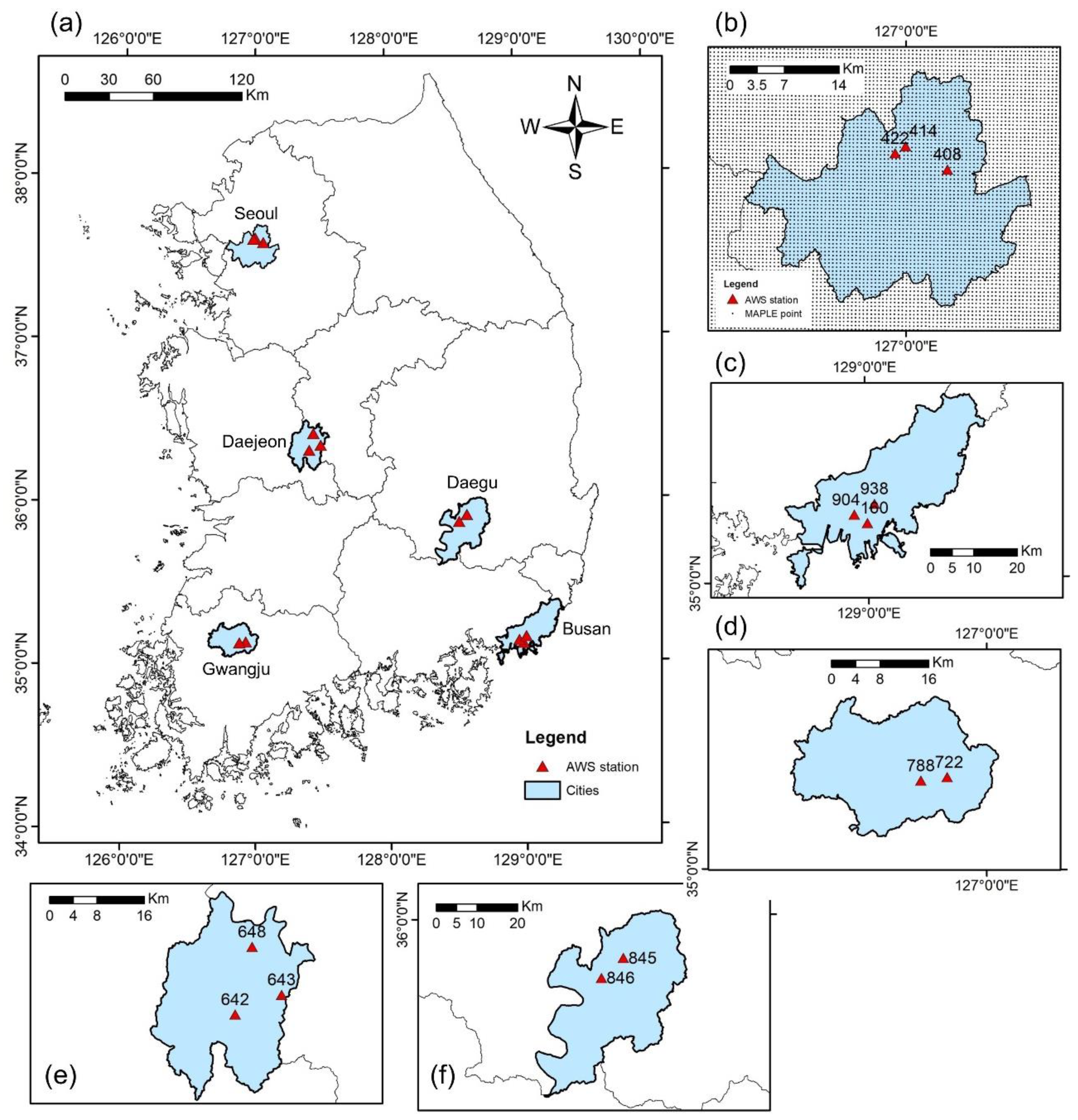
The metropolitan cities in Korea are highly urbanized with a large density of commercial, industrial, and residential areas. Figure 1 presents the location of five urban areas in South Korea, rain gauges, and MAPLE data points. The rain gauges used in this study belong to the Automatic Weather System (AWS) that is controlled by the Korean Meteorological Administration (KMA). In Figure 1, the rain gauges are denoted by red triangles and MAPLE data points are denoted by black dots. In this study, the cities such as Seoul, Busan, Gwangju, Daejeon, and Daegu are selected as the study areas (Figure 1a). In the cities, urban floods occur fast during a few hours in the strong rain events. The events usually appear from June to September. The rain gauges located in the urban areas are chosen to examine the proposed models.

2.2. Data Collection

Measured rainfall from 13 arbitrarily selected gauges of the AWS named 408, 414, and 422 (in Jeonnong, Seoul); 160, 904, and 938 (in Busan city); 722 and 788 (in Gwangju city); 642, 643, and 648 (in Daejeon city); 845 and 846 (in Daegu city) was obtained from the KMA website for training and testing. All AWS stations are recorded with a temporal resolution of 1 min. A selection of heavy rainfall events pertinent to the period from 2016 to 2020 was chosen and analyzed. All the rainfall events have a short duration (less than 12 h). The thresholds regarding maximum 10 min rainfall intensity ($\ge 5\mathrm{mm}/10\min$) and 6 h accumulated rainfall ($\ge 45\mathrm{mm}$) were applied to define a heavy rainfall event [37,38]. Consequently, twenty-seven heavy rainfall events that normally occur from June to September were chosen. Based on these selected events, twenty-two events were chosen for calibration and validation in the training session and five events were used for the test stage.

Table 2. The heavy rainfall events used in this research.

No.	Event	Duration (hour:min)	Maximum Rainfall in AWS Stations (mm/10 min)	City	Configuration
1	20160701	19:00–22:30	8.5	Seoul	Training and Validation
2	20160704	1:00–7:00	16.0	Busan
3	20160705	8:00–11:00	18.5	Seoul
4	20160729	6:00–9:00	13.5	Seoul
5	20170702	21:00–2:00	15.5	Seoul
6	20170710	19:00–23:00	13.5	Seoul
7	20170715	3:00–7:00	12.5	Seoul
8	20170815	9:00–16:00	8.0	Seoul
9	20170820	21:00–24:00	12.5	Seoul
10	20170825	4:00–7:00	15.0	Gwangju
11	20180628	4:00–16:00	8.5	Busan
12	20180810a	2:00–8:00	11.0	Daegu
13	20180810b	18:00–22:00	15.0	Gwangju
14	20180827	9:00–16:00	15.5	Gwangju
15	20180828	15:30–21:30	17.5	Seoul
16	20180829	16:00–7:00	9.0	Seoul
17	20180831	9:00–12:00	19.0	Gwangju
18	20190720	1:00–18:00	8.0	Busan
19	20190726	6:00–13:00	7.5	Seoul
20	20190804	17:00–19:00	14.0	Seoul
21	20200610	22:00–3:00	8.5	Daejeon
22	20200629	16:00–2:00	7.0	Busan
23	20170723	7:00–12:00	13.5	Seoul	Test
24	20180826	17:00–1:00	12.0	Daejeon
25	20180904	0:00–4:00	10.0	Gwangju
26	20190731	6:00–10:30	15.5	Seoul
27	20190806	14:00–21:00	6.5	Busan

Note: The temporal resolution of the rain events is 10 min. The time unit is denoted by “hour:min” in the “Duration” column.

illustrates the selected events used in this work. Simultaneously, forecasted data of the MAPLE system were also collected and processed to provide sequential inputs for the models.

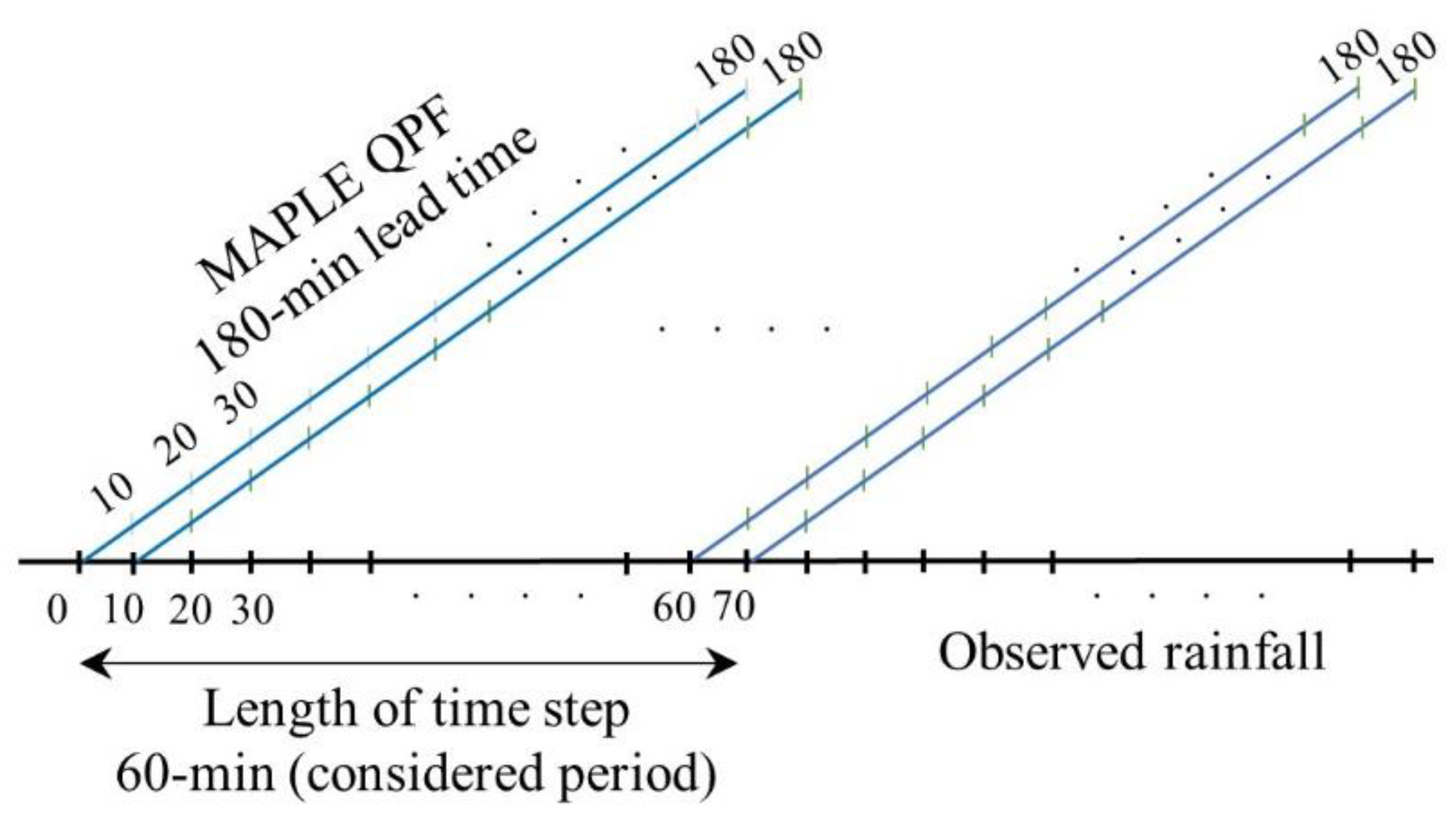
In this research, the radar-based forecast data from the MAPLE system operated by The Han River Flood Control Office (HRFCO) was used. The system applied in the dual-polarization radar network that generates 360 min QPFs every 10 min with a temporal resolution of 10 min. The domain of the system is 1050 × 1050 pixels with a spatial resolution of 0.5 km. Figure 1b displays the data points of the MAPLE system that overlap with Seoul city. In this work, the 180 min QPFs were deployed to develop the data-driven models due to the high uncertainty of the MAPLE data with 360 min forecast time and a short period of the examined rain events. The QPFs of twenty-five data points surrounding each AWS station were utilized as the input of the selected data-driven models. For the training session, the total considered time step of the QPFs of the data points was 60 min from the beginning of each rainfall event. Thus, the considered number of time steps of QPF was six for a selected event. The number of time steps of the MAPLE QPF can be varied depending on the period of each rainfall event and experimental results.

While the radar-based forecast data have a temporal resolution of 10 min, the measured rainfall at the gauges has a temporal resolution of 1 min. Therefore, the measured rainfall was accumulated to obtain 10 min temporal resolution of rainfall after using the inverse distance weight (IDW) method [39] to correct the missing rainfall data. The observed 10 min rainfall data were utilized herein as the output of machine learning methods for the training stage. To ensure the correspondence between the input and output of the models, the forecast rainfall of the data points and observed 10 min rainfall should have the same time order. Figure 2 presents the method of preparing the QPF data as the input and observed rainfall as the correct value for the data-driven models in the training stage. Notably, all the surrounding spatial–temporal data points at each AWS station were considered as an input matrix for the models. The detailed process regarding training datasets and model implementation is presented in Section 3.5.

3. Methodology

3.1. Multivariate Adaptive Regression Splines (MARS)

As a nonlinear and non-parametric approach, MARS was first introduced for predicting a continuous dependent variable [40], and it recognizes nonlinear patterns of interest embedded in the dense datasets. MARS uses a set of basic functions and coefficients that is driven by data regression to construct the relationship between the variables. This process can be achieved by conducting a forward–backward procedure [41].

In the forward stepwise phase, the model added a considerable number of the basic functions that eventually leads to overfitting of the data. The functions of the MARS algorithm rely on a segment (spline) function that divides the set of data into different linear splines. At fixed points (known as knots), spline functions are joined. The MARS model can generally be defined as follows:

$$f\left(x\right)=c_0+{{\displaystyle \sum }}_{n=1}^N{c}_n{B}_n\left(X\left(t\right)\right),$$

(1)

where $X\left(t\right)=\left\{X_{t1}, \dots , X_{tn}\right\}$ denotes the twenty-five predictor variables corresponding to twenty-five spatial grids in a 10 min time step, $c_0$ is the bias, $B_n\left(x\right)$ denotes the nth basis functions, $c_n$ represents the coefficients of the $B_n\left(x\right)$ that use the least square approach for estimating the values, and N denotes the total number of functions and coefficients of the last model generated in the forward–backward procedure. Unnecessary basic functions are removed in the backward step by using the generalized cross-validation method to enhance the quality of the forecast; thus, the final number of functions (N) are defined. The detailed information about the MARS algorithm can be referred to in the articles [21,22,40,41].

3.2. Multi-Layer Perceptron (MLP)

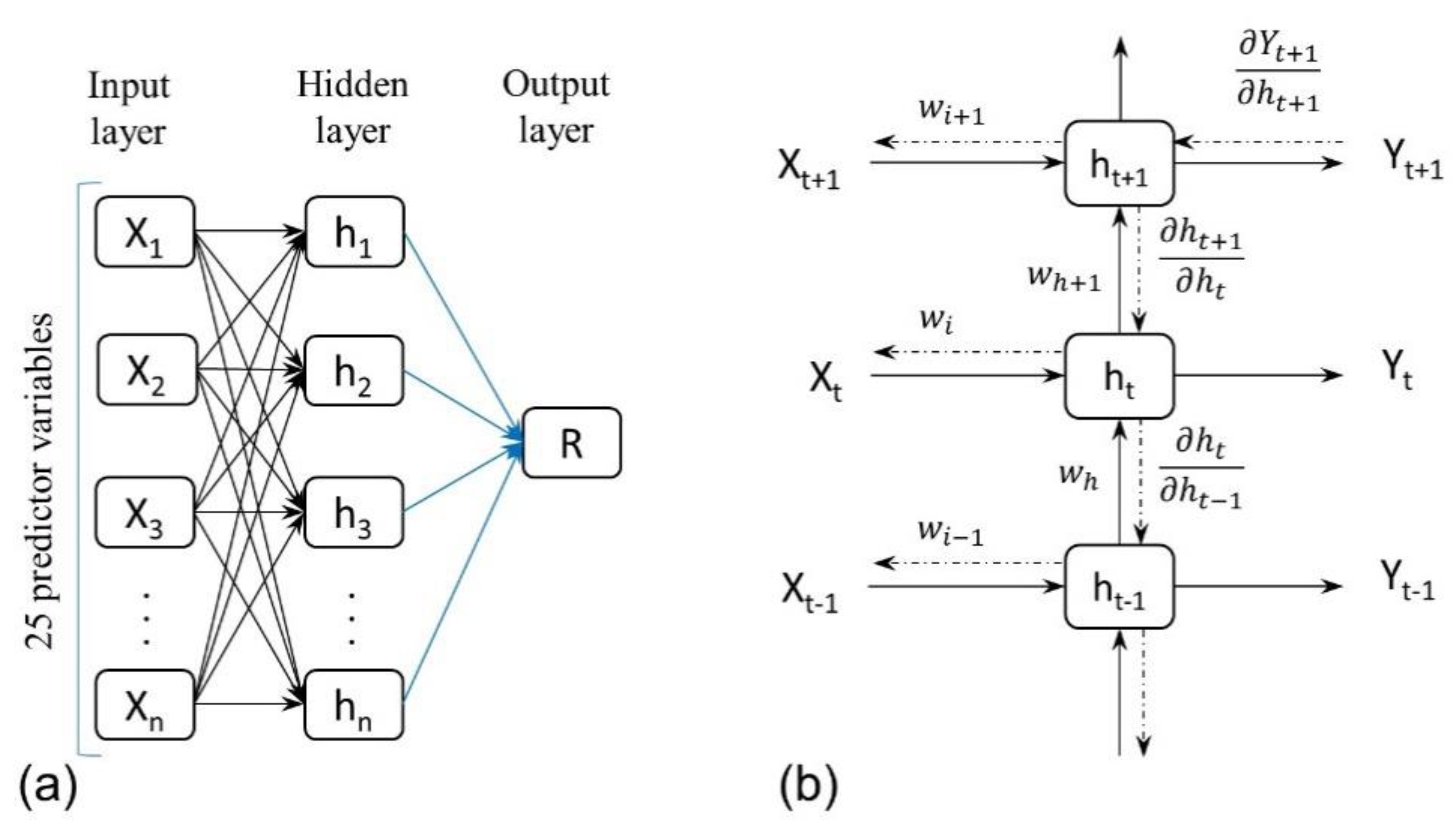
The MLP model is the most popular type of ANNs, and it normally consists of one hidden layer, one input layer, and one output layer [32]. The structure of a classical three-layered MLP is shown in Figure 3a. In the MLP network, the disparate layers are linked by weights and bias, and some neurons are contributing to each layer. In Figure 3a, the rectangles are designated as neurons and the lines between rectangles are designated as weights. Firstly, the MLP calculates the weighted sum of the inputs that is expressed by the following equation.

$$z={{\displaystyle \sum }}_{i=1}^n{w}_i·X_i+b,$$

(2)

where $z$ represents the weighted sum which represents fed into the neuron, $w_i$ represents the weights, $X_i$ represents the input included the twenty-five predictor variables, and b represents the bias. The MLP must be set for nonlinear activation functions. Herein, the common sigmoid for any variable $s$ is adopted as the hidden transfer function and output layer transfer function that is defined as follows:

$$\mathrm{f}\left(s\right)=\frac{1}{1+e^{-s}},$$

(3)

The backpropagation (BP) technique is popularly utilized for training the MLP model. The network is trained to optimize the cost function:

$$F=\frac{1}{2}{\left(f\left(z\right)-f{\left(z\right)}_{observed}\right)}^2,$$

(4)

where $F$ represents the function cost, $f\left(z\right)$ represents the predicted value from a neuron, and $f{\left(z\right)}_{true}$ represents the observed value as the desired output.

The chain rule of differentiation is used in BP for estimating the partial derivative of the error of the corresponded weights. The change rate of the cost F concerning a weight $w_i$ is formulated as follows:

$$\frac{\partial F}{\partial w_i}=\frac{\partial F}{\partial f\left(z\right)}\frac{\partial f\left(z\right)}{\partial z}\frac{\partial z}{w_i},$$

(5)

The partial derivative of the activation function can be represented by the following formulation.

$$\frac{\partial f\left(z\right)}{\partial z}=f\left(z\right)\left(1-f\left(z\right)\right),$$

(6)

The partial derivative of the cost function is represented by Equation (7):

$$\frac{\partial F}{\partial f\left(z\right)}=f\left(z\right)-f{\left(z\right)}_{true},$$

(7)

The training of the MLP network means the weights are iteratively adjusted by using the BP algorithm to calculate errors between the predicted and true value.

3.3. Basic RNN and Long-Term Dependencies Problem

RNNs have a superiority for sequential information in data. RNNs define the present state by the input $X_t$ and the output state of the preceding time step $h_{t-1}$ [30,42]. The state formulations for the time steps t and t + 1 are presented as follows:

$$h_t=\sigma \left(w_h{h}_{t-1}+w_i{X}_t+b\right),$$

(8)

$$h_{t+1}=\sigma \left(w_{h+1}{h}_t+w_{i+1}{X}_{t+1}+b\right),$$

(9)

where $\sigma$ is the activation function, $h_{t-1}$, $h_t$, and $h_{t+1}$ are the states of hidden neurons for the time steps t − 1, t, and t + 1, respectively; $w_{h+1}$ and $w_h$ denote the weights of hidden neurons; $w_{i+1}$ and $w_i$ denote the weights of input layer and hidden layer; $b$ denotes the bias. Notably, each input $X_t=\left\{X_{t1}, \dots , X_{tn}\right\}$ at time step $t$ includes the twenty-five predictor variables at every time step that are the same as the above-mentioned models. From Equations (8) and (9), the difference between RNN and MLP is that the RNN obviously considers the state of previous time step, whilst the MLP has independent output and input at every time step.

For training RNNs, the backpropagation through time (BPTT) method is implemented as an innovative version of BP algorithm in which the chain rule of differentiation is used for calculating the partial derivative of the error of the corresponded weights [32]. Figure 3b shows the scheme of the BPTT algorithm and the structure of the RNN that includes one hidden layer, an input layer, and an output layer. BPTT determines both the partial derivative of the cost concerning the input weights and the partial derivative of the cost with respect to the hidden weights of the previous state. As seen in Figure 3b, the dash-dot line denotes the gradient computation of the BPTT algorithm. Firstly, BPTT calculates the partial derivative of the output at time step t + 1 considering the state of the hidden neuron at time step t + 1 ($\frac{\partial Y_{t+1}}{\partial h_{t+1}}$ in Figure 3b). Afterward, it calculates the partial derivative of the state of hidden neuron at time step t + 1 concerning the state at preceding step ($\frac{\partial h_{t+1}}{\partial h_t}$ in Figure 3b). The partial derivative of the error E considering a weight $w_i$ then sums up the contributions at every time step and can be expressed as follows:

$$\frac{\partial E_{t+1}}{\partial w_i}={{\displaystyle \sum }}_{k=0}^{t+1}\frac{\partial E_{t+1}}{\partial Y_{t+1}}\frac{\partial Y_{t+1}}{\partial h_{t+1}}\frac{\partial h_{t+1}}{\partial h_k}\frac{\partial h_k}{\partial w_i},$$

(10)

where $Y_{t+1}$ is the predicted value from the neuron. The BP process continues to the former neurons step by step in the same manner.

The error of partial derivative increases gradually with the time step when conducting gradient estimation in the BPTT method. Subsequently, the gradient over many time steps of the network can be very small or can be very large [30]. The phenomenon is called the vanishing/exploding gradient problem. Therefore, determining how to learn and tune the hyper-parameters of the hidden layer for capturing long sequential data may be highly complex and could lead to overtraining times.

3.4. LSTM Network

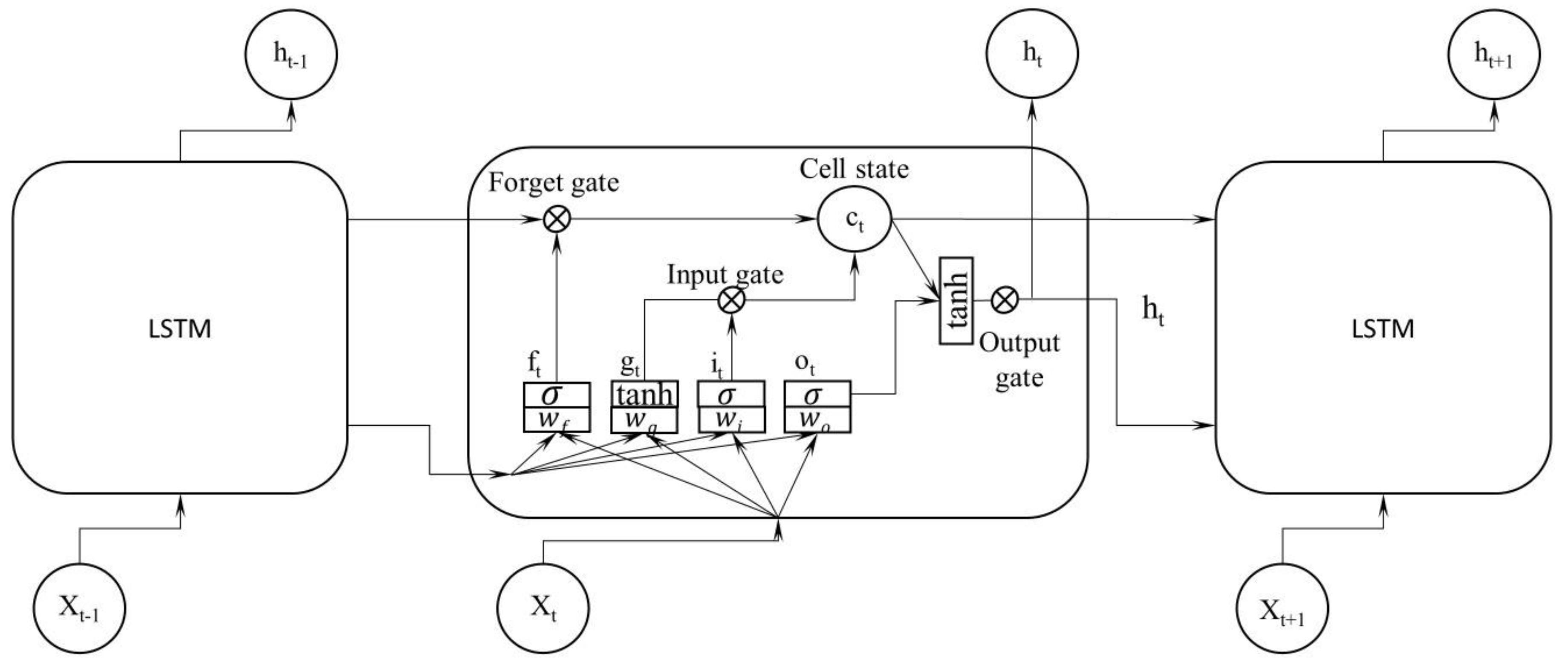
The LSTM-cell can solve the vanishing/exploding problem of the BPTT algorithm when training a long-term sequence [30,43]. Unlike the simple RNN cell, each LSTM cell typically has four layers composed of the main layer called the gate of input modulation (g) and three gate controllers for optionally letting information through by an activation function and a pointwise multiplication operation: input gate (i), forget gate (f), and output gate (o). Therefore, LSTMs are able to carry this information for long-term dependencies. LSTMs can drop some unimportant memory or add some new content, learn the long-term state, and then filter the result. Figure 4 shows the structure of the LSTM unit in the RNN hidden layer. The symbol c denotes the memory cell. The LSTM algorithm can be shown by the below equations:

$$i_t={\sigma }_s\left(w_{hi}{h}_{t-1}+w_i{X}_t+b_i\right),$$

(11)

$$f_t={\sigma }_s\left(w_{hf}{h}_{t-1}+w_f{X}_t+b_f\right),$$

(12)

$$o_t={\sigma }_s\left(w_{ho}{h}_{t-1}+w_o{X}_t+b_o\right),$$

(13)

$$g_t=tanh\left(w_{hg}{h}_{t-1}+w_g{X}_t+b_g\right),$$

(14)

Cell state:

$$c_t=f_t°c_{t-1}+i_t°g_t,$$

(15)

Output vector:

$$h_t= y_t= o_t°tanh\left(c_t\right),$$

(16)

where $X_t=\left\{X_{t1}, \dots , X_{tn}\right\}$ represents the input vector that includes twenty-five variables represented the corresponded to data points surrounding the stations at time step $t$; $b$ and $w$ denote parameters for bias and weights, respectively; $°$ is the element wise multiplication of two vectors; $tanh\left(z\right)=\frac{e^z-e^{-z}}{e^z+e^{-z}}$ is the hyperbolic tangent function; ${\sigma }_s\left(z\right)=\frac{1}{1+e^{-z}}$ is the sigmoid function.

In Equations (11)–(16), $h_t$ can be considered as the short-term state and $c_t$ can be considered the long-term state. In brief, LSTMs can control exploding information largely because sigmoid activation is used as the gating function for 3 gates, which present outputs between 0 and 1, which does not allow for the flow of information (with a value of 0) or allows for the complete flow of information (with a value of 1). To avoid the dissipating gradient issue, the $tanh$ function is used to for maintaining the second derivative over a prolonged extent before approaching zero. Therefore, with these types of systems, a value very far from the past may be valid in the LSTM predictions. Mathematically, the LSTM recurrent networks first use the previous hidden state for gaining the fixed-dimensional proxy of the sequential input to estimate the conditional probability, and then define the probability of its corresponding output sequence with the initial state, which is set to the representation of the input sequence [44]. These properties ensured that the LSTM was the dominant model.

3.5. Training Datasets and Model Implementation

For the 27 selected events (Table 2), 22 events were chosen for training and validating sets and the other 5 events were used for testing sets. The training sets were arranged from the 1st event to 22nd event as continuous time series data. The considered period of the MAPLE QPFs was approximately 60 min at the beginning of each event (as shown in Figure 2). The considered period of an event can be changed to smaller than 60 min because of the short period of the strong rainfall events. In this study, we separately developed forecast time models corresponding to 60 min, 120 min, and 180 min lead time. Therefore, the QPF data used in the 60 min, 120 min, and 180 min models had a 60 min lead time, 120 min lead time, and 180 min lead time, respectively. The input matrices of the different forecast time models include 25 columns for the number of QPF data points that are overlaid with each AWS station. Simultaneously, the vector output includes one column representing the observed rainfall at the corresponding ground stations and was provided in the same time order as the input (Equation (17)). The vector output was also issued separately according to the different forecast time models. Notably, the data used in five algorithms (MLR, MARS, MLP, basic RNN, and LSTM) are similar in terms of data structure and temporal scale. The input and output for each lead-time model can be explained as follows:

$$\left\{\begin{array}{c}{X}_{1,10,1}^1, \dots , X_{1,10,n}^1\\ ⋮\\ X_{1,lt,1}^1, \dots , X_{1,lt,n}^1\\ ⋮\\ X_{qe,lt,1}^e, \dots , X_{qe,lt,n}^e\end{array}\right\}~\left\{\begin{array}{c}{Y}_{1,10}^1\\ ⋮\\ Y_{1,lt}^1\\ ⋮\\ Y_{qe,lt}^e\end{array}\right\}$$

(17)

where $X$ is forecasted rainfall of the MAPLE; $Y$ is observed rainfall at the corresponding gauge; $e$ is the $e$-th event; $qe$ is the number of selected QPFs in an event; $lt$ is the selected lead times (60 min, 120 min, and 180 min), for example, with 60 min lead time there are 6 rainfall values corresponded to six 10 min time steps; $n$ is number of variables, in this study, $n=25$ variables that corresponded to 25 data points surrounding a rain gauge at each time step of each QPF.

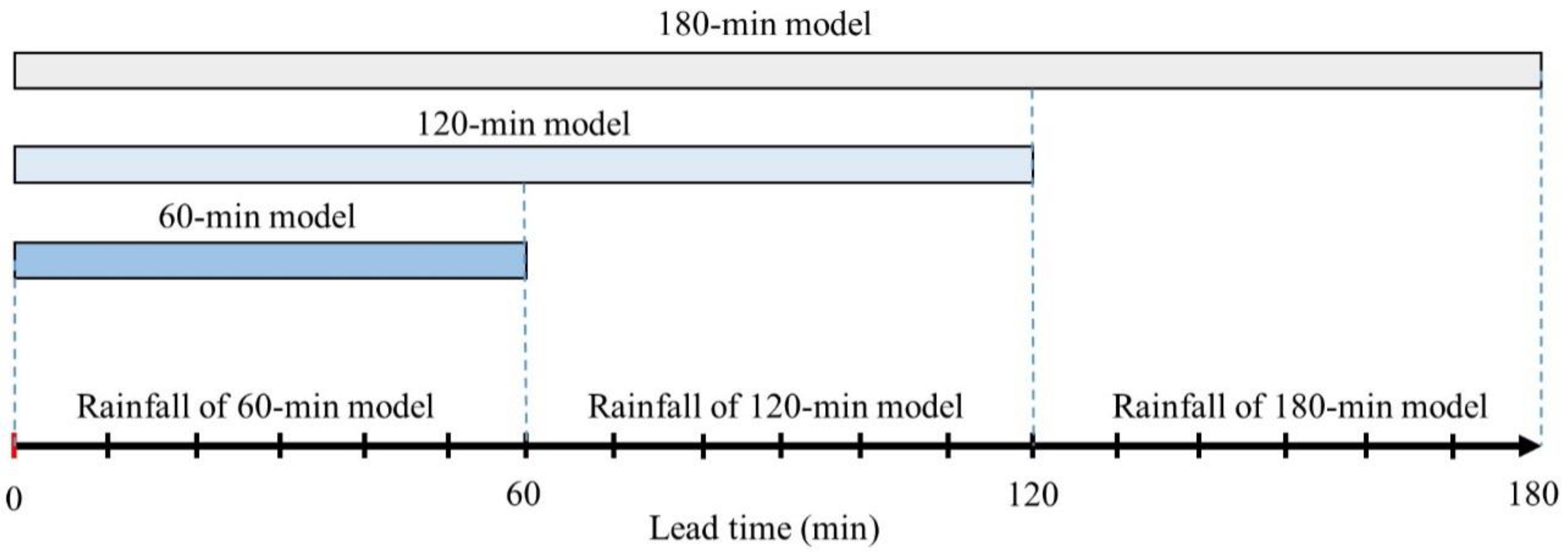
For testing stage, the two time steps of QPF issued from the beginning of each test event were chosen to examine the performance of the AI models and regression-based models because of the short period and zero forecasts in the last time steps of the events. Like the process of training data preparation, these two time steps of QPF were prepared for testing the 60 min, 120 min, and 180 min models. Notably, the time period was fixed at the beginning of the events when implementing the forecast time models to each time step of QPF. In other words, the 120 min model was extended by an additional 60 min compared to the 60 min model, and so on for the 180 min model. The 180 min corrected rainfall results were combined from the test results of three different forecast time models. Figure 5 shows how to combine three models to obtain final 180 min corrected rainfall forecasts. The rainfall of the first 60 min lead time, the rainfall after 60 min to 120 min lead time, and the rainfall after 120 min to 180 min were based on the 60 min model, the 120 min model, and the 180 min model, respectively. The method of combining different lead-time models was applied to all the proposed models in this study.

In this study, the ANN models were developed based on version 2.3.0 of open-source Tensor-Flow [45] that is a machine learning program published by Google. Besides, the other packages of Python programs, namely Numpy [46], sklearn [47] and Matplotlib [48], were applied. The hyper-parameters were used to calibrate the model, for example, the neural number of each hidden layer and batch size. The number of iterations can be determined from the training loss and validation loss performance.

3.6. Model Performance Parameters

The performance of the proposed models is evaluated by indicators, including the critical success index (CSI), probability of detection (POD), percent error in maximum rainfall (PEMR), root mean square error (RMSE), correlation coefficient (R) and relative forecast bias (FB) as shown in the following equations.

CSI and POD are used as quantitative evaluation parameters to represent the success of forecasts for hit rates. Below equations interpret the calculation of CSI and POD. If the CSI or POD is equal to 1, then the quality of the forecast is excellent.

$$CSI=\frac{A}{A+B+C},$$

(18)

$$POD=\frac{A}{A+B},$$

(19)

where A, B, and C denote the hit, miss, and false alarm number for a examined threshold, respectively.

The RMSE is calculated as follows:

$$RMSE=\sqrt{\frac{{{\displaystyle \sum }}_{i=1}^n{\left(Y_i^{for}-Y_i^{obs}\right)}^2}{n}},$$

(20)

where $Y_i^{for}$ is the i-th forecasted data; $Y_i^{obs}$ is the i-th observed data; n is the number of data. RMSE values equal zero indicate the best fit between forecasted and observed data.

The R value is calculated as follows:

$$R=\frac{{{\displaystyle \sum }}_{i=1}^n\left(Y_i^{for}-Y_{for}^{mean}\right)\left(Y_i^{obs}-Y_{obs}^{mean}\right)}{\sqrt{{{\displaystyle \sum }}_{i=1}^n{\left(Y_i^{for}-Y_{for}^{mean}\right)}^2{{\displaystyle \sum }}_{i=1}^n{\left(Y_i^{obs}-Y_{obs}^{mean}\right)}^2}},$$

(21)

The FB is utilized for assessing the quality of the total forecasted rainfall as follows:

$$FB=\frac{{{\displaystyle \sum }}_{i=1}^n{Y}_i^{for}}{{{\displaystyle \sum }}_{i=1}^n{Y}_i^{obs} },$$

(22)

If the FB is around 1, then the forecast is considered highly accurate. FB values from 0 to 1 indicate an underestimation in prediction, and values larger than 1 show an overestimation.

PEMR is used to examine the capability of the models in maximum rainfall prediction (Equation (23)). In the equation, $Y_{for}^{max}$ and $Y_{obs}^{max}$ are the maximum rainfall values of the forecasted data and observed data, respectively.

$$PEMR=\frac{Y_{for}^{max}-Y_{obs}^{max}}{Y_{obs}^{max}}\times 100,$$

(23)

4. Results and Discussions

4.1. Training of ANN Models

Because the main objective of this study is to improve rainfall forecasts from radar-based forecasting systems for urban areas under heavy rainfall events, different forecast time models of the data-driven methods were developed. The goals of the models are to reproduce rainfall forecasts with a 180 min lead time based on observed rainfall and 25 data points around rain gauges from the MAPLE system. After arranging the input and output data, the trial-and-error approach was applied for tuning the hyper-parameters, such as the neural number of each hidden layer, learning rate, batch size and the iteration number. The dataset was divided into 80% for training and 20% for validation.

A regularization method is essential for the proper performance of the ANN models to prevent overfitting. In this work, early stopping was utilized as a regularization method that is utilized to stop the training process when the validation error reaches a minimum. The optimization algorithm used in the models was the ADAM technique [49]. The learning rate used for the models was 0.005. The RMSE was chosen for measuring the error of model prediction in the training stage. The optimum structure of the LSTM model and basic RNN model had one hidden layer with 10, 16, and 25 hidden neurons corresponding to the 60 min, 120 min, and 180 min RNN models, respectively. The best structure of the MLP was one hidden layer with 10, 15, and 20 hidden neurons for the 60 min, 120 min, and 180 min MLP models. The number of basic functions in MARS was 71, 20, and 5 for the 60 min, 120 min, and 180 min MARS models.

4.2. Performance of Data-Driven Models

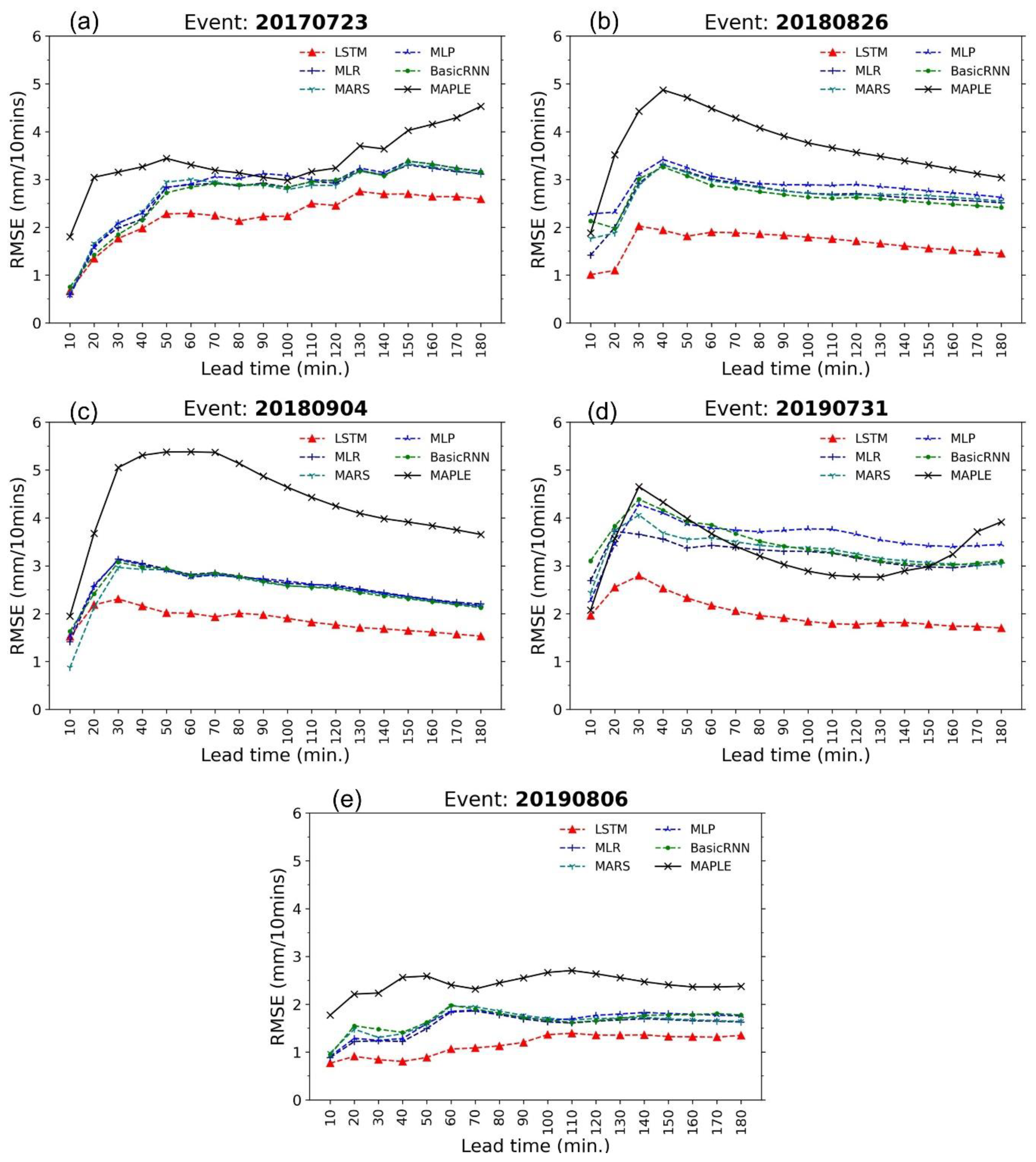
Figure 6 illustrates the RMSE performance of the MAPLE system and the models in the 180 min forecast time. All of the data-driven models showed an improvement with lower RMSE values than the MAPLE, while RMSE values of MAPLE were relatively large in the test events. However, the LSTM model showed the best performances compared with the remaining models. The LSTM model performed a substantial decrease in RMSE in the 180 min lead time of the test events. The maximum decrease in RMSE values of the LSTM for the events was 64.05% compared to MAPLE in the 20180904 event (Figure 6c). The performances of the models MLR, MARS, MLP, and basic RNN showed a notable improvement in comparison with MAPLE for the 4 events 20170723, 20180826, 20180904, and 20190806. In the 20190731 event, the RMSE values of MLP were higher than other correcting models after a lead time of 70 min (Figure 6d). The RMSE values of the models increased notably in the first hour of forecast time in the test events. In the events, 20170723 and 20190806 (Figure 6a,e), the RMSE values of the correcting models increased in 180 min lead time. However, in the three remaining events, after increasing in the first 60 min lead time the RMSE values of the models decreased slowly for the rest of the forecast time (Figure 6b–d). In the two events 20170723 and 20190806, the RMSE of MAPLE showed an upward trend, while in the three remaining events the MAPLE presented a downward trend after 60 min lead time. Those RMSE behaviors of MAPLE are the same as the behaviors of the correcting models. The phenomenon can be explained by the effect of MAPLE input data on the models.

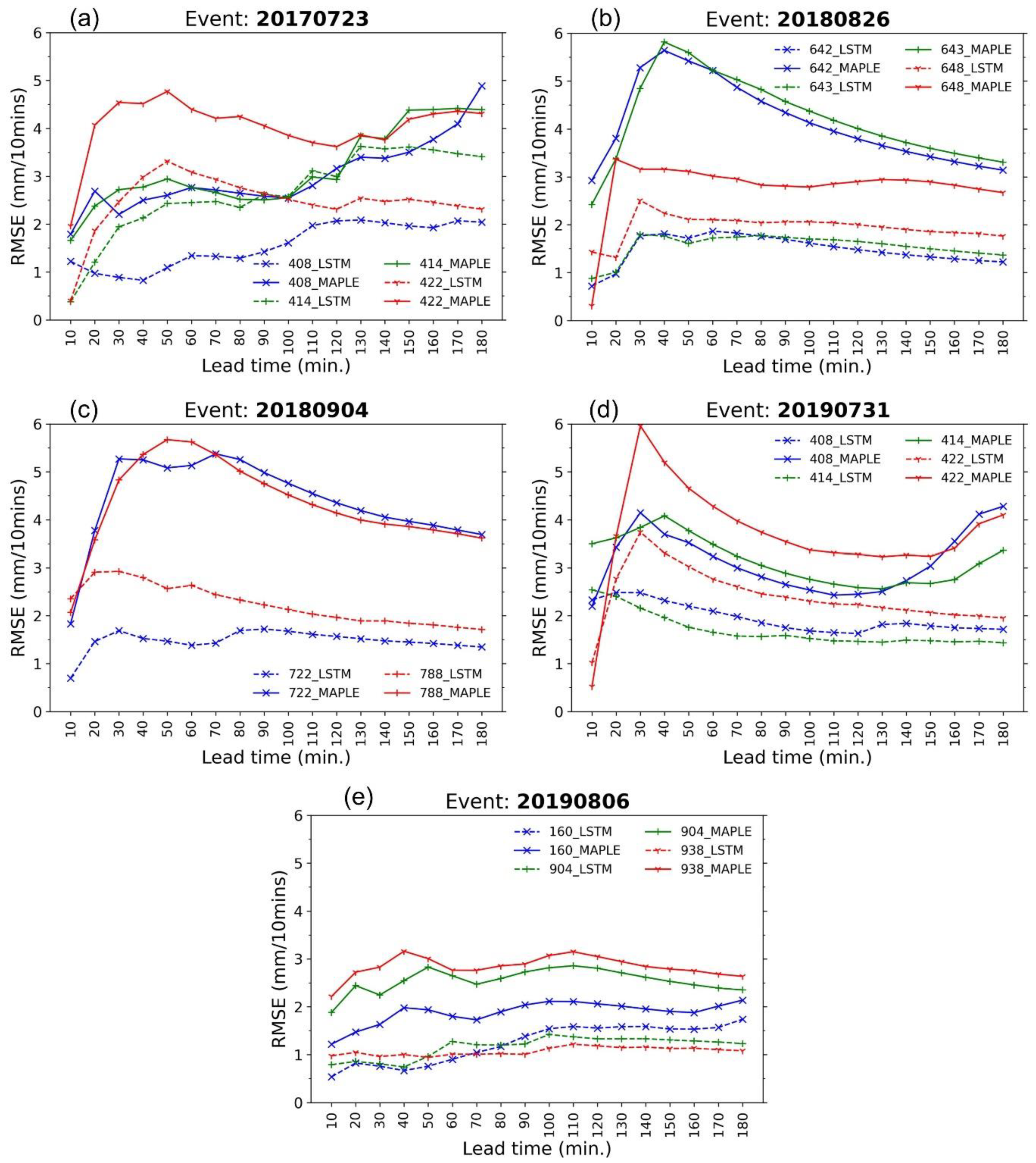
Figure 7 shows the comparisons between MAPLE and the LSTM model in terms of RMSE at the stations. The RMSE values of LSTM at the examined stations were reduced notably compared to the values of MAPLE, especially reducing around 2~3 times at the stations 642 and 643 (in 20180826 event), and 722 (in 20180904 event). The RMSE values of both models increased quickly in 60 min lead time. At most of the stations, the RMSE values of the LSTM model were smaller than that of MAPLE even though they increased rapidly in the 60 min lead time. However, some stations namely 788 (in the 20180904 event), 408, and 422 (in the 20190731 event) had slightly higher RMSE value of LSTM-corrected rainfall than MAPLE at 10 min forecast time.

Table 3. Correlation coefficient of MAPLE and LSTM model within 120 min lead time at the stations in the five test events. The values of each station were estimated by averaging the values of QPFs in each event.

Event	Station	Model	10 min	20 min	30 min	60 min	90 min	120 min
20170723	408	LSTM	0.811	0.92	0.89	0.93	0.60	0.51
		MAPLE	0.01	0.41	0.31	0.47	−0.05	−0.06
	414	LSTM	0.996	0.81	0.47	0.45	0.24	0.29
		MAPLE	0.68	0.22	0.08	0.34	0.47	0.08
	422	LSTM	0.994	0.81	0.80	0.86	0.87	0.82
		MAPLE	0.52	−0.12	−0.15	0.57	0.48	0.27
20180826	642	LSTM	0.98	0.97	0.97	0.95	0.92	0.94
		MAPLE	0.83	0.60	0.59	0.58	0.30	0.48
	643	LSTM	0.99	0.99	0.98	0.95	0.92	0.90
		MAPLE	0.85	0.62	0.48	0.65	0.51	0.47
	648	LSTM	0.35	0.65	0.93	0.62	0.61	0.65
		MAPLE	0.99	0.89	0.83	0.43	0.24	0.11
20180904	722	LSTM	0.98	0.91	0.97	0.96	0.87	0.87
		MAPLE	0.50	0.33	0.62	0.42	0.12	0.25
	788	LSTM	0.53	0.32	0.69	0.74	0.78	0.83
		MAPLE	0.07	−0.18	0.29	−0.03	−0.12	0.20
20190731	408	LSTM	0.93	0.90	0.78	0.80	0.80	0.80
		MAPLE	0.94	0.63	0.18	0.29	0.38	0.39
	414	LSTM	0.04	0.73	0.87	0.90	0.91	0.91
		MAPLE	0.03	0.28	0.31	0.39	0.46	0.47
	422	LSTM	0.98	0.99	0.95	0.92	0.92	0.91
		MAPLE	0.998	0.81	0.68	0.69	0.73	0.70
20190806	160	LSTM	0.01	0.90	0.82	0.92	0.58	0.60
		MAPLE	0.78	0.73	0.48	0.67	0.59	0.59
	904	LSTM	0.98	0.87	0.84	0.77	0.71	0.67
		MAPLE	0.48	−0.04	−0.04	0.18	0.13	0.11
	938	LSTM	0.99	0.85	0.88	0.91	0.83	0.74
		MAPLE	0.75	0.37	−0.18	0.32	0.25	0.20

Note: The computation of the correlation coefficient is started from time step t₋₁₀ in the lead time.

summarizes the comparative results for R values of MAPLE and the LSTM model at the stations in terms of the first 120 min forecast times. The R values were calculated by comparing MAPLE or LSTM to the observations. In general, the performances of the LSTM model at the stations in terms of correlation coefficient were much better than the MAPLE forecast. The correlation coefficients of the LSTM forecasts were much better than those of MAPLE forecasts within the first 60 min lead time. However, at stations 648, 414 (20190731 event), and 160, the R values of LSTM were not better than those of MAPLE in 20 min lead time. It can be seen from the Table 3 that the MAPLE system generated the rainfall forecasts with low, even negative, correlation values after 20 min lead time at the stations 422, 788, 904, and 938. These are caused by the high uncertainty of the MAPLE in terms of modeling the growth, deterioration, and movement of the rain field and when issuing the forecasts in the heavy rainfall events. Therefore, some rainfall forecasts can be uncorrelated and non-linear with varied observations during the lead time.

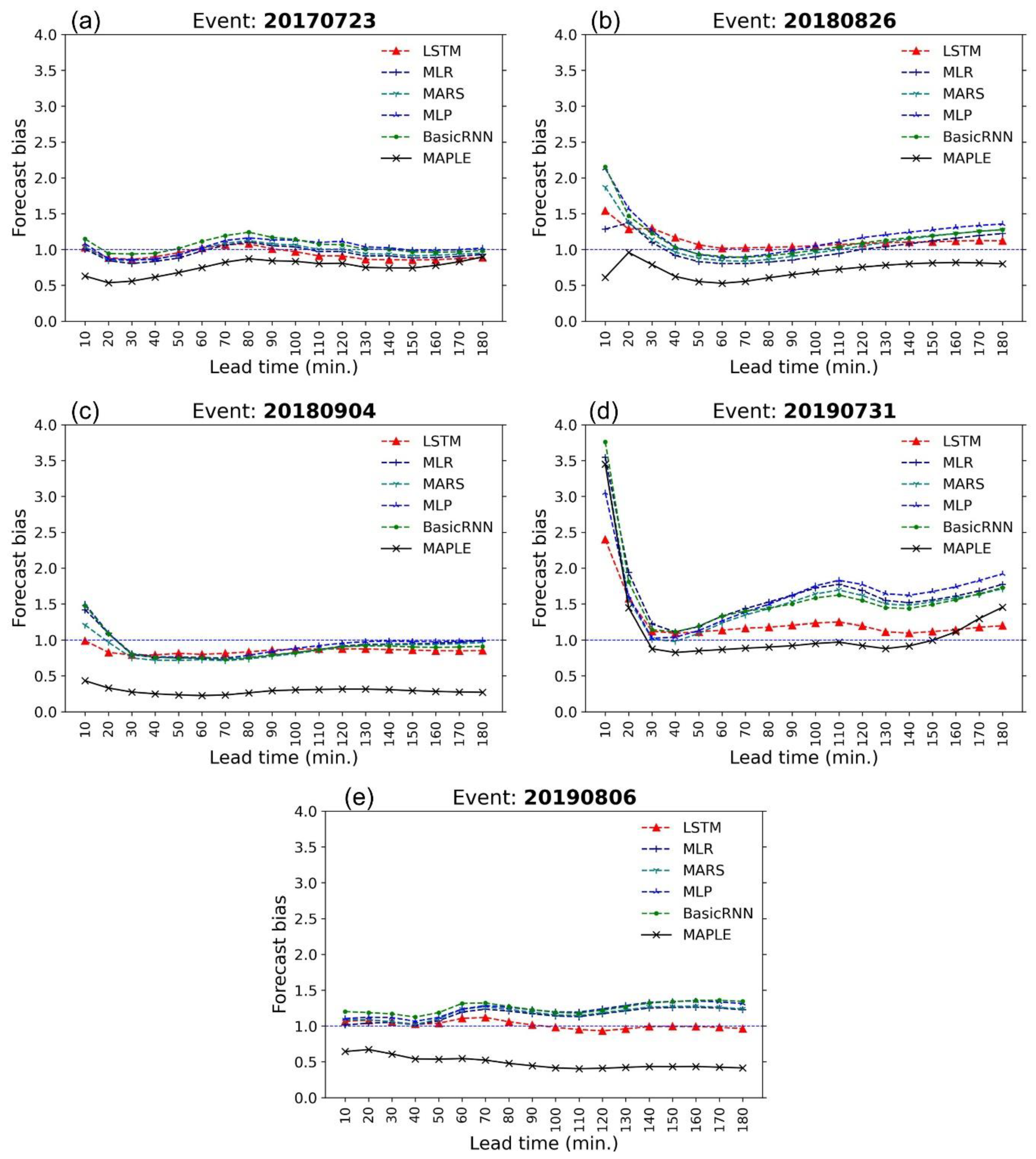
Figure 8 shows the comparative performances of the data-driven models and MAPLE for 180 min rainfall forecasts in terms of FB in 180 min forecast time in the test events. As can be seen, the MAPLE FB is notably and consistently below 1 in four out of the five events, including the events, 20170723 (Figure 8a), 20180826 (Figure 8b), 20190904 (Figure 8c), and 20190806 (Figure 8e). The results of the models showed substantial improvements with FB values closer to the no bias region compared to MAPLE in the 3 test events, 20170723, 20180904, and 20190806 (Figure 8a,c,e). The LSTM showed a slightly better performance than the other models for the events 20170723 (Figure 8a), 20180826 (Figure 8b), and 20180904 (Figure 8c). The LSTM outperformed other models for 20190731 event (Figure 8d) and 20190806 event (Figure 8e) in 180 min forecast time, but only had a slightly better performance than other models at the first 60 min forecast time. Notably, in the event 20190731 (Figure 8d), all the models showed substantial overestimations at the first 30 min and after the 60 min forecast time, however, the performance of the LSTM model was better than that of the correcting models with smaller overestimation. This problem was similar to the first 30 min lead time of the 20180826 event (Figure 8b). In general, the performance of the LSTM regarding FB was more stable and better relative to the other models.

Table 4. Percent error in maximum rainfall (PEMR) of the models in the five test events.

Event	Station	PEMR (%)
		MLR	MARS	MLP	RNN	LSTM	MAPLE
20170723	408	−33.5	−28.1	−13.9	−26.8	1.3	140.7
	414	−50.5	−57.2	−45.0	−54.5	−40.5	−43.7
	422	−54.7	−55.5	−42.8	−52.4	−39.4	−36.3
20180826	642	−50.8	−50.2	−46.2	−46.4	−18.5	−51.9
	643	−51.6	−54.1	−56.8	−51.6	−10.2	−60.8
	648	−12.1	−23.2	−27.6	−10.2	16.0	42.0
20180904	722	−47.3	−45.9	−48.8	−46.1	−26.0	−75.8
	788	−44.9	−40.2	−47.0	−39.4	−23.1	−61.2
20190731	408	−34.9	−18.4	−34.8	−24.4	−16.7	77.1
	414	−28.8	−35.0	3.8	−32.4	−17.5	2.9
	422	−23.1	−46.1	−47.2	−59.9	−40.4	−15.9
20190806	160	−7.0	−3.1	−8.5	6.8	8.2	−24.7
	904	−21.4	−17.8	−22.5	−11.2	16.3	−34.6
	938	−24.5	−17.8	−22.5	−8.5	−9.3	−37.0

summarizes the comparative results for the percent error in maximum rainfall over the stations in the five test events. The LSTM outperformed other models in terms of PEMR at most stations in the test events. While the other correcting models mainly provided the large underestimations of PEMR in the events, the LSTM reproduced the good predictions with a range of −26.0~16.3% of PEMR at most stations. This PEMR improvement of LSTM is considerable for applications of predicting heavy rainfall events and urban flood warning practices. However, some stations had a considerable underestimation of maximum rainfall, namely 414 (−40.5% in the 20170723 event), and 422 (−39.4% and 40.4% in the 20170723 event and 20190731 event, respectively). The basic RNN and MLP models generated good PEMR values at some stations in the events, such as 3.8% (station 414 in 20190731 event) and −8.5% (station 160 in 20190806 event) for MLP, 6.8% and −8.5% (station 160 in 20190806 event) for basic RNN. The original MAPLE forecasts showed significant underestimation in many stations and high overestimation in some stations. This drawback of MAPLE is caused by the rapid growth or decay of rain cells in heavy rain events. Hence, the MAPLE may issue the predictions with much higher or much lower rainfall than the actual rainfall level.

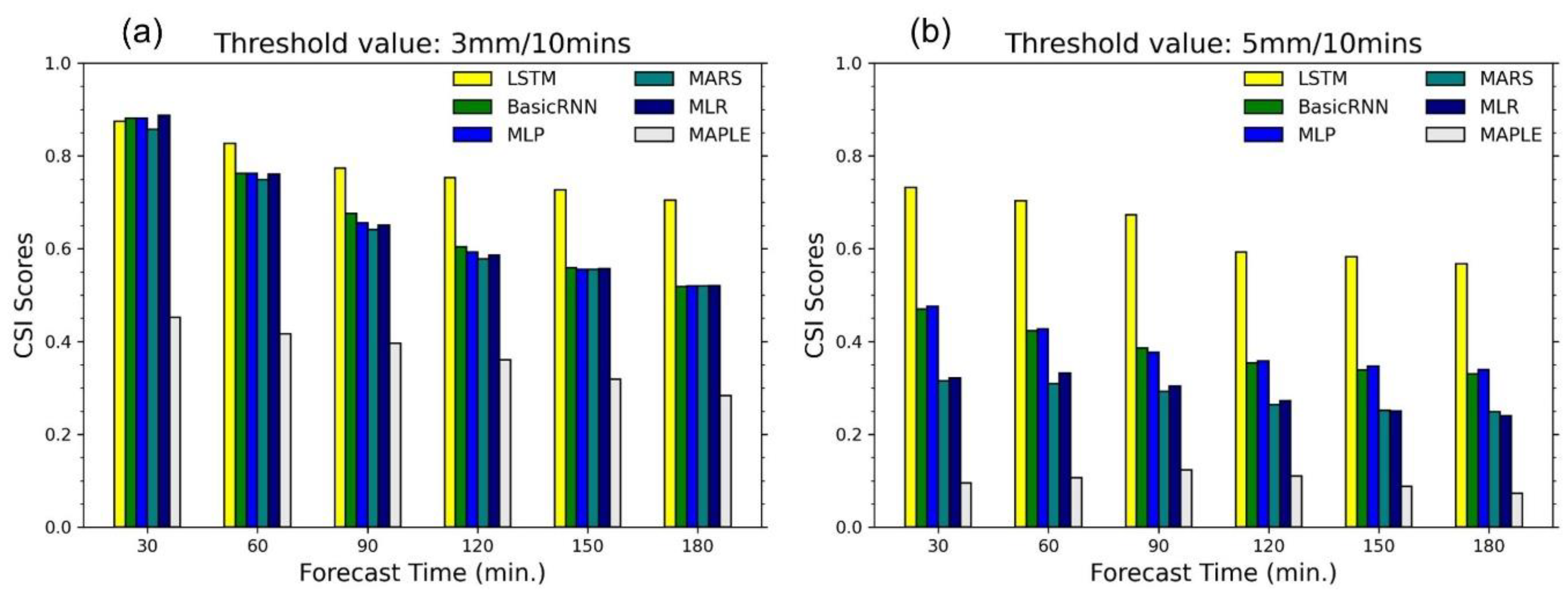
To further investigate the performance of the models, the CSI and POD parameters were estimated by two high thresholds: 3 mm/10 min, and 5 mm/10 min. Figure 9 shows comparisons between MAPLE and the models regarding the CSI with the two thresholds. These comparisons were conducted based on an aggregation of the five test events and eleven test stations over the 180 min forecast time. In detail, the CSI values were estimated from hit, miss, and false alarm along 180 min lead time of predictions at a rain gauge. Then, taking the average values of all rain gauges and events during the 180 min lead time. Concerning the threshold of 3 mm/10 min (Figure 9a), while the CSI values of MAPLE varied from 0.45 to 0.28 in the 180 min lead time, the LSTM, basic RNN, MLP, and MARS showed notable enhancements. However, the LSTM outperformed the other models, with CSI values ranging from 0.88 to 0.71, which are around 2.0~2.5 times higher than the MAPLE’s values along the lead time. The other correcting models had similar performances with their values varying from around 0.89 to 0.53 in the 180 min lead time. For the threshold at 5 mm/10 min (Figure 9b), the CSI values of the LSTM were considerably decreased to the range (0.74, 0.58), while the values of the other models were around 2 times lower than those of the LSTM. Noticeably, the CSI values of basic RNN and MLP ranging from 0.48 to 0.34 were slightly higher than those of MARS and MLR in range (0.32, 0.25). The CSI values of MAPLE were very low, which varied around 0.1.

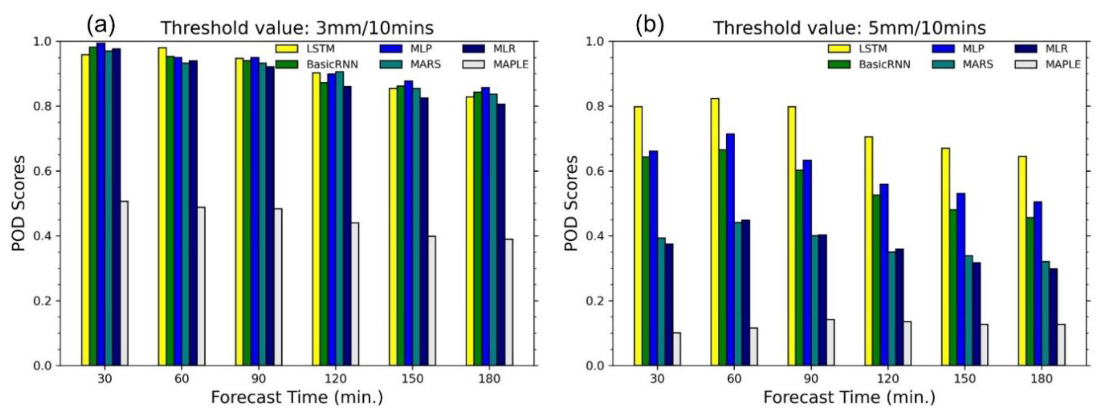
Figure 10 presents the comparative results between MAPLE and the other models in terms of the POD with the two thresholds. For the two thresholds, the performances of the models in terms of the POD were consistent with that of the CSI, with the LSTM outperforming the other models and showing a substantial increase in the POD values at the 5 mm/10 min threshold. However, the POD values of the LSTM and other correcting models at the 3 mm/10 min threshold were similar to each other. Notably, Figure 9 and Figure 10 show that the ANN models are better than the regression-based models in terms of the CSI and POD indicators at the higher threshold. From Figure 9 and Figure 10, the CSI and POD values of MAPLE and the correcting models decreased with the lead time and were substantially reduced when considering at the higher threshold (5 mm/10 min) compared to the lower threshold (3 mm/10 min). While the original MAPLE, MLR, MARS, MLP, and basic RNN performed a rapid decrease from the 3 mm/10 min to 5 mm/10 min thresholds, the LSTM provided a moderate reduction in terms of CSI and POD in the 180 min lead time.

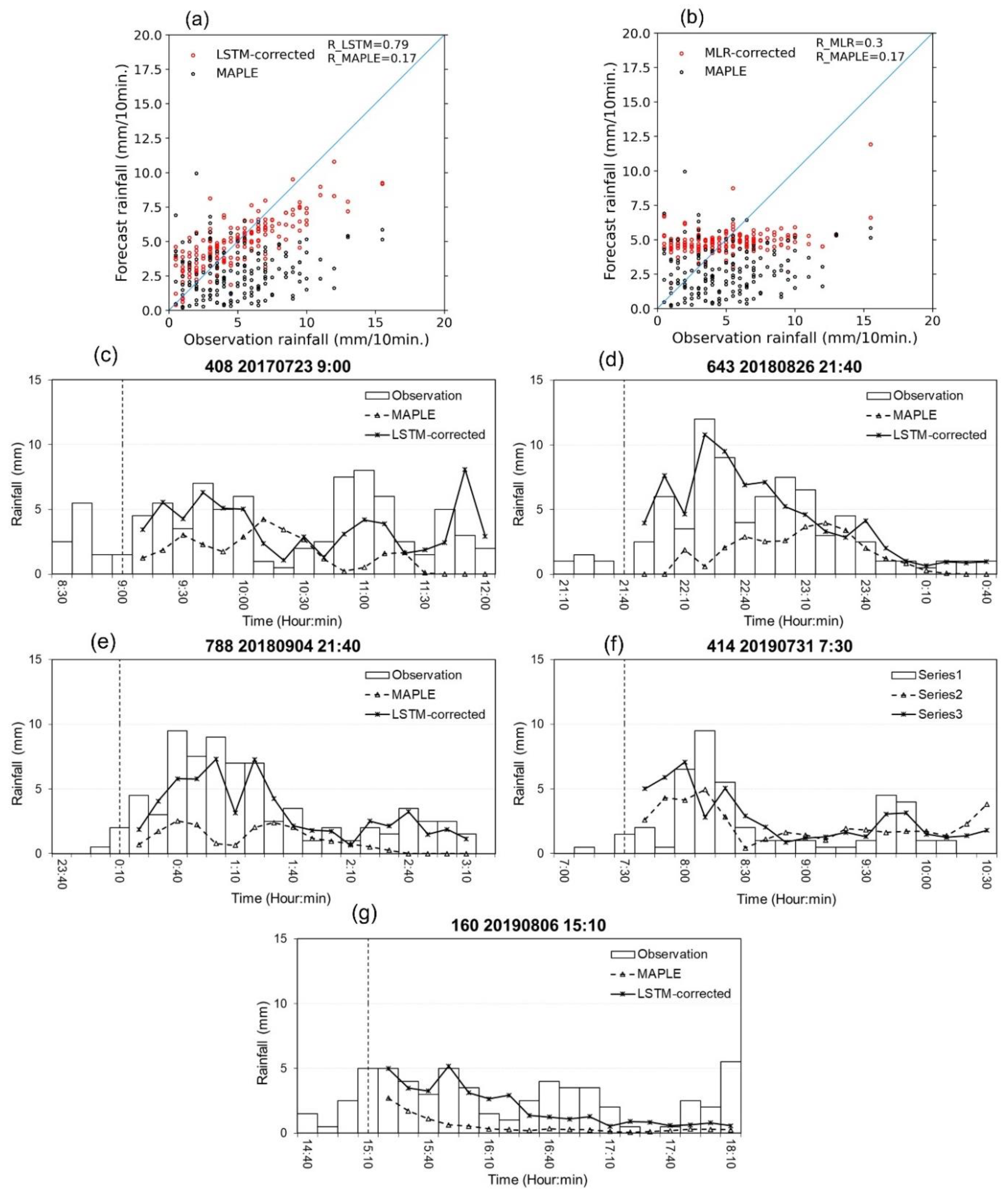
Figure 11 shows the scatter plots of LSTM and MLR with MAPLE in the first 60 min lead time and rainfall patterns of MAPLE and LSTM-corrected rainfall forecast in the test events. As can be seen, while the MAPLE showed a bad correlation with the observations, the LSTM-corrected rainfall forecast showed a fairly good correlation with the observations (Figure 11a). The relationship between LSTM and the observations is moderately strong and positive. Most points of LSTM are fairly close to the best-fit line even at high rainfall values. The MLR did not improve significantly in correlation with the observations. The points of MLR at small rainfall and high rainfall were quite far from the best-fit line (Figure 11b). Figure 11c–g represent rainfall time series from MAPLE, LSTM, and observations at some stations. From these figures, the LSTM-corrected rainfall forecasts for the stations in the test events generally performed better than MAPLE, especially in the first 1.5 h of the forecast time. The MAPLE rainfall time series often showed a large underestimation at high rainfall observations. The LSTM rainfall time series was similar to the rainfall pattern of the observations, especially at times of high rain in the 20180826 event (Figure 11d) and 20180904 event (Figure 11e).

The above results prove that the accuracy of the LSTM-corrected rainfall forecasts is more stable and better than that of the basic RNN, MLP, MARS, and MLR for the 180 min lead time. Thanks to the innovations of the memory cell for managing short-term states and long-term states, the LSTM could provide acceptable performance in terms of correcting rainfall forecasts. The performance was presented by lower RMSE values, better correlation coefficients at high thresholds, higher CSI and POD values, and more reasonable PEMR and rainfall patterns than other models in the test events. In addition, this model takes advantage of training long sequence data; hence, this could lead to good predictions. Notably, the model performances were dependent on the MAPLE forecast data. Specifically, the slight overestimation phenomenon in the events, 20180826 (Figure 8b) and 20190731 (Figure 8d) occurred when MAPLE rainfall forecasts were near no bias zone or overestimation. Additionally, the behavior of RMSE values of the models was quite similar to the RMSE trends of MAPLE (Figure 6). The quick increases in RMSE in 60 min lead time and decreases in CSI and POD values at a threshold of 5 mm/10 min from MAPLE and the correcting models can be explained by the limitations of the MAPLE system. The radar-based extrapolation algorithms do not consider the life cycle of rain cells, especially in convective rain fields. Therefore, the algorithm often fails to forecast rain fields after 60 min or after a few tens of minutes of lead time.

As a result of the uncertainties regarding radar-based systems, the LSTM does not always perform better than the other models, such as degraded RMSE values at stations 414 and 422 in the 20170723 event (Figure 7a), and degraded R values at stations 648, 414 (20180904 event), and 160 (Table 3). Additionally, for the 20190731 event at stations 414 and 422, the PEMR values of LSTM indicated lower maximum rainfall predictions than other models (Table 4). Based on the POD results, although the values were slightly higher compared with the other models when considering the threshold of 5 mm/10 min (Figure 10b), the performance of the LSTM model was not superior to the other correcting models at the smaller threshold (Figure 10a). Moreover, there were several stations, such as 414 (in the 20170723 event) and 422 (in the events: 20170723 and 20190731) that had notable underestimations in forecasting maximum rainfall (Table 4). In this study, the models were trained with data of twenty-five data points surrounding rain gauges; therefore, this is a limitation for generating the rain field. However, it might be overcome by utilizing convolutional neural networks with the full images of overall domain and radar data.

5. Conclusions

To improve hydrological predictions for urban catchments, it is essential to correct the short-term radar-based rainfall forecasts in advance. Such corrections could enable better forecasts and higher efficiencies in urban hydrology. Through examining AWS rain stations of urban areas in Korea, the current work compared the performance of five data-driven models named LSTM, basic RNN, MLP, MARS, and MLR, for a 180 min correction of MAPLE rainfall forecasts with 10 min time steps during heavy rainfall events. Data from twenty-seven rainfall events, including observed rainfall and QPFs from MAPLE around eleven ground rain gauges in the urban areas, were used to train and evaluate the selected models. The discussion and results concluded the following:

(1)

The models are compared with MAPLE using the RMSE, FB, R, PEMR, CSI, and POD criteria. All of the models were able to improve the rainfall forecasts to a certain extent.

(2)

The four models named basic RNN, MLP, MARS, and MLP showed similar corrections for the test events in terms of RMSE and FB performances. However, the basic RNN and MLP can provide better performance in terms of CSI and POD value, which showed substantially higher accuracy for high rainfall predictions.

(3)

Because of the gating structures of the neurons, the LSTM outperformed the basic RNN, MLP, MARS, and MLR, especially for predicting high rainfall values, reducing RMSE, and improving forecast bias. The LSTM could reproduce the rainfall forecasts with sufficient accuracy within 60 min forecast time at the stations. This advanced AI technique, therefore, has high practicability for improving rainfall forecasts of the radar-based system. The LSTM model can be considered an optional approach in real practice.

In addition to the practicability of the LSTM, some limitations of the model were discussed: (i) the model accuracy in terms of CSI and POD decreased with increases in the threshold, although its accuracy was better than that of the other models. The RMSE, R, and PEMR performances were not better than the MAPLE in several stations. (ii) Additionally, the model performance was dependent on the MAPLE data. Therefore, the proposed LSTM algorithm is completely applicable to heavy rainfall events with a short duration (less than 12 h) in urban rain areas and might not be appropriate for other types of rainfall events. (iii) The LSTM algorithm is trained only with the sequential data points, thus it does not consider the rain field movement and growth, which may lead to the limitations of rain field reproduction.

It is necessary to investigate the forecasting capability and the uncertainties that exist in the present LSTM method. In addition, an assessment of the proposed method’s suitability for the rainfall types is also noted since it does not always work well with all events. Extending the data together with rain field consideration should be considered in the next step of this study for these investigations and assessments. The potential ability of deep learning is very interesting in modern research, especially when implementing this method for hydrometeorology and water resources. The LSTM can be implemented as the hybrid method that combines one-hour high-resolution numerical weather prediction models and a high-resolution radar-based system. Moreover, using the convolutional LSTM and other types of convolutional neural network for 2D radar data post-processing should be considered in future studies.

References

- Cuo, L.; Pagano, T.C.; Wang, Q.J. A Review of Quantitative Precipitation Forecasts and Their Use in Short- to Medium-Range Streamflow Forecasting. J. Hydrometeorol. 2011, 12, 713–728. [Google Scholar] [CrossRef]
- Chung, K.S.; Yao, I.A. Improving radar echo lagrangian extrapolation nowcasting by blending numerical model wind information: Statistical performance of 16 typhoon cases. Mon. Weather Rev. 2020, 148, 1099–1120. [Google Scholar] [CrossRef]
- Foresti, L.; Sideris, I.V.; Nerini, D.; Beusch, L.E.A.; Germann, U.R.S. Using a 10-year radar archive for nowcasting precipitation growth and decay: A probabilistic machine learning approach. Weather Forecast. 2019, 34, 1547–1569. [Google Scholar] [CrossRef]
- Wang, G.; Yang, J.; Wang, D.; Liu, L. A quantitative comparison of precipitation forecasts between the storm-scale numerical weather prediction model and auto-nowcast system in Jiangsu, China. Atmos. Res. 2016, 181, 1–11. [Google Scholar] [CrossRef] [Green Version]
- Sokol, Z.; Mejsnar, J.; Pop, L.; Bližňák, V. Probabilistic precipitation nowcasting based on an extrapolation of radar reflectivity and an ensemble approach. Atmos. Res. 2017, 194, 245–257. [Google Scholar] [CrossRef]
- Bellon, A.; Zawadzki, I.; Kilambi, A.; Lee, H.C.; Lee, Y.H.; Lee, G. McGill algorithm for precipitation nowcasting by lagrangian extrapolation (MAPLE) applied to the South Korean radar network. Part I: Sensitivity studies of the Variational Echo Tracking (VET) technique. Asia-Pacific J. Atmos. Sci. 2010, 46, 369–381. [Google Scholar] [CrossRef]
- Lee, H.C.; Lee, Y.H.; Ha, J.-C.; Chang, D.-E.; Bellon, A.; Zawadzki, I.; Lee, G. McGill Algorithm for Precipitation Nowcasting by Lagrangian Extrapolation (MAPLE) Applied to the South Korean Radar Network. Part II: Real-Time Verification for the Summer Season. Asia-Pacific J. Atmos. Sci. 2010, 46, 383–391. [Google Scholar] [CrossRef]
- Sokol, Z.; Pesice, P. Nowcasting of precipitation-Advective statistical forecast model (SAM) for the Czech Republic. Atmos. Res. 2012, 103, 70–79. [Google Scholar] [CrossRef]
- Heuvelink, D.; Berenguer, M.; Brauer, C.C.; Uijlenhoet, R. Hydrological application of radar rainfall nowcasting in the Netherlands. Environ. Int. 2020, 136, 105431. [Google Scholar] [CrossRef] [PubMed]
- Atencia, A.; Zawadzki, I. A Comparison of Two Techniques for Generating Nowcasting Ensembles. Part I: Lagrangian Ensemble Technique. Mon. Weather Rev. 2014, 4036–4052. [Google Scholar] [CrossRef]
- He, S.; Raghavan, S.V.; Nguyen, N.S.; Liong, S.Y. Ensemble rainfall forecasting with numerical weather prediction and radar-based nowcasting models. Hydrol. Process. 2013, 27, 1560–1571. [Google Scholar] [CrossRef]
- Seed, A.W.; Pierce, C.E.; Norman, K. Formulation and evaluation of a scale decomposition-based stochastic precipitation nowcast scheme. Water Resour. Res. 2013, 49, 6624–6641. [Google Scholar] [CrossRef]
- Yoon, S.-S. Adaptive Blending Method of Radar-Based and Numerical Weather Prediction QPFs for Urban Flood Forecasting. Remote Sens. 2019, 11, 642. [Google Scholar] [CrossRef] [Green Version]
- Wang, G.; Wong, W.K.; Hong, Y.; Liu, L.; Dong, J.; Xue, M. Improvement of forecast skill for severe weather by merging radar-based extrapolation and storm-scale NWP corrected forecast. Atmos. Res. 2015, 154, 14–24. [Google Scholar] [CrossRef]
- Nguyen, H.M.; Bae, D.H. An approach for improving the capability of a coupled meteorological and hydrological model for rainfall and flood forecasts. J. Hydrol. 2019, 577, 124014. [Google Scholar] [CrossRef]
- Wong, W.K.; Yeung, L.; Wang, Y.C.; Chen, M.X. Towards the blending of NWP with nowcast: Operation experience in B08FDP. In Proceedings of the World Weather Research Program Symposium on Nowcasting, Whistler, BC, Canada, 30 August–4 September 2009. [Google Scholar]
- Wilson, J.; Xu, M. Experiments in blending radar echo extrapolation and NWP for nowcasting convective storms. In Proceedings of the Fourth European Conference on Radar in Meteorology and Hydrology, Barcelona, Spain, 18–22 September 2006; pp. 519–522. [Google Scholar]
- Kober, K.; Craig, G.C.; Keil, C.; Dörnbrack, A. Blending a probabilistic nowcasting method with a high-resolution numerical weather prediction ensemble for convective precipitation forecasts. Q. J. R. Meteorol. Soc. 2012, 138, 755–768. [Google Scholar] [CrossRef] [Green Version]
- Dai, Q.; Rico-Ramirez, M.A.; Han, D.; Islam, T.; Liguori, S. Probabilistic radar rainfall nowcasts using empirical and theoretical uncertainty models. Hydrol. Process. 2015, 29, 66–79. [Google Scholar] [CrossRef]
- Sokol, Z. Utilization of regression models for rainfall estimates using radar-derived rainfall data and rain gauge data. J. Hydrol. 2003, 278, 144–152. [Google Scholar] [CrossRef]
- Tien Bui, D.; Hoang, N.D.; Pham, T.D.; Ngo, P.T.T.; Hoa, P.V.; Minh, N.Q.; Tran, X.T.; Samui, P. A new intelligence approach based on GIS-based Multivariate Adaptive Regression Splines and metaheuristic optimization for predicting flash flood susceptible areas at high-frequency tropical typhoon area. J. Hydrol. 2019, 575, 314–326. [Google Scholar] [CrossRef]
- Adnan, R.M.; Liang, Z.; Heddam, S.; Zounemat-Kermani, M.; Kisi, O.; Li, B. Least square support vector machine and multivariate adaptive regression splines for streamflow prediction in mountainous basin using hydro-meteorological data as inputs. J. Hydrol. 2019, 124371. [Google Scholar] [CrossRef]
- Chiang, Y.M.; Chang, F.J.; Jou, B.J.D.; Lin, P.F. Dynamic ANN for precipitation estimation and forecasting from radar observations. J. Hydrol. 2007, 334, 250–261. [Google Scholar] [CrossRef]
- Foresti, L.; Kanevski, M.; Pozdnoukhov, A. Kernel-Based Mapping of Orographic Rainfall Enhancement in the Swiss Alps as Detected by Weather Radar. IEEE Trans. Geosci. Remote. Sens. 2012, 50, 2954–2967. [Google Scholar] [CrossRef]
- Seo, Y.; Kim, S.; Kisi, O.; Singh, V.P. Daily water level forecasting using wavelet decomposition and artificial intelligence techniques. J. Hydrol. 2015, 520, 224–243. [Google Scholar] [CrossRef]
- Zadeh, M.R.; Amin, S.; Khalili, D.; Singh, V.P. Daily Outflow Prediction by Multi Layer Perceptron with Logistic Sigmoid and Tangent Sigmoid Activation Functions. Water Resour. Manag. 2010, 24, 2673–2688. [Google Scholar] [CrossRef]
- Lin, G.F.; Chen, L.H. Application of an artificial neural network to typhoon rainfall forecasting. Hydrol. Process. 2005, 19, 1825–1837. [Google Scholar] [CrossRef]
- Lin, G.; Wu, M. A hybrid neural network model for typhoon-rainfall forecasting. J. Hydrol. 2009, 375, 450–458. [Google Scholar] [CrossRef]
- Karamouz, M.; Razavi, S.; Araghinejad, S. Long-lead seasonal rainfall forecasting using time-delay recurrent neural networks: A case study. Hydrol. Process. 2008, 241, 229–241. [Google Scholar] [CrossRef]
- Lipton, Z.C.; Berkowitz, J.; Elkan, C. A Critical Review of Recurrent Neural Networks for Sequence Learning. arXiv 2015, arXiv:1506.00019. [Google Scholar]
- Zaytar, M.A.; Amrani, C. El Sequence to Sequence Weather Forecasting with Long Short-Term Memory Recurrent Neural Networks. Int. J. Comput. Appl. 2016, 143, 7–11. [Google Scholar] [CrossRef]
- Zhang, D.; Lindholm, G.; Ratnaweera, H. Use long short-term memory to enhance Internet of Things for combined sewer overflow monitoring. J. Hydrol. 2018, 556, 409–418. [Google Scholar] [CrossRef]
- Asanjan, A.A.; Yang, T. Short-Term Precipitation Forecast Based on the PERSIANN System and LSTM Recurrent Neural Networks. J. Geophys. Res. Atmos. 2018, 543–563. [Google Scholar] [CrossRef]
- Hu, C.; Wu, Q.; Li, H.; Jian, S.; Li, N.; Lou, Z. Deep Learning with a Long Short-Term Memory Networks Approach for Rainfall-Runoff Simulation. Water 2018, 10, 1543. [Google Scholar] [CrossRef] [Green Version]
- Zhang, C.J.; Zeng, J.; Wang, H.Y.; Ma, L.M.; Chu, H. Correction model for rainfall forecasts using the LSTM with multiple meteorological factors. Meteorol. Appl. 2020, 27, 1–15. [Google Scholar] [CrossRef] [Green Version]
- Nguyen, D.H.; Bae, D.H. Correcting mean areal precipitation forecasts to improve urban flooding predictions by using long short-term memory network. J. Hydrol. 2020, 584, 124710. [Google Scholar] [CrossRef]
- Swain, M.; Pattanayak, S.; Mohanty, U.C. Characteristics of occurrence of heavy rainfall events over Odisha during summer monsoon season. Dyn. Atmos. Ocean. 2018, 82, 107–118. [Google Scholar] [CrossRef]
- Salack, S.; Saley, I.A.; Lawson, N.Z.; Zabré, I.; Daku, E.K. Scales for rating heavy rainfall events in the West African Sahel. Weather Clim. Extrem. 2018, 21, 36–42. [Google Scholar] [CrossRef]
- Nikolopoulos, E.I.; Borga, M.; Creutin, J.D.; Marra, F. Estimation of debris flow triggering rainfall: Influence of rain gauge density and interpolation methods. Geomorphology 2015, 243, 40–50. [Google Scholar] [CrossRef]
- Friedman, J.H. Multivariate adaptive regression splines. Ann. Stat. 1991, 19, 1–67. [Google Scholar] [CrossRef]
- Emamgolizadeh, S.; Bateni, S.M.; Shahsavani, D.; Ashrafi, T.; Ghorbani, H. Estimation of soil cation exchange capacity using Genetic Expression Programming (GEP) and Multivariate Adaptive Regression Splines (MARS). J. Hydrol. 2015, 529, 1590–1600. [Google Scholar] [CrossRef]
- Ishak, S.; Kotha, P.; Alecsandru, C. Optimization of Dynamic Neural Network Performance for Short-Term Traffic Prediction. Transp. Res. Rec. J. Transp. Res. Board 2003, 1836, 45–56. [Google Scholar] [CrossRef]
- Gers, F.A.; Schmidhuber, J.; Cummins, F. Learning to Forget: Continual Prediction with LSTM. Neural Comput. 2000, 12, 2451–2471. [Google Scholar] [CrossRef]
- Hoogi, A.; Mishra, A.; Gimenez, F.; Dong, J.; Rubin, D. Natural Language Generation Model for Mammography Reports Simulation. IEEE J. Biomed. Health Inform. 2020, 24, 2711–2717. [Google Scholar] [CrossRef]
- Agarwal, A.; Barham, P.; Brevdo, E.; Chen, Z.; Citro, C.; Corrado, G.S.; Davis, A.; Dean, J.; Devin, M.; Ghemawat, S.; et al. TensorFlow: Large-Scale Machine Learning on Heterogeneous Distributed Systems. arXiv 2015, arXiv:1603.04467. [Google Scholar]
- van der Walt, S.; Colbert, S.C.; Varoquaux, G. The NumPy Array: A Structure for Efficient Numerical Computation. Comput. Sci. Eng. 2011, 13, 22–30. [Google Scholar] [CrossRef] [Green Version]
- Pedregosa, F.; Weiss, R.; Brucher, M. Scikit-learn: Machine Learning in Python. J. Mach. Learn. Res. 2011, 12, 2825–2830. [Google Scholar]
- Hunter, J.D. Matplotlib: A 2D Graphics Environment. Comput. Sci. Eng. 2007, 9, 90–95. [Google Scholar] [CrossRef]
- Kingma, D.P.; Ba, J.L. Adam: A Method for Stochastic Optimization. arXiv 2015, arXiv:1412.6980. [Google Scholar]
Figure 1.
(a) Location of the cities in Korean Peninsula and the rain gauges of the Automatic Weather System (AWS). (b) Seoul city and MAPLE data points. (c) Busan city. (d) Gwangju city. (e) Daejeon city. (f) Daegu city.
Figure 2.
Data preparation for the training stage between the MAPLE quantitative precipitation forecasts (QPFs) and observed rainfall at each station in an event. The considered period presents the period in which QPFs can be extracted.
Figure 3.
(a) Structure of the multi-layer perceptron (MLP) network. (b) Structure of the recurrent neural networks (RNN) and scheme of the backpropagation through time (BPTT) algorithm. The solid lines show RNN connections. The dash-dot lines present the BPTT direction.
Figure 4.
Structure of the LSTM model with time-series data.
Figure 5.
The approach of the data-driven models for combining the corrected rainfall from the 60 min, 120 min, and 180 min models.
Figure 6.
Root mean square error (RMSE) of the forecasted rainfall from the MAPLE system and data-driven models in reproducing 180 min forecast rainfall in the 5 test events: (a) 20170723 event, (b) 20180826 event, (c) 20180904 event, (d) 20190731 event, and (e) 20190806 event.
Figure 7.
RMSE of the forecasted rainfall from the MAPLE system and LSTM model at the stations in the 5 test events: (a) 20170723 event, (b) 20180826 event, (c) 20180904 event, (d) 20190731 event, and (e) 20190806 event.
Figure 8.
Forecast bias (FB) performance of the forecasted rainfall from the MAPLE system and the models in reproducing 180 min forecast rainfall in the 5 test events: (a) 20170723 event, (b) 20180826 event, (c) 20180904 event, (d) 20190731 event, and (e) 20190806 event. The blue line indicates no bias in total 180 min forecast rainfall with observed rainfall.
Figure 9.
Critical success index (CSI) scores of the data-driven models and the MAPLE system with two thresholds in the five events. (a): CSI scores with 3 mm/10 min threshold; (b): CSI scores with 5 mm/10 min threshold.
Figure 10.
Probability of detection (POD) scores of the data-driven models and the MAPLE system with two thresholds in the five events. (a): POD scores with 3 mm/10 min threshold; (b): POD scores with 5 mm/10 min threshold.
Figure 11.
Scatter plot of MAPLE and LSTM-corrected rainfall (a) and MLR-corrected rainfall (b) in 60 min forecast time in the five test events (R_LSTM, R_MLR, and R_MAPLE are correlation coefficients of the LSTM, MLR, and MAPLE forecast rainfall, respectively). The rainfall time series regarding observation of rain gauges, MAPLE rainfall, and LSTM-corrected rainfall, for some stations in the events: (c) 20170723, (d) 20180826, (e) 20180904, (f) 20190731, and (g) 20190806. The vertical dashed lines represent the initial time step (t0) of the forecast generated in the events.