Assessment of Hellwig Method for Predictors’ Selection in Groundwater Level Time Series Forecasting

Abstract

Effective groundwater planning and management should be based on the prediction of available water volume. The complex nature of groundwater systems makes this complicated and requires the use of complex methods. Data-driven models using computational intelligence are becoming increasingly popular in that field. The key issue in predictive modelling is the selection of input variables. Wrocław-Osobowice irrigation fields were a wastewater treatment plant until 2013. The monitoring of groundwater levels is being continued to assess the water relations in that area after the end of their exploitation. The aim of the study was to assess the Hellwig method for predictors’ selection in groundwater level forecasting with support vector regression models. Data covered the daily time series of groundwater level in the period 2015–2019. Obtained models with a root mean squared error (RMSE) of 0.024–0.292 m and r² of 0.7–0.9 were considered as high quality. Moreover, they showed good prediction ability for high as well as low groundwater values. Additionally, the proposed method is simple, and its implementation only requires access to groundwater level measurement data. It may be useful in groundwater management and planning in terms of actual climate change and threat of water deficits.

1. Introduction

Precise groundwater level (GWL) forecasting is crucial for efficient groundwater planning and management. Due to the complex nature of groundwater systems, its prediction is a complicated task that requires complex methods. Among them, data-driven models using computational intelligence (CI) methods are becoming increasingly popular and have significant potential [1,2,3,4]. This results from the fact that, in contrast to creating physics-based models which are time-consuming and labor-intensive and require taking into account a large amount of data that describe the modelled phenomenon with the use of complex algorithms, they are much easier to implement. At the same time, the use of artificial intelligence in creating data-driven models consists of predicting the size of the phenomenon by searching for links in sets of historical data and recreating the most frequently occurring patterns [5].

Selection of input variables plays a crucial role in the efficiency of the predicted model [6,7,8]. Literature indicates that the past time series of GWL bring the most important information to GWL time series modelling [9].

Supplementing missing data with time series from neighboring measurement points is a common and recommended practice [10]. Nevertheless, in the field of groundwater level modelling, it has been stated that a unique and individual approach for the study area under consideration is needed. A model suitable for a particular zone may not necessarily be good even for a neighboring area [6].

In the present research, daily time series were used to produce short-term GWL predictions. However, different applications require data with different time intervals (short-, mid- and long-term). Daily groundwater level forecasts are important, for example, in creating irrigation schedules in regions with water scarce, especially in the period when water consumption by plants is high [11].

In the literature concerning groundwater level modelling, researchers have used many methods of optimal variable selection. For example, Sharafati et al. [12] used the gamma test (GT) to obtain the best input combinations for monthly groundwater level prediction over the Rafsanjan aquifer in Iran by an ensemble machine learning method such as gradient boosting regression (GBR). Wu et al. [13] tested the Boruta method, which is ‘a wrapper around the Random Forest classification algorithm’, as a preprocessing technique in a hybrid model combining signal decomposition (VMD) with feature extraction (Boruta) and ELM (VMD–Boruta–ELM, called VBELM) for monthly GWL forecasting in the Zhangye Basin, northwest China. Rahman et al. [14] involved XGB (eXtreme Gradient Boosting) and RF (random forests) to create GWL predictions merging machine learning (ML) with wavelet transforms (WTs) for Kumamoto City in southern Japan. Sahoo et al. [8] used an input variable selection method based on singular spectrum analysis (SSA), mutual information, and genetic algorithms to model seasonal groundwater level changes with an automated hybrid artificial neural network (HANN) in the High Plains aquifer system (HPA) and the Mississippi River Valley alluvial aquifer (MRVA), U.S.A. On the other hand, for predictor selection in GWL forecasting, techniques based on correlations (sometimes based on analysis using cross-correlation, autocorrelation, and partial autocorrelation) between input and output variables are implemented in search of less complicated but not less efficient methods. Zhao et al. [15] studied the correlation between predictors and groundwater level before classification and regression tree (CART) modelling of the Shuping landslide in the Three Gorges Reservoir area, China. Similarly, Iqbal et al. [16] used CART modelling for the area located between Ravi River and Sutlej River, Pakistan, using artificial neural networks (ANNs). Osman et al. [17] used cross-correlation to choose the best input variables for extreme gradient boosting (Xgboost), artificial neural networks, and support vector regression predictive GWL models in Selangor, Malaysia. The Hellwig method also fits in correlation techniques for predictor selection. This method is otherwise known as the method of information capacity indicators [18]. Its high efficiency, confirmed in the literature, based on a comparison with other variable selection techniques (zero unitarization method, Technique for Order Preference by Similarity to Ideal Solution; TOPSIS) [19,20,21], prompted the authors to apply it in groundwater level modelling, which has not happened before.

The Osobowice irrigation fields are natural wetlands which have been used for wastewater treatment of the Wrocław agglomeration for over 100 years. Their use for wastewater treatment was one of the first ways to neutralize them. This technology appeared in the second half of the 19th century and consisted of flooding the field surfaces with sewage pretreated in mechanical settling tanks. Partially purified wastewater infiltrated the soil from the surface, and there it was treated by mechanical filtration and biological processes occurring in the soil environment, with the participation of microorganisms. The method was widely used until the end of the 19th century, when its share decreased as a result of modern methods for wastewater treatment in artificial conditions development [22].

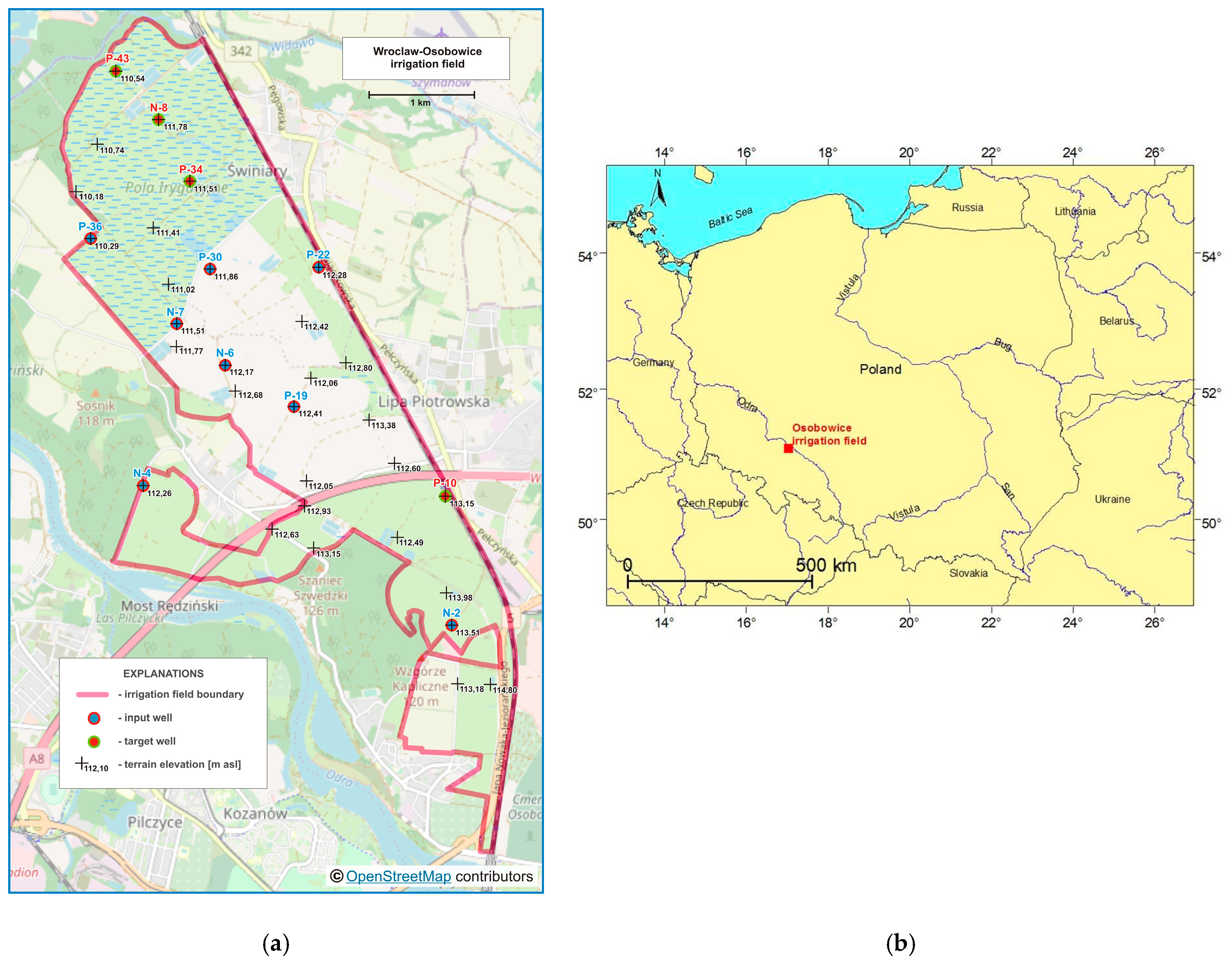
The Wrocław-Osobowice wetlands for wastewater treatment are located in the northern part of Wrocław, on the right bank of the river Odra (Figure 1a). The choice of such a location was made taking into account factors related to landforms, ownership relationships, and soil conditions. The first devices were commissioned in 1881. The exploitation started on an area of about 560 ha. It was then systematically expanded to almost 1300 ha until 2013, when water treatment usage was ended. Presently, it is an ecological area, due to the occurrence of a rich fauna and flora. As a result of ceasing flooding the fields with sewage, the amount of water supplying this area significantly decreased. Preliminary analyses enable estimates that in the last years of the wetlands’ operation, the amount of sewage discharged was similar to the amount of water from atmospheric precipitation. After 2013, the total amount of water supplying this area decreased as a consequence by one-half, which contributed to the decrease in groundwater level [22].

In mid-August 2015, a fire burned several dozen hectares of the Osobowice irrigation field. Twenty-one fire brigades and two planes fought the fire, profusely pouring water on the area. The groundwater level response to this operation was observed in three of the 12 piezometers (N-8, P-43 and P-34). For N-8, its increase was very clear (1.5 m), while for P-43 and P-34 it responded less (0.5 m and 0.02 m, respectively) because of the greater distance from the fire area. Moreover, in the period December 2015–February 2016, in P-10, the GWL fell below the measuring instrument level.

Due to the above, there was a need for reconstruction of groundwater level time series in four wells on the basis of eight neighboring areas. For this purpose, a support vector regression (SVR) method was used. GWL prediction models were created based on daily time series from neighboring wells in the period 1 May 2015–31 August 2019. The aim of the study was to evaluate the Hellwig’s method for selecting predictors (the best combinations of eight adjacent wells) for groundwater level forecasting in four other wells where data gaps were noted, using SVR models.

The main contributions of this paper are:

• The study of the performance of Hellwig’s method for selection of the predictors for groundwater level modelling;
• Daily groundwater level time series reconstruction using support vector regression models;
• Groundwater level prediction in wetlands after wastewater treatment exploitation;
• Supplementing the missing groundwater level time series.

2. Materials and Methods

2.1. Research Area

Groundwater monitoring, which provided data for the analysis contained in this work, was conducted by employees of Wrocław University of Environmental and Life Sciences on behalf of the Municipal Water and Sewage Company in Wrocław, Poland. It served to assess the water relations in the area of irrigation field in the period after termination of their exploitation as a wastewater treatment plant.

Groundwater levels were measured in a network of 31 wells in total, twelve of which were equipped with hydrostatic devices for automatic water level measurement and with recorders, saving data in nonvolatile memory, at a user-programmed time interval (every hour). In the other wells, readings were carried out with a hydrogeological whistle once a week. Only the results of measurements carried out using hydrostatic devices were used in the work. The locations of these 12 wells are shown in Figure 1a, and the location of the Osobowice irrigation field in Poland is presented in Figure 1b.

Research conducted by the Institute of Soil Science and Environmental Protection at Wrocław University of Environmental and Life Sciences showed the occurrence of alluvial soils in the analyzed area. These are mainly brown muds (in the upper layers made of clay, mainly light and medium, lined at a depth of 50–100 cm with sand or gravel) and, in lower layers, sandy muds (made of light loam sands, light loamy and strong loam sands, lined at a depth of 50–100 cm with loose sands and rarely clays). The long-term system of irrigation field exploitation, which consisted of flooding the surface of the area with wastewater rich in nutrients, did not force a deep overgrowth of plant roots deep into the profile. Shallow plants’ rooting did not favor the formation of sufficiently deep humus levels. The current methods of field exploitation, without supplying sewage, has changed the soil moisture. Permeable layers’ occurrence in the soil profile with deep groundwater levels causes water deficiency in the plants’ root zones [23].

2.2. Hellwig Method

Data from eight of the twelve wells were taken to model groundwater levels in four piezometers where data gaps were noted (in N-8, P-34, and P-43 because of fire in August 2015, whereas in P-10 because of the GWL falling below the measuring instrument level). The choice of which predictors should be used for forecasting was difficult due to the large number of possible combinations to analyze. Eight wells (N-2, N-4, N-6, N-7, P-19, P-22, P-30, P-36) located in the vicinity were used to create forecasts in piezometers N-8, P-34, P-43 and P-10, of which 255 ($S$ = 2⁸ – 1) possible combinations for each well were obtained, including single, double and triple combinations of predictors, etc., until all eight were used. Creating 255 models for each piezometer would be very work-intensive and time-consuming, and that is why the Hellwig method was used to create the rank of neighboring well combinations which served as predictors to the forecasting models. The concept is to use explanatory variables strongly dependent on the explained variable and at the same time weakly correlated with each other. However, this is not a strict criterion for the variables’ selection; in addition, there is a numerical criterion, the so-called integral capacity of information carriers’ combination. In this case, the information carriers are all explanatory variables.

For all received combinations, individual capacity of information carriers was defined according to the following formula:

$$h_j=\frac{r_j^2}{1+{{\displaystyle \sum }}_{i\ne j}\left(r_{ij}\right)}$$

(1)

where j is the variable number in the combination under consideration, r_j is the correlation coefficient of the potential explanatory variable number j with the explained variable (element of the vector of linear correlation coefficients between the explanatory variables and the explained variable R₀), and r_ij is the correlation coefficient between the ith and jth potential explanatory variables (elements of the correlation coefficients matrix between potential explanatory variables R).

H_Q measures the amount of information a variable Xj adds about variable Y in the combination. H_Q increases when r_j increases, whereas it decreases when the more variable X_j is correlated with the other explanatory variables.

The individual capacity of information carriers for all possible combination calculations of the integral capacity of information carriers was calculated according to the formula:

$$H_Q={{\displaystyle \sum }}_{j=1}^n{h}_j$$

(2)

where n is the number of predictors, j is the variable number in the combination under consideration, and h_j is the individual capacity of information carriers.

The integral capacity of information carriers for combination is the sum of the individual capacities of information carriers, which are part of this combination. It is the criterion for choosing the appropriate combination of explanatory variables, and chosen is the one with the highest H_Q [18].

2.3. SVR Modelling

In the next step, for the four analyzed piezometers, with the two best combinations of predictors according to the Hellwig method, prediction models were created using support vector regression (SVR). The results were compared with the SVR models obtained for the worst combination which brought the least information, and with the model for which all eight predictors were used.

Literature mining indicates that SVM (support vector machine) is the modelling method that gives the best prediction ability, which refers to the single and combination (hybrid) of several models and techniques [9,24,25,26,27].

SVR is an element of the SVMs derived from the classical perceptron, whose constructs are artificial neural networks. Both SVM and SVR are used to try and find a hyperplane that represents the nature of the data in the best way and control whether it meets the binding requirements of correct element classification for SVM and computational error in a specific range for SVR. In comparison to many other learning methods, the aim of both SVM and SVR is not only to adapt to the learning data, but to do so in such a way that it will enable prediction of the future behavior of the modelled phenomenon in the best way possible. For SVM, to introduce nonlinearity to the model and thus to improve its ability to cope with data that are not separated in a linear way, the so-called kernel trick is used as a standard approach [28]. The non-linear nature of the data may be caught as a result of using Radial Basis Function (RBF). The RBF kernel on two samples, x and y, represented as feature vectors in some input space, is defined as [29]:

$$K\left(x,y\right)=exp\left(-\frac{\Vert x-y{\Vert }^2}{2{\sigma }^2}\right)$$

(3)

where $\Vert x-y{\Vert }^2$ is the squared Euclidean distance between the x and y vectors, and σ is a free parameter.

For SVR, the values of the co-ordinates of the vector w and the value of the absolute term b are found by solving the following optimization problem:

Minimum $\Vert w\Vert$ maintaining:

$$\{\begin{array}{c}{y}_i-\overrightarrow{w}\cdot \overrightarrow{x_i}-b\le \epsilon \\ \overrightarrow{w}\cdot \overrightarrow{x_i}+b-y_i\le \epsilon \end{array}$$

(4)

where $\Vert w\Vert$ is the length of vector w, w is the weight vector determining the hyperplane that separates points belonging to different classes, b is the absolute term determined during optimization, x_i is a set of data belonging to two classes defined by y_i variables, y_i is the actual value corresponding to the x_i input vector, and $\mathsf{\epsilon }$ is a non-optimized method parameter that defines the acceptable level of error, i.e., of the difference between the predicted values and those that exist in the learning data.

In the present research, the daily groundwater level was predicted with the use of an SVR supported by an RBF algorithm. The parameters of the SVR model that defined the width of the margin of trust and the maximum value of weight that may be determined for the given vector were: ε = 0.1 and C = 10.0 for all models. The RBF was determined by the gamma parameter γ (width of the kernel function), equaled to 0.5 and 0.33 for the best combinations of predictors, 1.0 for the worst, and 0.125 for all eight wells taken as input variables. To prevent the phenomenon of overlearning, the dataset was divided into learning (75%) and test (25%) subsets.

For comparison purposes and to evaluate the results obtained with SVR, they were compared with artificial neural network (ANN) models using the most popular multilayer perceptron (MLP) model [25]. From several created neural networks, one for each Hellwig combination corresponding to SVR models was chosen for comparison because of the best performance. Multilayer perceptron models with different architectures were created, as stated in

Table 1. Artificial neural network (ANN) model characteristics.

N-8	no. of neurons			no. of learning epochs	activation function of neurons
	input layer	hidden layer	output layer		hidden layer	output layer
N-4, P-22	2	3	1	89	tanh	logistic
N-4, P-36	2	5	1	118	tanh	exponential
N-6	1	6	1	54	tanh	tanh
all	8	9	1	9999	exponential	logistic
P-10	no. of neurons			no. of learning epochs	activation function of neurons
	input layer	hidden layer	output layer		hidden layer	output layer
N-2, N-6	2	9	1	268	tanh	tanh
N-2, N-6, P-30	3	10	1	212	tanh	tanh
N-4	1	8	1	174	tanh	tanh
all	8	11	1	286	logistic	exponential
P-34	no. of neurons			no. of learning epochs	activation function of neurons
	input layer	hidden layer	output layer		hidden layer	output layer
N-4, P-22, P-36	3	7	1	159	tanh	tanh
N-4, P-22, P-30, P-36	4	10	1	233	tanh	exponential
N4	1	6	1	294	logistic	linear
all	8	11	1	195	tanh	logistic
P-43	no. of neurons			no. of learning epochs	activation function of neurons
	input layer	hidden layer	output layer		hidden layer	output layer
P-22, P-30, P-36	3	6	1	122	exponential	logistic
P-22, P-36	2	8	1	161	logistic	tanh
N4	1	2	1	68	logistic	linear
all	8	5	1	280	logistic	exponential

.

2.4. Models’ Quality Metrics

Models’ performance was assessed in both subsets based on the value of squared correlation (r²) for the actual and prognosed values, root mean squared error (RMSE), as well as mean absolute error (MAE) of the models according to the following formulas. Modelling was carried out using the MATLAB and Statistica programs.

$$r^2={\left(\frac{{{\displaystyle \sum }}_{i=1}^n\left(x_i-\overline{x}\right)\left(y_i-\overline{y}\right)}{\sqrt{{{\displaystyle \sum }}_{i=1}^n{\left(x_i-\overline{x}\right)}^2{{\displaystyle \sum }}_{i=1}^n{\left(y_i-\overline{y}\right)}^2}}\right)}^2$$

(5)

$$RMSE=\sqrt{\frac{1}{n}{{\displaystyle \sum }}_{i=1}^n{\left(x_i-y_i\right)}^2}$$

(6)

$$MAE=\frac{{{\displaystyle \sum }}_{i=1}^n\lceil x_i-y_i\rceil }{n}$$

(7)

where n is the number of observations, x_i are the predicted data, and y_i are the observed data.

The greater the differences between the actual and predicted values were, the greater the error was, and more adjustment was required by the network [30].

3. Results and Discussion

Table 2. Support vector regression (SVR) modelling results.

N-8	N-4, P-22			N-4, P-36			N-6			All
	learning	testing	both	learning	testing	both	learning	testing	both	learning	testing	both
RMSE	0.112	0.114	0.113	0.119	0.117	0.119	0.180	0.186	0.182	0.104	0.103	0.104
MAE	0.061	0.060	0.061	0.065	0.065	0.065	0.138	0.145	0.140	0.047	0.051	0.048
r2	0.732	0.710	0.716	0.691	0.722	0.699	0.310	0.313	0.311	0.758	0.774	0.763
P-10	N-2, N-6			N-2, N-6, P-30			N-4			all
	learning	testing	both	learning	testing	both	learning	testing	both	learning	testing	both
RMSE	0.092	0.099	0.094	0.088	0.099	0.090	0.283	0.292	0.285	0.047	0.049	0.047
MAE	0.073	0.077	0.074	0.067	0.073	0.068	0.210	0.213	0.210	0.037	0.038	0.037
r2	0.919	0.910	0.917	0.929	0.913	0.925	0.139	0.142	0.140	0.978	0.977	0.977
P-34	N-4, P-22, P-36			N-4, P-22, P-30, P-36			N-4			all
	learning	testing	both	learning	testing	both	learning	testing	both	learning	testing	both
RMSE	0.028	0.029	0.028	0.026	0.028	0.026	0.134	0.138	0.135	0.022	0.024	0.023
MAE	0.022	0.022	0.022	0.021	0.022	0.021	0.116	0.120	0.117	0.017	0.017	0.017
r2	0.980	0.980	0.980	0.981	0.980	0.981	0.562	0.565	0.564	0.986	0.986	0.986
P-43	P-22, P-30, P-36			P-22, P-36			N-4			all
	learning	testing	both	learning	testing	both	learning	testing	both	learning	testing	both
RMSE	0.072	0.080	0.074	0.080	0.087	0.081	0.200	0.214	0.204	0.051	0.056	0.053
MAE	0.058	0.064	0.060	0.064	0.070	0.066	0.163	0.175	0.166	0.041	0.044	0.042
r2	0.890	0.877	0.886	0.890	0.875	0.886	0.110	0.084	0.103	0.939	0.936	0.938

RMSE—root mean squared error MAE—mean absolute error.

contains GWL modelling results in the analyzed wells. The following lines present the values of squared correlation (r²) between the observed and predicted time series and the size of models’ errors (RMSE, MAE). In columns, the results of modelling in the learning, testing and in both samples together for the two best combinations of predictors, selected by the Hellwig method, for the combination considered the least informative, and for the model based on all eight predictors are placed.

The weakest modelling results were obtained for N-8. For the best predictor combination, according to the Hellwig method as well as for all eight predictors, r² in the testing subset equaled 0.710–0.774, whereas RMSE was 0.103–0.117 m. For N-8, the best combinations of predictors were two-element combinations N-4, P-22 and N-4, P-36. Results indicated that the least informative combination was a single piezometer N-6, which was also justified by the analysis of the correlation between groundwater levels in N-8 and in particular, individual wells (

Table 3. Correlation coefficients between response variables and their predictors.

Predictors	Response Variables
	N-8	P-10	P-34	P-43
N-2	0.5919	0.8420	0.7750	0.6061
N-4	0.7472	0.3637	0.7502	0.3608
N-6	0.4817	0.8710	0.7877	0.8220
N-7	0.6089	0.8447	0.8805	0.8913
P-19	0.6747	0.8052	0.9171	0.8056
P-22	0.6868	0.7697	0.9332	0.9135
P-30	0.6338	0.8418	0.9088	0.9158
P-36	0.6989	0.7148	0.9200	0.9099

). In N-8, it was correlated the least with N-6 and N-2 (r equaled 0.4817 and 0.5919, respectively), and the most with N-4, although r was 0.7472. That was the well with the largest response to the firefighting action in August 2015, and therefore the measurement results differed the most from the other piezometers, which was also confirmed by the forecasting results.

GWL at P-10 was predicted with RMSE in the testing subset from 0.049 to 0.099 m for all eight explanatory variables and for two combinations of predictors selected as the best by the Hellwig method (N-2, N-6 and N-2, N-6, P-30). Squared r² correlations in these cases were 0.910–0.977 for the testing sets. Groundwater level forecasting in this well, using only a single N-4 time series, provided the SVR model with the lowest quality (RMSE = 0.292 and r² = 0.142). Indeed, the measurement results in N-4 were the least correlated with P-10 (r = 0.3637), while the most with N-6 (r = 0.8710) (Table 3).

In the case of P-34, the number of elements in combination with gathering explanatory variables, considered as the best, was larger—they were sets of three (N-4, P-22, P-36) and four elements (N-4, P-22, P-30, P-36). The quality of the forecasting models created on their basis and on the basis of all eight predictors, determined by r² and RMSE, was the highest among all those analyzed (0.980–0.986; 0.024–0.029, respectively). The correlation between GWL in P-34 and time series from individual wells was also relatively high, r equaled from 0.7502 to 0.932 (Table 3). The lowest value was obtained in the case of N-4 and the highest for P-22, which was explained by the different distance between piezometers (Figure 1a).

GWL time series in P-43 were forecasted with an accuracy of 0.875–0.936 (r²) and 0.056–0.087 (RMSE) in the testing subsets for a combination based on all eight predictors and for the best combination according to Hellwig method: P-22, P-30, P-36 and P-22, P-36. Groundwater level time series from N-4 added the least amount of information to the prediction model and the correlation coefficient between N-4 and P-43 was 0.3608, while for P-36 and P-43 it was 0.9099 (Table 3). The model’s performance (created on the basis of the time series from a single N-4) was very weak: r² = 0.084 and RMSE = 0.214.

In all analyzed cases, the results of GWL measurements in individual neighboring wells, relatively away from the well for which the forecast was made, were insufficient to create a prediction model of high quality. However, the results were consistent with the statement that a unique and individual approach for a single well was needed as the model suitable for one might not necessarily be good for neighboring points [6].

It should be emphasized that the use of all eight predictors for modelling provided predictive models of higher quality than the predictors’ combinations selected as the best by Hellwig’s method. Out of the 255 possible cases, for N-8 it was 116th, for P-10, 105th, 82nd for P-34, and the 114th combination in turn for P-43. This observation required verification in additional research.

Modern approaches to groundwater level prediction, based on computational intelligence methods, have resulted in improving the models’ performance and minimization of error volume. The comparison of the results obtained with the use of the proposed method with the findings discussed in the subject literature demonstrated that the two-stage approach to daily GWL time series prediction of the combined variables selection technique with SVR is reasonable and brings the expected results. However, using the Hellwig method for this purpose needs more research. Moreover, compared to the results presented below, which concern the similar models’ performance, the quality of the created models might be considered as high (RMSE amounted to 0.024–0.292 m in the testing subset).

Wu et al. [13] demonstrated that a model combining signal decomposition (VMD) with feature extraction (Boruta) and extreme learning machine (VMD–Boruta–ELM) called VBELM generates predictions with r² = 0.8 and RMSE of 0.2–0.6. Zhao et al. [15] demonstrated that in the case of a CART model, MAE was 0.28 (in the present research MAE was 0.017–0.213). Ibrahem Ahmed Osman et al. [17] predicted GWL with performance described by the RMSE from 0.1 to 0.8, while Iqbal et al. [16] predicted 0.05. Sahoo et al. [8] obtained hybrid models of performance of 0.32–0.65 (r²) and 0.52–1.77 (RMSE), and Sharafati et al. [12] acquired values of r² = 0.66–0.94.

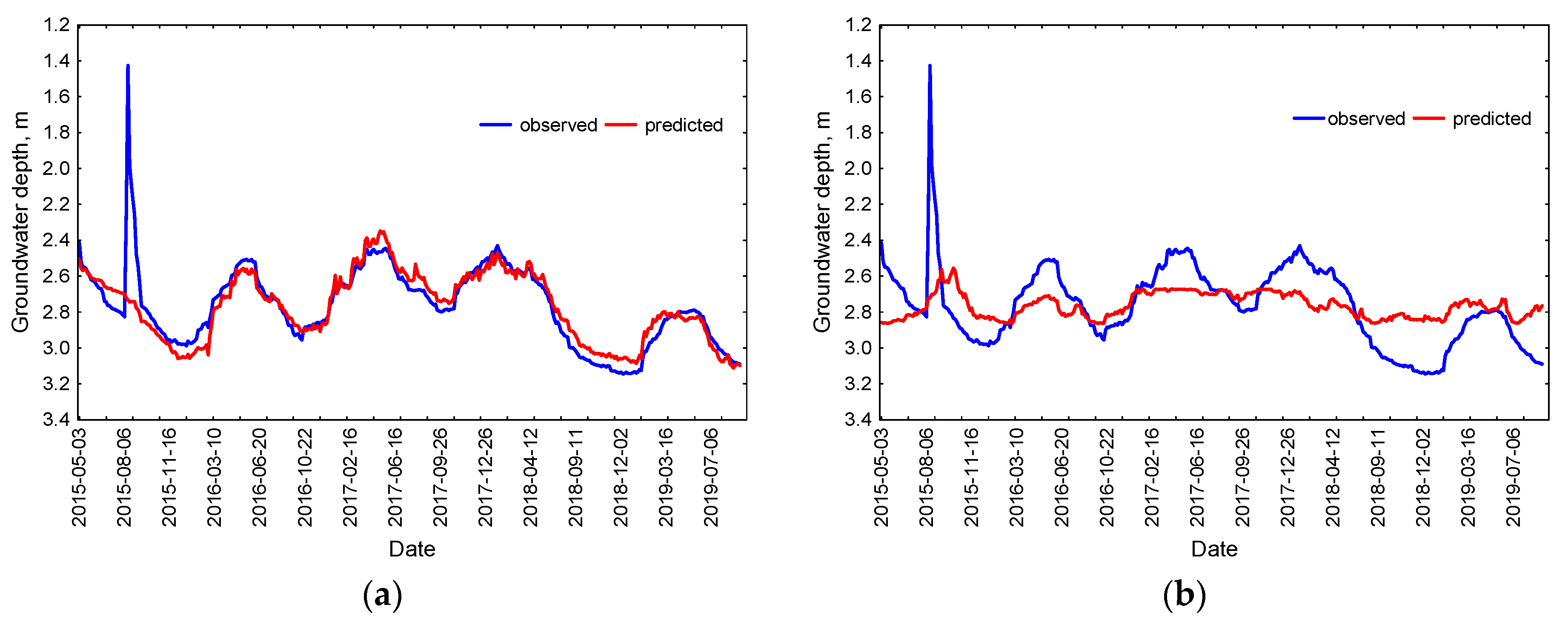
Due to the limited volume of the paper, the modelling results in graphic form were given only for the N-8 well, for which the highest increase in groundwater level was observed as a result of fire fighting in August 2015. Figure 2, Figure 3 and Figure 4 summarize the results of GWL time series forecasting (for the testing sample) in N-8 for the best (a) and worst (b) combination of predictors selected by the Hellwig method. It was found that the model for N-8, obtained on the basis of GWL time series from N-4 and P-22, reflected the reality well, although it was misleading to obtain a relatively low coefficient of determination equaled to 0.710. This was due to the fact that the model did not match the peak of August 2015, which was intentional, because it was not the result of precipitation and had to be eliminated to recreate the natural course of the time series (Figure 2a). In addition, outliers were clearly visible in Figure 3a, which was also related to the situation in August 2015. The residual histogram indicates that most numerous (190 and 170, respectively) were the differences between observed and predicted values in the range (0.0; −0.1) and (−0.1; −0.2), and extreme differences were associated with underestimation of the model in the period after the fire (Figure 4a).

In contrast to Emamgholizadeh et al. [31], Wang et al. [32] and Wunsh et al. [33] found an underestimation of high and overestimation of low GWL values; the scatter plot for N-8 presents exactly the opposite result. However, the observed under- and overestimations were minor, and they did not indicate the necessity of data divisions into low and high clusters.

The obtained results showed that the single time series coming from N-6 carried insufficient information for modelling the groundwater level in N-8 (Figure 2, Figure 3 and Figure 4b).

To evaluate SVR results, they were compared with ANN multilayer perceptron models. Results obtained with MLP models were even better than those obtained with SVR. RMSE values for the best combinations suggested by Hellwig method and for all input variables equaled from 0.010 to 0.093 (learning and testing subsets), while r² results were 0.778–0.997 (

Table 4. ANN modelling results.

N-8	N-4, P-22			N-4, P-36			N-6			All
	MLP 2-3-1			MLP 2-5-1			MLP 1-6-1			MLP 8-9-1
	learning	testing	both	learning	testing	both	learning	testing	both	learning	testing	both
RMSE	0.093	0.061	0.078	0.103	0.066	0.087	0.170	0.144	0.158	0.030	0.034	0.032
MAE	0.052	0.047	0.050	0.054	0.047	0.051	0.121	0.118	0.120	0.018	0.020	0.019
r2	0.821	0.910	0.866	0.778	0.884	0.831	0.394	0.439	0.417	0.981	0.970	0.976
P-10	N-2, N-6			N-2, N-6, P-30			N-4			all
	MLP 2-9-1			MLP 3-10-1			MLP 1-8-1			MLP 8-11-1
	learning	testing	both	learning	testing	both	learning	testing	both	learning	testing	both
RMSE	0.057	0.056	0.057	0.045	0.046	0.045	0.277	0.267	0.272	0.021	0.021	0.021
MAE	0.042	0.042	0.042	0.034	0.034	0.034	0.213	0.207	0.210	0.015	0.015	0.015
r2	0.965	0.962	0.964	0.978	0.976	0.977	0.180	0.161	0.170	0.995	0.995	0.995
P-34	N-4, P-22, P-36			N-4, P-22, P-30, P-36			N-4			all
	MLP 3-7-1			MLP 4-10-1			MLP 1-6-1			MLP 8-11-1
	learning	testing	both	learning	testing	both	learning	testing	both	learning	testing	both
RMSE	0.022	0.021	0.022	0.021	0.019	0.020	0.123	0.116	0.120	0.012	0.010	0.011
MAE	0.016	0.016	0.016	0.015	0.014	0.014	0.108	0.101	0.104	0.007	0.007	0.007
r2	0.987	0.987	0.987	0.988	0.990	0.989	0.583	0.601	0.592	0.996	0.997	0.997
P-43	P-22, P-30, P-36			P-22, P-36			N-4			all
	MLP 3-6-1			MLP 2-8-1			MLP 1-2-1			MLP 8-5-1
	learning	testing	both	learning	testing	both	learning	testing	both	learning	testing	both
RMSE	0.059	0.060	0.060	0.065	0.068	0.067	0.193	0.188	0.191	0.036	0.034	0.035
MAE	0.047	0.049	0.048	0.051	0.052	0.051	0.161	0.154	0.157	0.026	0.028	0.027
r2	0.924	0.913	0.918	0.906	0.888	0.897	0.182	0.150	0.166	0.972	0.971	0.972

).

4. Conclusions

Due to the complex nature of groundwater systems, the prediction of its behavior is a complicated task that requires complex methods. Among them, data-driven models using computational intelligence techniques are becoming increasingly popular and have significant potential because they are an alternative for multidimensional physics-based models. Moreover, CI groundwater level forecasting constitutes a modern approach to supporting groundwater management and planning. In the present research, SVR, which is part of the CI method, was used to reconstruct the incomplete time series of wells located in Wrocław-Osobowice wetlands for wastewater treatment, Poland, on the basis of the measurement period: May 1, 2015–August 31, 2019. This study aimed to evaluate the Hellwig method and input select variables. To the best of the author’s knowledge, this study is the first attempt of Hellwig method application for GWL time series implemented with an SVR model in order to find the best combination of predictors and to improve the prediction quality.

Results showed that the use of all eight predictors (wells) for modelling provided predictive models of higher quality than the predictors’ combinations selected as the best by Hellwig’s method. Out of the 255 possible cases, for N-8, it was 116th; for P-10, 105th; 82nd for P-34; and the 114th combination in turn for P-43. Those ambiguous result indicated that more research should be devoted to that area because this observation required verification in additional research.

It seems that the obtained RMSE values for the created models that equaled 0.024–0.292 m and r² of 0.7–0.9, might be subjectively considered as acceptable in the field of regional hydrology. Moreover, the created models worked well and showed good prediction ability for high as well as low daily groundwater values. Nevertheless, the comparison with MLP predictions proved to be even more accurate and led to the creation of models with better quality.

Moreover, data originated from a single well located relatively far from the analyzed piezometer are insufficient to create forecasts of high quality. Additionally, selecting the optimal input variables plays a crucial role in GWL time series reconstruction.

Additionally, the proposed method is simple, and its implementation requires access only to groundwater level measurement data. It may be useful in groundwater management and planning in terms of actual climate change and the threat of water deficits. In future studies, the authors are planning to complement the research with GWL predictions on the basis of meteorology data.

References

- Liu, D.; Li, G.; Fu, Q.; Li, M.; Liu, C.; Faiz, M.A.; Khan, M.I.; Li, T.; Cui, S. Application of Particle Swarm Optimization and Extreme Learning Machine Forecasting Models for Regional Groundwater Depth Using Nonlinear Prediction Models as Preprocessor. J. Hydrol. Eng. 2018, 23, 04018052. [Google Scholar] [CrossRef]
- Xu, T.; Valocchi, A.J.; Choi, J.; Amir, E. Use of Machine Learning Methods to Reduce Predictive Error of Groundwater Models. Ground Water 2013, 52, 448–460. [Google Scholar] [CrossRef]
- Yadav, B.; Ch, S.; Mathur, S.; Adamowski, J. Assessing the suitability of extreme learning machines (ELM) for groundwater level prediction. J. Water Land Dev. 2017, 32, 103–112. [Google Scholar] [CrossRef]
- Alsumaiei, A.A. A Nonlinear Autoregressive Modeling Approach for Forecasting Groundwater Level Fluctuation in Urban Aquifers. Water 2020, 12, 820. [Google Scholar] [CrossRef] [Green Version]
- Smarra, F.; Jain, A.; Mangharam, R.; D’Innocenzo, A. Data-driven Switched Affine Modeling for Model Predictive Control. IFAC-PapersOnLine 2018, 51, 199–204. [Google Scholar] [CrossRef]
- Sivapragasam, C.; Kannabiran, K.; Karthik, G.; Raja, S.N. Assessing Suitability of GP Modeling for Groundwater Level. Aquat. Procedia 2015, 4, 693–699. [Google Scholar] [CrossRef]
- Quilty, J.; Adamowski, J.; Khalil, B.; Rathinasamy, M. Bootstrap rank-ordered conditional mutual information (broCMI): A nonlinear input variable selection method for water resources modeling. Water Resour. Res. 2016, 52, 2299–2326. [Google Scholar] [CrossRef] [Green Version]
- Sahoo, S.; Russo, T.A.; Elliott, J.; Foster, I. Machine learning algorithms for modeling groundwater level changes in agricultural regions of the U.S. Water Resour. Res. 2017, 53, 3878–3895. [Google Scholar] [CrossRef]
- Jalalkamali, A.; Sedghi, H.; Manshouri, M. Monthly groundwater level prediction using ANN and neuro-fuzzy models: A case study on Kerman plain, Iran. J. Hydroinform. 2010, 13, 867–876. [Google Scholar] [CrossRef] [Green Version]
- Vu, M.; Jardani, A.; Massei, N.; Fournier, M. Reconstruction of missing groundwater level data by using Long Short-Term Memory (LSTM) deep neural network. J. Hydrol. 2020, 125776, 125776. [Google Scholar] [CrossRef]
- Shiri, J.; Kişi, Ö. Comparison of genetic programming with neuro-fuzzy systems for predicting short-term water table depth fluctuations. Comput. Geosci. 2011, 37, 1692–1701. [Google Scholar] [CrossRef]
- Sharafati, A.; Asadollah, S.B.H.S.; Neshat, A. A new artificial intelligence strategy for predicting the groundwater level over the Rafsanjan aquifer in Iran. J. Hydrol. 2020, 591, 125468. [Google Scholar] [CrossRef]
- Wu, M.; Feng, Q.; Wen, X.; Yin, Z.; Yang, L.; Sheng, D. Deterministic Analysis and Uncertainty Analysis of Ensemble Forecasting Model Based on Variational Mode Decomposition for Estimation of Monthly Groundwater Level. Water 2021, 13, 139. [Google Scholar] [CrossRef]
- Rahman, A.S.; Hosono, T.; Quilty, J.M.; Das, J.; Basak, A. Multiscale groundwater level forecasting: Coupling new machine learning approaches with wavelet transforms. Adv. Water Resour. 2020, 141, 103595. [Google Scholar] [CrossRef]
- Zhao, Y.; Li, Y.; Zhang, L.; Wang, Q. Groundwater level prediction of landslide based on classification and regression tree. Geodesy Geodyn. 2016, 7, 348–355. [Google Scholar] [CrossRef] [Green Version]
- Iqbal, M.; Naeem, U.A.; Ahmad, A.; Rehman, H.-U.-; Ghani, U.; Farid, T. Relating groundwater levels with meteorological parameters using ANN technique. Measurement 2020, 166, 108163. [Google Scholar] [CrossRef]
- Osman, A.I.A.; Ahmed, A.N.; Chow, M.F.; Huang, Y.F.; El-Shafie, A. Extreme gradient boosting (Xgboost) model to predict the groundwater levels in Selangor Malaysia. Ain Shams Eng. J. 2021. [Google Scholar] [CrossRef]
- Hellwig, Z. On the optimal choice of predictors. In Toward a System of Quantitative Indicators of Components of Human Resources Development; Gostkowski, Z., Ed.; UNESCO: Paris, UK, 1968. [Google Scholar]
- Omiotek, Z.; Stepanchenko, O.; Wójcik, W.; Legieć, W.; Szatkowska, M. The use of the Hellwig’s method for feature selection in the detection of myeloma bone destruction based on radiographic images. Biocybern. Biomed. Eng. 2019, 39, 328–338. [Google Scholar] [CrossRef]
- Szmidt, E.; Kacprzyk, J.; Bujnowski, P. Attribute Selection via Hellwig’s Algorithm for Atanassov’s Intuitionistic Fuzzy Sets. In Computational Intelligence and Mathematics for Tackling Complex Problems. Studies in Computational Intelligence; Kóczy, L., Medina-Moreno, J., Ramírez-Poussa, E., Šostak, A., Eds.; Springer: Cham, Switzerland, 2020; Volume 819. [Google Scholar] [CrossRef]
- Wójcik-Leń, J.; Leń, P.; Mika, M.; Kryszk, H.; Kotlarz, P. Studies regarding correct selection of statistical methods for the needs of increasing the efficiency of identification of land for consolidation—A case study in Poland. Land Use Policy 2019, 87, 104064. [Google Scholar] [CrossRef]
- Łyczko, W.M. Osobowice irrigation fields—History and present time. Inżynieria Ekologiczna 2018, 19, 37–43. [Google Scholar] [CrossRef]
- Analysis of the variability of groundwater level in the Irrigation Fields in Wrocław, Wrocław University of Environmental and Life Sciences on behalf of the Municipal Water and Sewage Company in Wrocław; summary report, typescript; Wrocław University of Environmental and Life Sciences: Wrocław, Poland, 2015.
- Suryanarayana, C.; Sudheer, C.; Mahammood, V.; Panigrahi, B. An integrated wavelet-support vector machine for groundwater level prediction in Visakhapatnam, India. Neurocomputing 2014, 145, 324–335. [Google Scholar] [CrossRef]
- Aftab, S.; Ahmad, M.; Hameed, N.; Salman, M.; Ali, I.; Nawaz, Z. Rainfall Prediction in Lahore City using Data Mining Techniques. Int. J. Adv. Comput. Sci. Appl. 2018, 9, 9. [Google Scholar] [CrossRef]
- Chu, H.; Wei, J.; Li, T.; Jia, K. Application of Support Vector Regression for Mid- and Long-term Runoff Forecasting in “Yellow River Headwater” Region. Procedia Eng. 2016, 154, 1251–1257. [Google Scholar] [CrossRef] [Green Version]
- Mosavi, A.; Ozturk, P.; Chau, K.-W. Flood Prediction Using Machine Learning Models: Literature Review. Water 2018, 10, 1536. [Google Scholar] [CrossRef] [Green Version]
- Cortes, C.; Vapnik, V. Support-vector networks. Mach. Learn. 1995, 20, 273–297. [Google Scholar] [CrossRef]
- Vert, J.-P.; Tsuda, K.; Schölkopf, B. (Eds.) A Primer on Kernel Methods in Computational Biology. In Kernel Methods in Computational Biology; The MIT Press: Cambridge, UK; pp. 35–70. [CrossRef] [Green Version]
- Dell Inc. Dell Statistica (Data Analysis Software System). 2016, 13. Available online: software.dell.com (accessed on 11 March 2021).
- Emamgholizadeh, S.; Moslemi, K.; Karami, G. Prediction the Groundwater Level of Bastam Plain (Iran) by Artificial Neural Network (ANN) and Adaptive Neuro-Fuzzy Inference System (ANFIS). Water Resour. Manag. 2014, 28, 5433–5446. [Google Scholar] [CrossRef]
- Wang, X.; Liu, T.; Zheng, X.; Peng, H.; Xin, J.; Zhang, B. Short-term prediction of groundwater level using improved random forest regression with a combination of random features. Appl. Water Sci. 2018, 8, 125. [Google Scholar] [CrossRef] [Green Version]
- Wunsch, A.; Liesch, T.; Broda, S. Forecasting groundwater levels using nonlinear autoregressive networks with exogenous input (NARX). J. Hydrol. 2018, 567, 743–758. [Google Scholar] [CrossRef]
Figure 1.
Wrocław-Osobowice irrigation field: (a) location of wells; (b) location in Poland.
Figure 2.
Observed and predicted groundwater levels (GWLs) (m) with SVR time series in the N-8 well in the test subset for the best (a) and the worst (b) combination of predictors.
Figure 3.
Relationship between observed and predicted GWLs (m) with SVR time series in the N-8 well in the test subset for the best (a) and the worst (b) combination of predictors.
Figure 4.
Residual histograms of predicted GWLs (m) with SVR time series in the N-8 well in the test subset for the best (a) and the worst (b) combination of predictors.