Modeling Transport and Adsorption of Arsenic Ions in Iron-Oxide Laden Porous Media. Part I: Theoretical Developments

Abstract

The process of transport and trapping of arsenic ions in porous water filters is treated as a classic mass transport problem which, at the pore scale, is modeled using the traditional convection-diffusion equation, representing the migration of species present in very small (tracer) amounts in water. The upscaling, conducted using the volume averaging method, reveals the presence of two possible forms of the macroscopic equations for predicting arsenic concentrations in the filters. One is the classic convection-dispersion equation with the total dispersion tensor as its main transport coefficient, and which is obtained from a closure formulation similar to that of the passive diffusion problem. The other equation form includes an additional transport coefficient, hitherto ignored in the literature and identified here as the adsorption-induced vector. These two coefficients in the latter form are determined from a system of two closure problems that include the effects of both the passive diffusion as well as the adsorption of arsenic by the solid phase of the filter. This theoretical effort represents the first serious effort to introduce a detailed micro–macro coupling while modeling the transport of arsenic species in water filters representing homogeneous porous media.

1. Introduction

The presence of arsenic in water is gravely injurious to human health. Exposure to this element leads to many skin-related, gastro-intestinal, neurological, and cardiovascular problems. Upon its consumption, the carcinogenic nature of arsenic gives rise to several types of cancers, including skin, lung and bladder cancers [1]. Contamination of water by arsenic is a problem that afflicts several parts of the world. Countries in the west, including Argentina, USA and Canada, to countries in the east, including Bangladesh, India and China, are affected by the presence of arsenic [2].

The bodies of water most affected by the problem of arsenic pollution are aquifers, which are groundwater sources. The arsenic primarily present in such sources are oxy anions with primarily two different oxidation states: arsenite (As(III)) and arsenate (As(V)) [2]. Although the arsenic can naturally dissolve into these sources of water due to its presence in the surrounding bedrock, this arsenic contamination can be exacerbated, especially in areas of Asia, through numerous human activities such as mining, smelting, using coal for power generation, and using agricultural pesticides [3].

Several water filters based on a host of separate technologies are available in the market place. These include reverse osmosis (RO), activated carbon, activated alumina, anion exchange, and distillation. Except for RO and distillation, all other methods involve forcing contaminated water to flow through a porous medium made from particles or beads. As the water comes in contact with the walls of porous media, the dissolved arsenic ions are captured by the walls through mechanisms such as anion exchange or sorption. The high surface area of porous media comes in handy for this ‘capture’. This process can be modeled with the help of a convection-diffusion equation since the extremely low concentration of arsenic in water (typically in ppb or parts-per-billion (according to the WHO guidelines, the acceptable concentration of arsenic in safe drinking water is less than 10 ppb)) allows the tracer-type species transport equations to handle the migration and absorption of this element. As a result, the modeling of arsenic transport and capture in any off-the-shelf water filter for arsenic is quite similar to the modeling of arsenic transport and capture in groundwater. We will be taking our inspiration and methodology for solving this problem in filters from the rather well-studied problem of contamination of groundwater by arsenic (or by any other toxic heavy metal such as lead).

In the fields of environmental engineering, soil sciences, geosciences and underground hydrology, contamination of groundwater flow is a well-researched problem. The large porous bodies, made of sand or similar particulate matter lodged between layers of rocks, hold a tremendous amount of groundwater and are called aquifers. The wells are drilled into these aquifers to extract water for human consumption. These aquifers exchange water with streams, rivers and ponds and hence the contamination in these water bodies is often passed on to the aquifers. The aquifers can also be contaminated by the nuclear, chemical and other type of wastes buried underground. The contaminated water traveling through the porous aquifer can get filtered due to the ion absorption process by solid particles as well as the action of bacteria. Hence, the concentration of contaminants may change with space and time during groundwater flow. Prediction of the contamination of aquifers is a big challenge that is being addressed by scientists in several countries.

The flow of water inside aquifers is modeled using Darcy’s law, and the transport of contaminants is modeled using the convection-dispersion equation for predicting the transport and attenuation of dissolved species due to adsorption and biological activity [4]. As mentioned earlier, the physics for modeling the transport and adsorption of contaminants is exactly identical to the transport and adsorption of arsenic in a water filter. Here we will describe the work that has already been done in this area as well as the limitation of that work.

Numerous analytical solutions have been developed for modeling solute transport through fully-saturated aquifers [5,6,7,8,9,10,11,12,13,14,15,16,17]. However, there are some shortcomings associated with them. For example, the dispersion tensor is simplified without any justification—it is merely presented as a constitutive relation without any correlation with the pore-scale microstructure and the phenomena occurring therein [4]. Several times, the dispersion tensor is overly simplified after dropping the molecular diffusivity contribution [5,7,10] or simply treated as a constant [8,12,14].

On the other hand, several stochastic groundwater modeling techniques have been proposed to study the transport of solute in natural porous formations like aquifers with variable permeability [18,19,20]. Dagan [19] explained that the spatial distribution of solute in such porous structures is mostly governed by convection and the heterogeneity of permeability on a large scale. In these cases, the marginal effect of pore-scale dispersion is generally neglected owing to the smallness of the transverse dispersivity with respect to the heterogeneity scale. Aldo [20] furthered this study [19] and investigated the influence of the pore-scale dispersion mechanism in an heterogenous aquifer under both the ergodic and nonergodic transport conditions. In the same vein, Rubin [21] presented the stochastic formulations of the advection-dispersion equation to model the transport of tracer species in heterogeneous porous media. Such mathematical models are often based on the assumptions of stationarity, ergodicity, and gaussian distribution, and seek geostatistical parameters for stochastic modeling. These approaches have earned some success in correlating different length-scales and are able to predict the results of large-scale controlled field experiments [22,23]. However, they lack the ability to account for the influence of pore-level microstructural details in the formulation of the total dispersion tensor, which needs further development. In the proposed research described below, we will develop a more comprehensive analysis for species transport using a micro–macro coupling that can remove the above-mentioned shortcomings and lead to an important advance in this area.

The method of volume averaging is a rigorous method to upscale from the pore scale to the macroscopic lab or field scale [24,25,26]. The use of this method in understanding and predicting mass transport in porous media has had a long history, and a brief synopsis is presented here. One of the first attempts to understand and model diffusion and hydrodynamic dispersion in porous media can be attributed to Whitaker [27]. Gray later [28] suggested an improvement in Whitaker’s formulation by suggesting the estimation of the deviations from the intrinsic phase-average (instead of the phase-average) for the concentration of the solute. Attempts were made to understand hydrodynamic dispersion in capillary tubes representing porous media, which led to the confirmation of the Taylor-Aries model [29]. Later the same ideas were applied to develop a one-Equation [30] and a two-Equation [31] model for solute transport accompanied with adsorption in dual length-scale heterogeneous porous media. The volume averaging method was then adapted to find the effective dispersion tensor in a heterogeneous medium, the findings of which were tested using the ensemble averaging process [32]. The two-equation model was later employed to estimate the macroscopic properties of an ideal heterogenous porous medium and a parametric study was conducted to study the effect of the Péclet number, permeability ratio and local-scale dispersitivity on the dispersion coefficient [33].

In this paper, we will employ the volume averaging method to upscale the phenomenon of solute transport (which include both diffusion and advection) accompanied with adsorption in homogeneous porous media. Such media are found in commercial water filters where the cartridges created by packing particles or beads that can be assumed to be of mono-modal size distribution and thus create single-scale porous media. It may seem that the solution to this relatively simple problem should exist somewhere in the volume-averaging literature. However, the authors’ investigation revealed that bits and pieces of this problem exist piecemeal at different locations. For example, similar problems on diffusion without advection, and accompanied with adsorption, have been formulated as practice problems by Whitaker in their monograph (Problems 4 and 25 in chapter 1 of [26]). Later, solving the same problem after including the advection has been presented in Problem 13 of chapter 3 on dispersion; however, it is presented without any solution. Similarly, Plumb and Whitaker [34] presented the upscaling theory corresponding to diffusion, adsorption and advection in porous media composed of porous particles in Section 5 of [34]. This one-equation model approach was a multi-scale treatment that involved lower-scale averaging inside what will be our solid phase here.

One can cite some more of the similar developments in the volume averaging method that are related to the proposed formulation. Whitaker in chapter 1 of [35] illustrated the use of the volume averaging procedure and the boundary conditions required to derive the upscaled convective-dispersion equation with nonlinear adsorption for species transport. Wood et al. [36] developed a volume-averaged macroscale transport equation for a reactive chemical species and compared the effective reaction rate obtained from the closure formulation to that from the direct numerical simulation at the microscale. Similarly, Valdés-Parada et al. [37] carried out upscaling of mass transport equations along with diffusion and convection based reaction processes in porous media. In the same vein, the work by Quintard et al. [38,39] had some useful developments for the interfacial boundary condition for the moving-phase velocity.

Hence, the authors had to gather and develop all the relevant aspects of the upscaling physics for the considered practical problem of developing for arsenic water filters the upscaled governing equation and the associated closure problem. A researcher experienced in the volume average method may find several portions of the manuscript repetitions of what is available in the literature; however, the authors feel that all the main derivations should be presented in the paper here in order to improve its readability and bring diverse aspects into a single presentation.

2. Model for Solute Transport

2.1. Mathematical Preliminaries and Definitions

The volume averaging method will be used to upscale from the microscopic space to the macroscopic one. This means that the governing equations and boundary conditions for the large-scale space will be derived from the governing equations plus boundary conditions for the small-scale space. We will start with some basic definitions.

2.1.1. Representative Averaging Volume

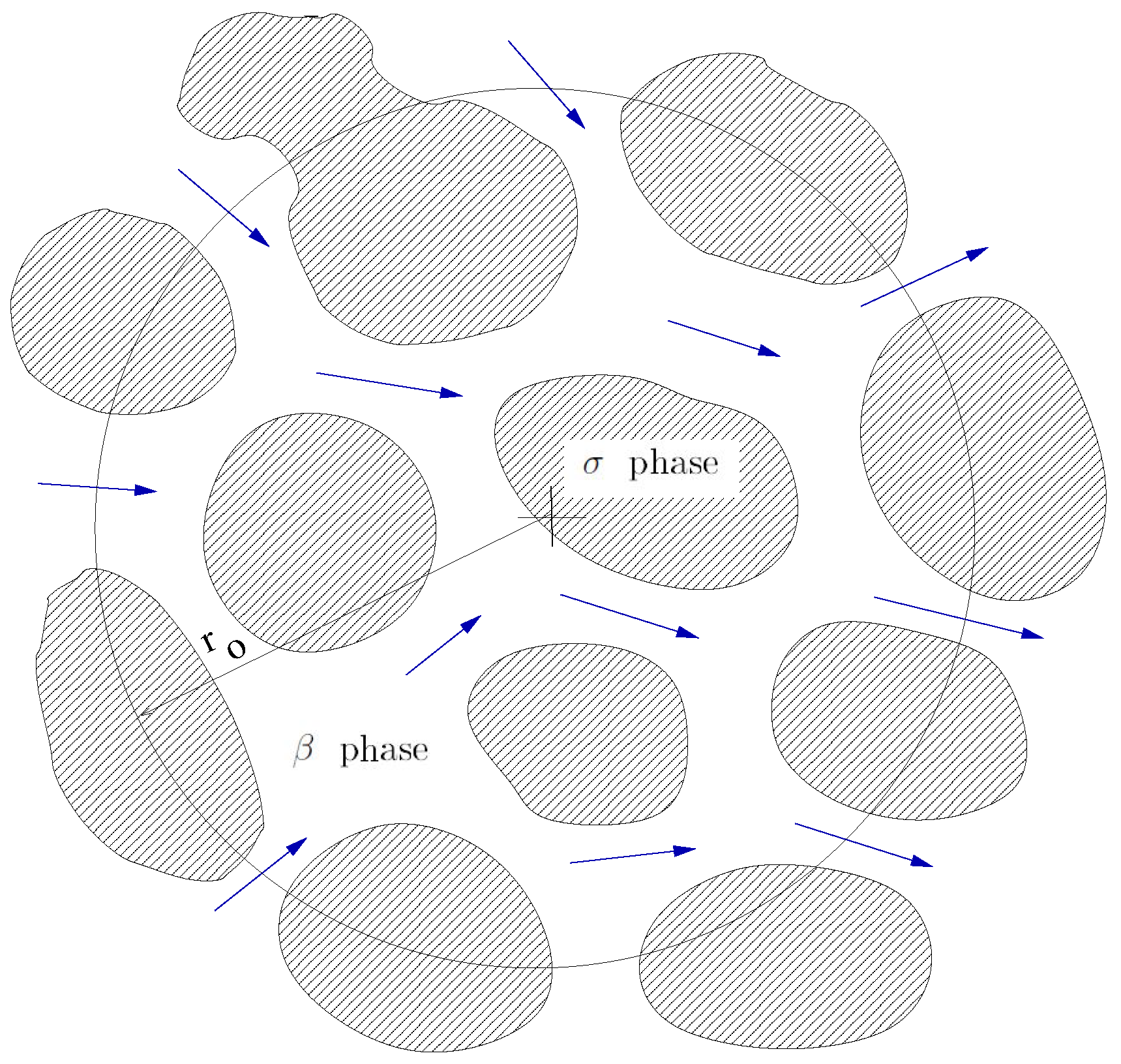
The representative elementary volume (REV) plays an important conceptual role in upscaling of porous media processes. As shown in Figure 1, it is often taken to be of a spherical form. Our problem is classified as the single-phase flow through porous media. Hence, there is a phase called $\beta$ phase that flows between the stationary, non-deforming solid particles made from the $\sigma$ phase and completely fills the pores. During this flow, the ions being carried by the flowing $\beta$ phase (water) are also moving towards the $\sigma$ phase particles and are getting adsorbed by them.

For effective volume averaging, the following constraint is required [26]:

$$\mathrm{Average} \mathrm{Particle} \mathrm{Size}\hspace{1em}<<\hspace{1em}{r}_o\hspace{1em}<<\hspace{1em}\mathrm{Size} \mathrm{of} \mathrm{the} \mathrm{upscaled} \mathrm{domain}$$

(1)

where $r_o$ is the size of the REV.

2.1.2. Phase and Intrinsic Phase Averages

The phase average $\langle {\varphi }_{\beta }\rangle$ for any variable ${\varphi }_{\beta }$ associated with the $\beta$ phase flowing through the porous medium is defined as

$$\langle {\varphi }_{\beta }\rangle = \frac{1}{V}{\int }_{V_{\beta }}{\varphi }_{\beta } dV$$

(2)

where V is the volume of the REV. $\langle {\varphi }_{\beta }\rangle$ represents the average value of any quantity within the whole of the REV.

On the other hand, there is an average called the intrinsic phase average, ${\langle {\varphi }_{\beta }\rangle }^{\beta }$, which is the average value of any quantity only within the β phase of the REV. Such an average is defined as

$${\langle {\varphi }_{\beta }\rangle }^{\beta } = \frac{1}{V_{\beta }}{\int }_{V_{\beta }}{\varphi }_{\beta } dV$$

(3)

where $V_{\beta }$ represents the volume of the $\beta$ phase within the REV.

As one can easily see, the relation between the two averages is

$$\langle {\varphi }_{\beta }\rangle = {ϵ}_{\beta } {\langle {\varphi }_{\beta }\rangle }^{\beta }$$

(4)

such that ${ϵ}_{\beta }$ is the volume fraction of the $\beta$ phase given by the relation

$${ϵ}_{\beta } = \frac{V_{\beta }}{V}$$

(5)

Note that for single-phase flow of the $\beta$ phase through our porous medium, ${ϵ}_{\beta }$ will be equal to the porosity of the porous medium, since the latter is defined as the ratio of the total pore volume within REV to the total REV volume.

2.1.3. Averaging Theorems

We will now present two important theorems that are used in the upscaling of transport and flow equations in porous media. A formal and easy to understand proof of these theorems can be found in [40], although similar proofs have been presented elsewhere [24,25,26,41].

First Averaging Theorem

This theorem relates the phase average of a gradient or a divergence of a physical quantity to the gradient or divergence of the phase average of the quantity. As before, any variable ${\varphi }_{\beta }$ associated with the $\beta$ phase flowing through the porous medium will satisfy the following relationship:

$$\langle \nabla {\varphi }_{\beta }\rangle = \nabla \langle {\varphi }_{\beta }\rangle + \frac{1}{V}{\int }_{A_{\beta \sigma }}{\varphi }_{\beta } {\mathbf{n}}_{\beta \sigma } dA$$

(6)

where ${\mathbf{n}}_{\beta \sigma }$ is the unit normal directed from $\beta$ phase to $\sigma$ phase, and $A_{\beta \sigma }$ is the interfacial area between the $\beta$ and $\sigma$ phases. In case the variable ${\varphi }_{\beta }$ is a vector, then we deal with divergence of this quantity as shown below.

$$\langle \nabla ·{\varphi }_{\beta }\rangle = \nabla ·\langle {\varphi }_{\beta }\rangle + \frac{1}{V}{\int }_{A_{\beta \sigma }}{\varphi }_{\beta }·{\mathbf{n}}_{\beta \sigma } dA$$

(7)

Second Averaging Theorem

This theorem relates the phase average of a time derivative to the time derivative of the phase average as follows:

$$\langle \frac{\partial {\varphi }_{\beta }}{\partial t}\rangle = \frac{\partial \langle {\varphi }_{\beta }\rangle }{\partial t} - \frac{1}{V}{\int }_{A_{\beta \sigma }}{\varphi }_{\beta } \mathbf{w}·{\mathbf{n}}_{\beta \sigma } dA$$

(8)

where $\mathbf{w}$ is the velocity of the $\beta -\sigma$ interface.

2.2. Upscaling by Volume Averaging Method

The governing equation for solute transport within the pore space of an REV can be expressed as

$$\frac{\partial c_{\beta }}{\partial t} + \nabla ·\left(c_{\beta }{\mathbf{v}}_{\beta }\right) = \nabla ·\left({\mathcal{D}}_{\beta }\nabla c_{\beta }\right)$$

(9)

where $c_{\beta }$ is the point concentration in the $\beta$ phase, ${\mathbf{v}}_{\beta }$ is the velocity of the $\beta$ phase, and ${\mathcal{D}}_{\beta }$ is the molecular diffusivity of the $\beta$ phase. Note that it is a tracer equation, i.e., the concentration of the transported species, $c_{\beta }$, is extremely small. This is a convection-diffusion type equation where velocity of the fluid $\beta$ phase is given (see [42] for a rigorous derivation of this equation).

Let us now specify the boundary conditions needed to solve for $c_{\beta }$ within the pore region of an REV. A flux of solute ions is created onto the $\beta -\sigma$ interface, which leads to the rate of increase in the surface concentration of the adsorbed ions. This can be expressed as $-{\mathbf{n}}_{\beta \sigma }·{\mathcal{D}}_{\beta }\nabla c_{\beta } = \frac{\partial c_{ad}}{\partial t}$, where $c_{ad}$ represents the surface concentration on the $\beta -\sigma$ interface. However, our analysis is limited to linear adsorption isotherms and local mass equilibrium exists at the $\beta -\sigma$ interface [29,30], i.e., $c_{ad} = K_{eq} c_{\beta }$. Here, $K_{eq}$ is the equilibrium coefficient (or the distribution coefficient) corresponding to the linear isotherm. On combining these two relations, the proposed boundary condition reduces to

$$\mathrm{B}.\mathrm{C}.1 :\hspace{1em}-{\mathbf{n}}_{\beta \sigma }·{\mathcal{D}}_{\beta }\nabla c_{\beta } = K_{eq}\frac{\partial c_{\beta }}{\partial t}, \hspace{1em}\mathrm{at} A_{\beta \sigma }$$

(10)

It is helpful for future analysis to state here the continuity equation for the $\beta$ phase as well as the associated no-slip boundary condition at the $\beta -\sigma$ interface:

$$\begin{array}{ccc}\hfill \nabla ·{\mathbf{v}}_{\beta } & =& 0\hfill \\ \hfill \mathrm{B}.\mathrm{C}.2 :\hspace{1em}{\mathbf{v}}_{\beta } & =& 0, \hspace{1em}\mathrm{at} A_{\beta \sigma }\hfill \end{array}$$

(11)

On taking the phase-average of Equation (9), we get

$$\langle \frac{\partial c_{\beta }}{\partial t}\rangle + \langle \nabla ·\left(c_{\beta }{\mathbf{v}}_{\beta }\right)\rangle = \langle \nabla ·\left({\mathcal{D}}_{\beta }\nabla c_{\beta }\right)\rangle$$

(12)

Let us consider the three terms of this equation one by one. On applying the second averaging theorem, the first term on the left-hand side of this equation results in

$$\langle \frac{\partial c_{\beta }}{\partial t}\rangle = \frac{\partial \langle c_{\beta }\rangle }{\partial t} - \frac{1}{V}{\int }_{A_{\beta \sigma }}{c}_{\beta } \mathbf{w}·{\mathbf{n}}_{\beta \sigma } dA = \frac{\partial \langle c_{\beta }\rangle }{\partial t}$$

(13)

The integral term involving the interface velocity $\mathbf{w}$ disappears since we have taken the porous medium to be rigid (non-deforming) and stationary. On applying the first averaging theorem, the second term on the left-hand side of Equation (12) develops as

$$\langle \nabla ·\left(c_{\beta }{\mathbf{v}}_{\beta }\right)\rangle = \nabla ·\langle c_{\beta }{\mathbf{v}}_{\beta }\rangle - \frac{1}{V}{\int }_{A_{\beta \sigma }}{c}_{\beta } {\mathbf{v}}_{\beta }·{\mathbf{n}}_{\beta \sigma } dA = \nabla ·\langle c_{\beta }{\mathbf{v}}_{\beta }\rangle$$

(14)

Here the integral term disappears because of the no-slip condition described in Equation (11).

Let us now look into the development of the term on the right-hand side of Equation (12). The application of the first averaging theorem leads to the following unfolding:

$$\begin{array}{ccc}\hfill \langle \nabla ·\left({\mathcal{D}}_{\beta }\nabla c_{\beta }\right)\rangle & =& \nabla ·\langle {\mathcal{D}}_{\beta }\nabla c_{\beta }\rangle + \frac{1}{V}{\int }_{A_{\beta \sigma }}{\mathcal{D}}_{\beta }\nabla c_{\beta }·{\mathbf{n}}_{\beta \sigma } dA\hfill \\ & =& \nabla ·\langle {\mathcal{D}}_{\beta }\nabla c_{\beta }\rangle - \frac{1}{V}{\int }_{A_{\beta \sigma }}{K}_{eq}\frac{\partial c_{\beta }}{\partial t} dA\hfill \\ & =& \nabla ·\langle {\mathcal{D}}_{\beta }\nabla c_{\beta }\rangle - K_{eq}\frac{\partial }{\partial t}[\frac{A_{\beta \sigma }}{V} \frac{1}{A_{\beta \sigma }} {\int }_{A_{\beta \sigma }}{c}_{\beta } dA]\hfill \end{array}$$

(15)

Here we use B.C.1 given in Equation (10) as well as the facts that (a) $K_{eq}$ is taken as a constant within the REV, and (b) the time derivative can be taken out of the surface integral since we are dealing with a rigid (non-deforming) porous medium that ensures that the interfacial area within the REV remains unchanged. Thus, by implementing these transformations in the interfacial-flux term within the surface integral, we are able to include the effect of adsorption into the upscaled mass-transport equation.

At this stage, we introduce two definitions:

$$\left(\mathrm{I}\right)\hspace{1em}\hspace{1em}{a}_{\beta \sigma } = \frac{A_{\beta \sigma }}{V}$$

(16)

where $A_{\beta \sigma }$ is the net $\beta -\sigma$ interfacial area contained with the REV volume, and $a_{\beta \sigma }$ is equal to the $\beta -\sigma$ interfacial area per unit volume.

$$\left(\mathrm{II}\right)\hspace{1em}\hspace{1em}{\langle c_{\beta }\rangle }_{\beta \sigma }=\frac{1}{A_{\beta \sigma }} {\int }_{A_{\beta \sigma }}{c}_{\beta } dA$$

(17)

where ${\langle c_{\beta }\rangle }_{\beta \sigma }$ is the average concentration on the interfacial area.

Through the use of these two definitions, the term on the right-hand side of Equation (11) can be expressed as

$$\langle \nabla ·\left({\mathcal{D}}_{\beta }\nabla c_{\beta }\right)\rangle =\nabla ·\langle {\mathcal{D}}_{\beta }\nabla c_{\beta }\rangle - K_{eq} a_{\beta \sigma } \frac{\partial {\langle c_{\beta }\rangle }_{\beta \sigma }}{\partial t}$$

(18)

Further employment of the first averaging theorem to the first term of the right-hand side leads to

$$\langle \nabla ·\left({\mathcal{D}}_{\beta }\nabla c_{\beta }\right)\rangle =\nabla ·\left[{\mathcal{D}}_{\beta }\left(\nabla \langle c_{\beta }\rangle + \frac{1}{V}{\int }_{A_{\beta \sigma }}{c}_{\beta } {\mathbf{n}}_{\beta \sigma } dA\right)\right] - K_{eq} a_{\beta \sigma } \frac{\partial {\langle c_{\beta }\rangle }_{\beta \sigma }}{\partial t}$$

(19)

Finally, on using Equations (13), (14) and (19) in Equation (12), we get an intermediate form of the volume-averaged solute transport equation:

$$\frac{\partial \langle c_{\beta }\rangle }{\partial t} + \nabla ·\langle c_{\beta }{\mathbf{v}}_{\beta }\rangle = \nabla ·\left[{\mathcal{D}}_{\beta }\left(\nabla \langle c_{\beta }\rangle + \frac{1}{V}{\int }_{A_{\beta \sigma }}{c}_{\beta } {\mathbf{n}}_{\beta \sigma } dA\right)\right] - K_{eq} a_{\beta \sigma } \frac{\partial {\langle c_{\beta }\rangle }_{\beta \sigma }}{\partial t}$$

(20)

We will now transform this equation in terms of the intrinsic phase-average using the relation

$$\langle c_{\beta }\rangle = {ϵ}_{\beta } {\langle c_{\beta }\rangle }^{\beta }$$

(21)

which is based on Equation (4). This results in

$$\begin{array}{ccc}\hfill {ϵ}_{\beta } \frac{\partial {\langle c_{\beta }\rangle }^{\beta }}{\partial t} + \nabla ·\langle c_{\beta }{\mathbf{v}}_{\beta }\rangle & =& \nabla ·\left[{\mathcal{D}}_{\beta }\left({ϵ}_{\beta }\nabla {\langle c_{\beta }\rangle }^{\beta } + {\langle c_{\beta }\rangle }^{\beta } \nabla {ϵ}_{\beta } + \frac{1}{V}{\int }_{A_{\beta \sigma }}{c}_{\beta } {\mathbf{n}}_{\beta \sigma } dA\right)\right] \hfill \\ & -& K_{eq} a_{\beta \sigma } \frac{\partial {\langle c_{\beta }\rangle }_{\beta \sigma }}{\partial t}\hfill \end{array}$$

(22)

Our aim is to develop an equation in terms of the macroscopic variable ${\langle c_{\beta }\rangle }^{\beta }$ entirely. However, we have some unknown terms in the equation which are preventing us from reaching this goal. These terms are the dispersion term $\langle c_{\beta }{\mathbf{v}}_{\beta }\rangle$, the surface integral term on the right-hand side, as well as the transient term involving ${\langle c_{\beta }\rangle }_{\beta \sigma }$. Hence some more work lies ahead of us.

In order to proceed further, we will take the help of the following well-known decompositions

$$c_{\beta } = {\langle c_{\beta }\rangle }^{\beta } + {\tilde{c}}_{\beta }\hspace{1em}\mathrm{and}\hspace{1em}{\mathbf{v}}_{\beta } = {\langle {\mathbf{v}}_{\beta }\rangle }^{\beta } + {\tilde{\mathbf{v}}}_{\beta }$$

(23)

where ${\langle c_{\beta }\rangle }^{\beta }$ is the intrinsic phase-average concentration in the $\beta$ phase and ${\tilde{c}}_{\beta }$ is the spatial deviation in concentration of the $\beta$ phase. Similarly, ${\langle {\mathbf{v}}_{\beta }\rangle }^{\beta }$ is the intrinsic phase-average velocity in the $\beta$ phase and ${\tilde{\mathbf{v}}}_{\beta }$ is the spatial deviation in velocity of the $\beta$ phase.

This is essentially a splitting of length scales with ${\langle c_{\beta }\rangle }^{\beta }$ varying over a much larger length-scale, say $l_{{\langle c_{\beta }\rangle }^{\beta }}$ while ${\tilde{c}}_{\beta }$ varying over the characteristic length $l_{{\tilde{c}}_{\beta }}$. Here the constraint associated with this splitting [26] is

$$l_{{\tilde{c}}_{\beta }} << r_o << l_{{\langle c_{\beta }\rangle }^{\beta }}$$

(24)

with $r_o$ being the size of the REV. This constraint allows one to treat the average ${\langle c_{\beta }\rangle }^{\beta }$ as a constant in the volume and area integrals within the REV. A similar set of constraints and conclusions can be associated with the decomposition associated with velocity given in Equation (23). Using the property of these averages to be constant within the REV, it is easy to prove the following corollary associated with the decomposition, i.e.,

$$\langle {\tilde{c}}_{\beta }\rangle = 0\hspace{1em}\mathrm{and}\hspace{1em}\langle {\tilde{\mathbf{v}}}_{\beta }\rangle = 0$$

(25)

Through the use of Equations (23) and (25), the dispersion term of Equation (22) can be transformed as

$$\begin{array}{ccc}\hfill \langle c_{\beta }{\mathbf{v}}_{\beta }\rangle & =& \langle {\langle c_{\beta }\rangle }^{\beta }{\langle {\mathbf{v}}_{\beta }\rangle }^{\beta }\rangle + \langle {\langle c_{\beta }\rangle }^{\beta }{\tilde{\mathbf{v}}}_{\beta }\rangle + \langle {\tilde{c}}_{\beta }{\langle {\mathbf{v}}_{\beta }\rangle }^{\beta }\rangle + \langle {\tilde{c}}_{\beta }{\tilde{\mathbf{v}}}_{\beta }\rangle \hfill \\ & =& {\langle c_{\beta }\rangle }^{\beta }{\langle {\mathbf{v}}_{\beta }\rangle }^{\beta }{ϵ}_{\beta } + 0 + 0 + \langle {\tilde{c}}_{\beta }{\tilde{\mathbf{v}}}_{\beta }\rangle \hfill \\ & =& {ϵ}_{\beta }{\langle c_{\beta }\rangle }^{\beta }{\langle {\mathbf{v}}_{\beta }\rangle }^{\beta } + {ϵ}_{\beta }{\langle {\tilde{c}}_{\beta }{\tilde{\mathbf{v}}}_{\beta }\rangle }^{\beta }\hfill \end{array}$$

(26)

In these derivations, we have also used the relation between the phase-average and the intrinsic phase-average as given by Equation (21), as well as the fact that $\langle 1\rangle ={ϵ}_{\beta }$ which follows from the basic definitions given earlier in Equations (2) and (5). Using the continuity equation given in Equation (11), the divergence of the dispersion term can be expressed as

$$\nabla ·\langle c_{\beta }{\mathbf{v}}_{\beta }\rangle = {ϵ}_{\beta }{\langle {\mathbf{v}}_{\beta }\rangle }^{\beta }·\nabla {\langle c_{\beta }\rangle }^{\beta } + \nabla ·\left({ϵ}_{\beta }{\langle {\tilde{c}}_{\beta }{\tilde{\mathbf{v}}}_{\beta }\rangle }^{\beta }\right)$$

(27)

Let us now consider the surface integral term on the right-hand side of Equation (22). If we use the result $\left(\nabla {ϵ}_{\beta }\right)=-\frac{1}{V}{\int }_{A_{\beta \sigma }}{\mathbf{n}}_{\beta \sigma } {\tilde{c}}_{\beta } dA$, which is obtained after substituting ${\varphi }_{\beta }=1$ in the first averaging theorem (Equation (6)), in conjunction with the decomposition given in Equation (23), we get the following result:

$$\begin{array}{ccc}\hfill \frac{1}{V}{\int }_{A_{\beta \sigma }}{\mathbf{n}}_{\beta \sigma } c_{\beta } dA& =& \left(\frac{1}{V}{\int }_{A_{\beta \sigma }}{\mathbf{n}}_{\beta \sigma } dA\right){\langle c_{\beta }\rangle }^{\beta } + \frac{1}{V}{\int }_{A_{\beta \sigma }}{\mathbf{n}}_{\beta \sigma } {\tilde{c}}_{\beta } dA\hfill \\ & =& -\left(\nabla {ϵ}_{\beta }\right){\langle c_{\beta }\rangle }^{\beta } + \frac{1}{V}{\int }_{A_{\beta \sigma }}{\mathbf{n}}_{\beta \sigma } {\tilde{c}}_{\beta } dA\hfill \end{array}$$

(28)

Let us now try to exploit the developments in these last two equations in order to get closer to our goal of developing a macroscopic governing equation only in terms of the macroscopic average terms. On using the results of Equations (27) and (28) in Equation (22), we get

$$\begin{array}{cc}\hfill {ϵ}_{\beta } \frac{\partial {\langle c_{\beta }\rangle }^{\beta }}{\partial t} & + {ϵ}_{\beta }{\langle {\mathbf{v}}_{\beta }\rangle }^{\beta }·\nabla {\langle c_{\beta }\rangle }^{\beta } + \nabla ·\left({ϵ}_{\beta }{\langle {\tilde{c}}_{\beta }{\tilde{\mathbf{v}}}_{\beta }\rangle }^{\beta }\right) \hfill \\ \hfill \hspace{1em}& = \nabla ·\left[{\mathcal{D}}_{\beta }\left({ϵ}_{\beta }\nabla {\langle c_{\beta }\rangle }^{\beta } + \frac{1}{V}{\int }_{A_{\beta \sigma }}{\mathbf{n}}_{\beta \sigma } {\tilde{c}}_{\beta } dA\right)\right] - K_{eq} a_{\beta \sigma } \frac{\partial {\langle c_{\beta }\rangle }_{\beta \sigma }}{\partial t}\hfill \end{array}$$

(29)

In this equation, we can notice the mathematical representations of the different transport mechanisms involved. On the left-hand side of Equation (29), the first term accounts for accumulation of the tracer species, the second term corresponds to the convective flux, and the third term captures the hydrodynamic dispersion phenomenon, which, as widely accepted [43], is the result of spatial deviations in the pore-level velocity field. Similarly, on the right-hand side of the equation, the first term represents the diffusive flux originating due to spatial gradient of the average concentration, and the macrodiffusive or non-local diffusive flux based on perturbations in the concentration field, whereas the last term accounts for the adsorptive flux onto the $\beta -\sigma$ interfacial surface. It should be noted that porous media have significantly high specific interfacial area (i.e., large $A_{\beta \sigma }$ within the REV) which makes them highly effective for adsorption-based applications, and in this case, may also make the adsorptive-flux term significant even in the cases with small rates of change of average concentration.

Let us now work on the transient term on the left-hand side of Equation (29). In view of the constraints expressed by Equation (24), and according to [34], it is acceptable to use the following approximations:

$${\langle {\langle c_{\beta }\rangle }^{\beta }\rangle }_{\beta \sigma } = {\langle c_{\beta }\rangle }^{\beta }\hspace{1em}\mathrm{and}\hspace{1em}{\langle {\tilde{c}}_{\beta }\rangle }_{\beta \sigma } = 0$$

(30)

The use of Equation (23) in the transient term along with these approximations allows one to rewrite Equation (29) in a simplified form:

$$\begin{array}{r}{ϵ}_{\beta } \left(1 + \frac{K_{eq}{a}_{\beta \sigma }}{{ϵ}_{\beta }}\right)\frac{\partial {\langle c_{\beta }\rangle }^{\beta }}{\partial t} + {ϵ}_{\beta }{\langle {\mathbf{v}}_{\beta }\rangle }^{\beta }·\nabla {\langle c_{\beta }\rangle }^{\beta }\\ = \nabla ·\left[{ϵ}_{\beta }{\mathcal{D}}_{\beta }\left(\nabla {\langle c_{\beta }\rangle }^{\beta } + \frac{1}{V_{\beta }}{\int }_{A_{\beta \sigma }}{\mathbf{n}}_{\beta \sigma } {\tilde{c}}_{\beta } dA\right)\right]\\ - \nabla ·\left({ϵ}_{\beta }{\langle {\tilde{c}}_{\beta }{\tilde{\mathbf{v}}}_{\beta }\rangle }^{\beta }\right)\end{array}$$

(31)

2.3. Seeking Closure

In order to estimate the unknown terms in Equation (31) involving ${\tilde{c}}_{\beta }$, we plan to propose a set of equations for the same. Later, those equations will be transformed in order to obtain what is called the closure formulation.

We start with Equation (9), where, after using the decomposition given in Equation (23), we obtain:

$$\begin{array}{ccc}\hfill \frac{\partial {\langle c_{\beta }\rangle }^{\beta }}{\partial t} + \frac{\partial {\tilde{c}}_{\beta }}{\partial t} & +& \nabla ·\left({\langle c_{\beta }\rangle }^{\beta }{\langle {\mathbf{v}}_{\beta }\rangle }^{\beta }\right) + \nabla ·\left({\langle c_{\beta }\rangle }^{\beta }{\tilde{\mathbf{v}}}_{\beta }\right) + \nabla ·\left({\tilde{c}}_{\beta }{\langle {\mathbf{v}}_{\beta }\rangle }^{\beta }\right) + \nabla ·\left({\tilde{c}}_{\beta }{\tilde{\mathbf{v}}}_{\beta }\right)\hfill \\ & =& \nabla ·({\mathcal{D}}_{\beta }\nabla {\langle c_{\beta }\rangle }^{\beta }) + \nabla ·({\mathcal{D}}_{\beta }\nabla {\tilde{c}}_{\beta })\hfill \end{array}$$

(32)

On dividing Equation (31) with ${ϵ}_{\beta }$ and rearranging the terms, we get

$$\begin{array}{cc}\hfill \left(1 + \frac{K_{eq}{a}_{\beta \sigma }}{{ϵ}_{\beta }}\right)\frac{\partial {\langle c_{\beta }\rangle }^{\beta }}{\partial t} & + {\langle {\mathbf{v}}_{\beta }\rangle }^{\beta }·\nabla {\langle c_{\beta }\rangle }^{\beta }+ {ϵ}_{\beta }^{-1} \nabla ·\langle {\tilde{c}}_{\beta }{\tilde{\mathbf{v}}}_{\beta }\rangle \hfill \\ \hfill \hspace{1em}& = {ϵ}_{\beta }^{-1} \nabla ·({ϵ}_{\beta } {\mathcal{D}}_{\beta } \nabla {\langle c_{\beta }\rangle }^{\beta }) + {ϵ}_{\beta }^{-1} \nabla ·\left[{\mathcal{D}}_{\beta }\left(\frac{1}{V}{\int }_{A_{\beta \sigma }}{\mathbf{n}}_{\beta \sigma } {\tilde{c}}_{\beta } dA\right)\right]\hfill \end{array}$$

(33)

Let us look at the term ${ϵ}_{\beta }^{-1} \nabla ·({ϵ}_{\beta } {\mathcal{D}}_{\beta } \nabla {\langle c_{\beta }\rangle }^{\beta })$ of this equation. It is clear that this term reduces to $\nabla ·({\mathcal{D}}_{\beta }\nabla {\langle c_{\beta }\rangle }^{\beta })$ of Equation (32) if the porous medium is assumed to be perfectly homogeneous and hence the porosity ${ϵ}_{\beta }$ is constant everywhere. However, real porous media always have some little inhomogeneity associated with them. Hence, it is advisable if one develops some constraint for the applicability of this assumption of homogeneity. The expansion of the concerned term yields

$${ϵ}_{\beta }^{-1} \nabla ·({ϵ}_{\beta } {\mathcal{D}}_{\beta } \nabla {\langle c_{\beta }\rangle }^{\beta }) = \nabla ·({\mathcal{D}}_{\beta } \nabla {\langle c_{\beta }\rangle }^{\beta }) + {ϵ}_{\beta }^{-1} \nabla {ϵ}_{\beta }·{\mathcal{D}}_{\beta } \nabla {\langle c_{\beta }\rangle }^{\beta }$$

(34)

Our aim will be to show that the second term on the right-hand side is much smaller than the first one. After a little scaling analysis, it is easy to show that

$$\frac{O\left({ϵ}_{\beta }^{-1} \nabla {ϵ}_{\beta }·{\mathcal{D}}_{\beta } \nabla {\langle c_{\beta }\rangle }^{\beta }\right)}{O\left(\nabla ·({\mathcal{D}}_{\beta } \nabla {\langle c_{\beta }\rangle }^{\beta })\right)} = O\left(\frac{l_{{\langle c_{\beta }\rangle }^{\beta }}}{l_{{ϵ}_{\beta }}}\right)$$

(35)

Hence, if

$$l_{{\langle c_{\beta }\rangle }^{\beta }}\hspace{1em}<<\hspace{1em}{l}_{{ϵ}_{\beta }}$$

(36)

then ${ϵ}_{\beta }^{-1} \nabla {ϵ}_{\beta }·{\mathcal{D}}_{\beta } \nabla {\langle c_{\beta }\rangle }^{\beta }\hspace{1em}<<\hspace{1em}\nabla ·({\mathcal{D}}_{\beta } \nabla {\langle c_{\beta }\rangle }^{\beta })$. Equation (36) implies that the length-scale over which the porosity ${ϵ}_{\beta }$ is changing is much larger than the length-scale over which the intrinsic phase-average concentration ${\langle c_{\beta }\rangle }^{\beta }$ is changing. In such a situation, the porous medium can be said to be homogeneous in terms of the porosity, and hence Equation (33) reduces to

$$\begin{array}{cc}\hfill \left(1 + \frac{K_{eq}{a}_{\beta \sigma }}{{ϵ}_{\beta }}\right)\frac{\partial {\langle c_{\beta }\rangle }^{\beta }}{\partial t}& + {\langle {\mathbf{v}}_{\beta }\rangle }^{\beta }·\nabla {\langle c_{\beta }\rangle }^{\beta } + {ϵ}_{\beta }^{-1} \nabla ·\langle {\tilde{c}}_{\beta }{\tilde{\mathbf{v}}}_{\beta }\rangle \hfill \\ \hfill \hspace{1em}& = \nabla ·({\mathcal{D}}_{\beta } \nabla {\langle c_{\beta }\rangle }^{\beta }) + {ϵ}_{\beta }^{-1} \nabla ·\left[{\mathcal{D}}_{\beta }\left(\frac{1}{V}{\int }_{A_{\beta \sigma }}{\mathbf{n}}_{\beta \sigma } {\tilde{c}}_{\beta } dA\right)\right]\hfill \end{array}$$

(37)

We will now subtract Equation (37) from Equation (32) to get an equation of the form:

$$\begin{array}{c}\frac{\partial {\tilde{c}}_{\beta }}{\partial t} - \frac{K_{eq}{a}_{\beta \sigma }}{{ϵ}_{\beta }} \frac{\partial {\langle c_{\beta }\rangle }^{\beta }}{\partial t} + \nabla ·\left({\langle c_{\beta }\rangle }^{\beta }{\langle {\mathbf{v}}_{\beta }\rangle }^{\beta }\right) - {\langle {\mathbf{v}}_{\beta }\rangle }^{\beta }·\nabla {\langle c_{\beta }\rangle }^{\beta }+ \nabla ·\left({\langle c_{\beta }\rangle }^{\beta }{\tilde{\mathbf{v}}}_{\beta }\right) \hfill \\ + \nabla ·\left({\tilde{c}}_{\beta }{\langle {\mathbf{v}}_{\beta }\rangle }^{\beta }\right) + \nabla ·\left({\tilde{c}}_{\beta }{\tilde{\mathbf{v}}}_{\beta }\right)- {ϵ}_{\beta }^{-1} \nabla ·\langle {\tilde{c}}_{\beta }{\tilde{\mathbf{v}}}_{\beta }\rangle \\ \hfill = \nabla ·({\mathcal{D}}_{\beta }\nabla {\tilde{c}}_{\beta })- {ϵ}_{\beta }^{-1} \nabla ·\left[{\mathcal{D}}_{\beta }\left(\frac{1}{V}{\int }_{A_{\beta \sigma }}{\mathbf{n}}_{\beta \sigma } {\tilde{c}}_{\beta } dA\right)\right]\end{array}$$

(38)

Let us take the help of the point-wise continuity equation given in Equation (11) to simplify this equation further. On applying the first averaging theorem to this continuity equation and applying the no-slip boundary condition on the fluid–solid interface, one obtains the macroscopic equation of continuity:

$$\nabla ·\langle {\mathbf{v}}_{\beta }\rangle = 0$$

(39)

Noting the fact that $\langle {\mathbf{v}}_{\beta }\rangle = {ϵ}_{\beta } {\langle {\mathbf{v}}_{\beta }\rangle }^{\beta }$, one can manipulate the macroscopic continuity equation to obtain

$$\begin{array}{ccc}\hfill \nabla ·{\langle {\mathbf{v}}_{\beta }\rangle }^{\beta } & =& - \frac{1}{{ϵ}_{\beta }}{\langle {\mathbf{v}}_{\beta }\rangle }^{\beta }·\nabla {ϵ}_{\beta }\hspace{1em}\approx \hspace{1em}0\hfill \end{array}$$

(40)

Using a simple scaling analysis, one can convince oneself that the right-hand side of this equation will indeed tend to zero if the constraint

$$l_{{\langle {\mathbf{v}}_{\beta }\rangle }^{\beta }}\hspace{1em}<<\hspace{1em}{l}_{{ϵ}_{\beta }}$$

(41)

is valid. Note the similarity of this relation with the one given in Equation (36), thus emphasizing the fact that the length-scale of variation of macroscopic quantities should be much smaller than the length-scale of variation of porosity. We can apply Equation (40) to obtain the following result:

$$\nabla ·\left({\langle c_{\beta }\rangle }^{\beta }{\langle {\mathbf{v}}_{\beta }\rangle }^{\beta }\right) = {\langle {\mathbf{v}}_{\beta }\rangle }^{\beta }·\nabla {\langle c_{\beta }\rangle }^{\beta } + {\langle c_{\beta }\rangle }^{\beta } \nabla ·{\langle {\mathbf{v}}_{\beta }\rangle }^{\beta }\hspace{1em}\approx \hspace{1em}{\langle {\mathbf{v}}_{\beta }\rangle }^{\beta }·\nabla {\langle c_{\beta }\rangle }^{\beta }$$

(42)

Similarly, by using Equation (40), one obtains the following simplification:

$$\nabla ·\left({\tilde{c}}_{\beta }{\langle {\mathbf{v}}_{\beta }\rangle }^{\beta }\right)\hspace{1em}\approx \hspace{1em}{\langle {\mathbf{v}}_{\beta }\rangle }^{\beta }·\nabla {\tilde{c}}_{\beta }$$

(43)

Through the use of Equations (42) and (43), Equation (38) can be rewritten as

$$\begin{array}{c}\frac{\partial {\tilde{c}}_{\beta }}{\partial t}+\nabla ·\left({\tilde{c}}_{\beta }{\tilde{\mathbf{v}}}_{\beta }\right) - {ϵ}_{\beta }^{-1} \nabla ·\langle {\tilde{c}}_{\beta }{\tilde{\mathbf{v}}}_{\beta }\rangle + \nabla ·\left({\tilde{\mathbf{v}}}_{\beta }{\langle c_{\beta }\rangle }^{\beta }\right) + {\langle {\mathbf{v}}_{\beta }\rangle }^{\beta }·\nabla {\tilde{c}}_{\beta }\hfill \\ \hfill = \nabla ·({\mathcal{D}}_{\beta }\nabla {\tilde{c}}_{\beta }) - {ϵ}_{\beta }^{-1} \nabla ·\left[{\mathcal{D}}_{\beta }\left(\frac{1}{V}{\int }_{A_{\beta \sigma }}{\mathbf{n}}_{\beta \sigma } {\tilde{c}}_{\beta } dA\right)\right] + \frac{K_{eq}{a}_{\beta \sigma }}{{ϵ}_{\beta }} \frac{\partial {\langle c_{\beta }\rangle }^{\beta }}{\partial t}\end{array}$$

(44)

From Equations (11) and (40), while using the decomposition given in Equation (23), one can easily show that

$$\nabla ·{\tilde{\mathbf{v}}}_{\beta } = 0$$

(45)

Expanding some terms and cancelling some others on the left-hand side, while using Equation (45) at one place, Equation (44) can be transformed to this final form as a governing differential equation for ${\tilde{c}}_{\beta }$:

$$\begin{array}{c}\frac{\partial {\tilde{c}}_{\beta }}{\partial t}+{\mathbf{v}}_{\beta }·\nabla {\tilde{c}}_{\beta } + {\tilde{\mathbf{v}}}_{\beta }·\nabla {\langle c_{\beta }\rangle }^{\beta } - {ϵ}_{\beta }^{-1} \nabla ·\langle {\tilde{\mathbf{v}}}_{\beta }{\tilde{c}}_{\beta }\rangle \hfill \\ \hfill = \nabla ·({\mathcal{D}}_{\beta }\nabla {\tilde{c}}_{\beta }) - {ϵ}_{\beta }^{-1} \nabla ·\left[{\mathcal{D}}_{\beta }\left(\frac{1}{V}{\int }_{A_{\beta \sigma }}{\mathbf{n}}_{\beta \sigma } {\tilde{c}}_{\beta } dA\right)\right] + \frac{K_{eq} a_{\beta \sigma }}{{ϵ}_{\beta }} \frac{\partial {\langle c_{\beta }\rangle }^{\beta }}{\partial t}\end{array}$$

(46)

Here there are two terms, one ${\tilde{\mathbf{v}}}_{\beta }·\nabla {\langle c_{\beta }\rangle }^{\beta }$ and the other $\frac{K_{eq} a_{\beta \sigma }}{{ϵ}_{\beta }} \frac{\partial {\langle c_{\beta }\rangle }^{\beta }}{\partial t}$, which act as source terms for the creation of non-zero ${\tilde{c}}_{\beta }$ in the liquid ($\beta$) phase within the REV. Using the decomposition given in Equation (23) in Equation (10), one can generate the following boundary condition

$$\mathrm{B}.\mathrm{C}.1 :\hspace{1em}-{\mathbf{n}}_{\beta \sigma }·{\mathcal{D}}_{\beta }\nabla {\tilde{c}}_{\beta } - K_{eq}\frac{\partial {\tilde{c}}_{\beta }}{\partial t}\hspace{1em}=\hspace{1em}-{\mathbf{n}}_{\beta \sigma }·{\mathcal{D}}_{\beta }\nabla {\langle c_{\beta }\rangle }^{\beta } - K_{eq}\frac{\partial {\langle c_{\beta }\rangle }^{\beta }}{\partial t}, \hspace{1em}\mathrm{at} A_{\beta \sigma }$$

(47)

where the two terms on the right-hand side are the source terms.

We will now present a simplification of Equation (46) based on an order-of-magnitude analysis. We will compare pairs of terms in order to discard the insignificant terms.

Note that

$$\begin{array}{ccc}\hfill \frac{O\left({\mathbf{v}}_{\beta }·\nabla {\tilde{c}}_{\beta }\right)}{O\left({ϵ}_{\beta }^{-1} \nabla ·\langle {\tilde{\mathbf{v}}}_{\beta }{\tilde{c}}_{\beta }\rangle \right)}\hspace{1em}& =& \hspace{1em}O\left(\frac{L}{l_{{\tilde{c}}_{\beta }}}\right)\hfill \end{array}$$

and since $L >> l_{{\tilde{c}}_{\beta }}$

$$\begin{array}{ccc}\hfill ⟹{\mathbf{v}}_{\beta }·\nabla {\tilde{c}}_{\beta }\hspace{1em}(\mathrm{Convective} \mathrm{Transport})& >>& \hspace{1em}{ϵ}_{\beta }^{-1} \nabla ·\langle {\tilde{\mathbf{v}}}_{\beta }{\tilde{c}}_{\beta }\rangle \hspace{1em}(\mathrm{Dispersive} \mathrm{Transport})\hfill \end{array}$$

(48)

Similarly

$$\begin{array}{ccc}\hfill \frac{O\left(\nabla ·({\mathcal{D}}_{\beta }\nabla {\tilde{c}}_{\beta })\right)}{O\left({ϵ}_{\beta }^{-1} \nabla ·\left[{\mathcal{D}}_{\beta }\left(\frac{1}{V}{\int }_{A_{\beta \sigma }}{\mathbf{n}}_{\beta \sigma } {\tilde{c}}_{\beta } dA\right)\right]\right)}\hspace{1em}& =& \hspace{1em}O\left(\frac{L}{l_{{\tilde{c}}_{\beta }}}\right)\hfill \end{array}$$

and since $L >> l_{{\tilde{c}}_{\beta }}$

$$\begin{array}{c}⟹\nabla ·({\mathcal{D}}_{\beta }\nabla {\tilde{c}}_{\beta })\hspace{1em}(\mathrm{Local} \mathrm{Diffusive} \mathrm{Transport})\hfill \\ \hfill >>\hspace{1em}{ϵ}_{\beta }^{-1} \nabla ·\left[{\mathcal{D}}_{\beta }\left(\frac{1}{V}{\int }_{A_{\beta \sigma }}{\mathbf{n}}_{\beta \sigma } {\tilde{c}}_{\beta } dA\right)\right]& (\mathrm{Non}-\mathrm{Local} \mathrm{Diffusive} \mathrm{Transport})\end{array}$$

(49)

Using Equations (48) and (49) to discard the insignificant terms in Equation (46), the governing differential equation reduces to

$$\frac{\partial {\tilde{c}}_{\beta }}{\partial t} + {\mathbf{v}}_{\beta }·\nabla {\tilde{c}}_{\beta } + {\tilde{\mathbf{v}}}_{\beta }·\nabla {\langle c_{\beta }\rangle }^{\beta }= {\mathcal{D}}_{\beta } {\nabla }^2{\tilde{c}}_{\beta } + \frac{K_{eq} a_{\beta \sigma }}{{ϵ}_{\beta }} \frac{\partial {\langle c_{\beta }\rangle }^{\beta }}{\partial t}$$

(50)

after ignoring the variation in ${\mathcal{D}}_{\beta }$ within the REV. Here, ${\tilde{\mathbf{v}}}_{\beta }·\nabla {\langle c_{\beta }\rangle }^{\beta }$ will be termed as the convective source while $\frac{K_{eq} a_{\beta \sigma }}{{ϵ}_{\beta }} \frac{\partial {\langle c_{\beta }\rangle }^{\beta }}{\partial t}$ is designated as the adsorptive source.

While the volume-averaged species transport problem described by Equation (31) has to be transient in order to handle realistic ion-transport problems through porous media, the fate of the transient term in the governing equation at the closure level, Equation (50), has to be decided. We will decide this by comparing the order-of-magnitudes of the transient and the diffusive-transport terms as follows.

$$\frac{O\left(\frac{\partial {\tilde{c}}_{\beta }}{\partial t}\right)}{O\left({\mathcal{D}}_{\beta } {\nabla }^2{\tilde{c}}_{\beta }\right)} = \frac{1}{\frac{{\mathcal{D}}_{\beta } t^{*}}{{l_{{\tilde{c}}_{\beta }}}^2}}$$

(51)

where $t^{*}$ is the characteristic time for changes in ${\tilde{c}}_{\beta }$. If

$$\frac{{\mathcal{D}}_{\beta } t^{*}}{{l_{{\tilde{c}}_{\beta }}}^2} >> 1\hspace{1em},$$

(52)

then ${\mathcal{D}}_{\beta } {\nabla }^2{\tilde{c}}_{\beta } >> \frac{\partial {\tilde{c}}_{\beta }}{\partial t}$, and hence the transient term can be dropped.

Let us examine what it means in real practical terms. A typical value of ${\mathcal{D}}_{\beta }$ is ${10}^{-9}$ m${}^2$/s in water-based systems while $l_{{\tilde{c}}_{\beta }} \sim 10$ μm = 10${}^{-5}$ m as it matches the width of the channel between particles in a typical (particulate) porous medium. In such a situation, the condition given in Equation (52) enforces that $t^{*}>>0.1$s. Since this condition is easily satisfied in real systems, we can be sure that the governing equations at the closure level will almost always be quasi-steady. Hence, the final form of the governing differential equation for ${\tilde{c}}_{\beta }$ is

$${\mathbf{v}}_{\beta }·\nabla {\tilde{c}}_{\beta } + {\tilde{\mathbf{v}}}_{\beta }·\nabla {\langle c_{\beta }\rangle }^{\beta }= {\mathcal{D}}_{\beta } {\nabla }^2{\tilde{c}}_{\beta } + \frac{K_{eq} a_{\beta \sigma }}{{ϵ}_{\beta }} \frac{\partial {\langle c_{\beta }\rangle }^{\beta }}{\partial t}$$

(53)

Since the governing differential equations have been rendered quasi-steady, it is reasonable to expect the same for the associated boundary conditions given in Equation (47). Let us compare the strong diffusive-transport term with the transient term and find the associated constraint through the following order-of-magnitude analysis:

$$\begin{array}{ccc}\hfill {\mathbf{n}}_{\beta \sigma }·{\mathcal{D}}_{\beta }\nabla {\tilde{c}}_{\beta }\hspace{1em}& >>& K_{eq}\frac{\partial {\tilde{c}}_{\beta }}{\partial t}\hfill \\ \hfill \Rightarrow \hspace{1em}\frac{{\mathcal{D}}_{\beta } t^{*}}{K_{eq} l_{{\tilde{c}}_{\beta }}}\hspace{1em}& >>& 1\hfill \end{array}$$

(54)

Since this constraint is very likely to be enforced because of Equation (52), Equation (47) reduces to the final form of the closure-level boundary condition:

$$\mathrm{B}.\mathrm{C}.1 :\hspace{1em}-{\mathbf{n}}_{\beta \sigma }·{\mathcal{D}}_{\beta }\nabla {\tilde{c}}_{\beta }\hspace{1em}=\hspace{1em}-{\mathbf{n}}_{\beta \sigma }·{\mathcal{D}}_{\beta }\nabla {\langle c_{\beta }\rangle }^{\beta } - K_{eq}\frac{\partial {\langle c_{\beta }\rangle }^{\beta }}{\partial t}, \hspace{1em}\mathrm{at} A_{\beta \sigma }$$

(55)

Note that aside from this boundary condition, one also needs a global average constraint defined as

$${\langle {\tilde{c}}_{\beta }\rangle }^{\beta }=0$$

(56)

which arises from Equation (25). Thus, we collect Equations (53) and (55), and include the standard periodicity condition in order to propose the final set of equations needed to solve for the distribution of ${\tilde{c}}_{\beta }$ in the pore region of the REV, which is now in the form of a unit cell.

Local Closure Problem:

$$\begin{array}{}\mathrm{(57)}& {\mathbf{v}}_{\beta }·\nabla {\tilde{c}}_{\beta } + {\tilde{\mathbf{v}}}_{\beta }·\nabla {\langle c_{\beta }\rangle }^{\beta }& = {\mathcal{D}}_{\beta } {\nabla }^2{\tilde{c}}_{\beta } + \frac{K_{eq} a_{\beta \sigma }}{{ϵ}_{\beta }} \frac{\partial {\langle c_{\beta }\rangle }^{\beta }}{\partial t}\hfill \mathrm{(58)}& \mathrm{B}.\mathrm{C}.1 :\hspace{1em}-{\mathbf{n}}_{\beta \sigma }·{\mathcal{D}}_{\beta }\nabla {\tilde{c}}_{\beta }\hspace{1em}& =\hspace{1em}-{\mathbf{n}}_{\beta \sigma }·{\mathcal{D}}_{\beta }\nabla {\langle c_{\beta }\rangle }^{\beta } - K_{eq}\frac{\partial {\langle c_{\beta }\rangle }^{\beta }}{\partial t}, \hspace{1em}\mathrm{at} A_{\beta \sigma }\hfill \mathrm{(59)}& \mathrm{Periodicity} \mathrm{B}.\mathrm{C}. :\hspace{1em}{\tilde{c}}_{\beta }(\mathbf{r}+{\mathbf{l}}_i)& ={\tilde{c}}_{\beta }\left(\mathbf{r}\right),\hspace{1em}i=1,2,3\hfill \mathrm{(60)}& \mathrm{Constraint} :\hspace{1em}\hspace{1em}\hspace{1em}{\langle {\tilde{c}}_{\beta }\rangle }^{\beta }& =0\hfill \end{array}$$

Note that we have invoked the periodicity boundary condition here that is in line with the closure formulations proposed for other mass and momentum transfer problems [26,34]. When this boundary condition is applied on the boundaries of a unit cell, it imposes the assumption that the porous medium is periodic in nature and can be recreated by the translation of the unit cell along the x-, y- and z-directions. However, as has been pointed by Whitaker [26], the influence of such a boundary condition is confined to a narrow region close to the boundary, and the accuracy of the predicted deviation field is not significantly affected.

2.4. Solving the Closure Problem Using Closure Variables

We will now aim to solve for the deviation in solute concentration, ${\tilde{c}}_{\beta }$, in terms of variables that link this deviation with its sources. Note that there are two sources present in our problem: one as $\nabla {\langle c_{\beta }\rangle }^{\beta }$ and the other as $K_{eq} \frac{\partial {\langle c_{\beta }\rangle }^{\beta }}{\partial t}$. These derivatives of the macroscopic solute concentration give rise to the local deviations within in the REV. Hence, it is quite logical that we propose a representation for ${\tilde{c}}_{\beta }$ in terms of these sources:

$${\tilde{c}}_{\beta } = {\mathbf{b}}_{\beta }·\nabla {\langle c_{\beta }\rangle }^{\beta } + s_{\beta } K_{eq} \frac{\partial {\langle c_{\beta }\rangle }^{\beta }}{\partial t}$$

(61)

where ${\mathbf{b}}_{\beta }$ and $s_{\beta }$ are called the closure variables that are functions of position, and hence can be thought of ‘distributing’ the contributions of the two sources within the $\beta$ region of the unit cell. The ${\mathbf{b}}_{\beta }$ maps $\nabla {\langle c_{\beta }\rangle }^{\beta }$ onto ${\tilde{c}}_{\beta }$, while the $s_{\beta }$ maps $K_{eq} \frac{\partial {\langle c_{\beta }\rangle }^{\beta }}{\partial t}$ onto ${\tilde{c}}_{\beta }$.

We now use Equation (61) with Equation (57) and treat $\nabla {\langle c_{\beta }\rangle }^{\beta }$ and $\frac{\partial {\langle c_{\beta }\rangle }^{\beta }}{\partial t}$ as constants while doing the spacial derivatives. On collecting the coefficients of these terms, we get

$$[{\mathbf{v}}_{\beta }·\nabla {\mathbf{b}}_{\beta } + {\tilde{\mathbf{v}}}_{\beta } - {\mathcal{D}}_{\beta } {\nabla }^2{\mathbf{b}}_{\beta }]·\nabla {\langle c_{\beta }\rangle }^{\beta } +[{\mathbf{v}}_{\beta }·\nabla s_{\beta } - {\mathcal{D}}_{\beta } {\nabla }^2 s_{\beta } - \frac{a_{\beta \sigma }}{{ϵ}_{\beta }}] K_{eq} \frac{\partial {\langle c_{\beta }\rangle }^{\beta }}{\partial t} = 0$$

(62)

Since the terms $\nabla {\langle c_{\beta }\rangle }^{\beta }$ and $K_{eq} \frac{\partial {\langle c_{\beta }\rangle }^{\beta }}{\partial t}$ are independent of each other, their coefficients have to be individually set to zero in order to satisfy Equation (62). Hence, we get the governing differential equations for two different problems:

$$\mathrm{Problem} \mathrm{I} \mathrm{for} {\mathbf{b}}_{\beta }:\hspace{1em}{\mathbf{v}}_{\beta }·\nabla {\mathbf{b}}_{\beta } + {\tilde{\mathbf{v}}}_{\beta } = {\mathcal{D}}_{\beta } {\nabla }^2{\mathbf{b}}_{\beta }$$

(63)

$$\mathrm{Problem} \mathrm{II} \mathrm{for} s_{\beta }:\hspace{1em}{\mathbf{v}}_{\beta }·\nabla s_{\beta } = {\mathcal{D}}_{\beta } {\nabla }^2 s_{\beta } + \frac{a_{\beta \sigma }}{{ϵ}_{\beta }}$$

(64)

Using this same approach, one can split the B.C.1 (Equation (58)), the periodicity B.C. (Equation (59)), and the global constraint (Equation (60)) into two parts each–one for ${\mathbf{b}}_{\beta }$ and the other for $s_{\beta }$. Hence, we can generate two sets of governing equations and boundary conditions for solving the closure problem.

Problem I:

$$\begin{array}{}\mathrm{(65)}& \hspace{1em}{\mathbf{v}}_{\beta }·\nabla {\mathbf{b}}_{\beta } + {\tilde{\mathbf{v}}}_{\beta } & = {\mathcal{D}}_{\beta } {\nabla }^2{\mathbf{b}}_{\beta }\hfill \mathrm{(66)}& \mathrm{B}.\mathrm{C}.1 :\hspace{1em}-{\mathbf{n}}_{\beta \sigma }·\nabla {\mathbf{b}}_{\beta }\hspace{1em}& =\hspace{1em}{\mathbf{n}}_{\beta \sigma }, \hspace{1em}\mathrm{at} A_{\beta \sigma }\hfill \mathrm{(67)}& \mathrm{Periodicity} \mathrm{B}.\mathrm{C}.:\hspace{1em}{\mathbf{b}}_{\beta }(\mathbf{r}+{\mathbf{l}}_i)& = {\mathbf{b}}_{\beta }\left(\mathbf{r}\right),\hspace{1em}i=1,2,3\hfill \mathrm{(68)}& \mathrm{Constraint} :\hspace{1em}{\langle {\mathbf{b}}_{\beta }\rangle }^{\beta }& =0\hfill \end{array}$$

Problem II:

$$\begin{array}{}\mathrm{(69)}& \hspace{1em}{\mathbf{v}}_{\beta }·\nabla s_{\beta } & = {\mathcal{D}}_{\beta } {\nabla }^2{s}_{\beta } + \frac{a_{\beta \sigma }}{{ϵ}_{\beta }}\hfill \mathrm{(70)}& \mathrm{B}.\mathrm{C}.1 :\hspace{1em}-{\mathbf{n}}_{\beta \sigma }·{\mathcal{D}}_{\beta } \nabla s_{\beta }\hspace{1em}& =\hspace{1em}1, \hspace{1em}\mathrm{at} A_{\beta \sigma }\hfill \mathrm{(71)}& \mathrm{Periodicity} \mathrm{B}.\mathrm{C}.:\hspace{1em}{s}_{\beta }(\mathbf{r}+{\mathbf{l}}_i)& =s_{\beta }\left(\mathbf{r}\right),\hspace{1em}i=1,2,3\hfill \mathrm{(72)}& \mathrm{Constraint} :\hspace{1em}{\langle s_{\beta }\rangle }^{\beta }\hfill & =0\hfill \end{array}$$

Note that in order to solve the above sets of equations, we need the distribution of ${\mathbf{v}}_{\beta }$ within the unit cell, which will require solving the Stokes-Flow equations in the pore-region corresponding to the $\beta$ phase.

2.5. Developing a Conventional Form for the Macroscopic Solute Transport Equation

Now that the closure formulation can be solved in principle using any multiphysics software, we can take back the results obtained using Equation (61) to Equation (31) in order to solve for the distribution of ${\langle c_{\beta }\rangle }^{\beta }$ in the macroscopic domain. However, since the governing equation for such a distribution is of the form of a convection-dispersion equation, we will first attempt to transform Equation (31) into such a form.

By employing Equation (61) in the first term on the right-hand side of Equation (31), we get, after some manipulation, the following result:

$$\begin{array}{l}\nabla ·\left[{ϵ}_{\beta }{\mathcal{D}}_{\beta }\left(\nabla {\langle c_{\beta }\rangle }^{\beta } + \frac{1}{V_{\beta }}{\int }_{A_{\beta \sigma }}{\mathbf{n}}_{\beta \sigma } {\tilde{c}}_{\beta } dA\right)\right]\hfill \\ =\nabla ·[{ϵ}_{\beta }{\mathcal{D}}_{\beta }\left(\mathbf{I} + \frac{1}{V_{\beta }}{\int }_{A_{\beta \sigma }}{\mathbf{n}}_{\beta \sigma } {\mathbf{b}}_{\beta } dA\right) · \nabla {\langle c_{\beta }\rangle }^{\beta }]\hfill \\ + \nabla ·\left[\frac{{\mathcal{D}}_{\beta }}{V}\left({\int }_{A_{\beta \sigma }}{\mathbf{n}}_{\beta \sigma } s_{\beta } dA\right)\right] K_{eq} \frac{\partial {\langle c_{\beta }\rangle }^{\beta }}{\partial t} \hfill \\ + \frac{{\mathcal{D}}_{\beta }}{V}\left({\int }_{A_{\beta \sigma }}{\mathbf{n}}_{\beta \sigma } s_{\beta } dA\right)·\nabla [K_{eq} \frac{\partial {\langle c_{\beta }\rangle }^{\beta }}{\partial t}]\hfill \end{array}$$

(73)

Similarly, we can transform the second term on the right-hand side of Equation (31) as

$$\begin{array}{cc}- \nabla ·\left({ϵ}_{\beta }{\langle {\tilde{c}}_{\beta }{\tilde{\mathbf{v}}}_{\beta }\rangle }^{\beta }\right)\hfill & = \nabla ·[\left(-{ϵ}_{\beta }\langle {\tilde{\mathbf{v}}}_{\beta }{\mathbf{b}}_{\beta }\rangle \right)·\nabla {\langle c_{\beta }\rangle }^{\beta }] \hfill \\ & + [\nabla ·\left(-{ϵ}_{\beta }\langle s_{\beta }{\tilde{\mathbf{v}}}_{\beta }\rangle \right)]K_{eq}\frac{\partial {\langle c_{\beta }\rangle }^{\beta }}{\partial t} - {ϵ}_{\beta }\langle s_{\beta }{\tilde{\mathbf{v}}}_{\beta }\rangle ·\nabla \left[K_{eq}\frac{\partial {\langle c_{\beta }\rangle }^{\beta }}{\partial t}\right]\hfill \end{array}$$

(74)

On using Equations (73) and (74) on the right-hand side of Equation (31) and on manipulating the terms, one can get this penultimate form:

$$\begin{array}{c}{ϵ}_{\beta } \frac{\partial {\langle c_{\beta }\rangle }^{\beta }}{\partial t} + {ϵ}_{\beta }{\langle {\mathbf{v}}_{\beta }\rangle }^{\beta }·\nabla {\langle c_{\beta }\rangle }^{\beta } + {ϵ}_{\beta }{\mathbf{u}}_{\beta }·\nabla \left(K_{eq}\frac{\partial {\langle c_{\beta }\rangle }^{\beta }}{\partial t}\right) = \nabla ·\left({ϵ}_{\beta }{\mathbf{D}}_{\beta }^{*}·\nabla {\langle c_{\beta }\rangle }^{\beta }\right) \hfill \\ \hfill - a_{\beta \sigma }{K}_{eq}\frac{\partial {\langle c_{\beta }\rangle }^{\beta }}{\partial t}\end{array}$$

(75)

The new terms used in this equation are as follows:

$${\mathbf{u}}_{\beta } = {\langle s_{\beta }{\tilde{\mathbf{v}}}_{\beta }\rangle }^{\beta } - \frac{{\mathcal{D}}_{\beta }}{V_{\beta }}{\int }_{A_{\beta \sigma }}{\mathbf{n}}_{\beta \sigma } s_{\beta } dA$$

(76)

$${\mathbf{D}}_{\beta }^{*} = {\mathcal{D}}_{\beta }[\mathbf{I} + \frac{1}{V_{\beta }}{\int }_{A_{\beta \sigma }}{\mathbf{n}}_{\beta \sigma } {\mathbf{b}}_{\beta } dA] - {\langle {\tilde{\mathbf{v}}}_{\beta }{\mathbf{b}}_{\beta }\rangle }^{\beta }$$

(77)

Note that ${\langle {\tilde{\mathbf{v}}}_{\beta }{\mathbf{b}}_{\beta }\rangle }^{\beta }$ term essentially comes to existence because of the spacial fluctuations in the velocity and the ${\langle c_{\beta }\rangle }^{\beta }$ induced concentration fields, and hence it is often called the hydrodynamic dispersion tensor, ${\mathbf{D}}_{\beta }$ (page 139 of [26]). Similarly the first part of the right-hand side of Equation (77), borrowing on the traditional terminology, can be christened as the effective diffusivity tensor, ${\mathbf{D}}_{eff}$. As a result, the equation can be represented as

$$\begin{array}{}\mathrm{(78)}& {\mathbf{D}}_{\beta }^{*} & = {\mathbf{D}}_{eff} + {\mathbf{D}}_{\beta }\hfill & \mathrm{where}\hspace{1em}\hspace{1em}\hspace{1em}\hspace{1em}\hspace{1em}\hspace{1em}\hspace{1em}\hfill \mathrm{(79)}& {\mathbf{D}}_{eff}\hspace{1em}& ={\mathcal{D}}_{\beta }[\mathbf{I} + \frac{1}{V_{\beta }}{\int }_{A_{\beta \sigma }}{\mathbf{n}}_{\beta \sigma } {\mathbf{b}}_{\beta } dA\hspace{1em}]\hfill & \hspace{1em}\mathrm{and}\hspace{1em}\hspace{1em}\hspace{1em}\hspace{1em}\hspace{1em}\hfill \mathrm{(80)}& {\mathbf{D}}_{\beta }& = - {\langle {\tilde{\mathbf{v}}}_{\beta }{\mathbf{b}}_{\beta }\rangle }^{\beta }\hfill \end{array}$$

The term ${\langle s_{\beta }{\tilde{\mathbf{v}}}_{\beta }\rangle }^{\beta }$ of Equation (76) is similar to the hydrodynamic dispersion tensor and becomes ’alive’ because of the spacial fluctuations in the velocity and the $K_{eq}\frac{\partial {\langle c_{\beta }\rangle }^{\beta }}{\partial t}$ induced concentration fields. Hence, we can call it the adsorption-induced hydrodynamic dispersion vector. Furthermore, the second term on the right-hand side of Equation (76) is similar to the diffusivity tensor, and therefore can be called the adsorption-induced diffusivity vector.

If we assume that (a) the porosity, ${ϵ}_{\beta }$, is almost a constant following the constraint given in Equation (36), (b) the total dispersion tensor, ${\mathbf{D}}_{\beta }^{*}$, is unchanging, (c) the equilibrium coefficient, $K_{eq}$, is a constant, then Equation (75) can be presented in a much simpler form:

$$\boxed{\left(1 + \frac{a_{\beta \sigma } K_{eq}}{{ϵ}_{\beta }}\right) \frac{\partial {\langle c_{\beta }\rangle }^{\beta }}{\partial t} + {\langle {\mathbf{v}}_{\beta }\rangle }^{\beta }·\nabla {\langle c_{\beta }\rangle }^{\beta } + K_{eq} {\mathbf{u}}_{\beta }·\nabla \left(\frac{\partial {\langle c_{\beta }\rangle }^{\beta }}{\partial t}\right) = {\mathbf{D}}_{\beta }^{*}:\nabla \nabla {\langle c_{\beta }\rangle }^{\beta }}$$

(81)

A study of this equation reveals that the third term in the left-hand side (to be called the mixed derivative term) is preventing us from attaining the form of the traditional convection-dispersion equation. Here we develop a constraint that will allow us to neglect this mixed derivative term. For this to happen, it is obvious that the following restriction is observed:

$$K_{eq} {\mathbf{u}}_{\beta }·\nabla \left(\frac{\partial {\langle c_{\beta }\rangle }^{\beta }}{\partial t}\right) << \left(1 + \frac{a_{\beta \sigma } K_{eq}}{{ϵ}_{\beta }}\right) \frac{\partial {\langle c_{\beta }\rangle }^{\beta }}{\partial t}$$

(82)

Use of the estimate given by

$$\nabla \left(\frac{\partial {\langle c_{\beta }\rangle }^{\beta }}{\partial t}\right) \sim \frac{1}{l_{\frac{\partial {\langle c_{\beta }\rangle }^{\beta }}{\partial t}}}\frac{\partial {\langle c_{\beta }\rangle }^{\beta }}{\partial t}$$

(83)

leads to

$$\frac{K_{eq} {\mathbf{u}}_{\beta }}{l_{\frac{\partial {\langle c_{\beta }\rangle }^{\beta }}{\partial t}}} << \left(1 + \frac{a_{\beta \sigma } K_{eq}}{{ϵ}_{\beta }}\right)$$

(84)

where $l_{\frac{\partial {\langle c_{\beta }\rangle }^{\beta }}{\partial t}}$ is the length-scale associated with the spatial variation of $\frac{\partial {\langle c_{\beta }\rangle }^{\beta }}{\partial t}$. At this point, we need an estimate of ${\mathbf{u}}_{\beta }$, and one possibility is given by Equation (76):

$${\mathbf{u}}_{\beta } \sim {\langle s_{\beta }{\tilde{\mathbf{v}}}_{\beta }\rangle }^{\beta }\hspace{1em}⟹\hspace{1em}{\mathbf{u}}_{\beta } \sim s_{\beta }{\mathbf{v}}_{\beta }$$

(85)

It would appear that the dominant source for $s_{\beta }$ is given by Equation (69). This assumption leads to

$$s_{\beta } \sim \frac{l_{s_{\beta }}}{{\mathcal{D}}_{\beta }}$$

(86)

which, in turn, leads to

$${\mathbf{u}}_{\beta } \sim s_{\beta } {\mathbf{v}}_{\beta }\hspace{1em}⟹\hspace{1em}{\mathbf{u}}_{\beta } \sim \frac{{\mathbf{v}}_{\beta } l_{s_{\beta }}}{{\mathcal{D}}_{\beta }}$$

(87)

Use of this result in Equation (84) provides the restriction

$$\frac{K_{eq} {\mathbf{v}}_{\beta }}{{\mathcal{D}}_{\beta }} \frac{l_{s_{\beta }}}{l_{\frac{\partial {\langle c_{\beta }\rangle }^{\beta }}{\partial t}}} << \left(1 + \frac{a_{\beta \sigma } K_{eq}}{{ϵ}_{\beta }}\right)$$

(88)

In case this restriction is satisfied, the mixed derivative term in Equation (81) can be discarded (as it is done for several applications), and the macroscopic species-transport equation acquires the form of the classical convection-dispersion equation:

$$\boxed{\left(1 + \frac{a_{\beta \sigma } K_{eq}}{{ϵ}_{\beta }}\right) \frac{\partial {\langle c_{\beta }\rangle }^{\beta }}{\partial t} + {\langle {\mathbf{v}}_{\beta }\rangle }^{\beta }·\nabla {\langle c_{\beta }\rangle }^{\beta } = {\mathbf{D}}_{\beta }^{*}:\nabla \nabla {\langle c_{\beta }\rangle }^{\beta }}$$

(89)

3. Some Thoughts and Future Possibilities

We finally have the macroscopic equation for predicting arsenic concentrations in homogeneous, single-scale porous media. Using the rigorous volume averaging method, we have managed to derive for this purpose two versions of the final convection-dispersion equation, Equations (81) and (89). The important point is that the important macroscopic coefficients, the total dispersion tensor, ${\mathbf{D}}_{\beta }^{*}$, and the adsorption-induced vector, ${\mathbf{u}}_{\beta }$, can now be estimated using the closure formulation as described by the problems I and II listed through Equations (65)–(72). Since this closure formulation is to be solved in a unit cell which is created from the microstructure of a porous medium, a mechanism is now in place for ensuring a proper micro–macro coupling.

It would be interesting to study differences in the predictions by the two macroscopic equations, Equations (81) and (89). Note that the former equation employs the two macroscopic coefficients, ${\mathbf{D}}_{\beta }^{*}$ and ${\mathbf{u}}_{\beta }$, and hence, one will need to solve both the closure problems, i.e., the problems I and II as listed by Equations (65)–(72). The former equation studies the effect of both passive solute transport and surface adsorption. However, the latter equation employs only ${\mathbf{D}}_{\beta }^{*}$ as the macroscopic coefficient, which accounts for the effect of passive solute transport, and hence, only closure problem I, as listed by Equations (65)–(68), needs to be solved in this case. The sequel of the current work, part II [44] of this two-part paper series, would numerically investigate both the macroscopic equations, Equations (81) and (89), and include validation studies on the effective transfer coefficients.

The arsenic filtration research recognizes that a critical design parameter of any filter is the ‘hydraulic detention time’ of the polluted water in the filter [45]. This means that the ratio of the adsorption rate to the macroscopic ‘flow-through’ rate, as captured by Damköhler number, is important. One can vary the macroscopic mass-transport rate by changing the pressure differential imposed over the filter, thereby altering the Darcy velocity and hence, changing the Damköhler number. This is also likely to impact Péclet number, which is the ratio of the advection and diffusion mass transports [46]. As suggested by previous studies [39,47,48], the effect of these two numbers on the crucial macroscopic coefficients, ${\mathbf{D}}_{\beta }^{*}$ and ${\mathbf{u}}_{\beta }$, needs to be studied.

Once we have determined the most effective macroscopic equation, whether Equation (81) or Equation (89), we will aim to use that equation to predict the distribution of the intrinsic phase-averaged concentration of arsenic, ${\langle c_{\beta }\rangle }^{\beta }$, within the porous regions of a commercial or lab-developed arsenic filter. Later we plan to predict the life of iron-based arsenic filters by comparing the predictions of the breakthrough times in long-term studies with the experimental data [45,49]. Here, probably for the first time, the microstructure of the porous filters and the adsorption reactions going on at the microscopic scale will have a say in the macroscopic processes through the micro–macro coupling as captured by the closure formulation proposed in this paper. We plan to use our experience in solving similar problems in the past [50,51,52].

References

- Gehle, K. Arsenic Toxicity. Agency for Toxic Substances and Disease Registry. Available online: www.atsdr.cdc.gov/csem/csem.asp?csem=1&po=0 (accessed on 6 April 2019).
- Pillai, A.; Zarandi, M.A.F.; Hussein, F.B.; Pillai, K.M.; Abu-Zahra, N.H. Towards developing a low-cost gravity-driven arsenic filtration system using iron oxide nanoparticle-loaded PU foam. Water Qual. Res. J. 2020, 55, 234–248. [Google Scholar] [CrossRef]
- Garelick, H.; Jones, H. Reviews of Environmental Contamination Volume 197: Arsenic Pollution and Remediation: An International Perspective; Springer Science & Business Media: New York, NY, USA, 2008; Volume 197. [Google Scholar]
- Batu, V. Applied Flow and Solute Transport Modeling in Aquifers: Fundamental Principles and Analytical and Numerical Methods; CRC Press: Boca Raton, FL, USA, 2005. [Google Scholar]
- Chen, J.S. Analytical model for fully three-dimensional radial dispersion in a finite-thickness aquifer. Hydrol. Process. Int. J. 2010, 24, 934–945. [Google Scholar] [CrossRef]
- Chen, J.S.; Lai, K.H.; Liu, C.W.; Ni, C.F. A novel method for analytically solving multi-species advective–dispersive transport equations sequentially coupled with first-order decay reactions. J. Hydrol. 2012, 420, 191–204. [Google Scholar] [CrossRef]
- Leij, F.J.; Van Genuchten, M.T. Analytical modeling of nonaqueous phase liquid dissolution with Green’s functions. Transp. Porous Media 2000, 38, 141–166. [Google Scholar] [CrossRef]
- Leij, F.J.; Toride, N.; Van Genuchten, M.T. Analytical solutions for non-equilibrium solute transport in three-dimensional porous media. J. Hydrol. 1993, 151, 193–228. [Google Scholar] [CrossRef]
- Massabó, M.; Cianci, R.; Paladino, O. Some analytical solutions for two-dimensional convection–dispersion equation in cylindrical geometry. Environ. Model. Softw. 2006, 21, 681–688. [Google Scholar] [CrossRef]
- Mustafa, S.; Bahar, A.; Aziz, Z.A.; Suratman, S. Modelling contaminant transport for pumping wells in riverbank filtration systems. J. Environ. Manag. 2016, 165, 159–166. [Google Scholar] [CrossRef] [PubMed]
- Park, E.; Zhan, H. Analytical solutions of contaminant transport from finite one-, two-, and three-dimensional sources in a finite-thickness aquifer. J. Contam. Hydrol. 2001, 53, 41–61. [Google Scholar] [CrossRef]
- Singh, M.K.; Ahamad, S.; Singh, V.P. Analytical solution for one-dimensional solute dispersion with time-dependent source concentration along uniform groundwater flow in a homogeneous porous formation. J. Eng. Mech. 2012, 138, 1045–1056. [Google Scholar] [CrossRef]
- Singh, M.K.; Singh, P.; Singh, V.P. Analytical solution for two-dimensional solute transport in finite aquifer with time-dependent source concentration. J. Eng. Mech. 2010, 136, 1309–1315. [Google Scholar] [CrossRef]
- Union, J.I.G. Advection diffusion equation models in near-surface geophysical and environmental sciences. J. Ind. Geophys. Union 2013, 17, 117–127. [Google Scholar]
- Tartakovsky, D.M. An analytical solution for two-dimensional contaminant transport during groundwater extraction. J. Contam. Hydrol. 2000, 42, 273–283. [Google Scholar] [CrossRef]
- Yadav, R.; Jaiswal, D.K. Two-dimensional analytical solutions for point source contaminants transport in semi-infinite homogeneous porous medium. J. Eng. Sci. Technol. 2011, 6, 459–468. [Google Scholar]
- Yadav, R.; Jaiswal, D.K.; Yadav, H.K.; Rana, G. One-dimensional temporally dependent advection-dispersion equation in porous media: Analytical solution. Nat. Resour. Model. 2010, 23, 521–539. [Google Scholar] [CrossRef]
- Li, S.G.; Liao, H.S.; Ni, C.F. Stochastic modeling of complex nonstationary groundwater systems. Adv. Water Resour. 2004, 27, 1087–1104. [Google Scholar] [CrossRef]
- Dagan, G. Transport in heterogeneous porous formations: Spatial moments, ergodicity, and effective dispersion. Water Resour. Res. 1990, 26, 1281–1290. [Google Scholar] [CrossRef]
- Fiori, A. On the influence of pore-scale dispersion in nonergodic transport in heterogeneous formations. Transp. Porous Media 1998, 30, 57–73. [Google Scholar] [CrossRef]
- Rubin, Y. Applied Stochastic Hydrogeology; Oxford University Press: New York, NY, USA, 2003. [Google Scholar]
- Gelhar, L.W. Stochastic subsurface hydrology from theory to applications. Water Resour. Res. 1986, 22, 135S–145S. [Google Scholar] [CrossRef]
- Dagan, G. Flow and Transport in Porous Formations; Springer Science & Business Media: Berlin, Germany, 2012. [Google Scholar]
- Slattery, J.C. Single-phase flow through porous media. AIChE J. 1969, 15, 866–872. [Google Scholar] [CrossRef]
- Bear, J.; Bachmat, Y. Introduction to Modeling of Transport Phenomena in Porous Media; Springer Science & Business Media: Dordrecht, The Netherlands, 2012; Volume 4. [Google Scholar]
- Whitaker, S. The Method of Volume Averaging; Springer Science & Business Media: Dordrecht, The Netherlands, 2013; Volume 13. [Google Scholar]
- Whitaker, S. Diffusion and dispersion in porous media. AIChE J. 1967, 13, 420–427. [Google Scholar] [CrossRef]
- Gray, W.G. A derivation of the equations for multi-phase transport. Chem. Eng. Sci. 1975, 30, 229–233. [Google Scholar] [CrossRef]
- Paine, M.; Carbonell, R.; Whitaker, S. Dispersion in pulsed systems—I: Heterogenous reaction and reversible adsorption in capillary tubes. Chem. Eng. Sci. 1983, 38, 1781–1793. [Google Scholar] [CrossRef]
- Quintard, M.; Whitaker, S. Transport in chemically and mechanically heterogeneous porous media IV: Large-scale mass equilibrium for solute transport with adsorption. Adv. Water Resour. 1998, 22, 33–57. [Google Scholar] [CrossRef]
- Ahmadi, A.; Quintard, M.; Whitaker, S. Transport in chemically and mechanically heterogeneous porous media: V. two-equation model for solute transport with adsorption. Adv. Water Resour. 1998, 22, 59–86. [Google Scholar] [CrossRef]
- Wood, B.D.; Cherblanc, F.; Quintard, M.; Whitaker, S. Volume averaging for determining the effective dispersion tensor: Closure using periodic unit cells and comparison with ensemble averaging. Water Resour. Res. 2003, 39. [Google Scholar] [CrossRef]
- Cherblanc, F.; Ahmadi, A.; Quintard, M. Two-medium description of dispersion in heterogeneous porous media: Calculation of macroscopic properties. Water Resour. Res. 2003, 39. [Google Scholar] [CrossRef] [Green Version]
- Plumb, O.; Whitaker, S. Diffusion, adsorption and dispersion in porous media: Small-scale averaging and local volume averaging. In Dynamics of Fluids in Hierarchical Porous Media; Academic Press, Inc.: San Diego, CA, USA, 1990; pp. 97–148. [Google Scholar]
- Whitaker, S. Advances in Fluid Mechanics; Chapter Fluid Transport in Porous Media: Boston, MA, USA, 1997; Volume 13, pp. 1–60. [Google Scholar]
- Wood, B.D.; Radakovich, K.; Golfier, F. Effective reaction at a fluid–solid interface: Applications to biotransformation in porous media. Adv. Water Resour. 2007, 30, 1630–1647. [Google Scholar] [CrossRef]
- Valdés-Parada, F.; Aguilar-Madera, C.; Alvarez-Ramirez, J. On diffusion, dispersion and reaction in porous media. Chem. Eng. Sci. 2011, 66, 2177–2190. [Google Scholar] [CrossRef]
- Quintard, M.; Whitaker, S. Convection, dispersion, and interfacial transport of contaminants: Homogeneous porous media. Adv. Water Resour. 1994, 17, 221–239. [Google Scholar] [CrossRef]
- Guo, J.; Quintard, M.; Laouafa, F. Dispersion in porous media with heterogeneous nonlinear reactions. Transp. Porous Media 2015, 109, 541–570. [Google Scholar] [CrossRef] [Green Version]
- Gray, W.G.; Lee, P. On the theorems for local volume averaging of multiphase systems. Int. J. Multiph. Flow 1977, 3, 333–340. [Google Scholar] [CrossRef]
- Gray, W.G.; Leijnse, A.; Kolar, R.L.; Blain, C.A. Mathematical Tools for Changing Scale in the Analysis of Physical Systems; CRC Press: Boca Raton, FL, USA, 1993. [Google Scholar]
- Whitaker, S. Derivation and application of the Stefan-Maxwell equations. Rev. Mex. De Ing. Química 2009, 8, 213–243. [Google Scholar]
- Bear, J. Dynamics of Fluids in Porous Media; Courier Corporation: New York, NY, USA, 2013. [Google Scholar]
- Raizada, A.; Pillai, K.M. Modeling Transport and Adsorption of Arsenic Ions in Iron-Oxide Laden Porous Media. Part II: Numerical Validation. manuscript under preparation.
- Nikolaidis, N.P.; Dobbs, G.M.; Lackovic, J.A. Arsenic removal by zero-valent iron: Field, laboratory and modeling studies. Water Res. 2003, 37, 1417–1425. [Google Scholar] [CrossRef]
- Cho, J.S.; Kim, S.M.; Iordache, I. Analysis of passive remediation of contaminated groundwater with dimensionless numbers. In Proceedings of the 2011 International Conference on Environment and Bioscience, IPCBEE, Cairo, Egypt, 21 October 2011; Volume 21. [Google Scholar]
- Edwards, D.A.; Shapiro, M.; Brenner, H. Dispersion and reaction in two-dimensional model porous media. Phys. Fluids A Fluid Dyn. 1993, 5, 837–848. [Google Scholar] [CrossRef]
- Bekri, S.; Thovert, J.; Adler, P. Dissolution of porous media. Chem. Eng. Sci. 1995, 50, 2765–2791. [Google Scholar] [CrossRef]
- Nguyen, T.V.; Vigneswaran, S.; Ngo, H.H.; Kandasamy, J. Arsenic removal by iron oxide coated sponge: Experimental performance and mathematical models. J. Hazard. Mater. 2010, 182, 723–729. [Google Scholar] [CrossRef] [PubMed]
- Barari, B.; Beyhaghi, S.; Pillai, K. Fast and Inexpensive 2D-Micrograph based Method of Permeability Estimation through Micro-Macro Coupling in Porous Media. J. Porous Media 2019, 22. [Google Scholar] [CrossRef]
- Beyhaghi, S.; Pillai, K. Estimation of tortuosity and effective diffusivity tensors using closure formulation in a sintered polymer wick during transport of a nondilute, multicomponent liquid mixture. Spec. Top. Rev. Porous Media Int. J. 2011, 2. [Google Scholar] [CrossRef]
- Zarandi, M.A.F.; Pillai, K.M.; Barari, B. Flow along and across glass-fiber wicks: Testing of permeability models through experiments and simulations. AIChE J. 2018, 64, 3491–3501. [Google Scholar] [CrossRef]
Figure 1.
A Schematic of the Representative Elementary Volume (REV) with being the radius of the sphere-shaped volume.
Publisher’s Note: MDPI stays neutral with regard to jurisdictional claims in published maps and institutional affiliations. |
© 2021 by the authors. Licensee MDPI, Basel, Switzerland. This article is an open access article distributed under the terms and conditions of the Creative Commons Attribution (CC BY) license (http://creativecommons.org/licenses/by/4.0/).
Share and Cite
MDPI and ACS Style
Pillai, K.; Raizada, A. Modeling Transport and Adsorption of Arsenic Ions in Iron-Oxide Laden Porous Media. Part I: Theoretical Developments. Water 2021, 13, 779. https://doi.org/10.3390/w13060779
AMA Style
Pillai K, Raizada A. Modeling Transport and Adsorption of Arsenic Ions in Iron-Oxide Laden Porous Media. Part I: Theoretical Developments. Water. 2021; 13(6):779. https://doi.org/10.3390/w13060779
Chicago/Turabian StylePillai, Krishna, and Aman Raizada. 2021. "Modeling Transport and Adsorption of Arsenic Ions in Iron-Oxide Laden Porous Media. Part I: Theoretical Developments" Water 13, no. 6: 779. https://doi.org/10.3390/w13060779
Note that from the first issue of 2016, this journal uses article numbers instead of page numbers. See further details here.