Simulation of Pan-Evaporation Using Penman and Hamon Equations and Artificial Intelligence Techniques

Abstract

The evaporation losses are very high in warm-arid regions and their accurate evaluation is vital for the sustainable management of water resources. The assessment of such losses involves extremely difficult and original tasks because of the scarcity of data in countries with an arid climate. The main objective of this paper is to develop models for the simulation of pan-evaporation with the help of Penman and Hamon’s equations, Artificial Neural Networks (ANNs), and the Artificial Neuro Fuzzy Inference System (ANFIS). The results from five types of ANN models with different training functions were compared to find the best possible training function. The impact of using various input variables was investigated as an original contribution of this research. The average temperature and mean wind speed were found to be the most influential parameters. The estimation of parameters for Penman and Hamon’s equations was quite a daunting task. These parameters were estimated using a state of the art optimization algorithm, namely General Reduced Gradient Technique. The results of the Penman and Hamon’s equations, ANN, and ANFIS were compared. Thirty-eight years (from 1980 to 2018) of manually recorded pan-evaporation data regarding mean daily values of a month, including the relative humidity, wind speed, sunshine duration, and temperature, were collected from three gauging stations situated in Al Qassim, Saudi Arabia. The Nash and Sutcliffe Efficiency (NSE) and Mean Square Error (MSE) evaluated the performance of pan-evaporation modeling techniques. The study shows that the ANFIS simulation results were better than those of ANN and Penman and Hamon’s equations. The findings of the present research will help managers, engineers, and decision makers to sustainability manage natural water resources in warm-arid regions.

1. Introduction

The evaluation of evaporation in warm-arid regions is a significant component of the hydrological cycle, the design of drainage infrastructure, irrigation schemes, and sustainable water resources development projects. The phenomenal changes in climate, environment, industry, and urbanization patterns are continuously influencing the hydrologic-cycle in various regions. Such changes result in flood hazards in some areas and droughts in others. Although flood hazards cause damage to infrastructure and human life, droughts are considered comparatively more devastating. The severity of the issues regarding droughts further increases in warm-arid regions, where the evaporation is comparatively higher. Therefore, the accurate assessment of evaporation becomes inevitable for sustainable water resources management in arid regions [1,2,3,4].

The vaporization process coverts water from liquid to gaseous form and is transferred to the atmosphere from moist land and water masses. The relative humidity, temperature, sunshine hours, wind speed, and solar radiation are the key elements influencing the amount of water evaporated from various sources. The nonlinearity of these processes makes the vaporization process highly complicated [5,6,7]. Consequently, the estimation of evaporation in a specific region is always challenging and requires rationalized efforts. There are two main methods of evaluating evaporation: Direct measurement by pans or other sophisticated and expensive field measuring techniques and numerical estimation using the laws of physics, empirical and semi-empirical equations, or soft computing models [3,8,9].

Several empirical and semi-empirical equations, based on various input parameters, have been developed for pan-evaporation estimation [10,11,12,13]. Most of these equations use readily available data, such as the temperature, sunshine hours, wind speed, and relative humidity [14,15,16]. However, all these equations are data-dependent and require original research for their development in climatically different areas [17,18]. The quality of evaporation estimation results will no doubt have an impact on the design of hydraulic structures, planning and development of drainage infrastructure, scheduling of irrigation, agro-climatic studies, crop-water requirements, and stormwater simulations. Therefore, the development of the most suitable method for estimating evaporation rates for a given region is an important research question and the quality and quantity of data are additional crucial issues. The evaporation predicted by the Penman Equation is considered to be reasonably accurate [17,19]. However, being data-dependent, its results are not always promising. Most of the predicted values deviate from the 45° (1:1) line. These are either over estimated or under estimated values of pan-evaporation simulated by the Penman Equation. Therefore, the parameters of empirical/semi-empirical equations need to be optimized for every climatically different region. Similar to Ghumman et al. [17], the present research optimized the parameters of Penman and Hamon’s equations with the help of the General Reduced Gradient Optimization technique and subsequently used them, as baseline data, for a performance evaluation of soft computing models.

Soft-computer models are becoming popular research methods in hydrology [20,21]. In many situations, applied and effective results of evaporation evaluation are more important for water managers and decision makers than an exhaustive understanding of the physics of vaporization. Therefore, artificial intelligence (AI) systems are taking the place of old evaporation simulation methodologies for real world applications. However, their application in the field of evaporation evaluation is limited and is still an important research area [22,23]. The work conducted by Bruton et al. [22] can be regarded as pioneer research on the use of Artificial Neural Networks (ANNs) in simulating pan-evaporation. The application of ANNs to predict pan-evaporation at various meteorological gauging stations in Georgia, USA, showed that the ANNs achieved acceptable results. Traore et al. [24] and Qasem et al. [25] have examined the effectiveness of ANNs in forecasting evaporation in climatically different regions. Different researchers from time to time have shown that the models using ANN produce reasonably good results for estimating evaporation compared to empirical/semi-empirical equations [26,27,28,29].

The ANN models are also data-driven and site-specific. Such limitations have urged scientists and engineers to study the comprehensive validity of ANN pan-evaporation models [27,28,29,30]. Measured meteorological components have been used as necessary inputs for the ANN models for assessing their efficiency in foreseeing pan-evaporation [20,31]. It was observed that a comparatively higher number of input parameters significantly improved the pan-evaporation simulations. Arid regions possess a distinct hydro-climatology. The solar radiation and temperature are the most specific inputs for the simulation of pan-evaporation in these regions [25]. Nourani et al. [32] applied ANNs, Artificial Neuro Fuzzy Inference Systems (ANFISs), Support Vector Regression (SVR), and some empirical (or semi-empirical) techniques to simulate evaporation/reference-evapotranspiration from many countries using data from about 14 gauging stations. The AI-based techniques were found to be superior to the empirical/semi-empirical methods. However, they emphasized the need for further studies in this regards. Dou and Yang [33] have also observed the superiority of AI tools for the prediction of evaporation and have stressed the need for further studies in these regards. Notable shortcomings in the performance of ANNs for the estimation of evaporation in hyper-arid zones have been noted by Qasem et al. [25]. Therefore, it is essential to investigate the ANN and other AI techniques for predicting the pan-evaporation in severe climatic situations.

The present study is an original investigation judging the appropriateness of ANNs and ANFIS to predict pan-evaporation in the severe and arid climate of the Qassim Region. A sensitivity analysis of the impacts of the number of input parameters on the efficiency of the ANN techniques has been performed to determine the simplest but effective combination of inputs. Various input combinations are described in detail under Materials and Methods. The results of this paper will effectively minimize the research gap in the application of ANNs in assessing the evaporation in severe arid regions.

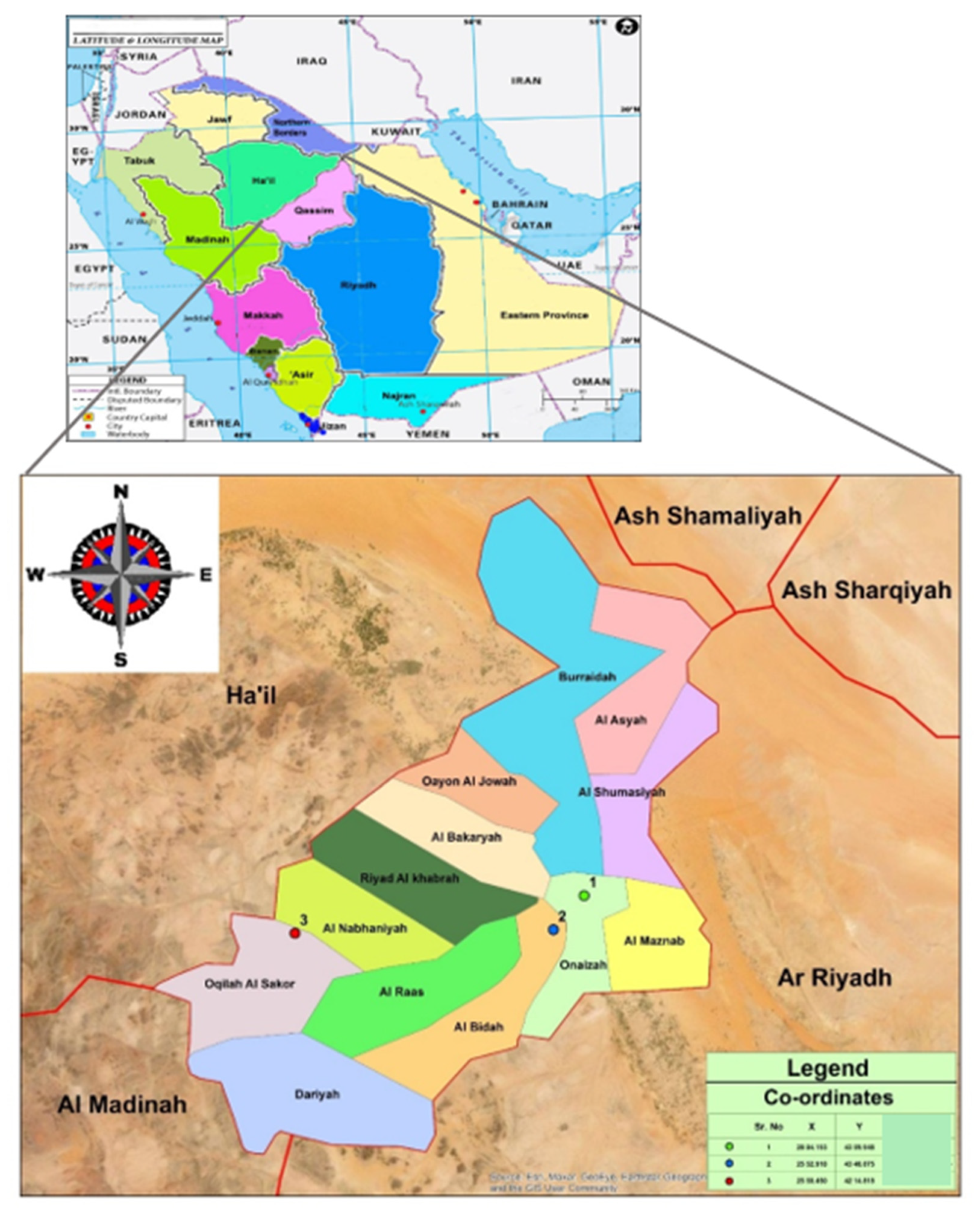
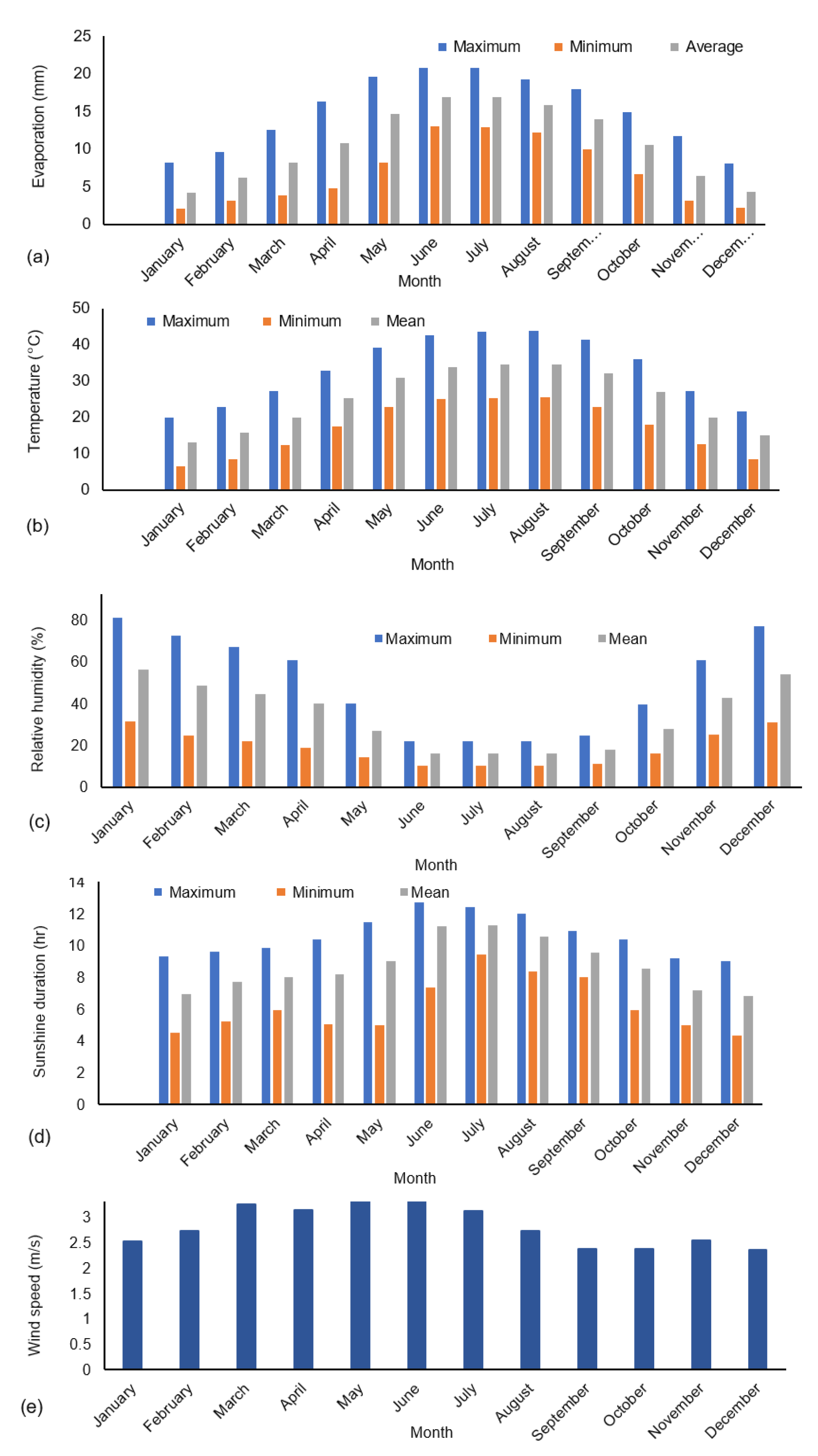
2. Study Area and Baseline Data

The present research began with the collection of a wide range of baseline data needed for i) calibrating and validating the Penman and Hamon equations and ii) training, validating, and testing soft computing models (ANN and ANFIS). The data for the mean daily values of the month, comprised of the temperature, sunshine hours, relative humidity, wind speed, and evaporation, were collected from the municipalities of Buraydah and Unayzah and Airport Authorities, Qassim, Saudi Arabia. The three stations use US-Bureau-Class-A evaporation-pan operated manually for the measurement of daily evaporation. It commonly has a diameter of 120.7 cm and height of 25.4 cm. It is fixed on a platform made of wood, which is installed on the ground. The location of the pan at all three stations has been selected very carefully to keep the pan away from trees and bushes and to allow the natural circulation of air around it. The daily evaporation was recorded as the depth of water (mm) lost from the pan. To estimate the actual pond or lake evaporation, a pan coefficient must be used to change the recorded pan-evaporation into pond/lake evaporation. The maximum and minimum type thermometers are being used to measure the temperature, i.e., a psychrometer for the relative humidity and anemometer to measure the wind speed at these stations. The other parameters were estimated on the basis of available monitored data (temperature, relative humidity, wind speed, and sunshine hours). The saturation vapor pressure, vapor pressure of free-flowing air, and net solar radiation were estimated on the basis of the diurnal course of temperature, relative humidity, and other meteorological constants/parameters (see equations 6 to 16 in the following text).

The study area is shown in Figure 1. Data from three weather stations were used in this research. Figure 1 shows the location of these stations, along with their coordinates. The stations record the pan-evaporation of three main locations of the Qassim Region. The same stations also have rain gauges for the measurement of rainfall. Rainfall in the Qassim Region usually occurs in winter. The three-day, two-day, and one-day maximum rainfall for this region is estimated to be 95, 92, and 86 mm, respectively. Figure 2a–d illustrates the past records of evaporation and the above-stated meteorological parameters. Figure 2a shows that the mean daily evaporation remains comparatively higher from May to September. Figure 2b shows that the temperature also reaches the maximum during these months. The relative humidity is comparatively lower during summer, while it is relatively higher during winter (Figure 2c). The sunshine duration is opposite to the relative humidity (Figure 2d). In Figure 2e, the wind speed also presents a similar pattern to the relative humidity. The average daily evaporation ranges from 4.2 mm/day in winter (December–January) to about 17 mm/day during summer (June–August). The maximum daily evaporation (40 years (1976 to 2016) mean for maximum evaporation) ranges from 8.2 mm/day during winter to 20.8 mm/day in summer.

The advection heat transfer from the hot earth surface to air masses is a common mechanism in warm-arid regions. This phenomenon has a significant impact on the pan-evaporation and should be taken into account carefully while developing pan-evaporation models for warm-arid regions. The whole area of Saudi Arabia is shown in Figure 1 to provide useful information related to the study area, monitoring data, and meteorological parameters of the study area.

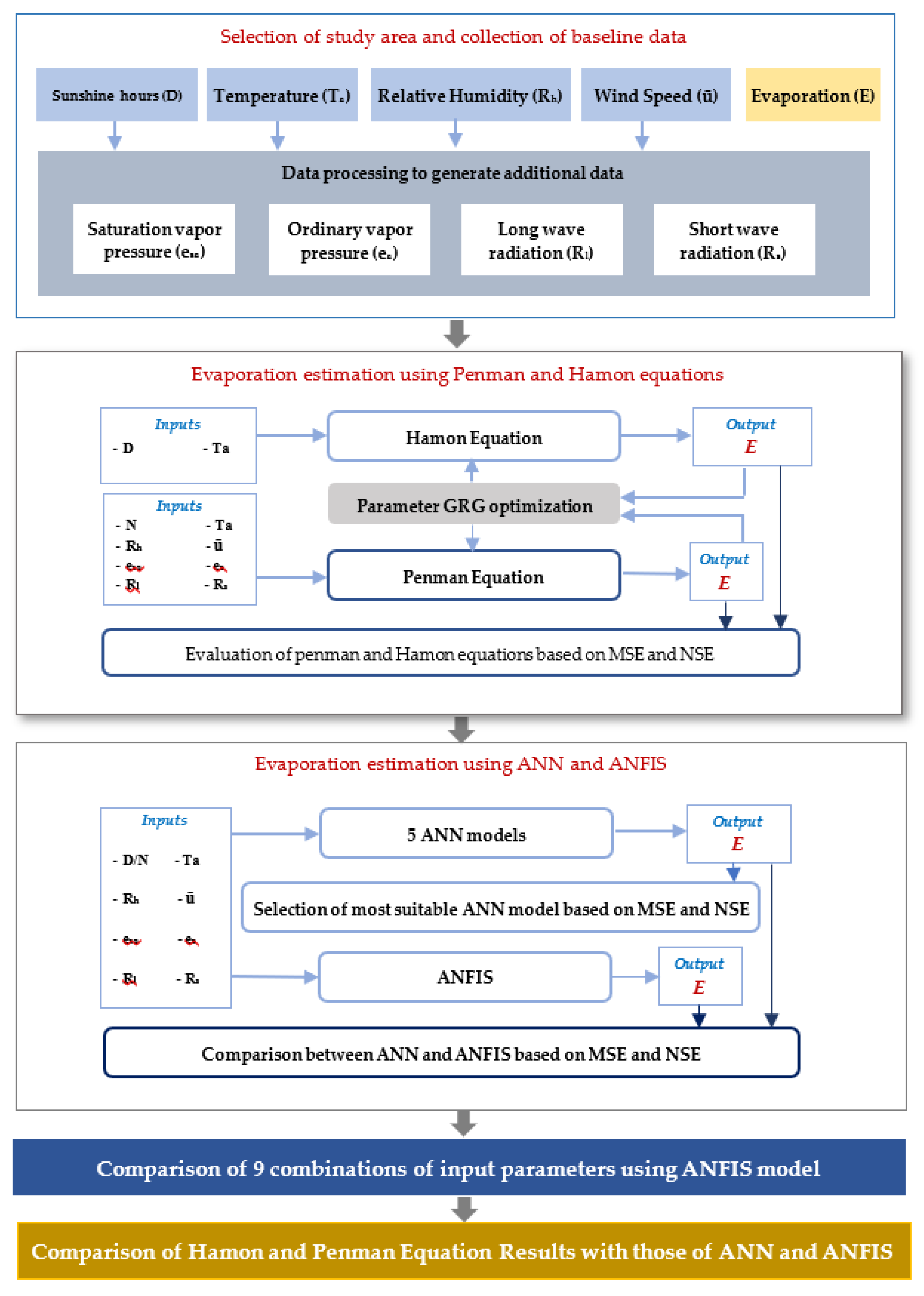
3. Materials and Methods

Figure 3 presents the methodological framework adopted in the present research. The data collection has been described in the previous section. The other steps involved in this context are described in the following sub-sections. The second task of this research was to develop models to estimate evaporation using various techniques, including ANN and ANFIS. New codes in MATLAB were written for the development of five ANN and ANFIS models for predictions of pan-evaporation. Penman and Hamon equations were also investigated and the General Reduced Gradient (GRG) optimization scheme was applied to identify the parameters of these equations for accurate estimations of pan-evaporation. GRG optimization was applied using Excel Solver.

3.1. Penman Equation

As stated in the introduction, there are many equations based on the laws of physics, empirical methods, and semi-empirical equations for the assessment of pan-evaporation [34]. The Penman Equation is considered to be the most robust and standard one because it encompasses most of the physics of the process of vaporization [4,17,35,36]. Both the energy-budget and the mass-transfer approaches are involved in the calculation of the amount of evaporation. This equation, however, requires exhaustive data, comprising sunshine hours, wind speed, temperature, and relative humidity, etc. In the case of data scarcity, the optimization of its parameters is a highly challenging task.

The method defines the daily evaporation as [34,35,36,37,38]

$$E=\frac{\Delta }{\Delta +\gamma }\frac{R_{net}}{\lambda }+\frac{\gamma }{\Delta +\gamma }\frac{A_1}{\lambda }\left(1+A_2\overline{u}\right)\left(e_{sa}-e_a\right),$$

(1)

where $R_{net}$ expresses the net solar-radiation in Million Joules/m²/day (MJ/m²/day), λ is equal to the latent heat of vaporization in MJ/kg, $\overline{u}$ is the mean daily wind speed in m/s, $e_{sa}$ is the mean daily saturated vapor pressure in Pa, $e_a$ is the mean daily vapor pressure of free-flowing air in Pa, $\gamma$ is the psychrometric constant (kPa °C⁻¹), and Δ is the average slope of the temperature curve and saturated vapor pressure [34,35,36,39,40].

It is worth mentioning here that the conversion of solar radiation absorbed for evaporation into its equivalent evaporated water (mm/day) is very important in Penman’s Equation. In some references [41], the first term of Penman’s Equation is written as $A\prime \Delta /\left(\Delta +\gamma \right),$ where $A\prime$ is the measured or estimated energy available from the free water surface expressed in mm/day. R_net/λ gives the same water equivalent in Equation (1) and (3). The term $\Delta$ can be expressed by the equation given below in terms of the mean air temperature T_mean. $A_1$ (coefficient before the adventive part of Equation (1)) and $A_2$ (the wind speed factor) are the two constants with values of 6.43 and 0.54 in the original equation, respectively [41].

$$\Delta =\frac{2503 \exp \left(\frac{17.27 \times T_{mean}}{237.3 + T_{mean}}\right)}{{\left(237.3+T_{mean}\right)}^2},$$

(2)

$$R_{net}=\left(1-\alpha \right)R_s+R_l,$$

(3)

where $R_s$ is equal to the shortwave incoming solar radiation (J m⁻² day⁻¹), α is the albedo coefficient, and $R_l$ is equal to the longwave solar radiation [34,36,42,43]. The albedo constant is a very important parameter in Penman’s Equation. Its value should either be measured or can be taken from tables and guidelines provided in past works for the study area. The albedo values used in this study were taken from guidelines provided by reference [44]. These are average values over the year for stations located in the oasis and the desert.

$$R_s=\left(as+\left(\frac{bs\times n}{N}\right)\right)\times \left(\frac{1440}{\pi }\right)\times G_{sc}\times dr\times \left(\omega s\times \sin (Ø)\times \sin (\delta )+\cos (Ø)\times \cos (\delta )\times \sin \left(\omega s\right)\right)$$

(4)

where n is the actual sunshine duration (hour), N denotes the maximum possible sunshine duration or daylight hours (hour), as is the regression constant, as + b_s designates the extraterrestrial radiation fraction reaching the earth during clear days (for n = N), $G_{sc}$ is the solar constant (0.0820 MJ m⁻² min⁻¹), and $d_r$ is the inverse relative distance (Earth–Sun).

$$d_r=1+0.033\times \cos \left(\frac{2\pi J}{365}\right),$$

(5)

where J represents the number of days in a year, i.e., from 1 January to 31 December (365 or 366 in a leap year).

$$\delta =0.409\times \sin \left(\frac{2\times \pi \times J}{365}-1.39\right),$$

(6)

where $\delta$ is the solar declination.

$${\omega }_s=ArcCos\left[-TAN(Ø)\times TAN\left(\delta \right)\right],$$

(7)

where ${\omega }_s$ is the sunset hour angle and $Ø$ is the latitude expressed in radians.

$$R_l=\sigma \times \left(\frac{{(Tmax+273.16)}^4+{\left(Tmin+273.17\right)}^4}{2}\right)\times \left(0.34-0.14\times SQRT\left(ea\right)\right)\times \left(1.35\times \frac{R_s}{R_{so}}-0.35\right),$$

(8)

where R_so represents the clear sky solar radiations; $R_l$ denotes the net outgoing longwave radiation (MJ m⁻² day⁻¹); and $\sigma$ is the Stefan–Boltzmann constant (4.903 × 10⁻⁹ MJ K⁻⁴ m⁻² day⁻¹) [41].

$$e_a=\frac{\left(e_{\left(T_{\max }\right)}\times \frac{R_h{}_{\left(min\right)}}{100}+e_{\left(T_{\min }\right)}\times \frac{R_h{}_{\left(max\right)}}{100}\right)}{2},$$

(9)

$$e_{\left(T_{\max }\right)}=0.6108\times \exp \left(\frac{\left(17\cdot 27\times T_{\max }\right)}{T_{\max }+237.3}\right),$$

(10)

$$e_{\left(T_{\min }\right)}=0.6108\times \exp \left(\frac{\left(17\cdot 27\times T_{\min }\right)}{T_{\min }+237.3}\right),$$

(11)

$$e_{sa}=e_{\left(T_{\mathrm{mean}}\right)}=0.6108\times \exp \left(\frac{\left(17\cdot 27\times T_{\mathrm{mean}}\right)}{T_{\mathrm{mean}}+237.3}\right),$$

(12)

$$T_{\mathrm{mean}}=\frac{T_{\max }+T_{\min }}{2},$$

(13)

where, $T_{\mathrm{mean}}$ is the mean daily air temperature (°C), $T_{\max }$ is the maximum daily air temperature (°C), and $T_{\min }$ is the minimum daily air temperature (°).

3.2. The Hamon Equation

The Hamon-derived evaporation equation is as simple as possible. He only used two main input parameters, including the temperature and sunshine hours [45,46]. The developed equation is applicable for both humid and dry climatic conditions. According to this method, the evaporation may be calculated as follows [45,46]:

$$E=B_1{\left(D\right)}^{B_2}{10}^{\left(\frac{B_3 T_{mean}}{T_{mean}+273}\right)},$$

(14)

where D is the maximum sunshine duration ratio and T_mean is the mean air temperature. The value of D may be estimated using the equation given below. $B_1$, $B_2$, and $B_3$ are constants with typical values of 0.63, 2.0, and 7.5, respectively.

$$D=\frac{1}{90}\arccos \left(-\tan (Ø).\tan 23.45°\sin \left(\frac{J-80}{365}\right)360°\right)$$

(15)

In this equation, “ϕ “ is the latitude and J represents the Julian day.

3.3. Identification of Parameters of Penman and Hamon Equations Using Optimization

Although the Penman Equation is mainly based on the laws of physics, its application usually produces a very high accuracy and depends on the place. Similarly, Hamon’s Equation is also data-dependent. Therefore, the optimization of some parameters is required, as mentioned in the “Introduction” section. Parameters of the Penman and Hamon equations were identified using the General Reduced Gradient (GRG) Optimization Technique [47]. The values of constants $A_1$ and $A_2$ in Equation (1) and the value of $\alpha$ in Equation (3) were identified through parameter optimization of the Penman Equation. Similarly, the constants $B_1$, $B_2$, and $B_3$ in Equation (14) were chosen for the optimization of parameters of Hamon’s Equation. Two options of parameter optimization were investigated. In option 1, the values of $A_1$ and $\alpha$ were chosen, and the values of $A_1$ and $A_2$ were selected for the case of the Penman Equation in option 2. In the case of Hamon’s Equation, the constants $B_1$, $B_2$, and $B_3$ were taken as parameters for optimization in the first option and only the two parameters $B_1$ and $B_3$ were adopted in the second option. Two parameters were chosen to conduct a fair comparison of the results of the Penman and Hamon equations. The values were no longer taken as constants; rather, these parameters were changed during the process of optimization to minimize the objective function in the case of error (MSE) and to maximize the objective function in the case of NSE using the General Reduced Gradient (GRG). The first half of measured evaporation data was used for optimization/calibration. Finally, the GRG optimization generated the globally best possible values of these parameters. The results of Penman and Hamon equations obtained with these new values of parameters were compared with the remaining half of recorded data for validation of the equations.

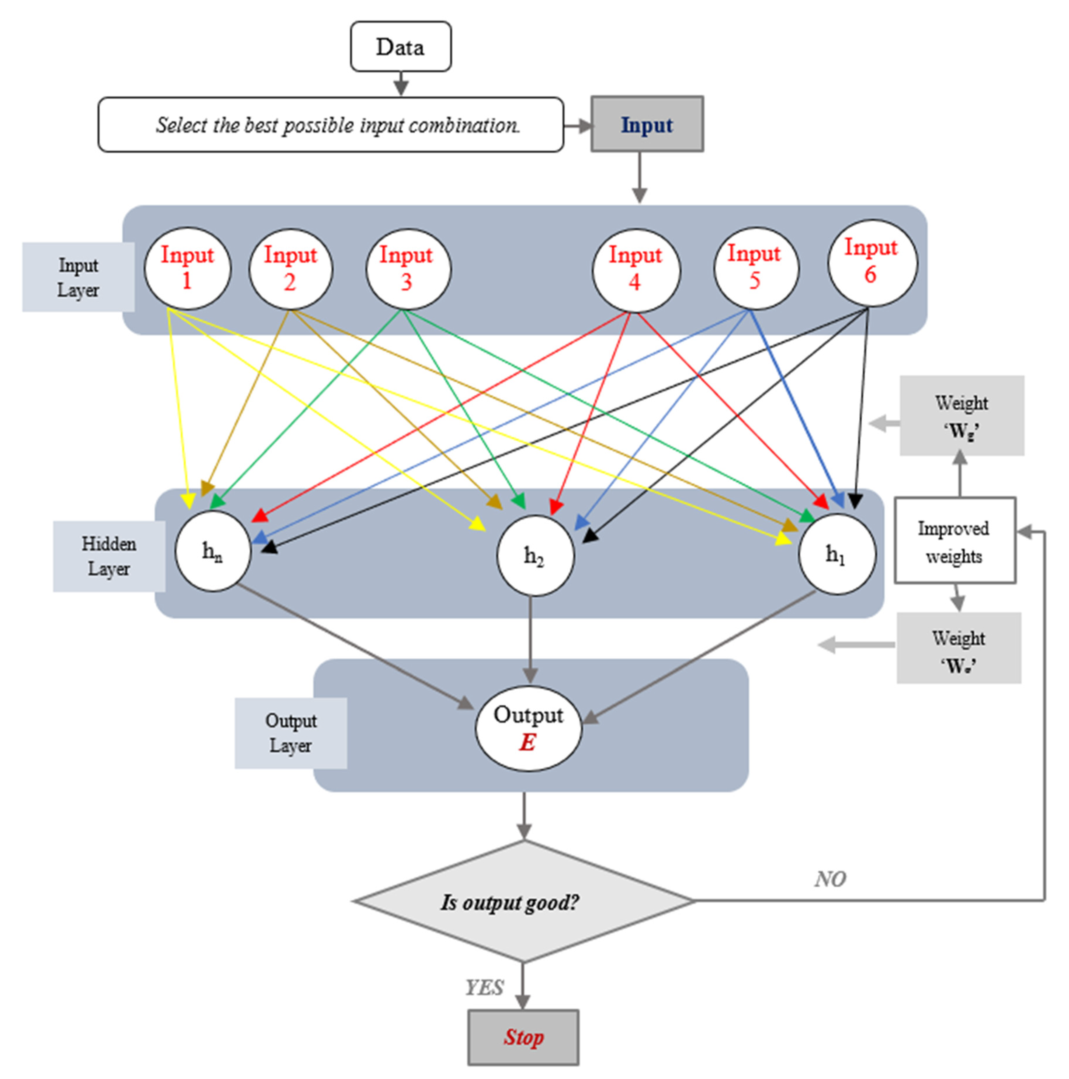
3.4. Artificil Neural Networks

Being a computational model, in an Artificial Neural Network (ANN) model, encouraged by the networks of biological neurons, the neurons calculate output values from inputs. It learns from its previous experience and errors in a non-linear parallel processing manner. The neuron is the basic determining entity that computes based on a number of inputs and provides one output compared with a target value. The internal structural arrangement performs the computation process in which hidden layers employ the backpropagation (BP) and the feed-forward mechanism to generate outputs with the desired accuracy. The learning is based on reinforcement (supervised) and unsupervised (no target) type learning. Overall, there are three stages of the model, called training, validation, and testing. The provided data are divided into three parts accordingly, for example, 60% for training, 20% for validation, and 20% for testing; 70% for training, 15% for validation, and 15% for testing; or any other combination. Training is a highly important feature of ANN. It is a common practice to use randomly divided data for the training, validation, and testing of ANN models. However, in the case of parameter optimization of evaporation equations, the employment of organized data (50% for calibration and 50% for validation) is the most common approach. Therefore, both the cases were tested for ANN to observe the impact of data division on the random basis or organized manner. For a fair comparison of model results, all of the work related to comparisons of various models was conducted using organized data.

There are several types of training functions. We assessed the performance of the five models M1, M2, M3, M4, and M5 with five different training functions, as described in

Table 1. Various training functions used for ANN models.

Model	Function	Description of Training Function	Model	Function	Description of Training Function
M1	trainlm	Levenberg–Marquardt BP	M4	trainrp	Resilient backpropagation (Rprop)
M2	trainbr	Bayesian regularization	M5	trainscg	Scaled conjugate gradient BP
M3	trainbfg	BFGS Quasi-Newton BP	-	-	-

. The other important features of an ANN can be described as follows:

• The network architecture has an input layer and output layer. In the case of multiple hidden layers, it is also known as the Multi-Layer Perceptron (MPL);
• The hidden layer operates like a “distillation layer” that distills several key patterns from the inputs and forwards them onto the next layer. It enhances the efficiency and speed of the network by identifying the primary information from the inputs and ignores the redundant information. In this research, models with double and triple hidden layers, represented by double layer (DL) and triple layer (TL), were tested. Different numbers of neurons can be chosen in hidden layers. Sheela and Deepa [48] reviewed various methods for selecting the hidden neurons. Some researchers have used a hit and trial approach for selecting the optimal number of neurons in hidden layers; either starting from a lower number (undersized number of hidden neurons) and increasing the number of neurons in every trial to reach an optimal number by reducing the error to the minimum possible or vice versa. The same number of neurons in each type of hidden layer (DL or TL) ANN model or decreasing the number of neurons from a lower to higher hidden layer model have been recommended by many researchers [48,49,50,51]. We investigated an architecture with 5, 10, and 15 neurons in hidden layers in both the cases of DL and TL;
• Two significant purposes of the activation function are that i) it captures the non-linear relationship between the inputs, one by one, and the output, and ii) it helps convert the input into a more useful output.

A reliable model predicts the results close to the actual (observed) values with a high accuracy. In modern ANN, it is obtained by a combination of optimization approaches where certain parameters called weights (W) are adjusted to find the best possible outputs. The key to obtaining a reliable model is to find the “optimal values of W” that minimize the prediction error. A general flowchart of ANN is given in Figure 4. The output accuracy may significantly be impacted by the combination of input variables. This research studied the impact of eight input combinations, as given in Figure 5.

Figure 4. Modeling approach representing the multilayer perceptron (a feed-forward-Artificial Neural Network (ANN)) with six input parameters (after Almuhaylan, et al. [52]).

Figure 4. Modeling approach representing the multilayer perceptron (a feed-forward-Artificial Neural Network (ANN)) with six input parameters (after Almuhaylan, et al. [52]).

One of the combinations is further elaborated below. The equation given below represents the case of only two input variables (say temperature and wind speed (input combination C2)):

$$E_i=f(W_{\left(1i\right)}\times T_i+W_{\left(1i\right)}\times U_i+C),$$

(16)

where f stands for ‘a function of’; T_i, U_i (ith value of inputs, i.e., temperature T and wind speed U), W_(1i), and W_(2i) are the i-th weights of the inputs, respectively; and C is the constant for the node with output Ei, representing the evaporation. The ANN calculates the outputs (evaporation) on the basis of a function mentioned above and all the information about inputs at all the nodes. The predicted output (estimated evaporation) is compared with the actual output (measured evaporation). If the output does not match the required output, the backpropagation process is performed, which re-adjusts the weights to match the output to the true value (the target evaporation). In other words, the backpropagation process involves an optimization problem, as described above, for the weights to reduce the error between the measured and predicted evaporation.

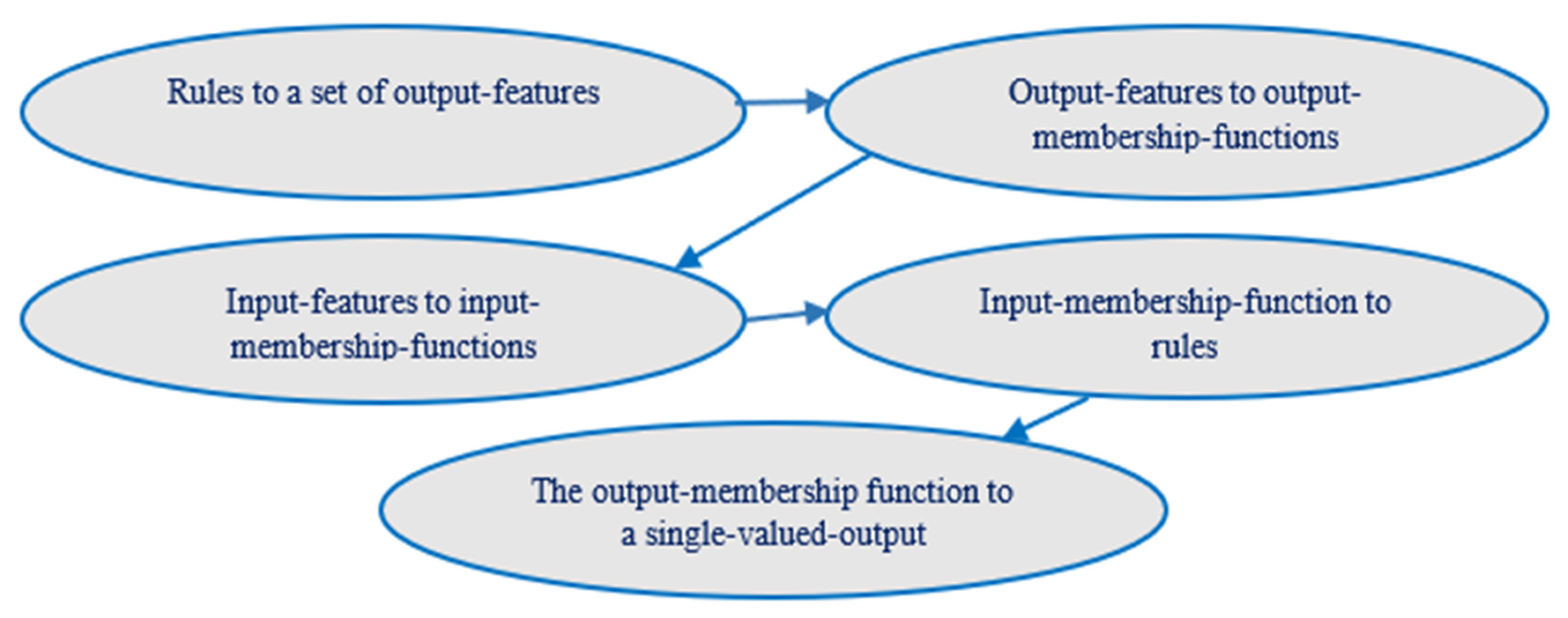
3.5. Adaptive Neuro-Fuzzy Inference Systems

Adaptive Neuro-Fuzzy Inference Systems are hybrid artificial intelligence models and an optimization algorithm is the prevailing modeling approach. ANFIS consists of an adaptive ANN and a fuzzy inference system. It uses a hybrid-learning rule merging gradient descent, backpropagation, and a least-squares algorithm to estimate a set of parameters. A receptive mathematical structure of ANFIS can estimate a large class of complex nonlinear systems with the desired precision. Figure 6 shows the following five layered structure of ANFIS, which can be presented as follows:

Layer 1: Fuzzy layer in which every node is an adaptive node. Membership functions such as the generalized bell membership function and Gaussian membership function are used as node functions;

Layer 2: Product layer in which each node output shows the firing strength of a rule;

Layer 3: Normalized layer in which every node represents the normalized firing strength of each rule;

Layer 4: De-fuzzy layer in which every node is an adaptive node with a node function indicating the contribution of the rules to the overall output. Parameters in this layer will be referred to as consequent parameters;

Layer 5: Total output layer which presents the de-fuzzified (single) valued output.

3.6. Performance Evaluation of Evaporation Models

The performance of the models was assessed by the Nash–Sutcliffe efficiency (NSE), as given below [53]:

$$NSE=\left(1-\frac{{{\displaystyle \sum }}_{i=1}^n{\left(E_{mi}-E_{pi}\right)}^2}{{{\displaystyle \sum }}_{i=1}^n{\left(E_{mi}-{\overline{E}}_{mi}\right)}^2}\right),$$

(17)

where E_mi is the value of the measured evaporation for the ith data point, E_pi is the predicted value of evaporation for the same data point, ${\overline{E}}_{mi}$ is the mean value of E_m, and n is the total number of data points used to test the models. The performance ranges of models are defined in

Table 2. Performance levels for the evaluation of evaporation models.

NSE Range	Performance Level
0.75 to 1.00	Very Good
0.65 to 0.75	Good
0.50 to 0.65	Satisfactory
0.4 to 0.50	Acceptable
≤0.4	Unsatisfactory

[54,55].

The mean square error (MSE) is the other performance measure of the developed evaporation equations:

$$MSE=\frac{{{\displaystyle \sum }}_{i=1}^n{\left(E_{mi}-E_{pi}\right)}^2}{n}.$$

(18)

The number of epochs and the computer time consumed by ANN models are intentionally not included in the “Results and Discussion” section because they are not so significant for a practical engineer working in the field of hydrology.

4. Results

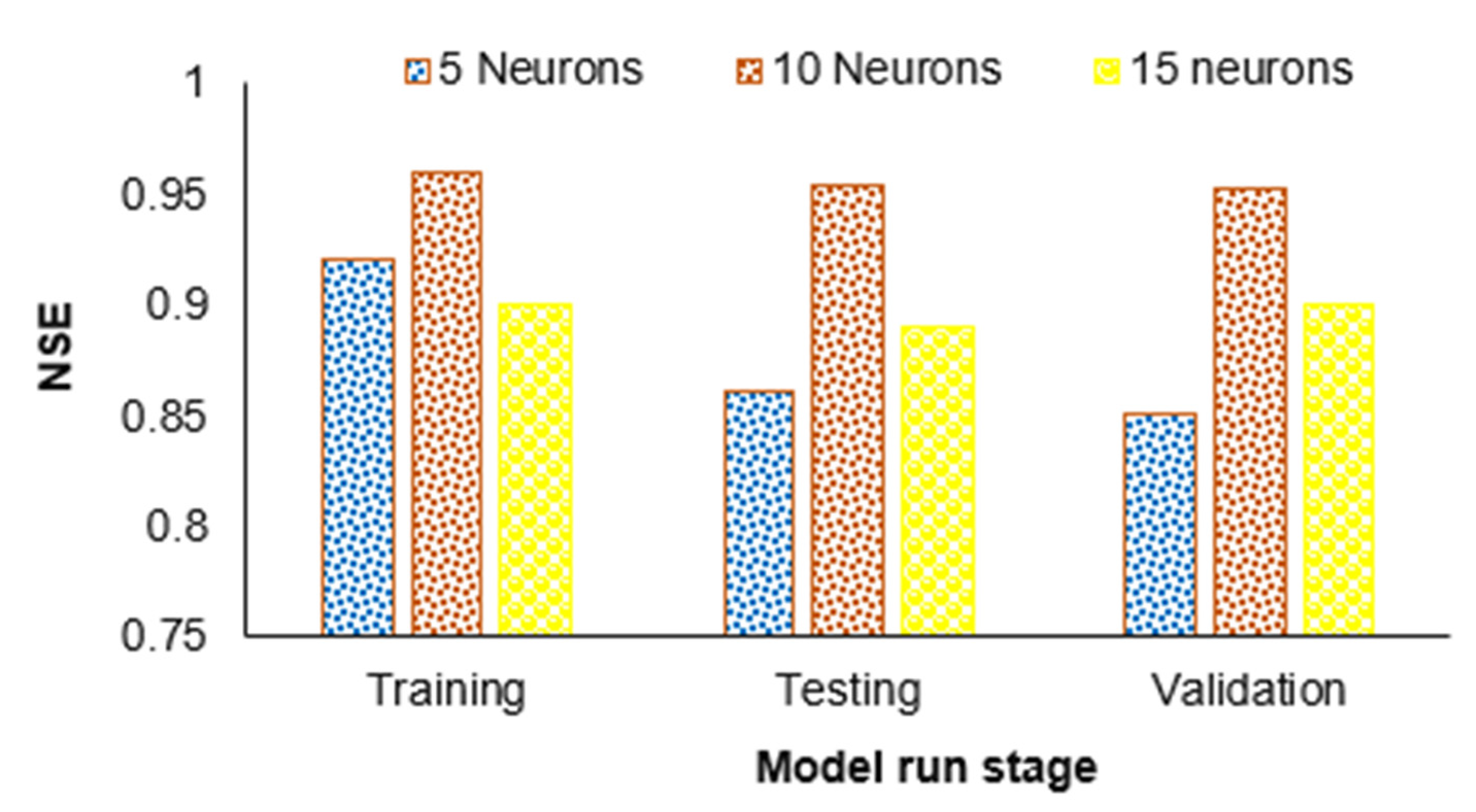
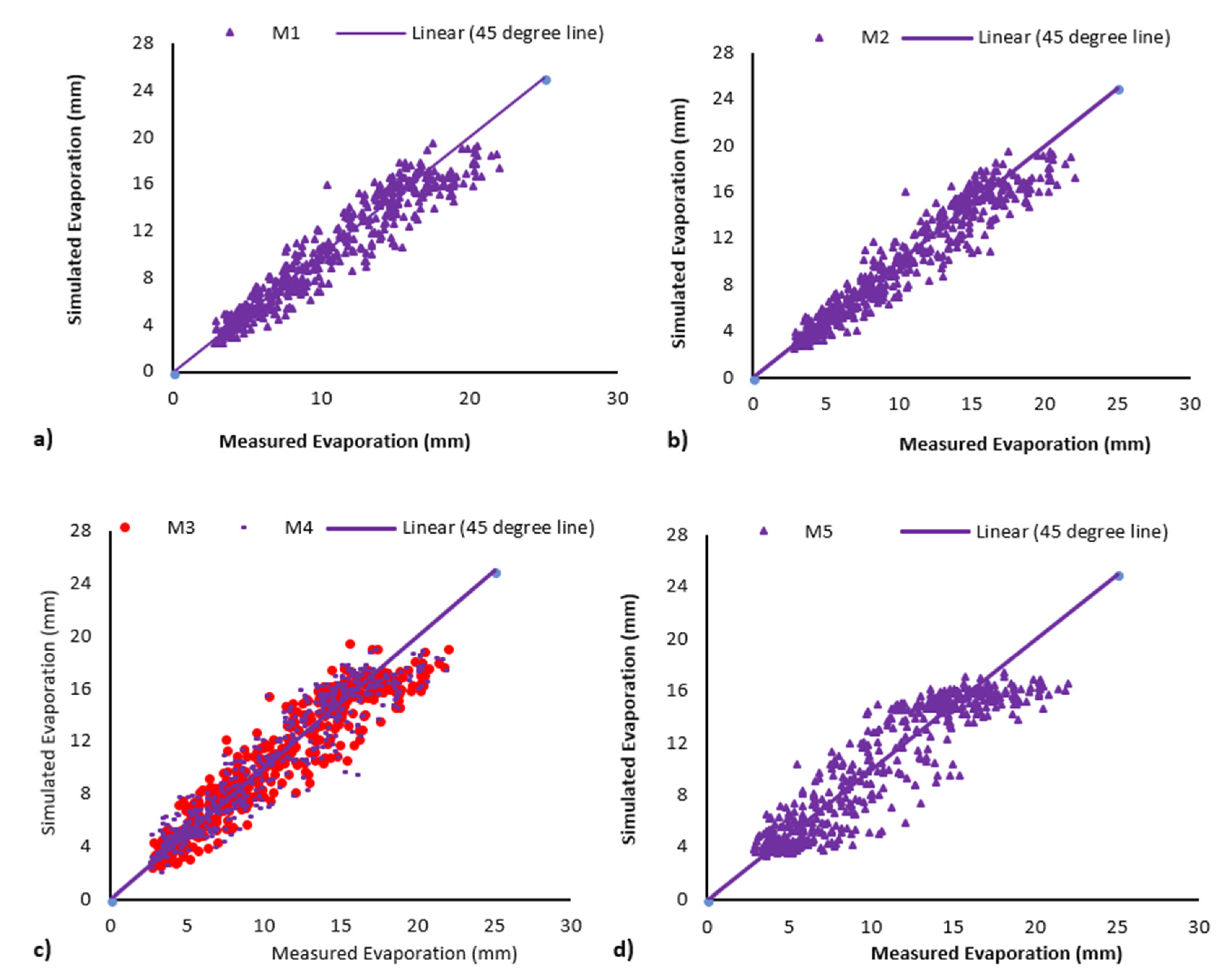
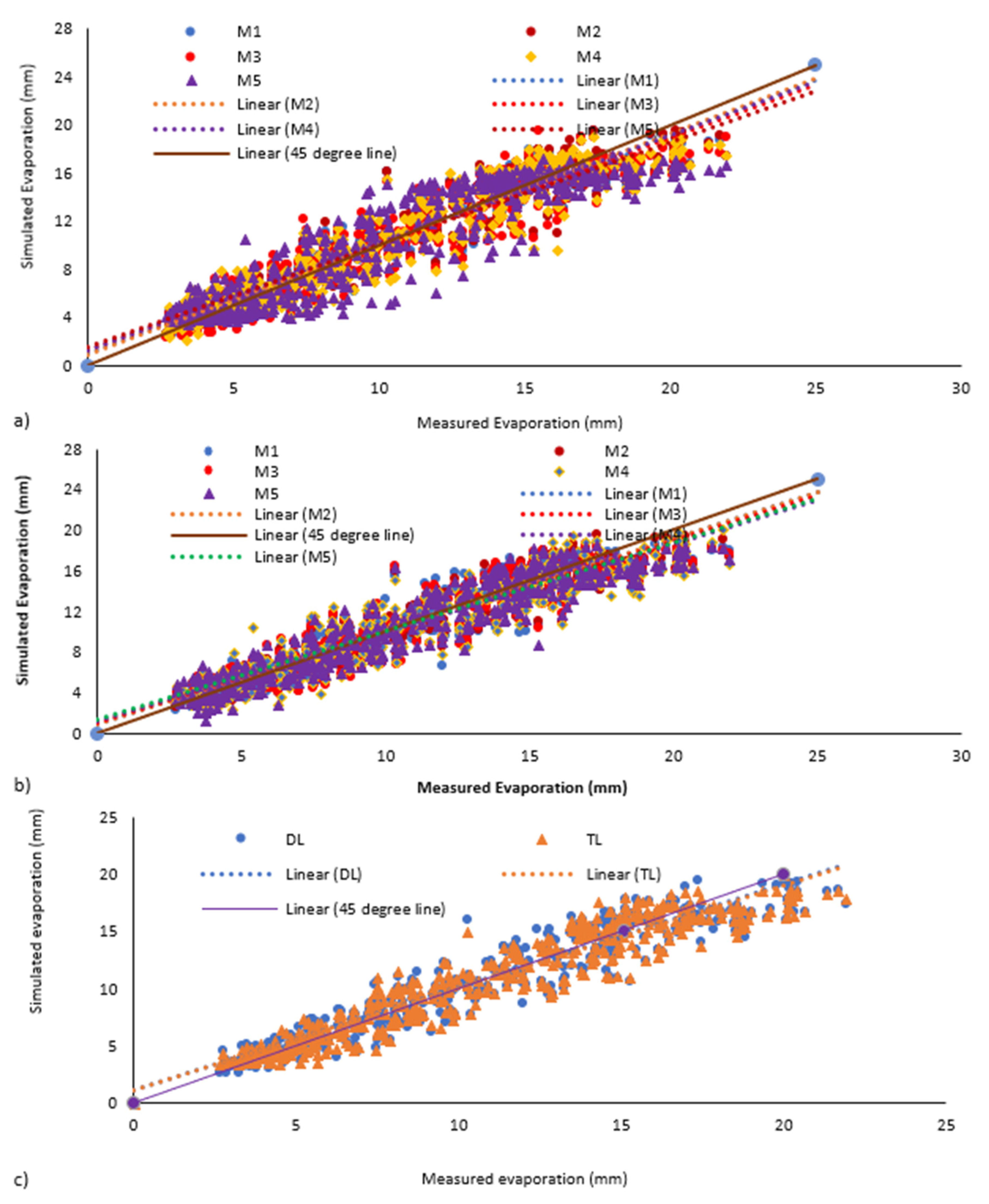
4.1. Comparison of Results of ANN Models with Various Architectures

Figure 7 shows the impact of various architectures of DL-ANN models. It can be observed that the architecture with 10 neurons in hidden layers produces better results than that of 5 and 15 neurons in all cases of training, testing, and validation. NSE values up to 0.96 were achieved. Similar results have been reported by Jimenez et al. [56] and Almuhaylan et al. [52]. However, it is worth mentioning that in the case of 5 and 15 neurons, the results are also promising. The NSE value in not less than 0.85 in any case, which indicates the high performance of models (NSE values ranging from 0.75 to 1 represent a “very good” performance [54,55]). However, the use of a complicated architecture with a higher number of neurons is not preferable, because it consumes more computer time, without any additional benefit. Therefore, the further analysis included in this research was conducted using an ANN architecture with 10 hidden neurons.

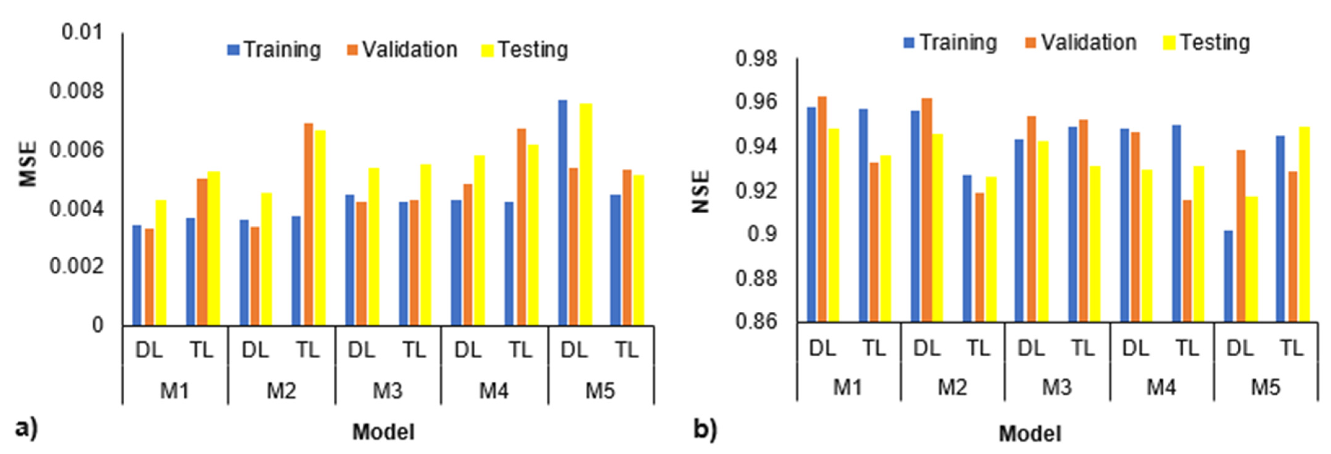
4.2. Comparison of DL- and TL-ANN Models with Five Different Training Functions

A comparison of the five double and triple layer ANN models (M1–M5) with 10 hidden neurons for the simulation of pan-evaporation is presented in Figure 8a,b, Figure 9a–d, and Figure 10a–c. It can be observed that both types of model perform equally well. The maximum value of NSE is 0.963 and the minimum is 0.902. The MSE values lie in the range of 0.0077 to 0.0033 (Figure 8a,b).

The performance of double layer ANN models (M1–M5) in comparison with the line is shown separately in Figure 9a–d. The predicted verses measured evaporation values lie close to the 45° line, indicating the good performance of the models. There is no insignificant scattering of predicted evaporation from the 45° line (1:1 line).

The performance of five DL- and TL-ANN models is shown by another indicator in Figure 10a–c. In these figures, the trend lines of each model are shown in comparison to the 45° line. All trend lines are found close to the 45° line. All the models exhibit a similar trend and high performance. In this context, our results are in line with the results of Bruton et al. [22] and Alsumaiei [20]. According to both of these studies, there is no substantial improvement in the performance of ANN in response to changing the number of hidden layers. However, the double layer models can be placed on merit no 1 compared to the triple layer models on the basis of having slightly higher values of NSE and lower values of MSE compared to triple layer ANN models. Additionally, the triple layer models are relatively complicated and consume more computer time, without gaining any additional accuracy.

Looking at various parts of Figure 8, Figure 9 and Figure 10, it can be observed that, although there is a very small difference in the statistical parameters of various models, (

Table 3. Values of statistical indicators for five DL and TL models (M1–M5) (with 10 hidden neurons).

Model Name	Layers	MSE			NSE
		Training	Validation	Testing	Training	Validation	Testing
M1	DL	0.003406	0.003286	0.004264	0.958	0.963	0.948
	TL	0.003671	0.005014	0.005245	0.957	0.933	0.936
M2	DL	0.003586	0.003386	0.004496	0.9565	0.9622	0.9458
	TL	0.003746	0.006913	0.006671	0.927	0.919	0.926
M3	DL	0.004448	0.004203	0.005338	0.94361	0.95388	0.9421
	TL	0.0042	0.00426	0.005485	0.949	0.952	0.931
M4	DL	0.004272	0.004836	0.005763	0.9479	0.9469	0.9295
	TL	0.00422	0.006738	0.006176	0.95	0.916	0.931
M5	DL	0.007715	0.005368	0.007548	0.9018	0.93888	0.91695
	TL	0.004495	0.005339	0.005095	0.945	0.929	0.949

), model 1 with Levenberg–Marquardt Backpropagation as the training function is the top merit model, with the highest values of the performance indicators.

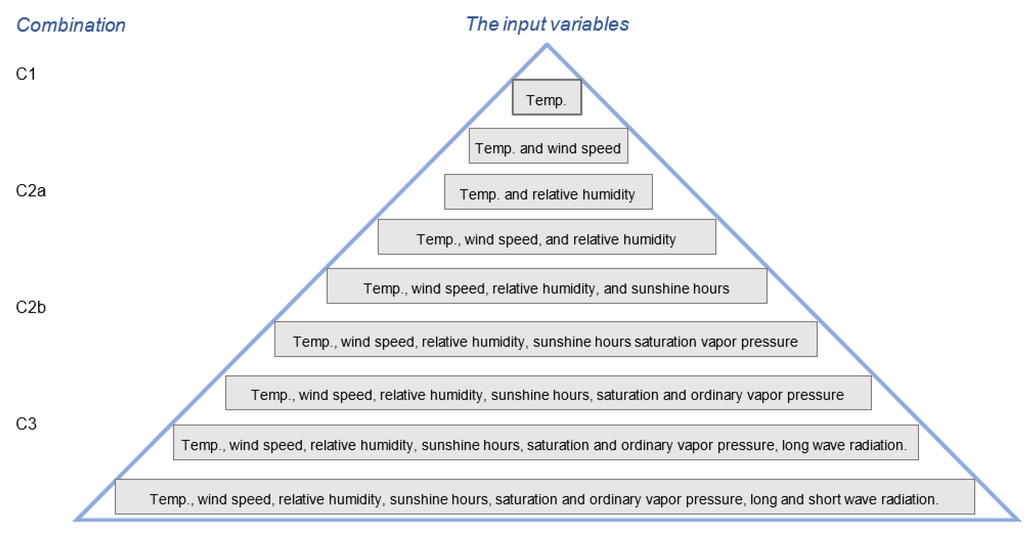
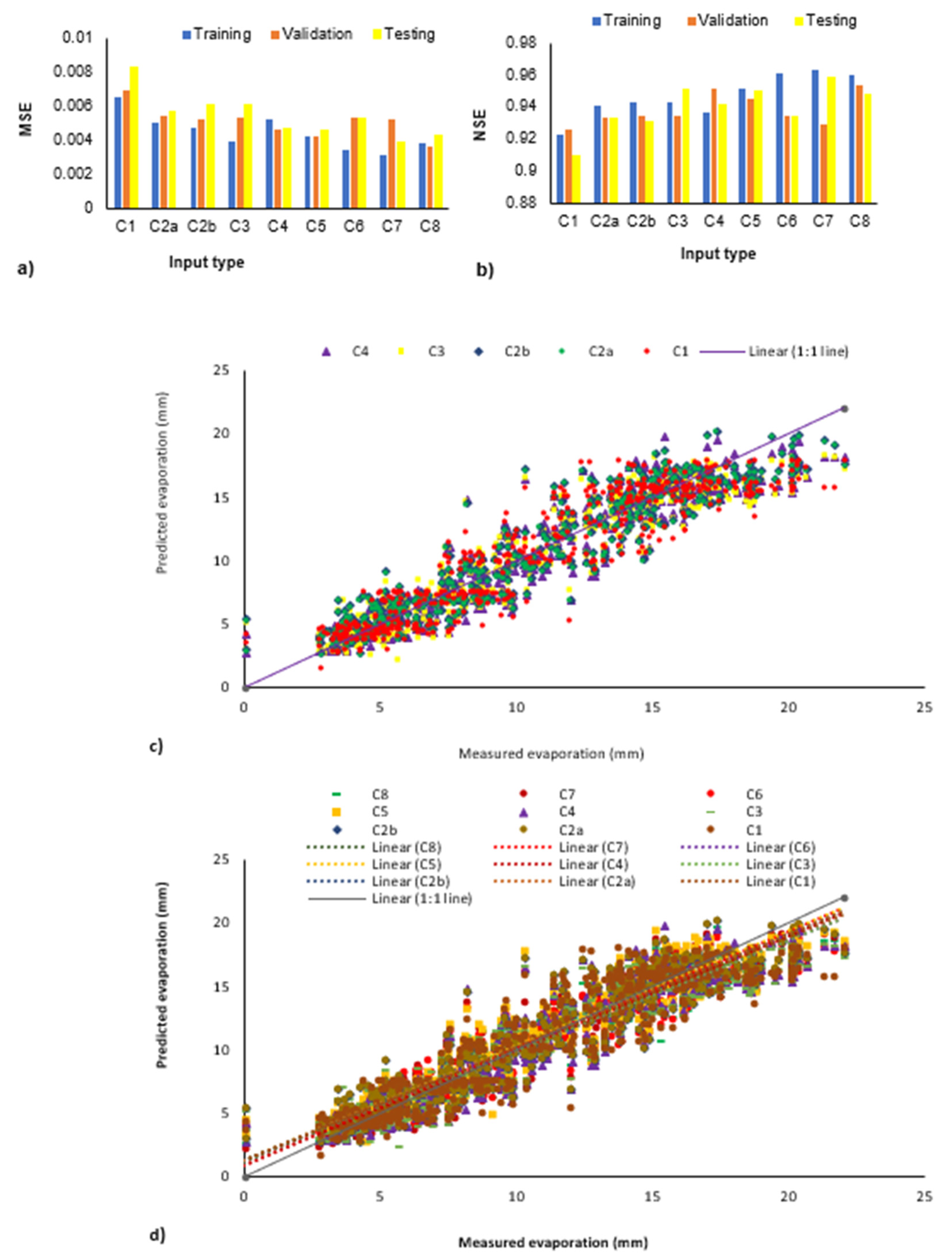
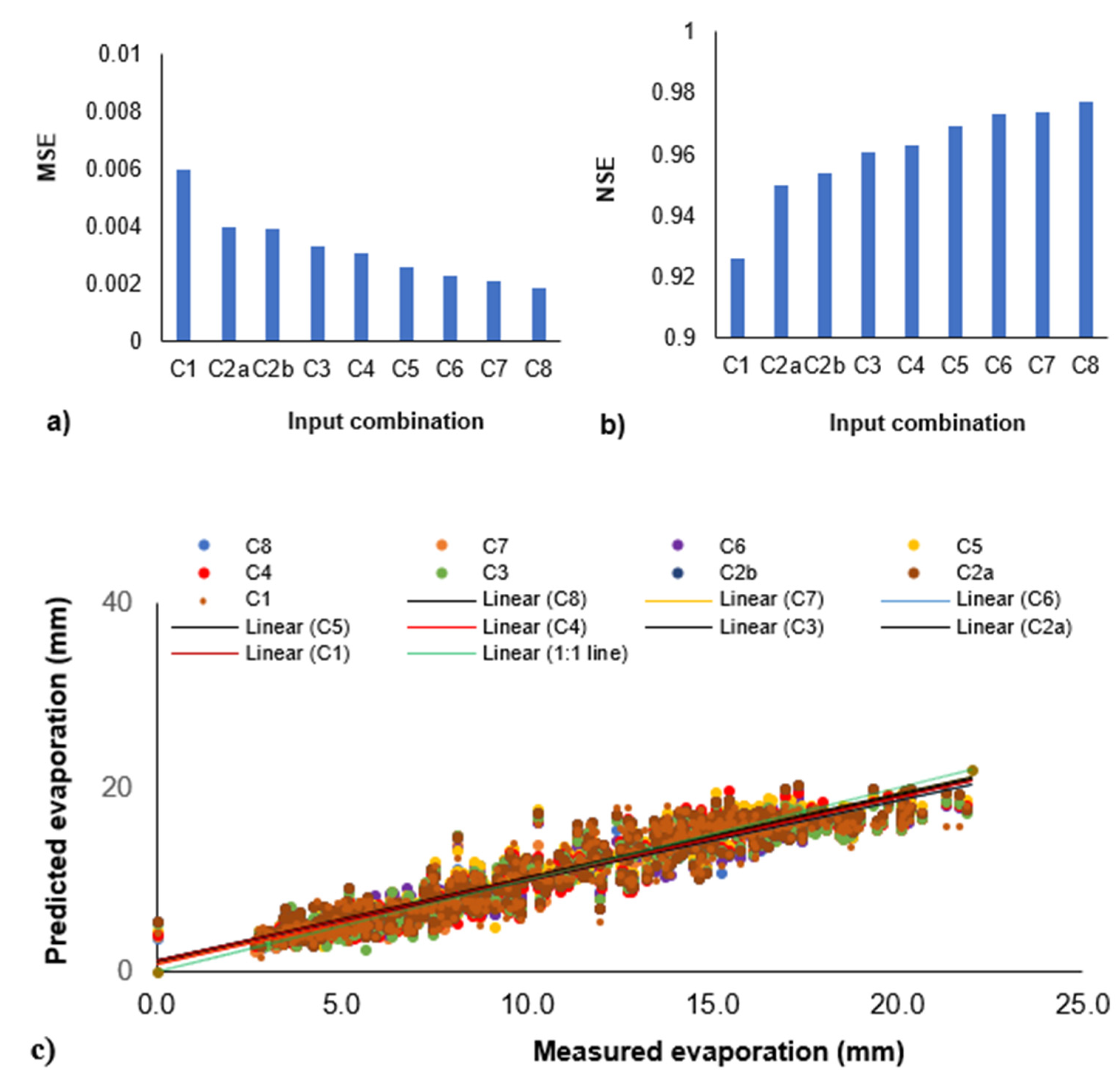
4.3. Impact of the Number of Input Parameters

Figure 11a–c shows the performance of the ANN model M1 with 10 hidden neurons for eight various combinations of input variables. Figure 11a,b shows the statistical indicators MSE and NSE for the training, validation, and testing stages of models. It can be observed that all of the input combinations produce acceptable results for the prediction of pan-evaporation using ANN models. The MSE lies in the range of 003 to 0.008, and NSE is in the range of 0.91 to 0.96 (

Table 4. Range of statistical indicators (MSE and NSE) for various input combinations for the ANN-DL-M1 model.

	MSE			NSE
	Training	Validation	Testing	Training	Validation	Testing
Maximum	0.0065	0.007	0.008	0.96	0.95	0.96
Minimum	0.003	0.0036	0.004	0.92	0.92	0.91

). Figure 11c shows an insignificant scatter of predicted values from the 45° line for all the eight input combinations. Combination C1 has only one input variable; the mean daily temperature shows quite acceptable results of predicted evaporation with MSE values of 0.0065, 0.0069, and 0.0083 and NSE values of 0.923, 0.926, and 0.91 in the training, validation, and testing stages respectively. The scatter around the 45° line in Figure 11c is also not significant. The evaporation process is mainly dependent on the temperature. Therefore, these results are very logical and represent a real physical phenomenon. The combination C1 can be considered the simplest case and highly suitable for countries having a scarcity of data.

The combinations C2a and C2b each include two variables as the input. The combination C2a involves the wind speed, with the mean temperature as an input variable, and C2b has the relative humidity with the mean temperature as an input variable. It comparatively enhanced the performance of ANN in simulating the pan-evaporation, which is visibly reflected by the statistical indicators. The combination 2a has MSE values of 0.00498, 0.0055, and 0.0056 and NSE values of 0.94, 0.934, and 0.933 in the training, validation, and testing stages, respectively. Similarly, the combination C2b has MSE values of 0.00469, 0.0052, and 0.006 and NSE values of 0.943, 0.935, and 0.931 in the training, validation, and testing stages, respectively. The enhancement in the performance of ANN due to the addition of the wind speed or relative humidity is quite logical because of the fact that it reflects the role of the wind speed and relative humidity in the process of evaporation. As the process of evaporation is a diffusive one, a vapor pressure gradient is essential for the occurrence of evaporation. Both of these variables of the wind speed and relative humidity assist in the process of evaporation and help remove water vapor from the surface of water bodies by upholding the vertical vapor pressure gradient between the overlying-air and the water body surface. Combination 3 includes three important meteorological input variables, consisting of the mean temperature, wind speed, and relative humidity, as input parameters. It predicted pan-evaporation approximately as effectively as models C2a and C2b. This is reflected by the MSE values of 0.00395, 0.005, and 0.006 and NSE values 0.943, 0.935, and 0.951 in the training, validation, and testing stages, respectively.

The combinations C4, C5, C6, C7, and C8 contain four, five, six, seven, and eight variables, respectively, as input parameters. The excessive meteorological inputs resulted in a relatively higher model efficiency (see Figure 11a–c). It is worth mentioning that in these combinations (C4 to C8), some variables were estimated as functions of temperature and wind speed. Due to missing information for additional variables (given in Figure 5 for C4 to C8) in the study area, the basic variables were used more than once in different ways. For example, in combination 3, the saturation vapor pressure was used as an input variable, which was calculated by the temperature, i.e., also an input variable in the model. Similar examples are also noticeable in other combinations. However, the real-time data for these additional variables (e.g., saturation and ordinary vapor pressure and radiation) available in developed countries should be used for simulations of C4 to C8.

Theoretically, a Machine Learning model should be able to detect the complex relationships between independent and dependent variables from the input data at the calibration stage. This ability is improving by optimizing the model’s architecture. Therefore, higher numbers of parameters are not always recommended due to the relatively higher complexity of models and scarcity of recorded data. The gain in efficiency is not significant compared to the difficulties faced in collecting exhaustive data in developing countries. Furthermore, researchers have considered it as overfitting [27]. The inconsistency in NSE values implies that the models might have been over-fitted during the training period. Therefore, it is concluded that the use of excessive input variables should be avoided in the prediction of pan-evaporation by applying ANN models.

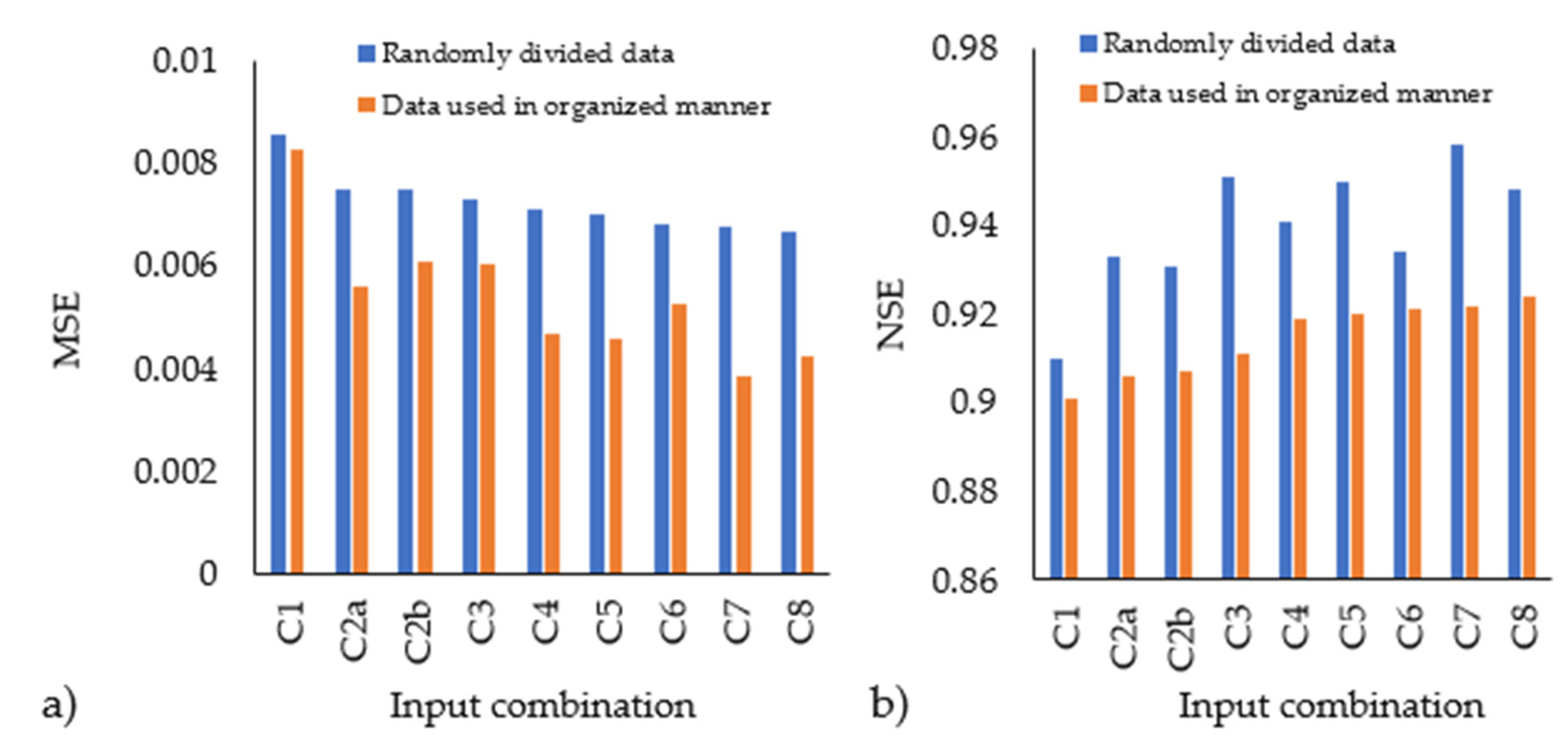
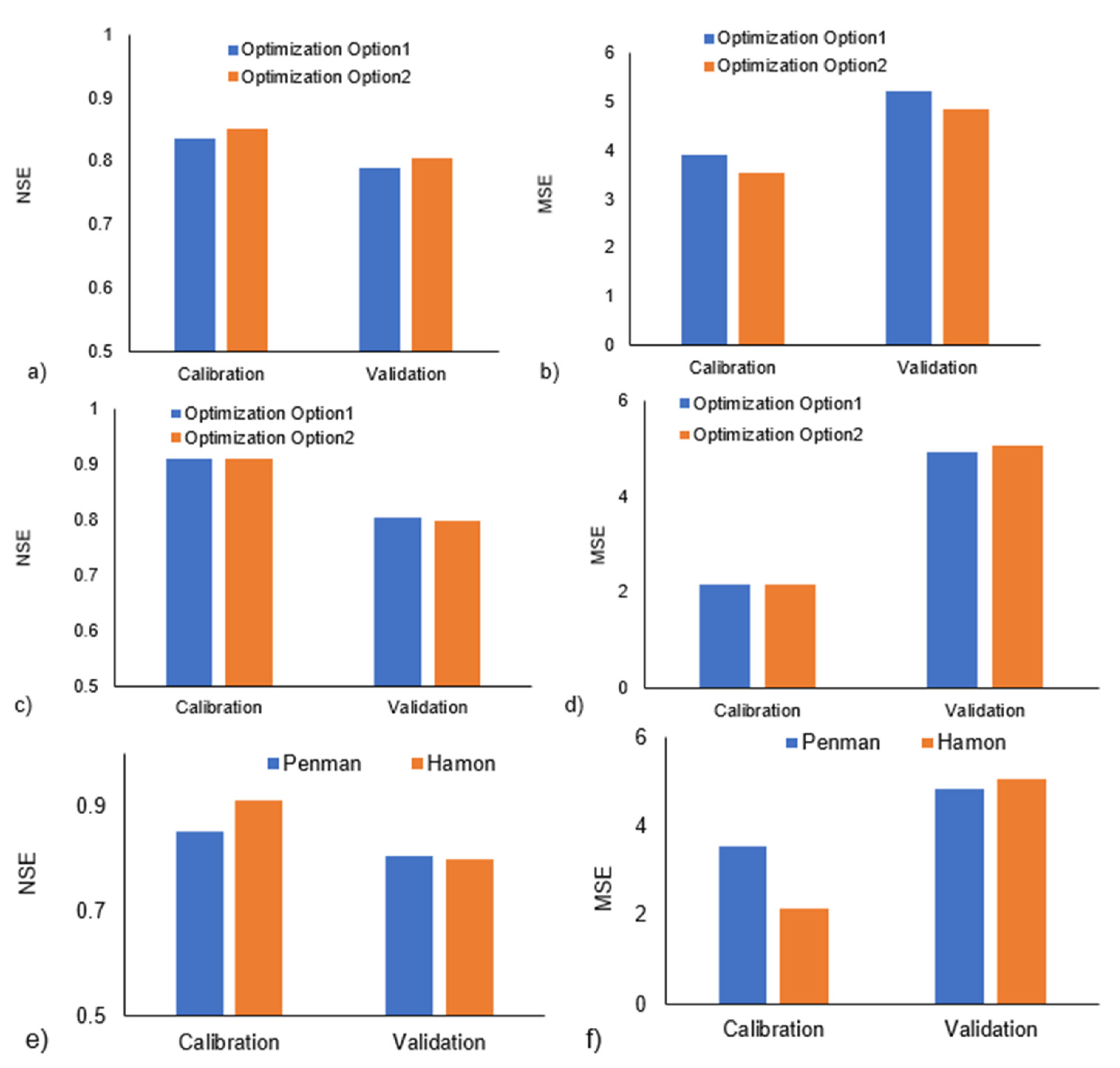
4.4. The Impact Using Various Data Divisions for Training and Testing

Figure 12a,b presents the results of two types of input data divisions used in the ANN-DL-M1 model. It can be observed that training based on randomly divided data results showed better predictions at the stage of validation and testing compared to the case of organizing the first 50% data for training and remaining 50% for validation and testing. The NSE improved by 2 to 4% for various combinations of input parameters. For a fair comparison of models, the remaining work was conducted on the basis of data divided in an organized manner.

4.5. Results of the Prediction of Pan-Evaporation by ANFIS

Figure 13a–c shows the results of the prediction of pan-evaporation by the ANFIS model. The results are highly promising. The MSE is very low and an NSE value of up to 0.97 was achieved. Zounemat-Kermani et al. [57] also obtained highly accurate results for modeling evaporation using ANFIS. As mentioned in Section 3, the ANFIS applies a hybrid-learning rule merging gradient descent, backpropagation, and a least-squares algorithm for estimating a set of parameters. As per the findings of the present study, ANFIS has been proven to be a receptive mathematical structure which can predict a large class of complex-nonlinear-systems (evaporation) with a high degree of accuracy. Various combinations of inputs produced logical and consistent results for predicting pan-evaporation. The error MSE reduces systematically with an increase in the input variables and the NSE value increases with the same pattern as the number of input variables is increased.

4.6. Results of the Prediction of Pan-Evaporation by Penman and Hamon’s Equations

Figure 14a–f shows the comparison of results for Penman and Hamon’s equations. It can be seen in the figure that both the equations successfully predicted the pan-evaporation. These results were obtained on the basis of maximizing the NSE as an objective function. Two different objective functions-MSE (minimized) and NSE (maximized)—in the optimization of parameters of Penman and Hamon’s equations, produced dissimilar results. An NSE value that was about 27% higher in the validation stage was found in the case of the objective function based on NSE compared to its value obtained on the basis of minimizing the objective function (MSE). The results shown in Figure 14 are based on parameter optimization for option-1 and option-2. In option-1, the global maximum values of the objective function were obtained with the constants B₁, B₂, and B₃, as 2.38, 1.75, and 6.86, instead of 0.63, 2.0, and 7.5, respectively.

While identifying the parameters of the Penman Equation, the albedo coefficient (α) was identified as 0.163, instead of 0.26, and the value of 0.54 of constant A₂ was replaced with 0.728. The optimization process revealed that the value of the albedo coefficient significantly impacted the estimated evaporation by Penman Equation. The best possible value of Albedo coefficient was found to be 0.163 with the help of GRG optimization using the data available from three stations of Qassim Region. These results completely match with those of Ghumman et al. [17]. As stated in the methodology, a fair comparison of both the equations can be made if both equations are optimized for same number of parameters (Option-2: two parameters to be optimized for each equation). It was noticed that by decreasing the number of parameters from three to two in case of Hamon’ equation, the efficiency slightly reduced at validation stage, i.e., NSE changed from 0.804 to 0.798. The two parameters produced a global maximum value of NSE for the constants B₁ = 2.88 and B₃ = 6.03, instead of their original values of B₁ = 7.5 and B₃ = 0.63. The results of Option-2 (constants A₁ and A₂ chosen for optimization instead of α and A₂) for Penman Equation showed that the NSE value improved from 0.791 to 0.806. The global maximum value of NSE was obtained for the two parameter values A₁ and A₂ as 15.935 and 0.189 instead of 6.43 and 0.54. The values seem logical. According to the structure of Penman equation (Equation (1)), the wind speed constant (A₁) and the coefficient, before the adventive part of equation (A₂), can be negatively correlated during optimization. The coefficient A₁ before the adventive part of Equation (1) increased by about 2.5 times and the wind function A₂ decreased by about half. These results show a negative correlation amongst the coefficients.

Two different objective functions, MSE (minimized) and NSE (maximized), in the optimization of parameters of Penman and Hamon’s Equations, produced different results. About 27% higher value of NSE in the validation stage was found in the case of the objective function based on NSE as compared to its value obtained on the basis of minimizing the objective function (MSE). The results show that the global minimum/maximum values of objective function are obtained for the values of constants B₁ = 2.38, B₂ = 1.75 and B₃ = 6.86 for Qassim Region instead of B₁ = 0.63, B₂ = 2 and B₃ = 7.5 usually used in the original Hamon’s Equation. Similarly, the Albedo coefficient of α = 0.163 and the wind speed constant A₂ = 0.728 have been identified instead of 0.26 and 0.54 respectively, while identifying the parameters of the Penman Equation. The process of optimization showed that the albedo coefficient significantly changed the evaporation values estimated by the Penman Equation. The best possible value of the albedo coefficient found with the help of GRG optimization is 0.163 for the Qassim Region. These results completely match with those of Ghumman et al. [17].

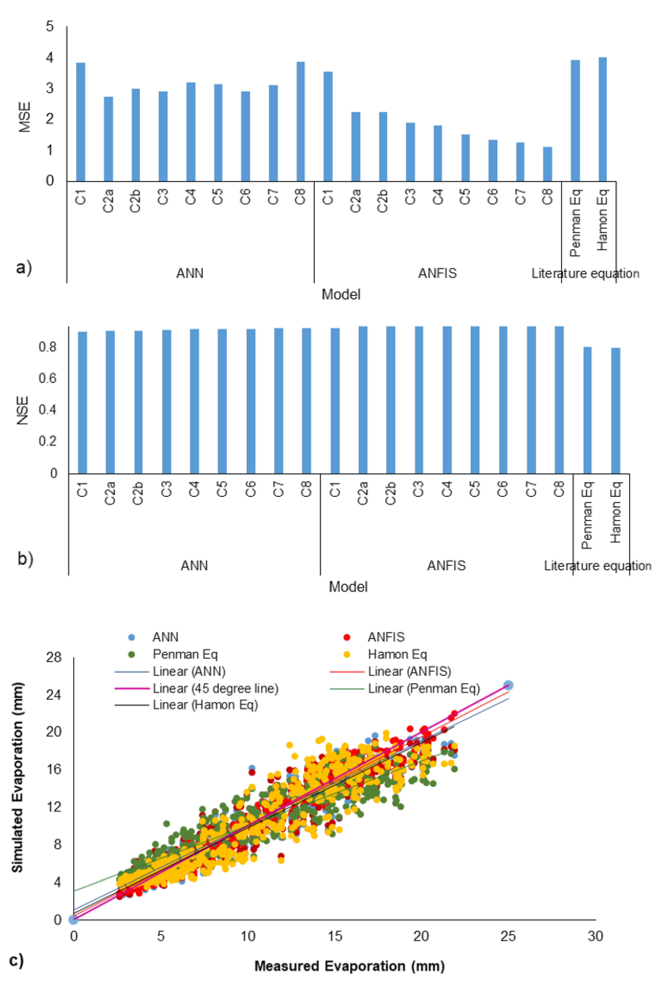
4.7. Comparison of Resuls of Penman and Hamon’s Equations with ANN and ANFIS

Figure 15a–c shows the comparison of results from two types of soft computing models (DL-ANN-M1 and ANFIS) and two Penman and Hamon’s equations. It can be observed that all three techniques were applied successfully to predict the pan-evaporation. MSE is slightly higher as it is calculated on the basis of the whole record containing 480 data points. It is based on real records and not on the normalized values, as estimated in case of the previous figures for ANN and ANFIS. However, the NSE value is promising for all three types of models. None of the NSE values are less than 0.8, which represents a “very good performance” [54,55].

Although the Penman and Hamon’s equations and soft computing models are data-dependent, we have included, to some extent, the physical process involved in the phenomenon of evaporation. We have used the temperature, wind speed, sun shine hours, and net radiation as input data in some combinations of inputs of soft computing models. The Penman Equation also uses the temperature, wind speed, sun shine hours, and net radiation as inputs. Based on the mass-transfer and energy-budget approaches, the equation combines both the fixed bulk surface resistance and vapor aerodynamics [58]. While comparing the three types of models, the performance of both soft computing models is comparatively higher than that of the Penman and Hamon equations. The minimum value of NSE in the case of soft computing models is 0.936, whereas the NSE value for Penman and Hamon’s equations is 0.837 and 0.8, respectively. The Hamon’s Equation only includes two input parameters, but the Penman Equation uses many input parameters, including the temperature, sun shine hours, wind speed, and net radiation, etc. It takes into consideration the fixed-bulk-surface-resistance and vapor aerodynamic (both the energy-budget and mass-transfer approaches are combined together, implicitly generating a solid theoretical basis for estimations of evaporation). However, there is a significant enhancement in the performance if we use the soft computing models in comparison to the Penman and Hamon equations. Among the soft computing models, the performance of ANFIS is outstanding compared to the ANN. A value of NSE equal to 0.972 was achieved by ANFIS, in comparison to a value of 0.958 achieved by ANN.

5. Discussion

A large amount of data measured in the Qassim Region, comprising the pan-evaporation, relative humidity, temperature, and sunshine duration, was used to develop the pan-evaporation estimation models. Three different types of pan-evaporation models were developed, including ANN, ANFIS, and Penman and Hamon’s equations. The results of the three models were compared on the basis of extensive measured data, as mentioned above. The two statistical parameters of MSE and NSE were used for an assessment of the performance of models. Graphs of predicted and measured evaporation data were drawn, where the scatter of data around the 1:1 line was used as a means of comparing the performance of the models.

Various combinations of input variables were tested and it was found that increasing the number of variables increases the efficiency of ANN and ANFIS models. For example, the combinations C2a and C2b include two variables as the input. One combination includes the wind speed with the mean temperature and the other includes the relative humidity with the mean temperature as an input variable. It enhances the performance of ANN and ANFIS in simulating the pan-evaporation compared to the combination with only one variable (temperature) as the input. The enhanced performance of ANN and ANFISS due to such input combinations is logical, because it reflects the adoption of the real physical phenomenon of evaporation, in which the role of the wind speed and relative humidity is quite pronounced. In advanced countries, all parameters used in various combinations of input variables adopted in this study are measured. However, in the present study, combinations with more than four variables as the input resulted in overfitting because the four measured variables were used to determine the remaining four variables, so the impact of several variables is repeated in combinations with more than four variables.

The identification of the best possible values of parameters of Penman and Hamon’s equations using GRG optimization was conducted on the basis of two different objective functions, including MSE and NSE. Maximizing the objective function based on NSE produced comparatively better results compared to those obtained when the objective function was based on MBE (NSE value 27% higher in the validation stage). Two pan-evaporation models, including Penman and Hamon’s equations, were developed for the Al Qassim Region. The best possible values of constants B₁, B₂, and B₃ in Hamon’s Equation for the Qassim Region were 2.38, 1.75, and 6.86, instead of 0.63, 2, and 7.5 respectively used in the original Hamon’s Equation. In the case of the Penman Equation, the albedo coefficient of 0.163 and the constant 0.728 were identified, instead of the albedo coefficient of 0.26 and wind speed constant 0.54, respectively. It can be concluded that the value of the albedo coefficient had a significant impact on the estimated values of evaporation obtained from the Penman Equation. The albedo coefficient, found with the help of optimization, was 0.163 for the Qassim Region.

The number of parameters identified in the optimization process exhibits significant importance in pan-evaporation simulation. Decreasing the number of parameters from three to two in the case of Hamon’s Equation slightly reduced the efficiency at the validation stage, i.e., the value of the statistical indicator NSE changed from 0.804 to 0.798. The two parameters produced a global maximum value of NSE for the constants B₁ = 2.88 and B₃ = 6.03, instead of their original values of 7.5 and 0.63, respectively, as given in the equation. The parameters of Penman’s Equation can be different for different situations. If the albedo coefficient is very well-known for the region, it should not be used in the optimization. The constant 6.43 can be chosen for optimization instead of the albedo coefficient. For such situations, the optimization of parameters of the Penman Equation showed an improvement of the NSE value from 0.791 to 0.806. The global maximum value of NSE was obtained for the two parameter values of A₁ = 15.935 and A₂ = 0.189, instead of 6.43 and 0.54, respectively, usually found in the original equation.

It might be noted that a general methodology has been developed for the parameter optimization of Penman and Hamon’s equations and the prediction of evaporation by ANN and ANFIS in this research. Although the methodology has been applied using the data from the Qassim Region, it may be applicable for any region worldwide with similar climatic conditions. The results of the study may be of particular interest to practical engineers, decision makers, and planners.

6. Conclusions and Recommendations

ANNs with various architectures were investigated and the results of pan-evaporation were found to be promising for various architectures of ANN using 5, 10, or 15 neurons in hidden layers. The NSE values higher than 0.85 for all cases indicate the high performance of the models. The architecture with 10 neurons in hidden layers simulated comparatively better results of pan-evaporation than those with 5 and 15 neurons. NSE values up to 0.96 could be obtained using 10 neurons in hidden layers of ANN. An architecture with the higher number of neurons in hidden layers of ANN is not preferred.

The ANN models with double and triple hidden layers were tested and it was found that both types of models perform equally well. The maximum value of NSE is 0.963 and the minimum is 0.902. The double layer models are mainly recommended because of their simple nature.

Various combinations of input variables in ANN models produced varying performances for the prediction of pan-evaporation. Although the model with only one input parameter (mean daily temperature) is the simplest, it predicts pan-evaporation with a reasonable accuracy, i.e., MSE values of 0.0065, 0.0069, and 0.0083 and NSE values of 0.923, 0.926, and 0.91 in the training, validation, and testing stages respectively. This type of input is highly suitable for countries with a scarcity of data. The input combination with two variables, including either the wind speed with the mean temperature as an input variable or the relative humidity with the mean temperature, significantly enhances the performance of ANN in simulating the pan-evaporation. MSE values as low as 0.00498, 0.0055, and 0.0056 and NSE values as high as 0.94, 0.934, and 0.933 can be achieved by such an input combination in the training, validation, and testing stages, respectively. The combinations containing three, four, five, six, seven, and eight variables as input parameters produced a relatively higher model efficiency. However, higher numbers of parameters are not always recommended due to the relatively higher complexity of models and the scarcity of recorded data in some arid regions.

The ANFIS model has a high performance in predicting the pan-evaporation, with a very low value of MSE. An NSE value of up to 0.97 can be achieved, which represents an excellent performance. Various combinations of input variables produced logical and consistent results for predicting pan-evaporation with the help of ANFIS. A significant and systematic reduction in error (MSE) and an increase in NSE can be achieved by the application of ANFIS, with an increase in the input variables.

With regard to the comparison of various models developed in this research for the prediction of pan-evaporation, the ANFIS exhibits the first position, ANN second, the Penman Equation third, and Hamon’s Equation fourth, based on the statistical parameters (MSE and NSE) achieved during various applications of the models.

References

1. Tarawneh, Q.Y.; Chowdhury, S. Trends of Climate Change in Saudi Arabia: Implications on Water Resources. Climate 2018, 6, 8. [Google Scholar] [CrossRef] [Green Version]
2. Jafari, M.; Dinpashoh, Y.; Asadi, E.; Darbandi, S. Evaluation of Bayesian Network Model for Estimation of Pan Evaporation. Irrig. Sci. Eng. 2020, 43, 93–106. [Google Scholar]
3. Kumar, N.; Arakeri, J.H. A fast method to measure the evaporation rate. J. Hydrol. 2020, 125642. [Google Scholar] [CrossRef]
4. Li, J.; Wang, C. An Evaporation Correction Approach and Its Characteristics. J. Hydrometeorol. 2020, 21, 519–532. [Google Scholar] [CrossRef]
5. Kumar, N.; Arakeri, J.H. Understanding the coupling between the moisture loss and surface temperature in an evaporating leaf-type surface. Dry. Technol. 2020. [Google Scholar] [CrossRef]
6. Malik, A.; Kumar, A.; Kim, S.; Kashani, M.H.; Karimi, V.; Sharafati, A.; Ghorbani, M.A.; Al-Ansari, N.; Salih, S.Q.; Yaseen, Z.M.; et al. Modeling monthly pan evaporation process over the Indian central Himalayas: Application of multiple learning artificial intelligence model. Eng. Appl. Comput. Fluid Mech. 2020, 14, 323–338. [Google Scholar] [CrossRef] [Green Version]
7. Crago, R.D.; Szilagyi, J.; Qualls, R. Comment on: “A review of the complementary principle of evaporation: From the original linear relationship to generalized nonlinear functions” by Han and Tian (2020). Hydrol. Earth Syst. Sci. 2021, 25, 63–68. [Google Scholar] [CrossRef]
8. Weerasinghe, I.; Bastiaanssen, W.; Mul, M.; Jia, L.; van Griensven, A. Can we trust remote sensing evapotranspiration products over Africa? Hydrol. Earth Syst. Sci. 2020, 24, 1565–1586. [Google Scholar] [CrossRef] [Green Version]
9. Patle, G.T.; Chettri, M.; Jhajharia, D. Monthly pan evaporation modelling using multiple linear regression and artificial neural network techniques. Water Supply 2020, 20, 800–808. [Google Scholar] [CrossRef]
10. Mozny, M.; Trnka, M.; Vlach, V.; Vizina, A.; Potopova, V.; Zahradnicek, P.; Stepanek, P.; Hajkova, L.; Staponites, L.; Zalud, Z. Past (1971–2018) and future (2021–2100) pan evaporation rates in the Czech Republic. J. Hydrol. 2020, 590, 125390. [Google Scholar] [CrossRef]
11. Wang, B.; Ma, Y.; Ma, W.; Su, B.; Dong, X. Evaluation of Ten Methods for Estimating Evaporation in a Small High-Elevation Lake on the Tibetan Plateau. Appl. Clim. 2019, 136, 1033–1045. [Google Scholar] [CrossRef]
12. Ahmadipour, A.; Shaibani, P.; Mostafavi, S.A. Assessment of Empirical Methods for Estimating Potential Evapotranspiration in Zabol Synoptic Station by REF-ET Model. Medbiotech J. 2019, 3, 1–4. [Google Scholar]
13. Zolá, R.P.; Bengtsson, L.; Berndtsson, R.; Martí-Cardona, B.; Satgé, F.; Timouk, F.; Bonnet, M.P.; Mollericon, L.; Gamarra, C.; Pasapera, J. Modelling Lake Titicaca’s Daily and Monthly Evaporation. Hydrol. Earth Syst. Sci. 2019, 23, 657–668. [Google Scholar] [CrossRef] [Green Version]
14. Benabdelouahab, T.; Lebrini, Y.; Boudhar, A.; Hadria, R.; Htitiou, A.; Lionboui, H. Monitoring spatial variability and trends of wheat grain yield over the main cereal regions in Morocco: A remote-based tool for planning and adjusting policies. Geocarto Int. 2019. [Google Scholar] [CrossRef]
15. Talbot, M. Comparison of Evapotranspiration Estimation Methods and Implications for Water Balance Model Parameterization in the Midwestern United States. Retrieved from the University of Minnesota Digital Conservancy. 2019. Available online: https://hdl.handle.net/11299/211721 (accessed on 26 December 2020).
16. Mahmoud, S.H.; Gan, T.Y. Irrigation water management in arid regions of Middle East: Assessing spatio-temporal variation of actual evapotranspiration through remote sensing techniques and meteorological data. Agric. Water Manag. 2019, 212, 35–47. [Google Scholar] [CrossRef]
17. Ghumman, A.R.; Ghazaw, Y.M.; Alodah, A.; ur Rauf, A.; Shafiquzzaman, M.; Haider, H. Identification of Parameters of Evaporation Equations Using an Optimization Technique Based on Pan Evaporation. Water 2020, 12, 228. [Google Scholar] [CrossRef] [Green Version]
18. Han, S.; Tian, F. A review of the complementary principle of evaporation: From the original linear relationship to generalized nonlinear functions. Hydrol. Earth Syst. Sci. 2020, 24, 2269–2285. [Google Scholar] [CrossRef]
19. Hadria, R.; Benabdelouhab, T.; Lionboui, H.; Salhi, A. Comparative assessment of different reference evapotranspiration models towards a fit calibration for arid and semi-arid areas. J. Arid Environ. 2021, 184, 104318. [Google Scholar] [CrossRef] [PubMed]
20. Alsumaiei, A.A. Utility of Artificial Neural Networks in Modeling Pan Evaporation in Hyper-Arid Climates. Water 2020, 12, 1508. [Google Scholar] [CrossRef]
21. Haghbin, M.; Sharafati, A.; Motta, D.; Al-Ansari, N.; Noghani, M.H.M. Applications of soft computing models for predicting sea surface temperature: A comprehensive review and assessment. Prog. Earth Planet. Sci. 2020, 8, 4. [Google Scholar] [CrossRef]
22. Bruton, J.M.; McClendon, R.W.; Hoogenboom, G. Estimating daily pan evaporation with artificial neural networks. Trans. Asae 2000, 43, 491. [Google Scholar] [CrossRef]
23. Sudheer, K.P.; Gosain, A.K.; Ramasastri, K.S. Estimating actual evapotranspiration from limited climatic data using neural computing technique. J. Irrig. Drain. Eng. 2003, 129, 214–218. [Google Scholar] [CrossRef]
24. Traore, S.; Wang, Y.-M.; Kerh, T. Artificial neural network for modeling reference evapotranspiration complex process in Sudano-Sahelian zone. Agric. Water Manag. 2010, 97, 707–714. [Google Scholar] [CrossRef]
25. Qasem, S.N.; Samadianfard, S.; Kheshtgar, S.; Jarhan, S.; Kisi, O.; Shamshirband, S.; Chau, K.-W. Modeling monthly pan evaporation using wavelet support vector regression and wavelet artificial neural networks in arid and humid climates. Eng. Appl. Comput. Fluid Mech. 2019, 13, 177–187. [Google Scholar] [CrossRef] [Green Version]
26. Chaudhari, N.; Londhe, S.; Khare, K. Estimation of pan evaporation using soft computing tools. Int. J. Hydrol. Sci. Technol. 2012, 2, 373–390. [Google Scholar] [CrossRef]
27. Ghorbani, M.A.; Deo, R.C.; Yaseen, Z.M.; Kashani, M.H.; Mohammadi, B. Pan evaporation prediction using a hybrid multilayer perceptron-firefly algorithm (MLP-FFA) model: A case study in North Iran. Theor. Appl. Climatol. 2018, 133, 1119–1131. [Google Scholar] [CrossRef]
28. Majhi, B.; Naidu, D. Pan evaporation modeling in different agro-climatic zones using functional link artificial neural network. Inf. Process. Agric. 2020, 8, 134–147. [Google Scholar] [CrossRef]
29. Keskin, M.E.; Terzi, Ö. Artificial neural network models of daily pan evaporation. J. Hydrol. Eng. 2006, 11, 65–70. [Google Scholar] [CrossRef]
30. Kumar, M.; Raghuwanshi, N.S.; Singh, R. Artificial neural networks approach in evapotranspiration modeling: A review. Irrig. Sci. 2011, 29, 11–25. [Google Scholar] [CrossRef]
31. Zhang, M.; Su, B.; Nazeer, M.; Bilal, M.; Qi, P.; Han, G. Climatic Characteristics and Modeling Evaluation of Pan Evapotranspiration over Henan Province, China. Land 2020, 9, 229. [Google Scholar] [CrossRef]
32. Nourani, V.; Elkiran, G.; Abdullahi, J. Multi-station artificial intelligence based ensemble modeling of reference evapotranspiration using pan evaporation measurements. J. Hydrol. 2019, 577, 123958. [Google Scholar] [CrossRef]
33. Dou, X.; Yang, Y. Evapotranspiration estimation using four different machine learning approaches in different terrestrial ecosystems. Comput. Electron. Agric. 2018, 148, 95–106. [Google Scholar] [CrossRef]
34. Winter, T.C.; Rosenberry, D.O.; Sturrock, A.M. Evaluation of 11 Equations for Determining Evaporation for a Small Lake in The North Central United States. Water Resour. Res. 1995, 31, 983–993. [Google Scholar] [CrossRef]
35. Penman, H.L. Natural Evaporation from Open Water, Bare Soil, and Grass. Proc. R. Soc. 1948, 76, 372–383. [Google Scholar]
36. Valiantzas, J.D. Simplified Version for The Penman Evaporation Equation Using Routine Weather Data. J. Hydrol. 2006, 331, 690–702. [Google Scholar] [CrossRef]
37. Doorenbus, J.; Pruitt, W.O. Guidelines for Predicting Crop Water Requirements, Irrigation and Drainage Paper; Food and Agriculture Organization of the United Nations: Rome, Italy, 1977. [Google Scholar]
38. Alazrd, M.; Leduc, C.; Travi, Y.; Boulet, G.; Ben Salem, A. Estimating Evaporation in Semi-Arid Areas Facing Data Scarcity: Examples of the El Haouraeb Dam (Merguellil catchment, Central Tunisia). J. Hydrol. Reg. Stud. 2015, 3, 265–284. [Google Scholar] [CrossRef] [Green Version]
39. Souch, C.; Wolfe, C.P.; Susan, C.; Grimmond, B. Wetland Evaporation and Energy Partitioning: Indiana Dunes National Lakeshore. J. Hydrol. 1996, 184, 189–208. [Google Scholar] [CrossRef]
40. Yao, H.; Terakawa, A.; Chen, S. Rice Water Use and Response to Potential Climate Changes: Calculation and Application to Jianghan, China. In Proceedings of the International Conference on Water Resources and Environment Research, Kyoto, Japan, 5–9 June 1996; Volume 2, pp. 611–618. [Google Scholar]
41. Shuttleworth, W.J. Putting the “Vap” in Evaporation. Hydrol. Earth Syst. Sci. 2007, 11, 210–244. [Google Scholar] [CrossRef] [Green Version]
42. Vardavas, I.M. Modeling the Seasonal Radiation of Net All-Wave Radiation Flux and Evaporation in a Tropical Wet-Dry Region. Ecol. Model. 1987, 39, 247–268. [Google Scholar] [CrossRef]
43. Vardvas, I.M.; Fountoulakis, A. Estimation of Lake Evaporation from Standard Meteorological Measurements: Application to Four Australian Lakes in Different Climatic Regions. Ecol. Modell. 1996, 84, 139–150. [Google Scholar] [CrossRef]
44. Maghrabi, A.H.; Al-Mostafa, Z.A. Estimating surface albedo over Saudi Arabia. Renew. Energy 2009, 34, 1607–1610. [Google Scholar] [CrossRef]
45. Hamon, W.R. Estimating Potential Evapotranspiration. J. Hydraul. Div. Proc. Am. Soc. Civ. Eng. 1963, 871, 107–120. [Google Scholar]
46. Morton, F.I. Catchment Evaporation and Potential Evaporation Further Development of a Climatological Relationship. J. Hydrol. 1971, 12, 81–99. [Google Scholar] [CrossRef]
47. Zhou, Y.; Yang, B.; Han, J.; Huang, Y. Robust Linear Programming and Its Application to Water and Environmental Decision-Making under Uncertainty. Sustainability 2019, 11, 33. [Google Scholar] [CrossRef] [Green Version]
48. Sheela, K.G.; Deepa, S.N. Review on Methods to Fix Number of Hidden Neurons in Neural Networks. Math. Probl. Eng. 2013, 2013, 425740. [Google Scholar] [CrossRef] [Green Version]
49. Peterson, C.; Rognvaldsson, T. An Introduction to Artifical Neuron Network; Departement of Theoretical Physic, Cern School of Computing: Ystad, Sweden, 1991. [Google Scholar]
50. Arifin, F.; Robbani, H.; Annisa, T.; Ma’arof, N.N.M.I. Variations in the Number of Layers and the Number of Neurons in Artificial Neural Networks: Case Study of Pattern Recognition. J. Phys. Conf. Ser. 2019, 1413, 012016. [Google Scholar] [CrossRef] [Green Version]
51. Ogunbo, J.N.; Alagbe, O.A.; Oladapo, M.I.; Shin, C. N-hidden layer artificial neural network architecture computer code: Geophysical application example. Heliyon 2020, 6, 04108. [Google Scholar] [CrossRef] [PubMed]
52. Almuhaylan, M.R.; Ghumman, A.R.; Al-Salamah, I.S.; Ahmad, A.; Ghazaw, Y.M.; Haider, H.; Shafiquzzaman, M. Evaluating the Impacts of Pumping on Aquifer Depletion in Arid Regions Using MODFLOW, ANFIS and ANN. Water 2020, 12, 2297. [Google Scholar] [CrossRef]
53. Nash, J.E.; Sutcliffe, J.V. River Flow Forecasting Through Conceptual Models, Part I—A Discussion of Principles. J. Hydrol. 1970, 10, 282–290. [Google Scholar] [CrossRef]
54. Moriasi, D.N.; Arnold, J.G.; Liew, V.M.W.; Bingner, R.L.; Harmel, R.D.; Veith, T.L. Model evaluation guidelines for systematic quantification of accuracy in watershed simulations. Am. Soc. Agric. Biol. Eng. 2007, 50, 885–900. [Google Scholar]
55. Rauf, A.; Ghumman, A.R. Impact Assessment of Rainfall-Runoff Simulations on the Flow Duration Curve of the Upper Indus River—A Comparison of Data-Driven and Hydrologic Models. Water 2018, 10, 876. [Google Scholar] [CrossRef] [Green Version]
56. Garces-Jimenez, A.; Castillo-Sequera, J.L.; Corte-Valiente, A.D.; Gómez-Pulido, J.M.; González-Seco, E.P.D. Analysis of Artificial Neural Network Architectures for Modeling Smart Lighting Systems for Energy Savings. IEEE Access 2019, 7, 119881–119891. [Google Scholar] [CrossRef]
57. Zounemat-Kermani, M.; Kisi, O.; Piri, J.; Mahdavi-Meymand, A. Assessment of Artificial Intelligence–Based Models and Metaheuristic Algorithms in Modeling Evaporation. J. Hydrol. Eng. 2020, 24, 199886595. [Google Scholar] [CrossRef]
58. Tukimat, N.N.A.; Harun, S.; Shahid, S. Comparison of Different Methods in Estimating Potential Evapotranspiration at Muda Irrigation Scheme of Malaysia. J. Agric. Rural Dev. Trop. Subtrop. 2012, 113, 77–85. [Google Scholar] [CrossRef]
Figure 1. Map highlighting the Qassim Region location in Saudi Arabia.
Water 13 00793 g001
Figure 2. Daily values of measured meteorological parameters (average for the period 1976–2016): (a) Evaporation; (b) temperature; (c) relative humidity; (d) sunshine hours; and (e) wind speed.
Water 13 00793 g002
Figure 3. Framework for the methodology.
Water 13 00793 g003
Figure 5. Various input combinations used for ANN simulations.
Water 13 00793 g005
Figure 6. Five functional blocks in the Artificial Neuro Fuzzy Inference System (ANFIS) (after Almohaylan et al. [52]).
Water 13 00793 g006
Figure 7. Comparison of the various architecture of double layer (DL)-ANN models with 5, 10, and 15 hidden neurons.
Water 13 00793 g007
Figure 8. Comparison of DL- and triple layer (TL)-ANN models (M1 to M5) with 10 hidden neurons, (a) Mean Square Error (MSE) comparison, and (b) Nash and Sutcliffe Efficiency (NSE) bar graph.
Water 13 00793 g008
Figure 9. Performance results of DL-ANN models (M1 to M5) with 10 hidden neurons, (a) M1-Levenberg–Marquardt BP, (b) M2- Bayesian regularization, (c) M3- BFGS Quasi-Newton BP and M4- Resilient backpropagation (Rprop), (d) M5- Scaled conjugate gradient BP.
Water 13 00793 g009
Figure 10. Comparison of DL- and TL-ANN models (M1-M5) with 10 hidden neurons, Comparison based on trend lines: (a) Trend lines of DL models (M1–M5) in comparison with the 45° line; (b) trend lines of TL models (M1-M5) in comparison with the 45° line; and (c) trend lines of the DL and TL model for the best training function (M1) in comparison with the 45° line.
Water 13 00793 g010
Figure 11. ANN-DL-M1-model results for the prediction of evaporation with 10 hidden neurons (the impact of various input combinations): (a) MSE; (b) NSE; and (c) measured vs. predicted evaporation.
Water 13 00793 g011
Figure 12. Comparison of DL-ANN-M1 model results for various data divisions with 10 hidden neurons used for training, validation, and testing: (a) MSE and (b) NSE.
Water 13 00793 g012
Figure 13. ANFIS model results for the prediction of pan-evaporation: (a) MSE; (b) NSE; and (c) measured vs. predicted evaporation.
Water 13 00793 g013
Figure 14. The results Penman and Hamon’s Equations: (a) NSE values for Penman Equation Results, (b) MSE values for Penman Equation Results, (c) NSE values for Hamon’ Equation Results, (d) MSE values for Hamon’ Equation Results, (e) NSE values for comparison of Penman and Homan’s Equation Results, (f) MSE values for comparison of Penman and Homan’s Equation Results.
Water 13 00793 g014
Figure 15. Comparison of DL-ANN-M1, ANFIS, and Penman and Hamon’s equations for modeling pan-evaporation: (a) MSE; (b) NSE; and (c) 45° line.
Water 13 00793 g015