Article

Estimation of the Climate Change Impact on the Hydrological Balance in Basins of South-Central Chile

by
Rebeca Martínez-Retureta
1,2,*,
Mauricio Aguayo
1,2,*,
Norberto J Abreu
3,4,*,
Alejandra Stehr
1,5,
Iongel Duran-Llacer
1,2,
Lien Rodríguez-López
1,
Sabine Sauvage
6 and
José-Miguel Sánchez-Pérez
6
1
Environmental Sciences Center EULA-Chile, University of Concepción, Concepción 4070386, Chile
2
Territorial Planning Department, Faculty of Environmental Science, University of Concepción, Concepción 4070386, Chile
3
Center of Waste Management and Bioenergy, Scientific and Technological Bioresources Nucleus, Universidad de la Frontera, Casilla 54-D, Temuco 4780000, Chile
4
Department of Chemical Engineering, Faculty of Engineering and Sciences, Universidad de la Frontera, Casilla 54-D, Temuco 4780000, Chile
5
Environmental Engineering Department, Faculty of Environmental Science, University of Concepción, Concepción 4070386, Chile
6
ECOLAB, University of Toulouse, CNRS, INPT, UPS, 31326 Auzeville-Tolosane, France
*
Authors to whom correspondence should be addressed.
Water 2021, 13(6), 794; https://doi.org/10.3390/w13060794
Submission received: 3 February 2021 / Revised: 22 February 2021 / Accepted: 5 March 2021 / Published: 14 March 2021
(This article belongs to the Special Issue Climate Change Impacts on Water Resources)

Abstract

:
In this study, the SWAT (Soil Water Assessment Tool) hydrological model is implemented to determine the effect of climate change on various hydrological components in two basins located in the foothills of the Andes: the Quino and Muco river basins. The water cycle is analyzed by comparing the model results to climatic data observed in the past (1982–2016) to understand its trend behaviors. Then, the variations and geographical distribution of the components of the hydrological cycle were analyzed using the Representative Concentration Pathway (RCP)8.5 climate scenario to model two periods considering the immediate future (2020–2049) and intermediate future (2050–2079). In this way, in the study area, it is predicted that yearly average temperatures will increase up to 1.7 °C and that annual average precipitation will decrease up to 210 mm for the intermediate future. Obtained results show that the analyzed parameters presented the same trend behavior for both periods of time; however, a greater impact can be expected in the intermediate future. According to the spatial distribution, the impact worsens for all the parameters as the elevation increases in both basins. The model depicted that yearly average evapotranspiration would increase around 5.26% and 5.81% for Quino and Muco basins, respectively, due to the large increase in temperature. This may cause, when combined with the precipitation lessening, a decrease around 9.52% and 9.73% of percolation, 2.38% and 1.76% of surface flow, and 7.44% and 8.14% of groundwater for Quino and Muco basins, respectively, with a consequent decrease of the water yield in 5.25% and 4.98% in the aforementioned watersheds, respectively.

1. Introduction

Climate change and the effect of anthropic alterations on the hydrological cycle have achieved considerable interest in the scientific community. Several impacts of climate change can be predicted through the variation in the hydrological cycle [1,2]. Strong evidence showing that climate change is altering hydrological cycles at the regional and global levels has been exposed [3,4], indicating consistent predicted effects: changes in precipitation patterns, increased intensity of extreme weather events, glacier retreat and its consequent alterations in the river discharge regimes [4].
The temperature increases and rainfall fluctuations predicted could have an effect on evaporation from the soil and plant transpiration, contributing to the emission of water vapor into the atmosphere. This increase in water vapor could change the frequency and distribution of rainfall, thus affecting surface runoff and groundwater recharge regimes in the future [5,6]. Such changes could also increase the vulnerability of water systems, known as their susceptibility to damage or lack of adaptation capacity [4]. Therefore, the understanding of present and projected global climatic conditions becomes relevant in the determination of vulnerabilities and the development of adaptation strategies to climate change.
In order to assess climate evolution, under different anthropogenic forcing factors, such as greenhouse gas emissions, the general circulation models (GCM) are the most reliable tools providing estimations of possible future climates based on socio-economic and demographic factors according to different emission scenarios. GCMs often apply representative concentration pathways (RCP) for future climate models. Such RCPs are derived from innovative multidisciplinary collaboration with integrated assessment modelers, terrestrial ecosystem and climate modelers, and emissions inventory experts [7], among others.
As established by the United Nations Framework Convention on Climate Change (UNFCCC) [8], mountain areas are highly vulnerable to climate change, complying with seven of the nine vulnerability criteria. In this context, Andean mountain and particularly Chile is a diverse country from the orographic and physical points of view. Its latitude, altitude, the influence of the Pacific Ocean and its continentality are some the main climatic drivers of the region. Additionally, it is affected by factors such as the influence of the Amazon in the north, the westerly winds in the south and the Humboldt current system driven by the South Pacific Subtropical High [9,10,11].
Climate variability studies performed in Chile for the XXI century by the Chilean National Commission for the Environment of the Geophysical Department, University of Chile (CONAMA-DGF), [12] depict that, for the south-central zone of Chile, the rainfall regime has experienced a decreasing trend since the mid-1970s. The report also indicates the decrease in rainfall as well as an increase in temperatures in most of the territory during the coming years.
Moreover, studies performed in 2011 by the Geophysics Department of the University of Chile [13] highlight a behavior in the central-south zone, characterized by a sustained trend for several decades. On one hand, the annual average temperature for different sets of stations in the ocean and along the coast have decreased by −0.15 °C per decade; meanwhile, the central valley stations unveil a temperature increase in the mountain range about 0.25 °C per decade [13]. On the other hand, in the south-central region of Chile, long-term climatic studies indicate a decrease in precipitation along with higher temperatures, greater climatic variability and hydrological drought [14,15,16,17].
Recent studies [18,19,20] have implemented physically based distributed hydrological models driven by GCMs to understand the impact of climate change on the hydrological process at the basin scale. The Soil Water Assessment Tool (SWAT) is a hydrological modeling tool used to simulate and predict hydrological processes. Nowadays, this model has been widely used by the international scientific community [21]. SWAT allows the incorporation of the effect of climate change into the simulation [22,23].
It has been stated that water resources at the pre-cordilleran basins of south-central Chile could be significantly affected during the next century due to global climate change [24]. This study focuses on understanding the impacts of climate change on the components of the hydrological cycle in basins of south-central Chile. In this way, useful information is provided for the design of basin management strategies and regional adaptation policies that could contribute to the mitigation of the climate change effect on water resources. Quino and Muco basins were selected considering hydro-meteorological data availability of, at least, a 35-year time series. Such basins have undergone important climatic variations over the last decades.
The study objectives are first to analyze the annual variation of the hydro-meteorological components over the last 35 years. Furthermore, the prediction of the response of the hydrological cycle according to the immediate future (2020–2049) and intermediate future (2050–2079) climate scenarios is assessed.

2. Materials and Methods
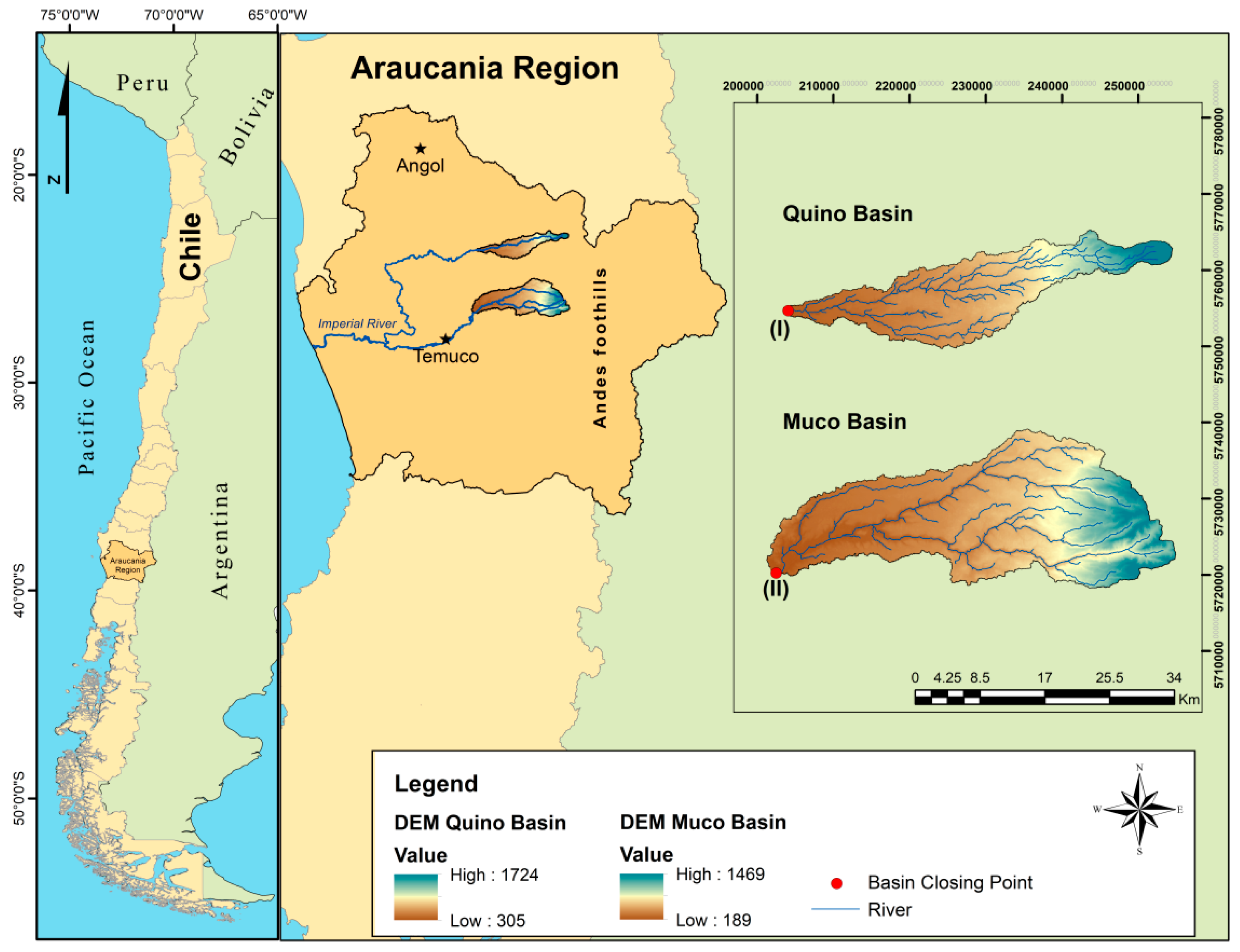
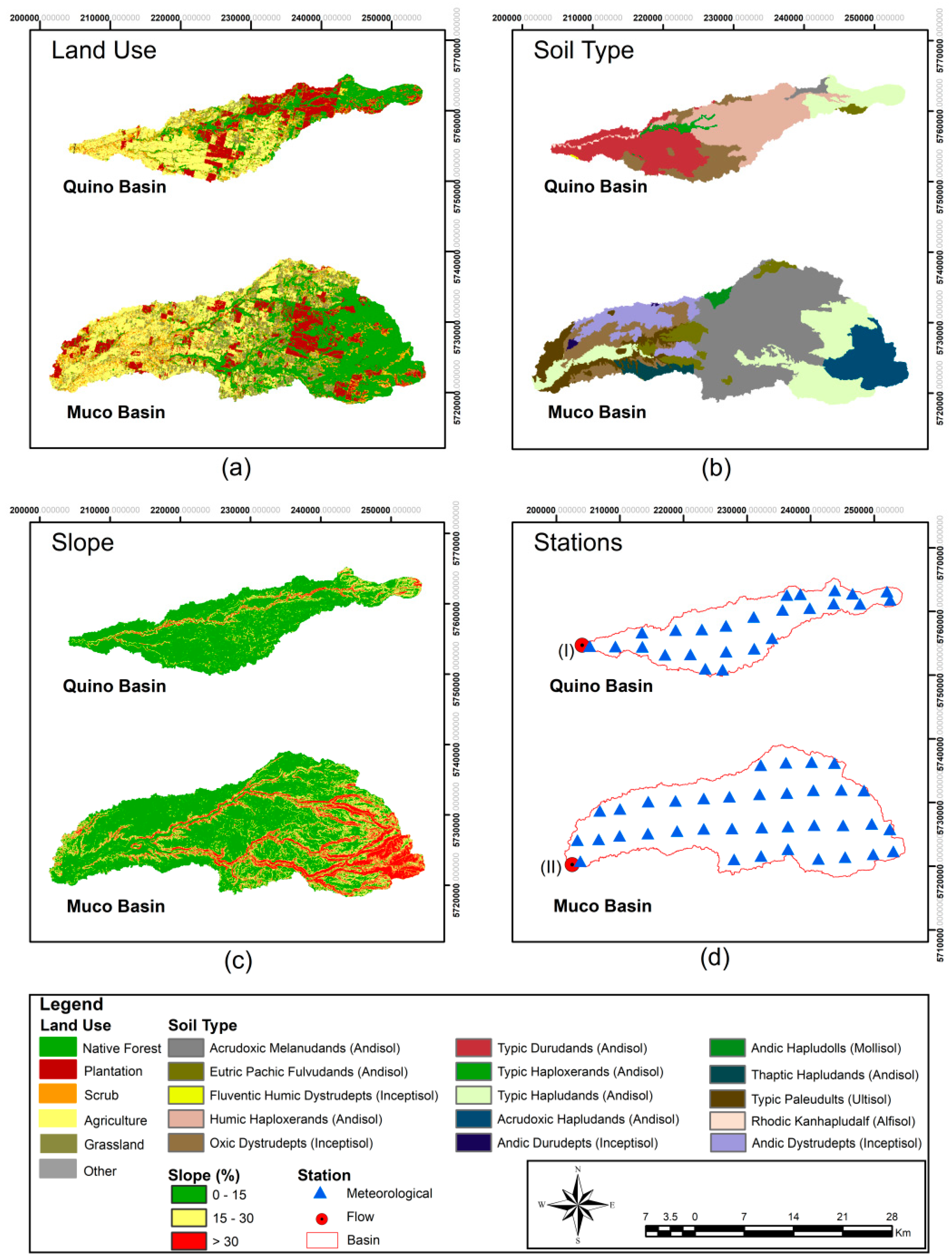
2.1. Study Areas

Quino and Muco basins are located in the Araucanía Region, in the south-central zone of Chile (38°10′00″ S and 38°40′00″ S) (Figure 1). This zone supports an important industrial development strongly related to forestry and agricultural production, also linked to hydroelectric generation. It is located on the border of two significant eco-regions for world conservation, the Mediterranean Scrub and the temperate rainforest, within the biodiversity hotspot called Valdivian Rainforest [25].
Selected pre-cordilleran hydrographic systems, Quino and Muco basins, have 299 and 651 km2 of area and elevations ranging from 305 to 1724 mamsl and from 189 to 1469 mamsl, respectively. The basins are located in a transition area between Mediterranean dominance and temperate humid conditions [26]. Annual average precipitations in the basins vary between 1253 mm and 2693 mm and annual average temperatures between 10 °C and 12 °C.

2.2. Hydrological Modelling

2.2.1. Model Description

The SWAT model (Texas A&M University, Texas, USA, Version 2012.10.4.21) allows simulating several physical processes concerning the hydrological cycle at different time scales. The model presents three different ways to discretize the basin: grids, slopes and sub-basins schemes [27]. In this work, the monthly time scale and the sub-basin scheme derived from the digital elevation model (DEM) were approached. Thereby, sub-basin configuration considers the preservation of the channels and the natural flow path within the model. Firstly, the waterways were defined, opting to create them from the minimum area threshold automatically established by SWAT, achieving an accurate representation of the channels.
Next, a hydrologic response units (HRUs) discretization method was also applied in order to improve the simulation accuracy. HRUs were obtained by integrating the soil type, land use and slope. This method allows reflecting more accurately the spatial variability of the process through which rain transforms into runoff, as well as the routing of the water in each HRU [28].
Additionally, daily climatic information on precipitation and maximum and minimum temperatures was incorporated to calculate the main processes of the hydrological cycle, using the Hargreaves method [29] to determine the potential evapotranspiration.

2.2.2. Databases

The input data for SWAT hydrological model were obtained using the Geographic Information System ArcGIS, ArcMap 10.4. (ESRI Geographic Information System Company, California, USA) The DEM was developed using Alos-1 Palsar sensor images with a spatial resolution of 12.5 m (https://vertex.daac.asf.alaska.edu/, accessed on 12 November 2020). Soil type information was obtained from the agrological studies of the IX Region performed by the Natural Resources Information Center (CIREN) in 2002 for the Araucanía region [30]. The aforementioned study provides information about the soil types present on the study area and their associated physical–chemical properties. This information was included in the database used in the SWAT model for the hydrological simulations [28]. Land use and coverage data for Muco and Quino basins for 2011 were acquired from satellite image processing carried out by Heilmayr et al. [31].
On the one hand, meteorological data used to analyze the climatic variability in the past were extracted from the gridded product CR2MET developed by the Center for Climate and Resilience Research (CR)2 (http://www.cr2.cl/, accessed on 12 November 2020) [32]. This product is based on actual observations and atmospheric reanalysis on a 0.05° latitude–longitude grid (~5 km spatial resolution) for the continental Chilean territory. In this study, daily meteorological information (precipitation and extreme temperatures) was used for a 35-year time period (1982–2016).
On the other hand, future climate information was obtained from the (CR)2 climate data generator [33] at a spatial resolution of 10 km (http://www.cr2.cl/, accessed on 12 November 2020).The GCMs from the Fifth Phase of the Coupled Model Intercomparison Project (CMIP5) report of the Intergovernmental Panel on Climate Change (IPCC) were evaluated and categorized according to several performance indices to find the global models correctly representing the climate in the southeastern Pacific region [33]. Based on this analysis, and considering the data availability, the global model MPI-ESM-MR (Max Planck Institute for Meteorology, Hamburg, Germany) was used together with the Regional Climate Model System version 4 (RegCM4, National Center for Atmospheric Research, Colorado, USA.). In this way, historical data from 1976–2005 and a period of climate simulations from 2007–2100 were used. It is important to highlight that the database used in this work as supplied by (CR)2 is the only available climatic product for the study area and that there are two Representative Concentration Pathways (RCP) simulated scenarios: RCP2.6 and RCP8.5. In the case of the RCP2.6 scenario, it could only be possible if greenhouse gas emissions become extremely controlled [4]. Even while the climate system is in a constant change state, achieving RCP2.6 would certainly present the smallest impacts on natural ecosystems and human activities [11]. To reach such radiation levels, greenhouse gas emissions should be significantly reduced [34]. Moreover, the other scenarios consider the increase of greenhouse gas emissions and radiative forcing in different tendencies, with RCP8.5 the most critical scenario [11]. According to the aforementioned reasons, the RCP8.5 climate scenario from the local product RegCM4-MPI-ESM-MR ((CR)2, Santiago, Chile) was used in this work [33].
It is worth noting that the available data from CR2MET (CR)2, Santiago, Chile) database for past climate and data from RegCM4-MPI-ESM-MR used for future climate were extracted at the same geographical points (latitude–longitude) (Figure 2d). Point extraction was carried out to avoid possible biases induced by changes in the spatial positioning of the meteorological data provided to the SWAT model between calibration and projection. The observational data from CR2MET and the historical data of RegCM4-MPI-ESM-MR climate product have been validated by (CR)2 in its report “Regional Climate Simulations” [33]. A validation procedure was performed to evaluate the capacity of the RegCM4 to simulate the current climate. According to their report [33], excellent results were obtained in the model behavior for simulating precipitation and extreme temperatures in the south-central zone of Chile.
Additionally, observed flow data were obtained from (CR)2 at the closure point of both basins, corresponding to the fluviometric stations Rio Quino en Longitudinal and Rio Muco en Puente Muco (Figure 2d). In order to select the gauging points, a consistency analysis was performed. For this purpose, the quality, coherence and the time extension of the databases were evaluated using the fluviometric data from (CR)2 [33]. Both hydrometric stations have 95% of the information related to daily average flow. For the Quino basin, we obtained information from 1980–2012 and, in the case of Muco basin, from 1980–2016.
Information of the cover/use, soil types, slope, points of climatic data and flows for Quino and Muco basin are represented in Figure 2.

2.2.3. Calibration, Sensitivity and Uncertainty Analysis

Calibration, sensitivity and uncertainty analysis were performed by using the SUFI-2 algorithm (Sequential Uncertainty Fitting Version 2) [35,36] included in SWAT-CUP (SWAT Calibration, Uncertainty Procedures) [37]. This is a semi-automated reverse modeling procedure that combines and optimizes the modeling parameters for an accurate result [35].
Abbaspour et al. [35] have suggested that the sensitivity analysis can be determined through the Latin Hypercube SUFI-2 sampling, performing “n” parameter combinations. In the present investigation, the number of combinations was set at 500 simulations. To start evaluating the simulations, SUFI-2 determines the relative significance of each parameter (t test), as a measure of their sensitivity [35]. In this study, the global sensitivity method of the SUFI-2 algorithm was implemented.
Calibration and sensitivity analysis were initiated using 24 parameters where 9 of them were selected according to the highest sensitivity to perform the calibration (Table 1). The definition of the parameters to be calibrated and their ranges were performed considering studies from several reports [28,37].
In the first instance, the calibration was performed on a monthly scale considering the measured flows at the closing point of Quino and Muco river basin corresponding to the fluviometric stations “Rio Quino en Longitudinal” and “Rio Muco in Puente Muco”, respectively, using the land cover/use corresponding to 1986.The model was run considering three warm-up years (1979–1981) for the calibration period from 1982–1992. Validation for both basins was determined applying the same adjusted values used in the calibration but considering a different set of observed data corresponding to 2011, in order to ensure that the model has a satisfactory precision range within its applicability domain.
Then, the validation procedure for Quino basin was conducted using a fluviometric data set from 2000–2013; furthermore, a data set from 2006–2016 was used for the Muco basin model validation. Modeled flow representation after calibration and validation procedures were evaluated using statistical tests such as the efficiency Nash–Sutcliffe (NSE) index, percentage bias (PBIAS) and determination coefficient (R2) criteria, according to Moriasi et al. [38].
Finally, after being calibrated and validated with CR2MET data, the model was executed again, with information from the climatic model RegCM4-MPI-ESM-MR in the historical period (1976–2005) and 2 runs with projected climatic data from2020–2049 and 2050–2079.

2.2.4. Parameterization

The parameterization was carried out to apply the adjustments suggested in the calibration procedure for the study basins. The global modification terms relative (r) and replace (v), were considered based on soil type, use and cover, location, slope, sub-basin number, soil layer, combinations of related parameters and others as suggested elsewhere [21,39]. Table 1 shows the global modification terms applied to the most sensitive parameters for Quino and Muco basins parameterization.

2.3. Climatic Variability Analysis

Climatic variability analysis was conducted once the hydrological model was calibrated and validated for both basins also with the CR2MET product. In this way, meteorological elements and hydrological components such as precipitation, temperature, ET (evapotranspiration), PERC (percolation), SURQ (surface runoff), GW-Q (underground flow) and WYLD (discharge) were analyzed. A Mann–Kendall (MK) test [40,41] was applied in order to determine the parameter trends in the last 35 years for the Quino and Muco basins.
The MK test is a non-parametric method [42] widely used in several hydroclimatic studies [43,44,45,46]. The advantage of the MK test lies in the fact that trend analysis is almost not influenced by a small number of outliers for sequence analysis. In this study, the significance level of the test was set as 0.05.
The magnitude of predicted changes in the trend of the meteorological variables was estimated using the Sen slope method [47,48]. In this technique, the gradient was calculated as a change in the measurements, correlated to time change units. The Theil–Sen estimator provides additional trend information on the variation intensity [47,49].

2.4. Climatic Change Analysis

In order to perform climatic studies, the SWAT model allows incorporating weather anomalies to simulate climate change as well as the prediction of future weather patterns [27,50], and in this way the modifications of the water balance components can be calculated.
The basins’ hydrological responses were simulated using the local climate model RegCM4-MPI-ESM-MR [33]. The future climate projection RCP8.5 was selected to consider the most critical scenario in CMIP5.
Yearly averages of the water cycle parameters (ET, PERC, SURQ, GW_Q and WYLD) were obtained considering periods of thirty years. In such analyses, the “historical period” (1976–2005) from the climate model was set as the baseline while the period from 2020–2049 was considered “immediate future” and 2050–2079 as “intermediate future”.
Both future scenarios were compared to baseline using Equations (1) and (2), respectively, at a sub-basin scale. In this way, future changes in the absolute values of the hydrological parameters predicted could be spatially analyzed, improving the comprehension of the water cycle within the basin for the next decades under extreme climate scenarios.
ΔIMMEDIATE FUTURE = Volume 1976–2005 − Volume 2020–2049
ΔINTERMEDIATE FUTURE = Volume 1976–2005 − Volume2050–2079
Future relative changes at a basin scale were also reported in this study. For such analyses, projected scenarios were compared to historical periods according to Equations (3) and (4).
IMMEDIATE FUTURE = 100 × (Volume 1976–2005–Volume 2020–2049)/(Volume 1976–2005)
INTERMEDIATE FUTURE = 100 × (Volume 1976–2005–Volume2050–2079)/(Volume 1976–2005)
The analysis was carried out on an annual scale comparing projected scenarios to historical periods in order to quantify the expected impact in the next decades in Quino and Muco basins. Additionally, a Student’s t test for related samples was performed to determine the existence of significant differences for the projected climatic data and the projected hydrological cycle components.
In order to determine the existence of significant differences for every component of the water cycle among simulation results for the historical, immediate and intermediate periods, a Student’s t test statistic test for paired samples was applied. The test was performed once it was checked that every sample could be properly fitted to a normal distribution via the Kolmogorov–Smirnov test. Additionally, in order to comply with the test requirements, all the simulations were performed under similar conditions but changing the climatic scenarios. In this way, the impact of climatic change over the water cycle components distribution was unveiled. This analysis was conducted on an annual scale, at the sub-basin level, for a 30-year period with a 95% significance level.

3. Results

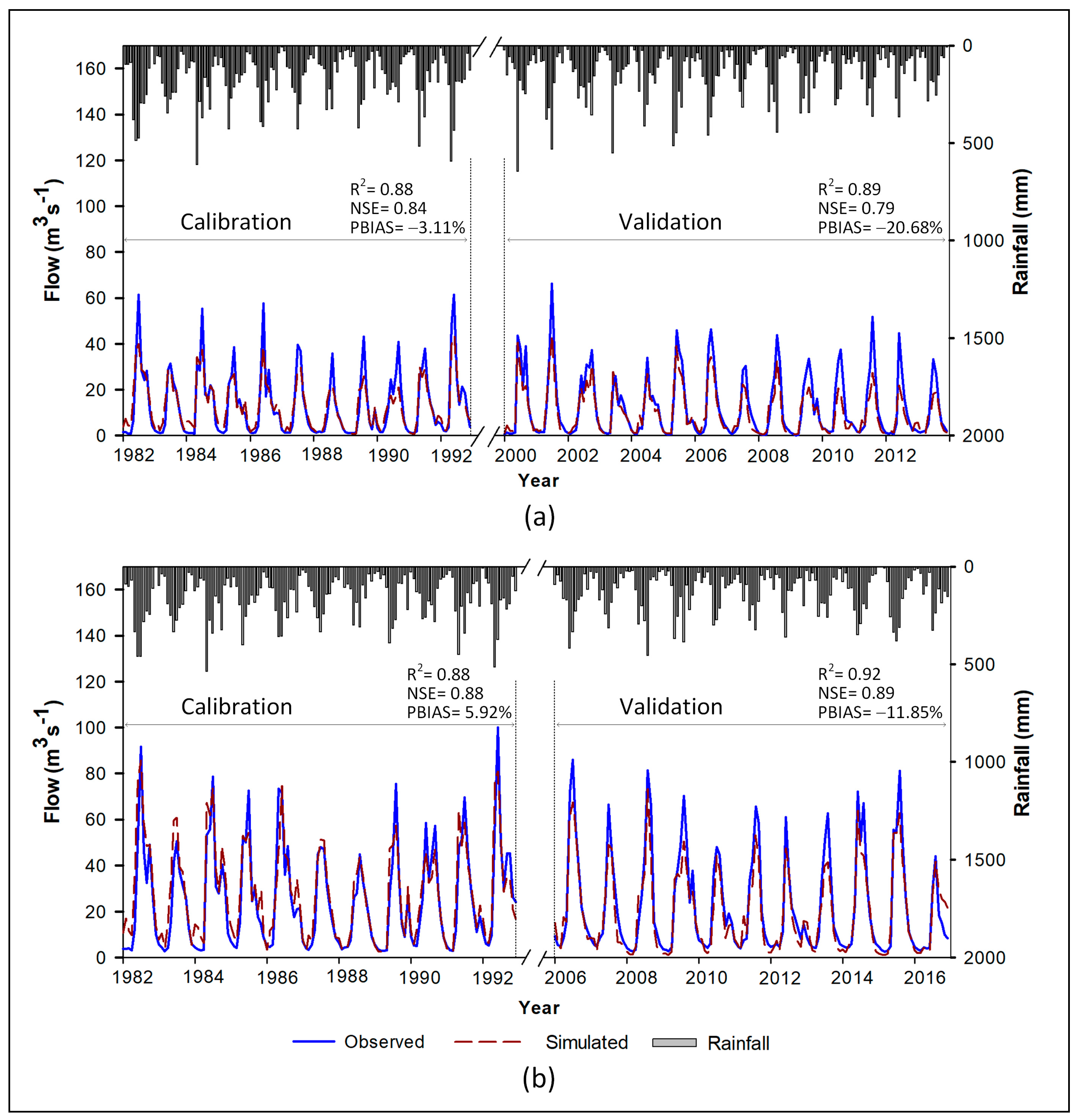
3.1. Model Calibration and Validation

According to the hydrological network, Quino and Muco basins were divided into 99 and 91 sub-basins with average surfaces of 3.02 km2 and 7.16 km2, respectively. In this way, the surface range of the sub-basins oscillates between 0.006 km2 and 14.33 km2 in Quino and between 0.01 km2 and 45.93 km2 in the Muco basin. The SWAT model was run to obtain the water discharge in all the sub-basins for both watersheds.
The model performance was calculated in the lowest basin points corresponding to the fluviometric stations Rio Quino en Longitudinal and Rio Muco en Puente Muco (Figure 2). In the Quino basin, the determination coefficient and the Nash–Sutcliffe efficiency parameter presented performance classification of “very good”, showing R2 values of 0.88 and 0.89 and NSE 0.84 and 0.79 in the calibration and validation, respectively, on a monthly scale. The percentage of bias in the calibration maintained a “very good” index (−3.11%), and the statistic obtained in the validation (−20.68) was classified as satisfactory by Moriasi et al. [38] (Figure 3a). On the other hand, in the Muco basin, statistics obtained showed “very good” classification for R2 (0.88 and 0.92) and NSE (0.88 and 0.89) in the calibration and validation process, respectively. The PBIAS showed a “very good” performance in the calibration phase (5.92%) and “good” in the validation phase (−11.85%) (Figure 3b).
Figure 3 depicts the performance of the discharge simulations during the calibration and validation periods for both basins. Performance values recorded “very good” to “satisfactory” grades, according to the classification proposed by Moriasi et al. [38], considering monthly scale verification.

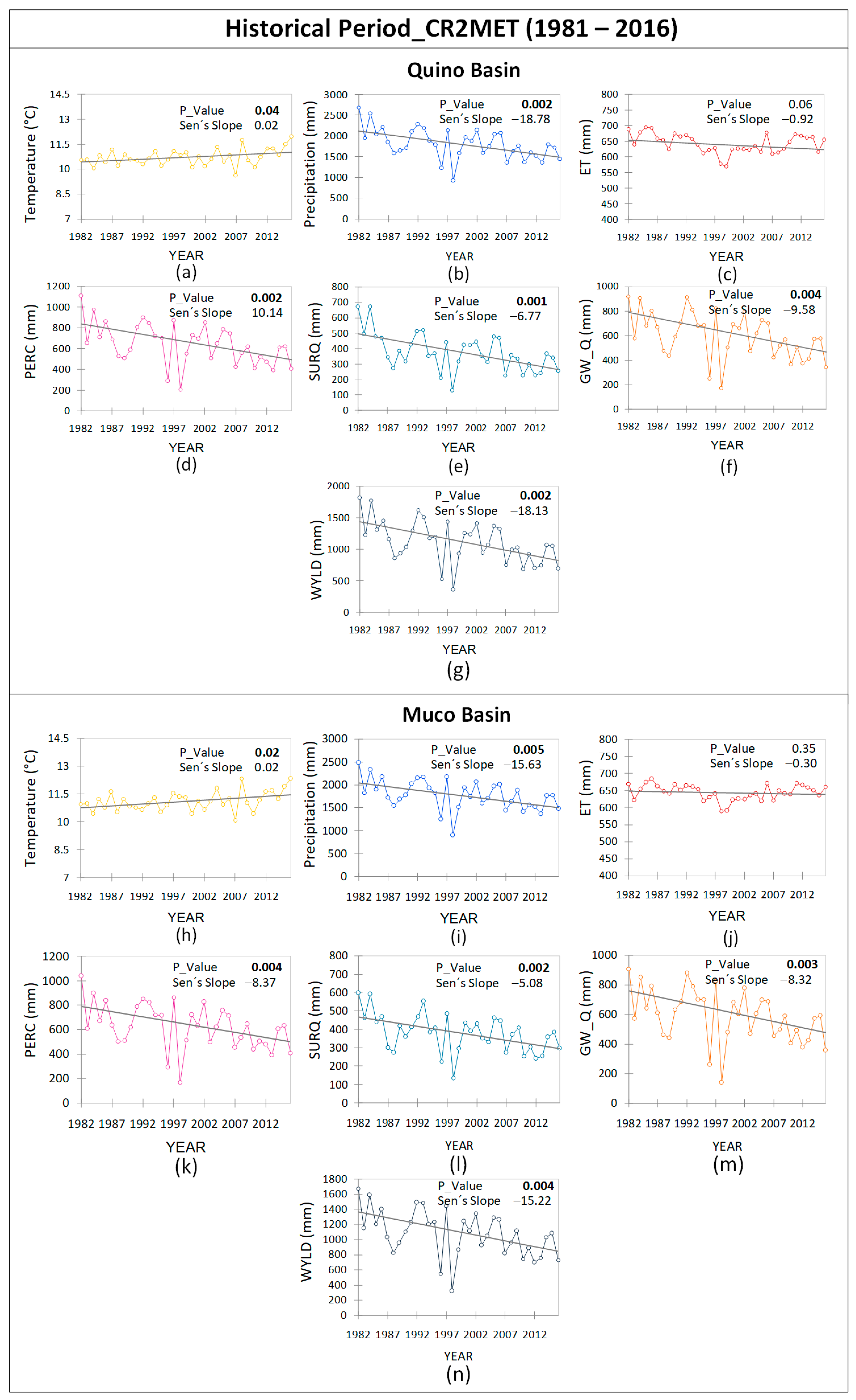
3.2. Annual Variation of the Hydrometeorological Components in the Last 35 Years

According to the results reported in Figure 4, the yearly variation trend of the hydrological components is directly related to the meteorological parameters (Figure 4). In order to evaluate such changes in the climate and hydrology of the study basins, 35 years of data within the period from 1982–2016 were analyzed. The average annual temperature for the period was 10.7 °C and 11.1 °C for Quino and Muco basin, respectively (Figure 4a,h), while the Mann–Kendall test showed a significant increasing trend, with p-values of 0.04 and 0.02, respectively.
The precipitation in the study basins presented a significant decreasing trend during the period, with p-value of 0.002 (Quino) and 0.005 (Muco) (Figure 4b,i). The mean annual precipitation value of the period for the Quino basin was 1811 mm, while for the Muco basin it was 1781 mm. Such a decreasing trend in precipitation, in addition to the temperature increase during these years, could cause a decrease in hydrological components such as ET, PERC, SURQ, GW_Q and WYLD, as shown in the model results.
Additionally, during the 35-year period, the evapotranspiration presented an annual average of 643 mm for Quino and values around 646 mm for Muco basin (Figure 4c,j). This parameter does not show a significant trend in its behavior; however, the remaining hydrological components presented significant trends according to the Mann–Kendall test. Yearly mean values obtained for PERC, SURQ, GW_Q and WYLD were 644 mm, 377 mm, 599 mm and 1111 mm, respectively, for Quino basin (Figure 4d–g). Meanwhile, for Muco basin the annual averages for the period were 626 mm (PERC), 378 mm (SURQ), 590 mm (GW_Q) and 1081 mm (WYLD) (Figure 4k–n), showing similar behavior in both basins.

3.3. Climate Change Effect on the Hydrological Cycle Components

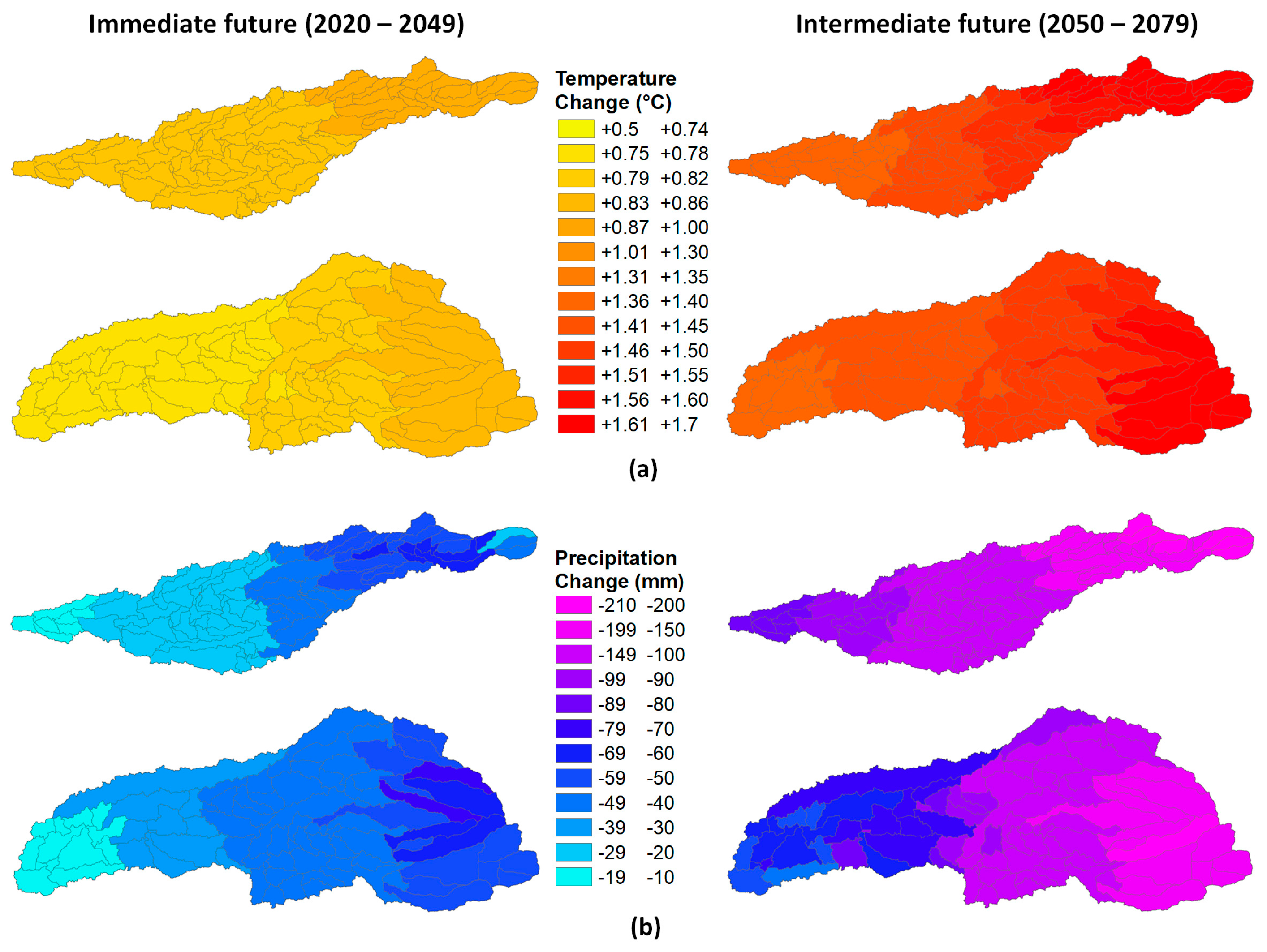
3.3.1. Input Parameters: Temperature and Precipitation

Figure 5 depicts expected changes in temperatures and rainfall for the Quino and Muco basins as calculated by using the local climate model RegCM4-MPI-ESM-MR, under the climate scenario RCP8.5. Considerable differences can be observed between the immediate and intermediate future periods. In this way, according to the Student’s t test, temperature increased significantly for both basins for each of the projected climatic periods (Figure 5a). A significant and increased temperature rise can be observed as spatially represented from downstream to upper stream both in the Quino and Muco basins. Furthermore, predicted precipitation changes (Figure 5b) indicate a significant decrease for both study areas with a p-value <0.0001 for immediate and intermediate future climatic periods. As shown, the higher changes in precipitation for both basins are expected to occur upstream. Raw p-values of the tests for input data and water cycle parameters modeled are reported as information in Appendix A, Table A1.
The aforementioned increase in temperature and a decrease in precipitation could be even expected for both climatic periods. The greatest changes are predicted to occur in the intermediate future, with an increase up to 1.7 °C in the mean yearly temperature and an average yearly precipitation decrease up to 200 mm (Figure 5a,b). Such trends agree with the behavior observed during the historical period.

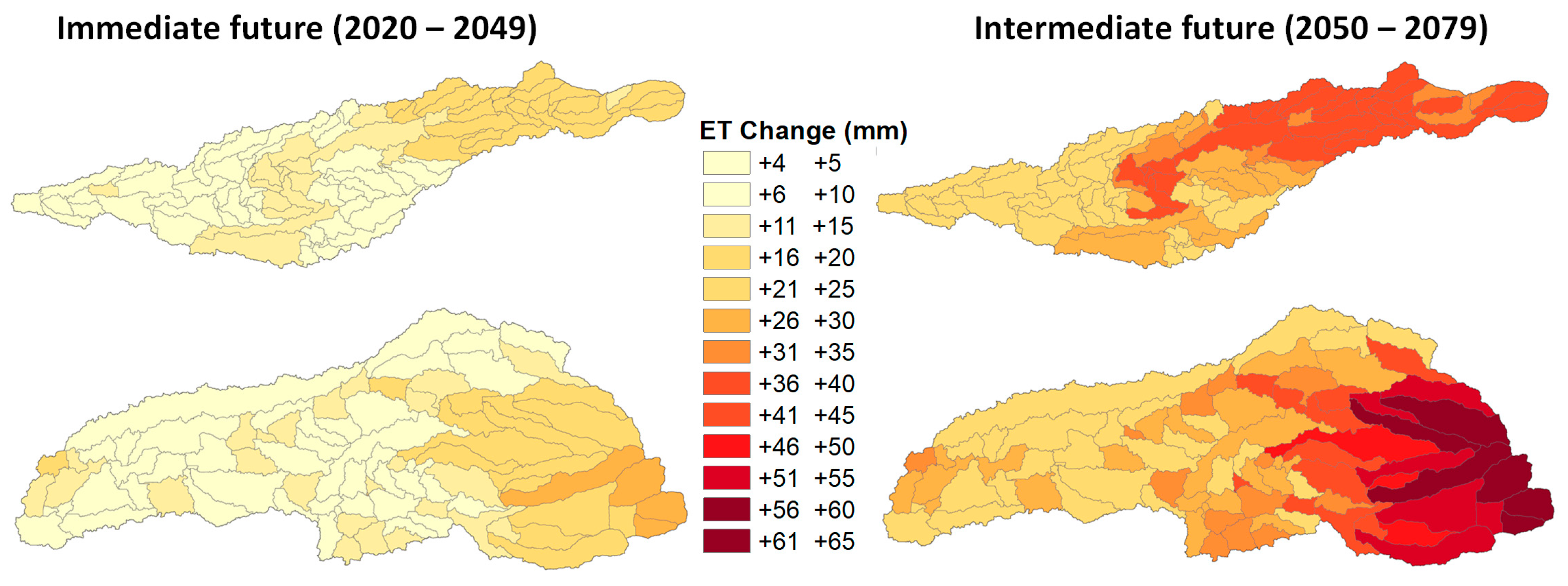
3.3.2. Evapotranspiration (ET)

The geographic distribution of the projected changes in evapotranspiration is represented in Figure 6. According to the Student’s t test, for both periods significant differences exist with p-values <0.0001 for both basins. The higher increase in evapotranspiration is expected to occur in the mountain area of both basins.
Yearly evapotranspiration change averages in the immediate future show maximum projected values of 25 mm and 30 mm for Quino and Muco basins, respectively. Changes projected for the intermediate future almost double the immediate scenario with maximum values reaching 45 mm and 65 mm, respectively (Figure 6).

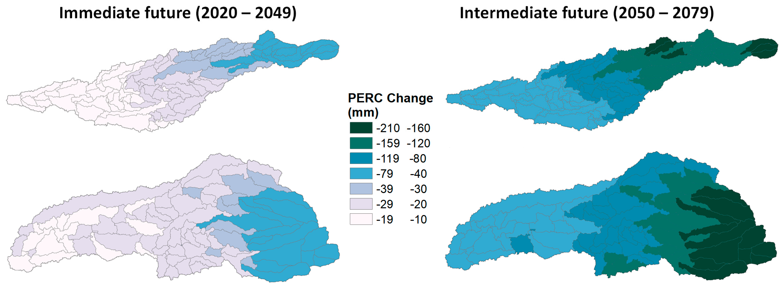
3.3.3. Percolation (PERC)

Similarly, percolation projections in the study basins depict significant decreasing trends during the climatic periods analyzed. Results represented in Figure 7 show the geographical spread of the decreasing trend in this water cycle parameter for both basins during the next decades, with the highest changes in the mountain area. For the immediate future, the model suggests the slightest changes in the lower and intermediate zone of both basins, with average yearly values ranging between 10 mm and 39 mm. The highest changes in percolation are expected to occur in the intermediate future with maximum average change of up to 210 mm in the yearly values for both study basins.
The decreasing trend is consistent in both river basins, indicating an intensification of the trend observed since the historical period analysis (Figure 7).

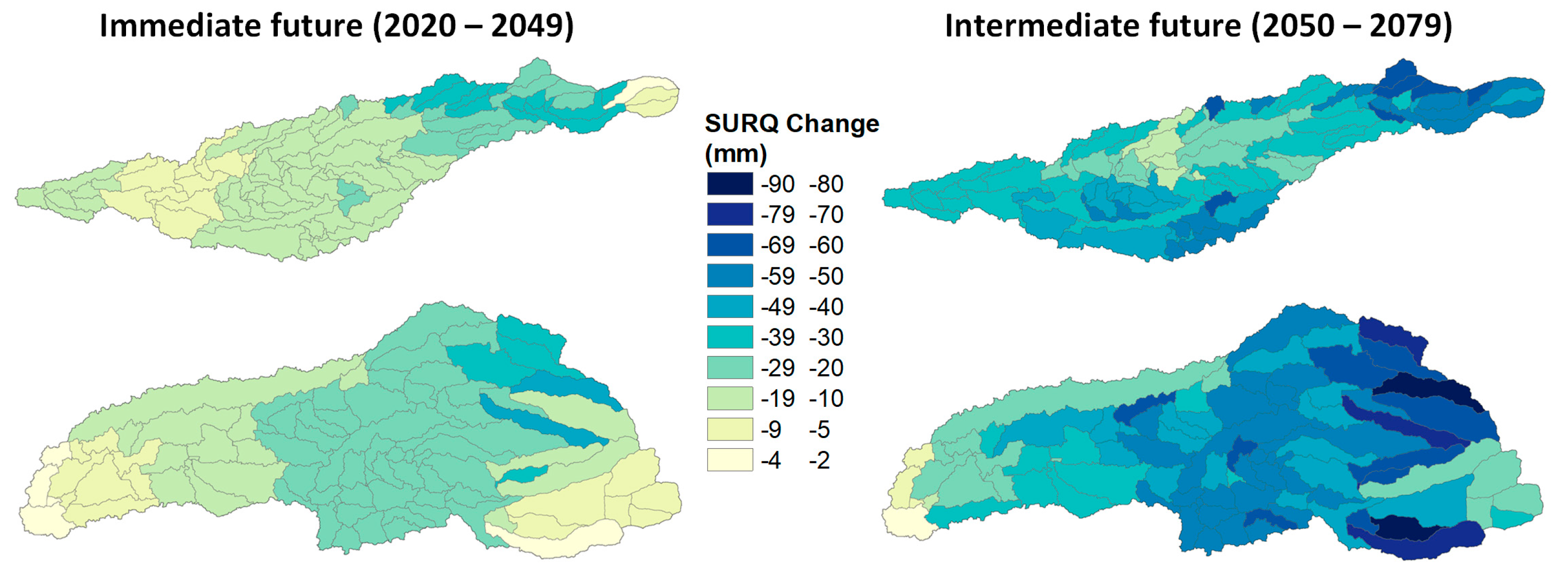
3.3.4. Surface Runoff (SURQ)

Following the performed analysis, the surface runoff shows a decreasing trend in both basins during the projected climatic periods, with a greater decrease in the intermediate future (Figure 8). According to Student’s t test, significant differences could be predicted with p-values lower than 0.0001. The variation of this water cycle parameter during the immediate future seems to be limited downstream, changing less than 10 mm. However it would be geographically balanced in the middle part of the basins where the largest number of sub-basins with projected annual variation reaching 59 mm can be found. However, in the intermediate future, the Quino basin does not present a clearly homogeneous correlation to height. Meanwhile, in the Muco basin, a marked decreasing variation is observed as the height increases in almost all its sub-basins.
For both climatic periods, the statistical tests highlight a generalized and significant decrease in the surface runoff; such a trend also agrees with the changes observed during the historical period.

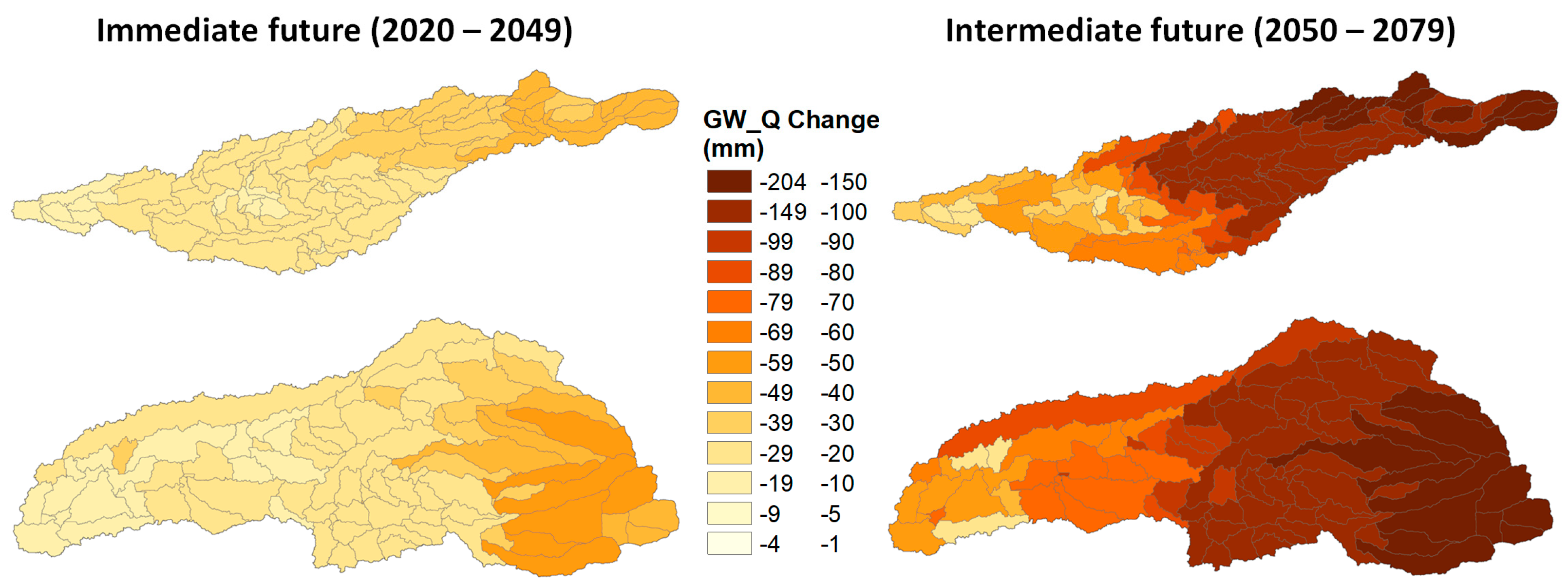
3.3.5. Groundwater Flow (GW_Q)

Decreasing trends could also be predicted during both periods studied, with significant values for Quino and Muco basins for the groundwater flow. If analyzed as spatially distributed, a generalized change strongly influenced by the sub-basins altitude can be observed in Figure 9.
The groundwater flow projection worsens in the intermediate future with maximum variation values obtained up to 204 mm. This downward trend seems to be consistent with the behavior that occurred during the historical period.

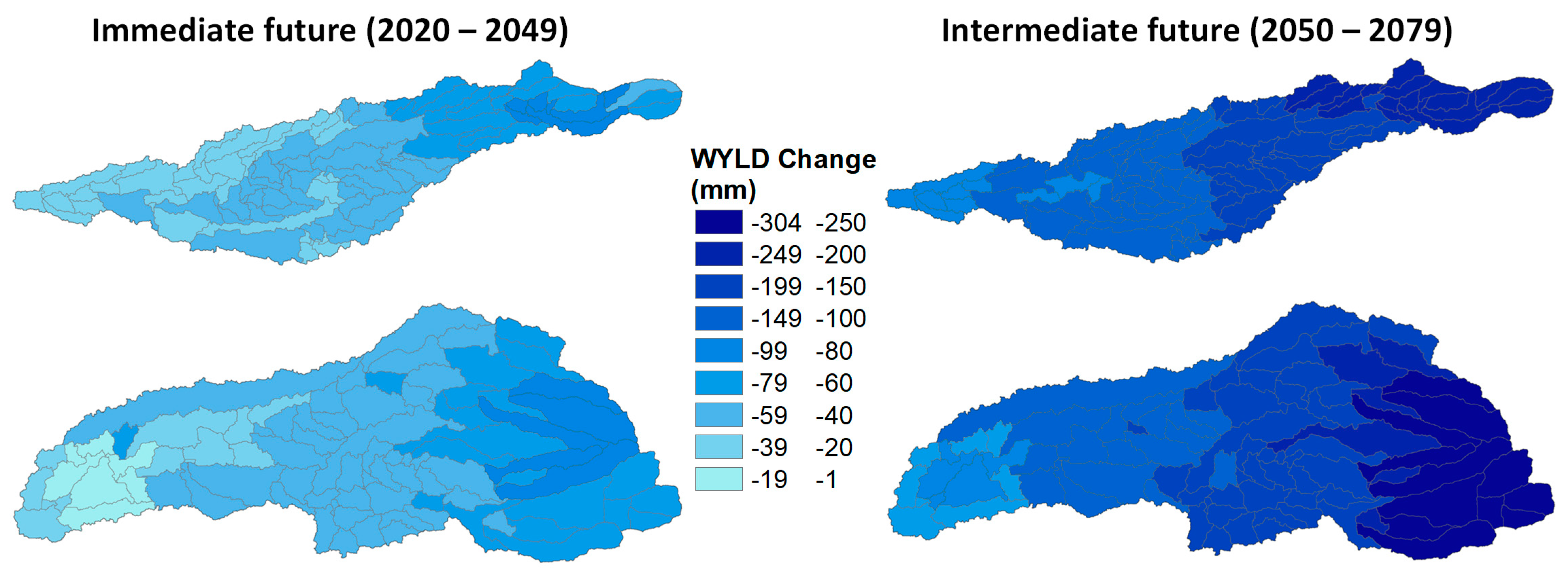
3.3.6. Water Yield (WYLD)

Finally, according to the Student’s t test, the projected water discharge suggests a significant decrease in the coming decades for both study basins (Figure 10) in all the sub-basins. It can be spatially distinguished that, as in the previous parameters, there is a marked relationship between the predicted changes and the sub-basin’s altitude, with a decrease in projected discharge greater as the elevation increases for both hydrographic basins.
It is worth noting that the trends obtained for both climatic periods seem homogeneous, showing a discharge decrease. However, this tendency seems to intensify during the intermediate future if compared to the immediate future (Figure 10).
The yearly average decrease in discharge for the intermediate future in the lower and middle areas of the basins could reach 80 mm to 200 mm, while in the mountainous area a drop of up to 304 mm could be expected. This significant reduction projected in the Quino and Muco basins for each of their sub-basins is also consistent with the trend obtained in the historical period (Figure 10).

3.3.7. Relative and Absolute Changes of the Hydrological Balance Components at a Basin Scale

Table 2 shows the yearly relative and absolute changes in Quino and Muco basins for both periods modeled at a basin scale. As it was expected from previous sections, higher average change percentage could be expected in almost every parameter for the intermediate future if compared to the immediate future.
In both climatic periods, temperature is the parameter with the highest relative change both for Quino and for Muco basin, projecting a maximum increase of 14.78% and 14.16%, respectively. Ordered from highest to lowest change are the PERC, GW_Q, ET and WYLD parameters, while the SURQ presented the lowest relative change with a decrease of 0.72% and 0.58% (immediate future and intermediate future) for Quino basin and 1.31% and 0.84% (immediate future and intermediate future) for Muco basin.

4. Discussion

It could be expected that, by incorporating the precipitation and temperature anomaly from a future climate scenario (RCP8.5), the remaining water cycle components become modified, since precipitation is the main component of change in the hydrological cycle and basically confers it mobility [51,52,53]. On the other hand, temperature is one of the components governing evapotranspiration [54], and the transpiration fraction is the process causing greatest water loss in the basin system [55]. This is why, when these drivers become altered, the components of the water balance are also modified.
These temperature and rainfall changes both in the Quino and Muco basins seems to be induced from moderate to severe changes in the regime of the hydrological cycle components evaluated. Obtained results imply that the average annual temperature increase up to 1.5 °C, representing a percentage change of 14.78% and 14.16% for Quino and Muco, respectively, leads to a decrease in PERC (−9.52 mm and −9.73 mm), SURQ (−2.38 mm and −1.76 mm), GW_Q (−7.44 mm and –8.14 mm) and WYLD (−5.25 mm and −4.98 mm) and an increase in ET (+5.26 mm and +5.81 mm) for Quino and Muco basins, respectively, in the intermediate future scenario. The potential loss of water resources through the deficit of rainfall and greater evaporation has been quantified in different studies, reaffirming that this geographical area of Chile is particularly vulnerable to climate change [16,56,57,58,59].
On the other hand, in both study basins, on a spatial scale, it can be observed that the annual average changes for both study periods (immediate future and intermediate future) present the same behavioral trend following a staggered pattern. It is relevant that the greatest changes in ET, PERC, SURQ, GW_Q and WYLD take place in the mountainous zone (pre-mountain range) and minor changes in the alluvial plain (central depression). The behavior of these parameters is directly related to the temperature increase behavior between 0.5 °C and 1.7 °C from the lower part to the upper part of the basin, respectively, and a decrease in precipitation of 10 mm to 200 mm between the two time periods for these geographical areas.
A similar behavior, different in geographical area, was also reported by Falvey and Garreaud [60]. They observed a cooling of coastal temperatures and a gradual warming over the Andes mountain range for the central and northern zone of Chile. They reported a decrease in temperatures (−0.15°/decade) along the coast, slight increases both in the central valley and the mountain range stations, with a significant increase of almost +0.25 °C per decade. The orographic effect induced by the Andes Mountains on precipitation defines a remarkable character of the hydrological regime in the central-southern region of the country, where precipitation on the slopes of the mountains can be from two to three times greater than in the lower elevations [59,61]. This effect, in addition to the climatic projections, could cause a greater change for the windward Andes slope.
Several studies suggest variable hydrological responses of the water cycle parameter as the effect of future climate change scenarios around the world. For instance, Chien et al. (2013) suggest an annual flow reduction around 41.1% and 45.2% for the period from 2051–2060 in a study including four basins of the mid-west zone of the United States. Qi et al. (2009) indicated that increasing 2.8 °C in temperature causes a change in real evapotranspiration and water production of +6.2% and −13.9%, respectively. Andreini et al. [62] concluded that the large changes that occur in surface runoff correspond to a lesser change in precipitation. Additionally, in India, Pandey et al. [63] quantified the climate change impact (2071–2100) in the Armur basin using SWAT, suggesting that evapotranspiration and water production will increase 28% and 49%, respectively.
Grusson et al. [19] also compared different climatic ensembles in the south zone of France during 2010–2050. In their study, a strong impact on green water was shown, specifically a reduction in soil water content (SWC) and a substantial increase in evapotranspiration (ET) in winter. In summer, however, the ET faced lower flows due to the lack of SWC, which highlights future deficits of green water reserves. Besides, Yu et al. [23] showed an increase in annual runoff depth at the northeast zone of China by 18.1% (RCP 2.6), 11.8% (RCP 4.5), 23.6% (RCP 6.0) and 11.5% (RCP8.5), compared to the base years. Therefore, worldwide, differentiated behavior can be observed depending on the physical–geographical conditions of each study area.
Specifically in Chile, Stehr et al. [24] modeled the hydrological response to climate change in two sub-basins of the Biobío River, depicting that a 30% decrease in precipitation could conduct a 45% and 32% reduction in the water flow of the study sub-basins. In addition, Barrientos et al. [64] recently reported an study also conducted in experimental sub-basins of the BioBio river obtaining similar results in the trends. Even when these forecasts suggest more dramatic reductions in precipitation and runoff than the present study, the observed trends become similar. Generally, as it has been reported by the (CR)2 group studies [33] and as the aforementioned studies suggest, the warming effects and consequences seem to be greater for northern than for southern zones in Chile [33].
Finally, the present study showed that future climate projections maintain the same behavioral trend that was evidenced in the simulated past. This similarity shows the quality of the data used for the study and the correct performance of the calibration and validation for both study basins (Quino and Muco). In this way, it can be stated that the performance metrics calculated after the configuration of the SWAT model by the calibration and validation procedures are functional for long-term hydro-climatic evaluation in the south-central zone of Chile.
However, as temperatures rise and precipitation decreases, the land cover/use is unlikely to remain unchanged until 2079 even without human intervention. It is necessary to develop studies addressing the individual and combined effects of the land use/cover change and future climate change in basins of the south-central zone of Chile. The importance of treating the data in this way is to determine which of the alterations can affect the hydrological components to a greater and lesser extent in order to determine their individual and combined effect. This could help on the one hand understanding the effect of these two stressors on the components of the hydrological cycle and, on the other hand, to address most probable future scenarios. The present manuscript provides the first results to determine the importance of the individual effect of climate change in the south-central zone of Chile. Future work by this group will intend to study the problems described above.

5. Conclusions

This study determined the possible effects of future climate on the water balance of the Quino and Muco basins for land use/cover by using the SWAT hydrological model. The hydrological response of the basin was simulated using the local climate model RegCM4-MPI-ESM-MR, for the future climate projection RCP8.5, as it is the most critical scenario in CMIP5. The future projection was divided into two time periods (immediate future and intermediate future). Calibration and sensitivity analyses were carried out to ensure that the hydrological model output was reliable. The results show for both analysis periods an increase in temperature and a decrease in precipitation. The analyzed parameters show the same trend behavior for both time periods; however, a greater impact in the intermediate future could be expected.
For the intermediate future, on an annual average, temperatures are expected to increase up to 1.7 °C and rainfall will decrease by around 210 mm. As a consequence, as temperature rises, ET would increase causing, combined with the precipitation effect, a decrease in PERC, SURQ, GW_Q and WYLD. Additionally, the study results suggest that the expected changes for both periods of time would present the same behavior that has occurred since the 1980s, with a greater effect on the intermediate future.
The present investigation results could be useful for future studies in areas such as native forest cover, forest plantation and agriculture. Furthermore, information is provided to investigate how future climate changes could affect hydrological processes in watersheds located in the central south zone of Chile. The data and results shown here could help in the integrated and sustainable basin management within the region.

Author Contributions

Conceptualization, R.M.-R., M.A., and A.S.; methodology, R.M.-R., M.A., N.J.A. and A.S.; software, R.M.-R., M.A., S.S., and J.-M.S.-P.; validation, R.M.-R., M.A., N.J.A., A.S., S.S., and J.-M.S.-P.; formal analysis, R.M.-R.,M.A., N.J.A., A.S., I.D.-L., L.R.-L., S.S., and J.-M.S.-P.; investigation, R.M.-R., M.A., and A.S.; resources, R.M.-R., M.A., and A.S.; data curation, R.M.-R., writing—original draft preparation, R.M.-R., M.A., and N.J.A., writing—review and editing, R.M.-R., M.A., N.J.A., A.S., I.D.-L., L.R.-L., S.S., and J.-M.S.-P.; visualization, R.M.-R., N.J.A., I.D.-L.; supervision, M.A., A.S., S.S., and J.-M.S.-P.; project administration, R.M.-R. and M.A.; funding acquisition, R.M.-R. and M.A. All authors have read and agreed to the published version of the manuscript.

Funding

This research was funded by ANID, PCHA/Doctorate National 2016 (Grant N_ 21160323) and project VRID-Enlace N_ 218.191.002-1.

Institutional Review Board Statement

Not applicable.

Informed Consent Statement

Not applicable.

Data Availability Statement

Data is contained within the article.

Acknowledgments

We appreciate ANID, PCHA/Doctorate National 2016 (Grant N_ 21160323) and project VRID-Enlace N_ 218.191.002-1 for the financial founding provided. Authors thank the support provided by the University of Concepcion and ECOLAB laboratory UMR 5262. Authors especially thank the Center for Climate and Resilience Research (CR)2 for providing the meteorological data.

Conflicts of Interest

The authors declare no conflict of interest.

Appendix A

Table A1. Raw p_values for t-student mean comparison test: Climatic scenarios pairs.
Average Values Comparison. Climatic Model RegCM4-MPI-ESM-MR; Projection RCP8.5
Hydrological ParametersQuino Basin
Historical Period/Inmediate FutureHistorical Period/Intermediate FutureInmediate Future/Intermediate Future
Precipitation2.22162 × 10−442.22507 × 10−589.42665 × 10−62
Temperature3.166 × 10−1541.2993 × 10−1283.793 × 10−110
ET1.0493 × 10−441.47193 × 10−562.23042 × 10−59
PERC1.12169 × 10−408.92672 × 10−421.97279 × 10−41
SURQ6.1165 × 10−347.69659 × 10−539.02548 × 10⁻³³
GW_Q2.78038 × 10−521.84815 × 10−375.75124 × 10⁻³²
WYLD7.16781 × 10−526.69911 × 10−553.25865 × 10−53
Hydrological ParametersMuco Basin
Historical Period/Inmediate FutureHistorical Period/Intermediate FutureInmediate Future/Intermediate Future
Precipitation1.17591 × 10−102.24552 × 10−326.56955 × 10−40
Temperature4.73665 × 10−862.8399 × 10−1001.08209 × 10−98
ET6.70625 × 10−283.30886 × 10−423.51845 × 10−51
PERC2.21472 × 10−215.97748 × 10−425.8181 × 10−46
SURQ1.77134 × 10−067.06603 × 10−198.57832 × 10⁻³⁵
GW_Q3.90917 × 10−181.20551 × 10−401.14199 × 10−47
WYLD2.6065 × 10−125.32872 × 10−346.41939 × 10−43

References

  1. UNEP GEO 5. Perspectivas del Medio Ambiente Mundial: Medio Ambiente Para el Futuro que Queremos; UNEP: Nairobi, Kenya, 2012. [Google Scholar]
  2. UNEP GEO-6. Regional Assessment for Latin America and the Caribbean; UNEP: Nairobi, Kenya, 2016. [Google Scholar]
  3. Kundzewicz, Z.; Mata, L.; Arnell, N.; Döll, P.; Kabat, P.; Jiménez, B.; Miller, K.; Oki, T.; Sen, Z.; Shiklomanov, I. Freshwater resources and their management. Climate Change 2007: Impacts, Adaptation and Vulnerability. In Current Opinion in Environmental Sustainability; Contribution of Working Group II to the Fourth Assessment Report of the Intergovernmental Panel on Climate Change; Parry, M.L., Canziani, O.F., Palutikof, J.P., van der Linden, P.J., Hanson, C.E., Eds.; Cambridge University Press: Cambridge, UK, 2007; pp. 173–210. [Google Scholar]
  4. IPCC. Climate Change 2014: Impacts, Adaptation, and Vulnerability. Part B: Regional Aspects. In I to the Fifth Assessment Report of the Intergovernmental Panel on Climate Change; Barros, V.R., Field, C.B., Dokken, D.J., Mastrandrea, M.D., Mach, K.J., Bilir, T.E., Chatterjee, M., Ebi, K.L., Estrada, Y.O., Genova, R.C., et al., Eds.; Cambridge University Press: Cambridge, UK; New York, NY, USA, 2014; pp. 1133–1197. [Google Scholar]
  5. Arnell, N.W.; Reynard, N.S. The effects of climate change due to global warming on river flows in Great Britain. J. Hydrol. 1996, 183, 397–424. [Google Scholar] [CrossRef]
  6. Lambin, E.F.; Turner, B.L.; Geist, H.J.; Agbola, S.B.; Angelsen, A.; Bruce, J.W.; Coomes, O.T.; Dirzo, R.; Fischer, G.; Folke, C.; et al. The causes of land-use and land-cover change: Moving beyond the myths. Glob. Environ. Chang. 2001, 11, 261–269. [Google Scholar] [CrossRef]
  7. Akoko, G.; Kato, T.; Tu, L.H. Evaluation of irrigation water resources availability and climate change impacts-a case study of Mwea irrigation scheme, Kenya. Water 2020, 12, 2330. [Google Scholar] [CrossRef]
  8. Núñez-Hidalgo, I. Climate Change: Impacts, Policy and Perspectives. In Chile. Environmental History, Perspectives and Challenges; Alberto, J., Ed.; Alaniz: Santiago, Chile, 2019; pp. 119–154. ISBN 9781536156652. [Google Scholar]
  9. Sarricolea, P.; Herrera-Ossandon, M.; Meseguer-Ruiz, Ó. Climatic regionalisation of continental Chile. J. Maps 2017, 13, 66–73. [Google Scholar] [CrossRef]
  10. Gutiérrez, D.; Akester, M.; Naranjo, L. Productivity and sustainable management of the Humboldt current large marine ecosystem under climate change. Environ. Dev. 2016, 17, 126–144. [Google Scholar] [CrossRef]
  11. Araya-Osses, D.; Casanueva, A.; Román-Figueroa, C.; Uribe, J.M.; Paneque, M. Climate change projections of temperature and precipitation in Chile based on statistical downscaling. Clim. Dyn. 2020, 54, 4309–4330. [Google Scholar] [CrossRef]
  12. CONAMA-DGF. Estudio de la Variabilidad Climática en Chile Para el Siglo XXI; CONAMA: Santiago, Chile, 2006. [Google Scholar]
  13. Garreaud, R. Cambio Climático: Bases Físicas e Impactos en Chile. Rev. Tierra Adentro-INIA 2011, 14. Available online: http://www.dgf.uchile.cl/rene/PUBS/inia_RGS_final.pdf (accessed on 15 December 2020).
  14. Orrego, R.; Abarca-del-Río, R.; Ávila, A.; Morales, L. Enhanced mesoscale climate projections in TAR and AR5 IPCC scenarios: A case study in a Mediterranean climate (Araucanía Region, south central Chile). Springerplus 2016, 5, 1669. [Google Scholar] [CrossRef] [Green Version]
  15. Prudhomme, C.; Giuntoli, I.; Robinson, E.L.; Clark, D.B.; Arnell, N.W.; Dankers, R.; Fekete, B.M.; Franssen, W.; Gerten, D.; Gosling, S.N.; et al. Hydrological droughts in the 21st century, hotspots and uncertainties from a global multimodel ensemble experiment. Proc. Natl. Acad. Sci. USA 2014, 111, 3262–3267. [Google Scholar] [CrossRef] [Green Version]
  16. Pinto, F. Cambio climático en Chile: Del desafío global a la oportunidad local. Friedich Ebert Stift. 2019. Available online: https://library.fes.de/pdf-files/bueros/chile/15512.pdf (accessed on 20 November 2020).
  17. McNamara, I.; Nauditt, A.; Zambrano-Bigiarini, M.; Ribbe, L.; Hann, H. Modelling water resources for planning irrigation development in drought-prone southern Chile. Int. J. Water Resour. Dev. 2020, 1–26. [Google Scholar] [CrossRef]
  18. Hao, Y.; Ma, J.; Chen, J.; Wang, D.; Wang, Y.; Xu, H. Assessment of changes in water balance components under 1.5 °C and 2.0 °C global warming in transitional climate basin by multi-RCPs and multi-GCMs approach. Water 2018, 10, 1863. [Google Scholar] [CrossRef] [Green Version]
  19. Grusson, Y.; Anctil, F.; Sauvage, S.; Sánchez Pérez, J.M. Coevolution of hydrological cycle components under climate change: The case of the Garonne River in France. Water 2018, 10, 1870. [Google Scholar] [CrossRef] [Green Version]
  20. Makhtoumi, Y.; Li, S.; Ibeanusi, V.; Chen, G. Evaluating water balance variables under land use and climate projections in the upper choctawhatchee River Watershed, in Southeast US. Water 2020, 12, 2205. [Google Scholar] [CrossRef]
  21. Abbaspour, K.C.; Vaghefi, S.A.; Srinivasan, R. A guideline for successful calibration and uncertainty analysis for soil and water assessment: A review of papers from the 2016 international SWAT conference. Water 2017, 10, 6. [Google Scholar] [CrossRef] [Green Version]
  22. Ficklin, D.L.; Luo, Y.; Luedeling, E.; Gatzke, S.E.; Zhang, M. Sensitivity of agricultural runoff loads to rising levels of CO2 and climate change in the San Joaquin Valley watershed of California. Environ. Pollut. 2010, 158, 223–234. [Google Scholar] [CrossRef]
  23. Yu, Z.; Man, X.; Duan, L.; Cai, T. Assessments of impacts of climate and forest change on water resources using swat model in a subboreal watershed in northern da hinggan mountains. Water 2020, 12, 1565. [Google Scholar] [CrossRef]
  24. Stehr, A.; Debels, P.; Arumi, J.L.; Alcayaga, H.; Romero, F. Modelación de la respuesta hidrológica al cambio climático: Experiencias de dos cuencas de la zona centro-sur de Chile. Tecnol. Cienc. Agua 2010, 1, 37–58. [Google Scholar]
  25. Olson, D.M.; Dinerstein, E. The global 200: Priority ecoregions for global conservation. Ann. Missouri Bot. Gard. 2002, 89, 199–224. [Google Scholar] [CrossRef]
  26. Myers, N. Biodiversity Hotspots Revisited. Bioscience 2003, 53, 916–917. [Google Scholar]
  27. Neitsch, S.L.; Arnold, J.G.; Kiniry, J.R.; Williams, J.R. Soil and Water Assessment Tool. Theoretical Documentation; Soil and Water Research Laboratory: Temple, TX, USA, 2005. [Google Scholar]
  28. Arnold, J.G.; Kiniry, J.R.; Srinivasan, R.; Williams, J.R.; Haney, E.B.; Neitsch, S.L. SWAT 2012 Input/Output Documentation; Texas Water Resources Institute: College Station, TX, USA, 2012; p. 30. [Google Scholar]
  29. Hargreaves, G.H.; Samani, Z.A. Samani Reference Crop Evapotranspiration from Temperature. Appl. Eng. Agric. 1985, 1, 96–99. [Google Scholar] [CrossRef]
  30. CIREN Estudio Agrologico IX Región. Descripciones de Suelos: Materiales y Símbolos. (Pub. CIREN N°122); Publicaciones CIREN: Santiago, Chile, 2002; ISBN 956-7153-35-3. [Google Scholar]
  31. Heilmayr, R.; Echeverría, C.; Fuentes, R.; Lambin, E.F. A plantation-dominated forest transition in Chile. Appl. Geogr. 2016, 75, 71–82. [Google Scholar] [CrossRef] [Green Version]
  32. Centro de Ciencia del Clima y la Resiliencia (CR)2. Guía Para la Plataforma de Visualizacion de Simulaciones Climáticas; (CR)²: Santiago, Chile, 2018; Volume 36. [Google Scholar]
  33. Centro de Ciencia del Clima y la Resiliencia (CR)2. Simulaciones Climáticas Regionales. 2018, Volume 26. Available online: http://www.cr2.cl/wp-content/uploads/2019/06/Simulaciones-clima%CC%81ticas-regionales-2018.pdf (accessed on 20 November 2020).
  34. Javaherian, M.; Ebrahimi, H.; Aminnejad, B. Prediction of changes in climatic parameters using CanESM2 model based on Rcp scenarios (case study): Lar dam basin. Ain Shams Eng. J. 2021, 12, 445–454. [Google Scholar] [CrossRef]
  35. Abbaspour, K.C.; Yang, J.; Maximov, I.; Siber, R.; Bogner, K.; Mieleitner, J.; Zobrist, J. Modelling hydrology and water quality in the pre-alpine/alpine Thur watershed using SWAT. J. Hydrol. 2007, 333, 413–430. [Google Scholar] [CrossRef]
  36. Martínez-Retureta, R.; Aguayo, M.; Stehr, A.; Sauvage, S.; Echeverría, C.; Sánchez-Pérez, J.M. Effect of land use/cover change on the hydrological response of a southern center basin of Chile. Water 2020, 12, 302. [Google Scholar] [CrossRef] [Green Version]
  37. Abbaspour, K.C.; Rouholahnejad, E.; Vaghefi, S.; Srinivasan, R.; Yang, H.; Kløve, B. A continental-scale hydrology and water quality model for Europe: Calibration and uncertainty of a high-resolution large-scale SWAT model. J. Hydrol. 2015, 524, 733–752. [Google Scholar] [CrossRef] [Green Version]
  38. Moriasi, D.N.; Arnold, J.G.; Van Liew, M.W.; Bingner, R.L.; Harmel, R.D.; Veith, T.L. Model Evaluation Guidelines for Systematic Quantification of Accuracy in Watershed Simulations. Trans. ASABE 2007, 50, 885–900. [Google Scholar] [CrossRef]
  39. Rostamian, R.; Jaleh, A.; Afyuni, M.; Mousavi, S.F.; Heidarpour, M.; Jalalian, A.; Abbaspour, K.C. Application of a SWAT model for estimating runoff and sediment in two mountainous basins in central Iran. Hydrol. Sci. J. 2008, 53, 977–988. [Google Scholar] [CrossRef]
  40. Mann, H.B. Non-Parametric Test Against Trend. Econometrica 1945, 13, 245–259. [Google Scholar] [CrossRef]
  41. Kendall, M.G. Rank Correlation Methods; Griffin, C., Ed.; APA PsycInfo: London, UK, 1948. [Google Scholar]
  42. Gilbert, R. Statistical Methods for Environmental Pollution Monitoring; Van Nostrand Reinhold Co: New York, NY, USA, 1987; ISBN 0442230508. [Google Scholar]
  43. Onyutha, C.; Tabari, H.; Taye, M.T.; Nyandwaro, G.N.; Willems, P. Analyses of rainfall trends in the Nile River Basin. J. Hydro-Environ. Res. 2016, 13, 36–51. [Google Scholar] [CrossRef]
  44. Luo, K.; Tao, F.; Moiwo, J.P.; Xiao, D. Attribution of hydrological change in Heihe River Basin to climate and land use change in the past three decades. Sci. Rep. 2016, 6, 1–12. [Google Scholar] [CrossRef] [PubMed] [Green Version]
  45. Zeleňáková, M.; Purcz, P.; Poórová, Z.; Alkhalaf, I.; Hlavatá, H.; Portela, M. Monthly Trends of Precipitation in Gauging Stations in Slovakia. Procedia Eng. 2016, 162, 106–111. [Google Scholar] [CrossRef]
  46. Bari, S.H.; Rahman, M.T.U.; Hoque, M.A.; Hussain, M.M. Analysis of seasonal and annual rainfall trends in the northern region of Bangladesh. Atmos. Res. 2016, 176–177, 148–158. [Google Scholar] [CrossRef]
  47. Sen, P. Estimates of the Regression Coefficient Based on Kendall’s Tau. J. Am. Stat. Assoc. 1968, 63, 1379–1389. [Google Scholar] [CrossRef]
  48. Theil, H. A Rank-Invariant Method of Linear and Polynomial Regression Analysis; Springer: Dordrecht, The Netherlands, 1992. [Google Scholar]
  49. Theil, H. A rank-invariant method of linear and polynomial regression analysis I, II, III I, II, III. Indag. Math. 1950, 12, 85. [Google Scholar]
  50. Gassman, P.W.; Reyes, M.R.; Green, C.H.; Arnold, J.G. The soil and water assessment tool: Historical development, applications, and future research directions. Trans. ASABE 2007, 50, 1211–1250. [Google Scholar] [CrossRef] [Green Version]
  51. Brutsaert, W. Hydrology: An Introduction; Cambridge University Press: Cambridge, UK, 2005. [Google Scholar]
  52. Davie, T. Fundamentals of Hydrology; Taylor y Francis: Oxfordshire, UK, 2008. [Google Scholar]
  53. Han, D. 2010 Concise Hydrology; Bookboon: London, UK, 2010; ISBN 9788776815363. [Google Scholar]
  54. Fitts, C. Groundwater Science, 2nd ed.; Academic Press: Cambridge, MA, USA, 2012; ISBN 0-12-257855-4. [Google Scholar]
  55. Fetter, C. Applied Hydrogeology, 4th ed.; Prentice Hall: Upper Saddle River, NJ, USA, 2000; ISBN 9780130882394. [Google Scholar]
  56. Vicuña, S.; McPhee, J.; Garreaud, R.D. Agriculture Vulnerability to Climate Change in a Snowmelt-Driven Basin in Semiarid Chile. J. Water Resour. Plan. Manag. 2012, 138, 431–441. [Google Scholar] [CrossRef]
  57. Demaria, E.M.C.; Maurer, E.P.; Thrasher, B.; Vicuña, S.; Meza, F.J. Climate change impacts on an alpine watershed in Chile: Do new model projections change the story? J. Hydrol. 2013, 502, 128–138. [Google Scholar] [CrossRef]
  58. Garreaud, R.; Alvarez-Garreton, C.; Barichivich, J.; Boisier, J.P.; Christie, D.; Galleguillos, M.; LeQuesne, C.; McPhee, J.; Zambrano-Bigiarini, M. The 2010–2015 mega drought in Central Chile: Impacts on regional hydroclimate and vegetation. Hydrol. Earth Syst. Sci. Discuss. 2017, 21, 6307–6327. [Google Scholar] [CrossRef] [Green Version]
  59. Boisier, J.P.; Alvarez-Garreton, C.; Cordero, R.R.; Damiani, A.; Gallardo, L.; Garreaud, R.D.; Lambert, F.; Ramallo, C.; Rojas, M.; Rondanelli, R. Anthropogenic drying in central-southern Chile evidenced by long-term observations and climate model simulations. Elementa 2018, 6, 74. [Google Scholar] [CrossRef]
  60. Falvey, M.; Garreaud, R.D. Regional cooling in a warming world: Recent temperature trends in the southeast Pacific and along the west coast of subtropical South America (1979–2006). J. Geophys. Res. Atmos. 2009, 114, 1–16. [Google Scholar] [CrossRef]
  61. Viale, M.; Garreaud, R. Orographic effects of the subtropical and extratropical Andes on upwind precipitating clouds. J. Geophys. Res. Atmos. 2015, 120, 4962–4974. [Google Scholar] [CrossRef]
  62. Andreini, M.; Giesen, N.; Edig, A.; Fosu, M.; Andah, W. Volta Water Balance; University of Bonn, Center for Development Research (ZEF): Bonn, Germany, 2000. [Google Scholar]
  63. Pandey, B.K.; Gosain, A.K.; Paul, G.; Khare, D. Climate change impact assessment on hydrology of a small watershed using semi-distributed model. Appl. Water Sci. 2017, 7, 2029–2041. [Google Scholar] [CrossRef] [Green Version]
  64. Barrientos, G.; Herrero, A.; Iroumé, A.; Mardones, O.; Batalla, R.J. Modelling the Effects of Changes in Forest Cover and Climate on Hydrology of Headwater Catchments in South-Central Chile. Water 2020, 12, 1828. [Google Scholar] [CrossRef]
Figure 1. Geographical location map of Quino and Muco basins. Gaugin Stations: (I) Rio Quino en Longitudinal and (II) Rio Muco en Puente Muco.
Water 13 00794 g001
Figure 2. Data used in SWAT to delimit the sub-basins, micro-basins and hydrological response units (HRU). (a) Land use, (b) soil type, (c) slope and (d) location of climatic information and fluviometric stations: (I) Rio Quino en Longitudinal and (II) Rio Muco en Puente Muco.
Water 13 00794 g002
Figure 3. Calibration and validation of the total monthly flow for (a) Quino basin and (b) Muco basin.
Water 13 00794 g003
Figure 4. Annual variability analysis for meteorological factors and hydrological components from 1976–2016 in Quino (left) and Muco (right) basins. Mann–Kendall test (MK) (significance level 0.05) and Sen’s slope (β > 0 increasing trend and β < 0 decreasing trend). Temperature, precipitation, evapotranspiration (ET), percolation (PERC), surface flow (SURQ), groundwater (GW_Q) and water yield (WYLD).
Water 13 00794 g004
Figure 5. Changes in the yearly average (a) temperature and (b) precipitation at the sub-basin scale, using RegCM4-MPI-ESM-MR, scenario RCP8.5. Upper basin: Quino, lower basin Muco.
Water 13 00794 g005
Figure 6. Changes in the yearly average evapotranspiration (ET) at the sub-basin scale, using RegCM4-MPI-ESM-MR, scenario RCP8.5.
Water 13 00794 g006
Figure 7. Changes in the yearly average percolation (PERC) at the sub-basin scale, using RegCM4-MPI-ESM-MR, scenario RCP8.5.
Water 13 00794 g007
Figure 8. Changes in the yearly average surface runoff (SURQ) at the sub-basin scale, using RegCM4-MPI-ESM-MR, scenario RCP8.5.
Water 13 00794 g008
Figure 9. Changes in the yearly average groundwater flow (GW_Q) at the sub-basin scale, using RegCM4-MPI-ESM-MR, scenario RCP8.5.
Water 13 00794 g009
Figure 10. Changes in the yearly average discharge (WYLD) at the sub-basin scale, using RegCM4-MPI-ESM-MR, scenario RCP8.5.
Water 13 00794 g010
Table 1. Sensitive parameters in surface flow calculations and calibrated values.
ParameterParameter DescriptionCalibration Values
Adjusted ValueMinimum ValueMaximum Value
v_GW_DELAY.gwGroundwater delay (days)7.40132
v_GWQMN.gwThreshold depth of water in the shallow aquifer required for return flow to occur (mm)289023954792
v_GW_REVAP.gwGroundwater “revap” coefficient0.050.030.1
r_SLSUBBSN.hruAverage slope length (m).21.31062
v_CH_K2.rteEffective hydraulic conductivity in main channel alluvium.15.361050
v_CH_N2.rteManning’s “n” value for the main channel0.01−0.010.1
v_CH_K1.subEffective hydraulic conductivity in tributary channel alluvium49.50153
r_SOL_AWC.solAvailable water capacity of the soil layer1.20.051.25
r_CN2.mgtFraction of transmission losses from main channel that enter deep aquifer.1.10.11.2
Table 2. Annual absolute and relative change. Climate model RegCM4-MPI-ESM-MR projection RCP8.5.
Annual Change of Water Cycle Parameters: Absolute and Relative Values
Quino Basin
Historical Period/Inmediate FutureHistorical Period/Intermediate Future
Hydrological ParameterAbsolute ChangeRelative Change (%)Absolute ChangeRelative Change (%)
Temperature0.81 °C7.551.52 °C14.21
Precipitation−37.23 mm−1.6−127.42 mm−5.4
ET11.76 mm2.0330.54 mm5.27
PERC−34.90 mm−4.11−80.32 mm−9.52
SURQ−15.86 mm−2.73−16.23 mm−2.38
GW_Q−21.57 mm−2.05−64.40 mm−7.45
WYLD−44.18 mm−2.37−95.59 mm−5.26
Muco Basin
Historical Period/Inmediate FutureHistorical Period/Intermediate Future
Hydrological ParametersAbsolute Change (mm)Relative Change (%)Absolute Change (mm)Relative Change (%)
Temperature0.78 °C7.271.48 °C13.74
Precipitation−41.4 mm−1.5−139.92 mm−5.05
ET13.47 mm2.3533.52 mm5.81
PERC−39.48 mm−3.87−96.23 mm−9.74
SURQ−21.90 mm−2.12−18.95 mm−1.76
GW_Q−27.61 mm−2.40−80.82 mm−8.15
WYLD−55.82 mm−2.35−113.58 mm−4.98
Publisher’s Note: MDPI stays neutral with regard to jurisdictional claims in published maps and institutional affiliations.

