
Simplified Indirect Estimation of Pump Flow Discharge: An Example from Serbia


1
Faculty of Electronic Engineering, University of Niš, 18000 Niš, Serbia
2
Research and Development Centre “IRC Alfatec”, 18000 Niš, Serbia
3
IT4Innovations, VSB—Technical University of Ostrava, 708 00 Ostrava, Czech Republic
*
Author to whom correspondence should be addressed.
Water 2021, 13(6), 796; https://doi.org/10.3390/w13060796
Submission received: 17 December 2020
/
Revised: 25 February 2021
/
Accepted: 10 March 2021
/
Published: 14 March 2021
(This article belongs to the Section Water Use and Scarcity)
Abstract
:In the absence of a flowmeter or due to its inaccuracy, the flow rate at the discharge section of the pipeline following the observed pump can be roughly estimated if the pressure can be measured instead. To use the proposed procedure two main conditions should be achieved: (1) a manometer should be installed at the discharge pipeline between the pump and the flow regulation valve, and (2) the actual curve that relates pressure and flow for the observed pump unit should be known in advance. The described example is from Serbia, but it is of interest for any water pumping station with a submersible pump (installed in wells or tanks) where a limited number of adequate places for the measuring of flow are available (if any are available at all), but where the pressure at the discharge pipe of the observed pump can be measured. This simplified method can find applicability in installations in remote rural regions where limited resources are available. The results show that the calculated values of the flow obtained by the presented method deviate greatly in relation to the measured values provided by the portable ultrasonic flowmeter, up to 60% at one of the measuring points. However, in relation to the measured values provided by the permanently installed flowmeter the discrepancy is significantly lower (0.6–6.8%).
Keywords:
pumps; pressure drop; flow estimation; accurate measurement; pipelines; waterworks; flowmeter1. Introduction
In the absence of a flowmeter or due to its inaccuracy, the flow rate at the discharge section of the pipeline following the observed pump can be roughly estimated if the water pressure can be measured instead. Very often, it is practically impossible to select an adequate place for a flowmeter due to the presence of many elements in a water pumping station, such as valves and elbows where the pipeline changes its direction. The problem of incorrect measurements of the discharge flow rate in waterworks can be easily solved if a section of the pipe with an adequate length with no flow disturbances is foreseen at the discharge side of the observed pump. To solve the problem, in this practical technical note an alternative, simplified approach is given for a rough estimation of the flow rate at the discharge section of the pipeline of those pumps where the flowmeter is absent or when the reading from an existing flowmeter is unreliable due to an unfavorable pipeline configuration or due to any other reason [1,2,3,4,5,6,7]. A pump is a machine that is used to transfer quantities of liquids from one place to another, and here its flow-pressure characteristic is used to estimate water flow rate at the discharge side of water pumping stations. The presented simplified approach can be adapted to any other liquid, including crude oil where a special application can be found in offshore installations with limited places available for measurement.
In practice, there are situations when there are no flowmeters installed in pumping stations (especially in remote low-income regions), which is especially common when it comes to pumping stations of smaller capacity. In such cases, portable flowmeters are used to estimate the flow rate, i.e., the amount of liquid pumped in a certain period of time, but choosing the place of their installation is not easy.
In certain installations with pumps, to make measurements, it is easier and less costly to install only a manometer (in already existing installations, this will prevent additional cutting of the pipeline to install a flowmeter). If the place at which a flow meter should be installed is not properly chosen in the design phase properly chosen in the design phase, the problem can be solved by a radical approach, which involves the excavation of a part of the pipeline that is otherwise underground. However, this radical approach involves significant costs and carries the risk of accidents.
The proposed approach for flow rate estimation has a general character and can be applied in any pumping station with a submerged pump (in a tank or a well) provided that:
- It has a pump unit with an in-advance known actual curve gained from laboratory testing (possible discrepancy between the design system curves available from manufacturers and the on-site one is frequent and therefore such curves from catalogues should be re-evaluated if possible), and,
- The pressure can be measured at the dischargeside of the observed pump.
Restrictions include a lack of equipment to regulate the speed of the rotors, and the use of two or more pumps in a parallel configuration, which means that their performance cannot always be determined (especially true when the non-return valves at the pumps are not fully tightened). Such a situation often occurs in small remote pumping stations where the operating regime is not fully respected (the diameter of the suction pipe is not always the same as the discharge pipe diameter when, due to the risk of cavitation, a larger diameter of the suction pipe is usually used).
In the absence of permanent measurements of flow in waterworks, or where accuracy is doubtful, the most commonly used practice is to compare the results that can be obtained from several different portable control meters (these are, as a rule, portable ultrasonic meters) [8,9,10,11,12,13,14,15,16]. We will also test our approach in this manner. As it will be presented, the results estimated following the recommendation from this practical technical note are more reliable compared to those obtained using portable flowmeters in systems with a complex geometry of pipeline following the pump [17,18,19,20,21].
Based on one practical example from Serbia, the theoretical background will be presented further in the text. This simplified method can find application in installations in remote, low-income regions where limited places for measurement are available (if any are available at all).
2. The Description of the Proposed Approach
To apply the simplified approach proposed in this work for flow-rate estimation, it is necessary to have a pump with in-advance precisely determined curve and to have a manometer installed at the discharge side of the pump before the valve for flow regulation [24,25]. It is not advisable to rely on the catalogued characteristics of the pump, especially for older pump models. Even with the pump units of the same type and manufactured in the same year, the operating characteristics will not be the same and will depend on their real condition such as the number of operating hours, the wear of impellers, the condition of bearings, the number of overhauls and losses in electric motors, etc.
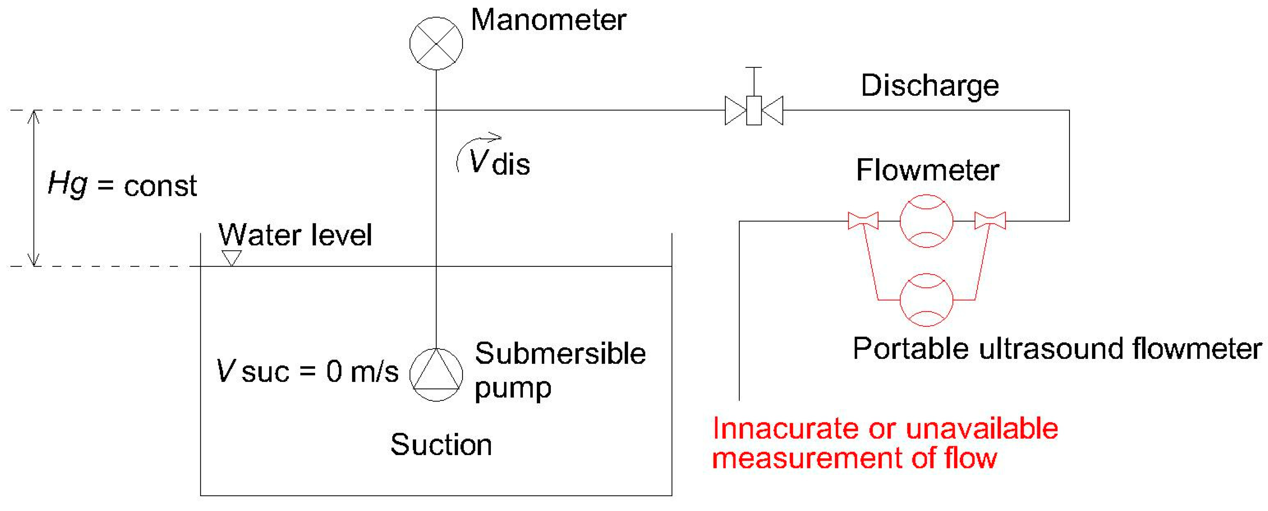
Figure 1 shows a general arrangement of elements required for the application of the proposed indirect flow rate estimation in a pump station with submersible pumps (the flowmeters depicted in red are not present at all or are possibly inaccurate due to the unsuitable place of placement in a complex pipeline configuration). The example of the placement of a portable flowmeter shown in Figure 1 is a typical example of an inappropriate position in which a significant error in flow measurement occurs (high measurement uncertainty).
Regarding the scheme from Figure 1, one should not forget about the pressure loss in the vertical section of the pipeline—the pressure measured at its top is lower than at the pump head.
Taking into account the complexity of the pipeline, the equivalent characteristics of the pump should be evaluated through the analysis of the individual system of pipes on which the pump is installed. In such a case, it is difficult to talk about the compliance or noncompliance of the measured characteristics to those given by the pump manufacturer.
In practice, there are situations where flowmeters are not installed in pumping stations, which is especially common when it comes to pumping stations of smaller capacity (usually with two pump units that do not work in a parallel configuration, but where one of them is used as a backup pump). In such cases, portable flowmeters are used to estimate the flow rate, i.e., the amount of liquid pumped in a certain period, while the choice of the position of their installation is not easy. If there are no manholes prepared in advance, it is necessary to excavate the ground around the pipeline. In such situations, this is not a common practice, but rather the flowmeter is placed in any accessible place.
For the flow-rate estimation, the pressure can be expressed in [Pa] (in [bar], where 1 bar = 105 Pa) or as a pressure head in a unit of length [m], where these two forms are related as , where is pressure [Pa] measured by the manometer at the discharge side (exactly above the pump), is the density of the water ~1000 kg/m3, g is gravitational constant ~9.81 m/sec2, while is pressure head [m]. is the correction in [m], which depends on the height difference between the position of the manometer and the water level in the tank. If the water level in the tank is constant during the experiment, the velocity at the suction side is [m/s]. The velocity at the discharge side depends on the pipeline diameter and the flow rate, which are unknown variables at the beginning. This problem can be solved either by the implementation of iterative analysis, or by proper choice of the position of the manometer (as it is shown in Section 3.2.1). Neglecting local losses from the point of fluid suction to the point of pressure measurement, total head in [m] can be estimated using Equation (1):
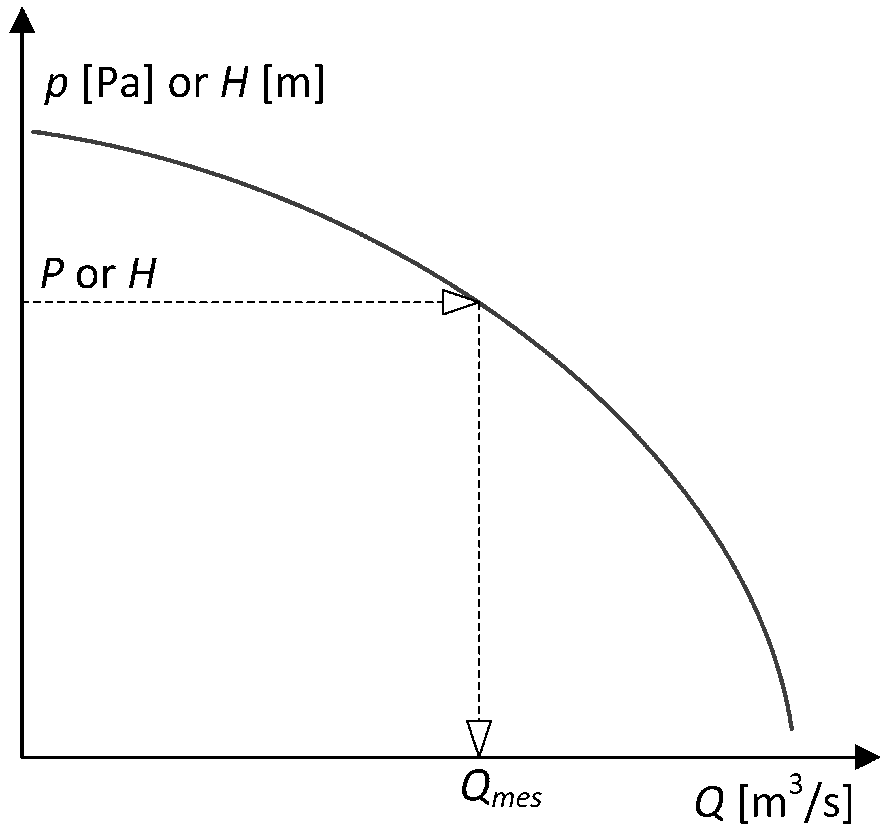
To test the approach for indirect estimation of pump flow discharge proposed here, the valve at the discharge side of the pump should be fully open. Further, the valve needs to be gradually closed in discrete steps, which changes the values of the flow and subsequently of the pressure. Therefore, for each achieved stationary operating point, the values of the pressure from the manometer should be recorded. Based on Equation (1) and graph in Figure 2, it is possible to estimate the flow rate at the discharge side of the observed pump. The curve in Figure 2 relates the total head and the flow rate and has to be obtained from the manufacturer’s catalogue or preferably from a laboratory test in advance. The possibility of discrepancy between the laboratory characteristics and characteristics from the catalogue is something that exists in reality, especially for an older pump, which has been in service for a long period of time and has been defined by valid technical standards (such as [26]). Depending on the type of pump required, minor or major deviations from the factory characteristic are permitted. The technical standard, EN ISO 9906:2012 [26], allows relatively large discrepancies between the operating characteristics of the pumps the catalogue characteristics.
Therefore, the corresponding flow can be determined indirectly for each measuring point from the known curve, (with satisfactory measurement uncertainty) for each measuring point of the pressure obtained from the manometer, as shown in Figure 2 (recalculated to ).
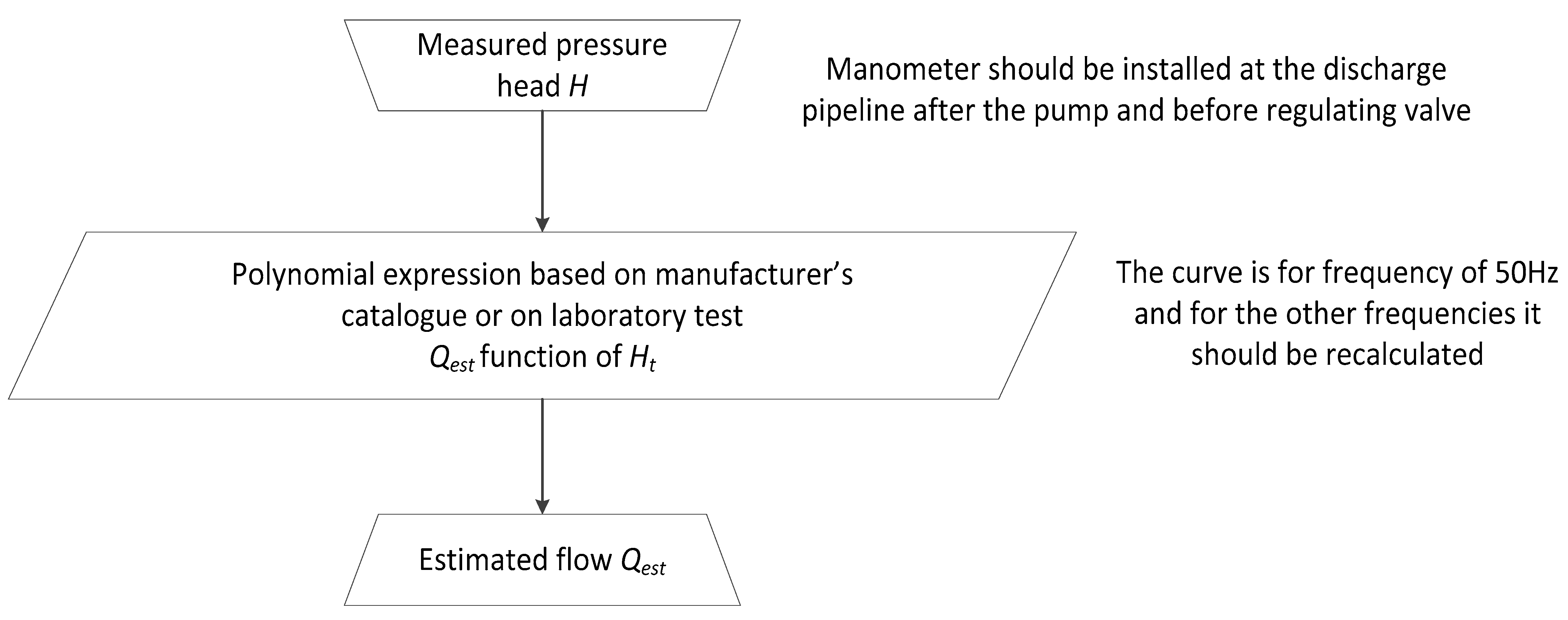
The following simple algorithm, shown in Figure 3, should be used to estimate the flow rate using the proposed approach.
3. A Practical Example
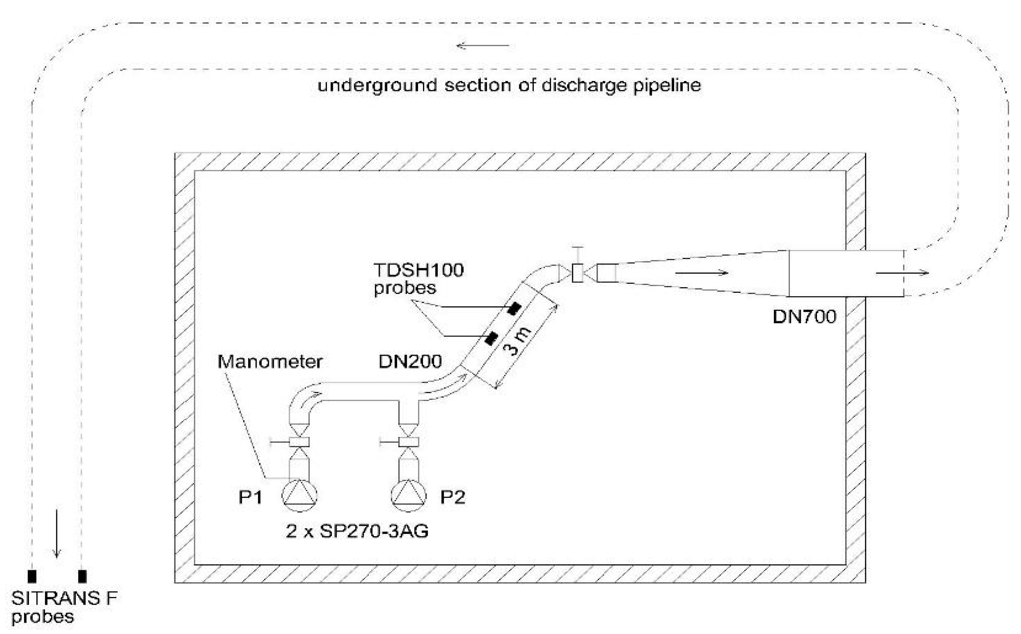
The pumping station observed in which the method has been tested has had a long history of questionable measurements of flow due to the complex geometry of the pipeline with an insufficient length of pipe where a flowmeter can be installed. Simplified diagram of the measuring pump station is shown in Figure 4 (the top view).
Due to a serious mistake during the construction process, the main discharge pipeline made of steel DN700 is not in accordance with the original project and has three elbows at short distances. Pumps are submersed in the water tank, which is placed beneath the floor of the pump station. The water level in the tank is held at a constant value. During the modernization of the pump station that has been carried out recently, the old pumps were taken out and replaced with two new submersible pumps (Grundfos SP 270-3A G). Before the installation, one of the new pumps, marked as P1 in Figure 4, had been additionally tested by the manufacturer’s laboratory.
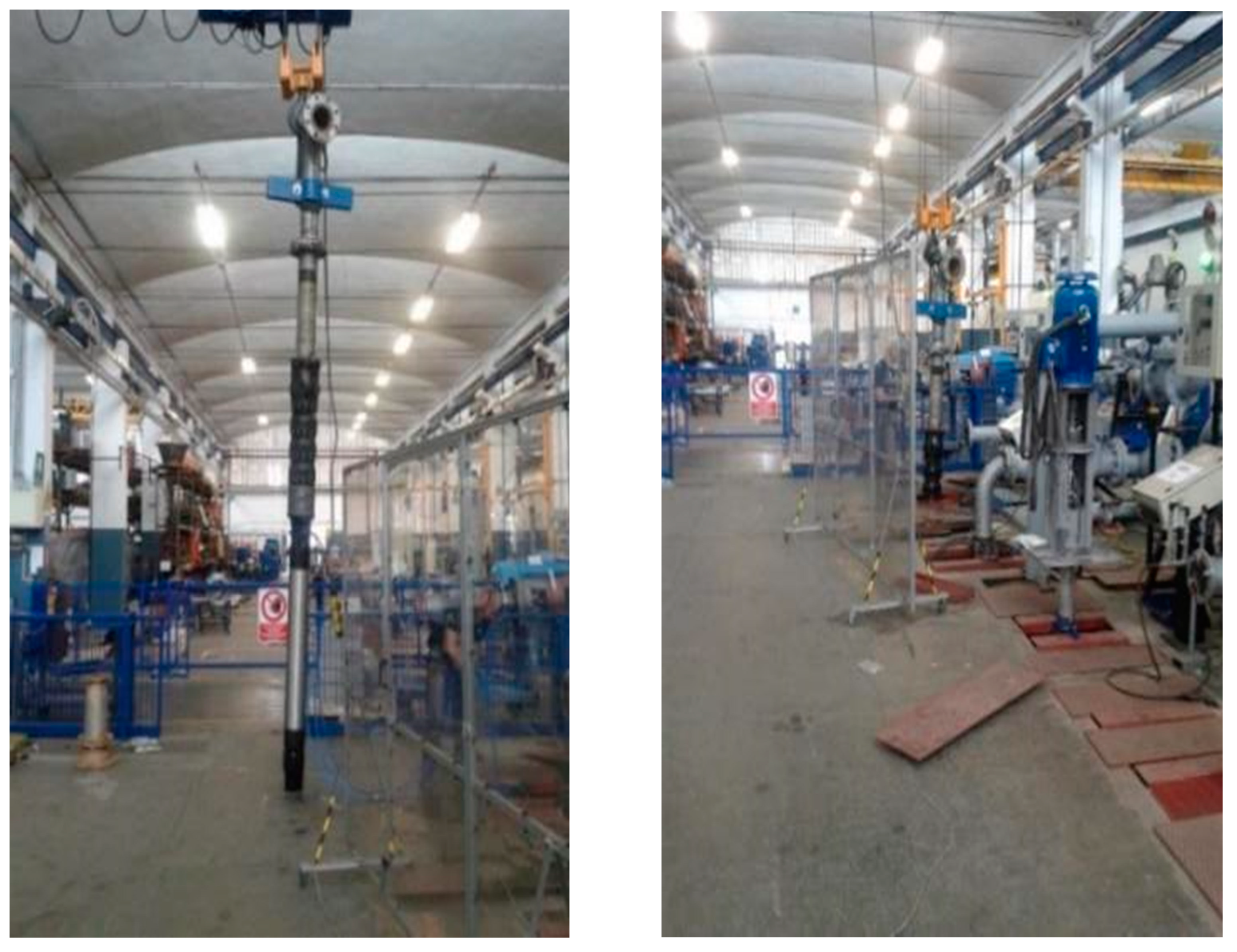
To verify the accuracy of the simplified approach proposed here in practice, flow measurements in the observed pumping station using flowmeters were performed (in further text ) and then those measured values were compared to the estimated values (in further text ). Besides, the exact curve of the observed Grundfos SP 270-3A G, which relates total head and flow was determined in the manufacturer’s laboratory (the testing of the pump in the manufacturer’s facility is shown in Figure 5, while the results are shown in Table 1). In the specific situation presented in this paper, the real characteristics of the pump recorded in the laboratory differ from those from the manufacturer’s catalogue. Furthermore, sometimes it is not possible to have a stable frequency of 50 Hz, so the actual curve from the laboratory, which relates the total head and the flow should be recalculated for the actual conditions in the observed water pumping station [27]. As we will show in the following case, the operating frequency was set to 49 Hz, to show how to recalculate a curve designed for 50 Hz.
The following equipment was used for the test in the pumping station:
- A submersible pumping unit Grundfos SP 270-3A G with a rated power of 110 kW,
- The flow was measured using a permanently installed ultrasonic flowmeter Siemens SITRANS F at the main discharge pipeline atthe observed pump station (additionally a portable ultrasonic flowmeter TDSH100 was used),
- The pressure was measured using an IDROSCAN digital manometer which was installed on the discharge side of the pump (additionally, an analogue manometer was installed),
- The frequency of the power supply tothe drive motor was regulated using a Mitsubishi F740 regulator, and
- The flow was regulated using the valve installed at the steel discharge pipe DN 200 after the pump P1.
All equipment used in our experiments has been properly tested using all common technical norms and standards required for such devices [28].
3.1. Determination of Substitute Characteristics
The purpose of this subsection is to show how the accurate curve of the observed Grundfos SP 270-3A G was determined.
3.1.1. Measuring in the Manufacturer’s Laboratory and the Recalculation for the Actual Frequency of Power Supply
The measuring in the manufacturer’s laboratory: The actual curve of the observed pump SP 270-3A G was determined experimentally in the manufacturer’s laboratory and the results are valid for power supply frequency of 50 Hz (related flows and the pressure obtained in discrete steps, which have been used to construct the curve are given in Table 1).
Laboratory tests are expensive, but they are not mandatory and do not represent what the authors suggest in every situation. In certain situations, especially when it comes to pumping units of higher power, the price of such tests may be negligible when compared to the possibilities that the user can get with the help of such tests. The fact is that pump manufacturers usually do not agree to prove the performance of pumping units at the installation sites of such pumps, because they cannot guarantee the accuracy of the measuring equipment in the pumping stations where the observed pumps have been installed. Instead, they prefer testing in an independent or the manufacturer’s laboratory. Also, the characteristics of pump units change during service life. In situations where there are flowmeters installed in pumping stations, it is not complicated to periodically perform measurements at the installation site to check and/or correct the operating characteristics of pumping units. This can usually be done as a part of planned maintenance activities in the pumping stations so that it does not increase running costs. This way, the degree of deterioration of the operating characteristics of the pumping units can be monitored. This is particularly important because their efficiency can be reduced to such an extent that it would be necessary to repair and/or to replace them.
The observed pumping station in which the method was tested has had a long history of questionable measuring of flow due to the complex geometry of the pipeline with insufficient length of pipe where a flowmeter could be installed. The installed pumps are old and due to hard exploitation, their characteristics were altered compared to those from the catalogue. Therefore, the old pumps were taken out and replaced with new pumps which have been additionally tested by the manufacturer’s laboratory (testing of the pump in the manufacturer’s facility is shown in Figure 5, while the results are shown in Table 1).
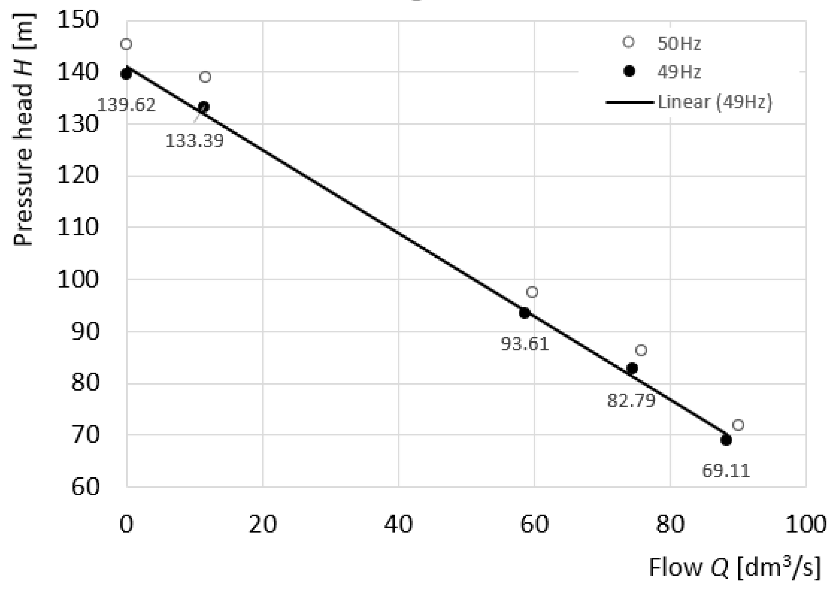
Recalculation for the actual frequency of the power supply: For an illustration of the proposed estimation of the flow in general conditions, during the test in the water pumping station where the pump has been installed, the frequency has been set to 49 Hz using a Mitsubishi F740 regulator and consequently, the curve, which relates total head and flow for such conditions has been recalculated. The corrected values have been calculated using Equation (2) and are also presented graphically in Figure 6 (based on the data points from Table 1).
Statistical calculations in the shown case are based on a limited number of measurement points from Table 1. Although this may be insufficient for a thorough analysis where the number of these points should be increased, for practical analyses, five points can be sufficient especially in cases where more data is not available such as in this case.
3.1.2. Regression Model and Statistical Analysis
To facilitate the use of the data from Table 1, the total head and the flow of the pump SP 270-3A G in our experiment can be presented graphically as given in Figure 6. The corrected graph for 49 Hz is also given in Figure 6, while the related curve based on regression analysis is given in Equation (3).
To avoid reading from the curve presented in Figure 6, it is better to use the regression formula as given in Equation (3), which gives the flow as the function of the total head for the observed pump; the data from the laboratory for 50 Hz and recalculated values for 49 Hz are in Table 1.
The data from the measurement that was used for producing of Equation (3) is given in Table 1. The relation based on the input data of Table 1 was fitted by regression analysis using Statgraphics Centurion, a statistical statistics package that performs and explains, in plain language, both basic and highly advanced statistical functions. We have tried several regression models, and we tested them using Pearson correlation and R-Squared value coefficient of determination [29,30]:
- The coefficient of determination R-Squared value denoted as R2 equals to 1.0 would indicate a perfect fit, while an R-Squared value of 0.0 would indicate the opposite case;
- The Pearson correlation coefficient is a statistic that measures the linear correlation between two variables and has a value between +1 and −1, where a value of +1 is a total positive linear correlation, 0 is no linear correlation, and −1 is total negative linear correlation.
In our particular case, a linear model is slightly more suitable for the points from Table 1, but we use the squared model because it is more general and suitable for most cases. For example, the linear model , shows the Intercept 180.147 and the Slope −1.26628 as predictors. These variables are statistically significant because their p-values equal 0.000, which are < 0.05. It also means that there is a statistically significant correlation between and at the 95% confidence level (details of the statistical analysis are given in Table 2).
Besides, it is possible to use the points from Figure 6 and Table 1 valid for the frequency of power supply of 50 Hz to construct the curve and the related function, while in that case the values of the measured flow and the pressure from the next two subsections where the frequency was 49 Hz, should be recalculated for 50 Hz, see Equation (2).
3.2. Measurement in the Observed Pumping Station
The measurements in the observed pumping station were performed for comparison with the estimated values obtained using the shown simplified method. The pressure measurement in this subsection is used as one of the input parameters and is essential for the method of flow estimation described in this technical note. However, flow measurements in this subsection are used only for comparison. The frequency of the power supply during the measurement at the water pumping station was set to 49 Hz.
3.2.1. Pressure Measurement
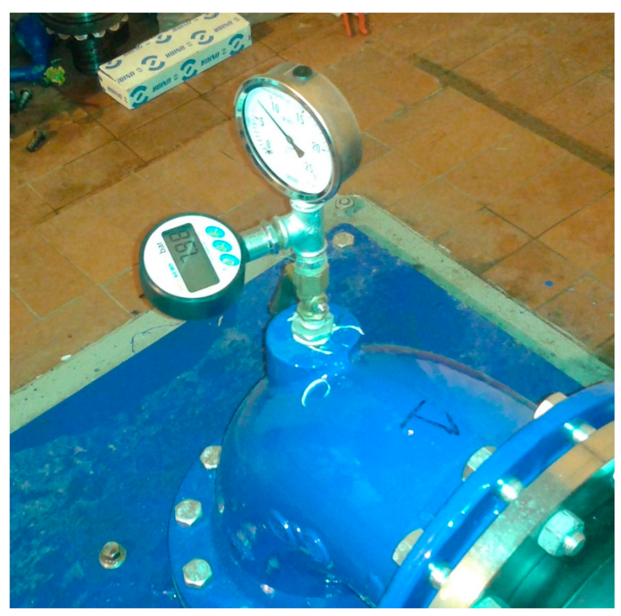
The pressure change, in the section between the pump and the valve for the regulation of flow, was monitored by IDROSCAN digital manometer with measuring range 0–50 bar (with a reading resolution of 0.01 bar and with a declared nonlinearity ±0.2%). The IDROSCAN digital manometer was placed directly on the discharge side of the pump, together with the analogue manometer (Figure 7). Because of the position of the manometers, some undesirable variation of flow can occur which can introduce a certain error of pressure measurement due to incompletely stabilized flow. However, both manometers showed the identical values of the measured pressure. It should be mentioned that due to the specific placement of the manometer (it is mounted in a special socket on the elbow of the discharge pipeline, exactly above the pump), the water velocity at the point of measuring is locally considered to be [m/s]. Thus, the measured pressure is somewhat higher than the real static pressure and includes the dynamic pressure. Due to the height difference between the position of the manometer and the water level in the tank during our experiment, correction = 1.6 m (related to Figure 1) is introduced into Equation (1).
The measured values of pressure are given in Table 3.
3.2.2. Flow Measurement
For comparison to our described method for flow friction estimation, we have performed two measurements using two different flowmeters; the permanently installed and a portable flowmeter.
Flow measurement using permanently installed ultrasonic flowmeter: The actual flow during our experiment was measured using the permanently installed Siemens SITRANS F ultrasonic flowmeter, which is shown in Figure 8.
A certain error should be predicted related to this measurement because the ultrasonic probes of Siemens SITRANS F flowmeter have been installed at the underground section of the steel pipe DN 700 with insufficient length for the flow to be fully developed, due to the lack of space (Figure 4).
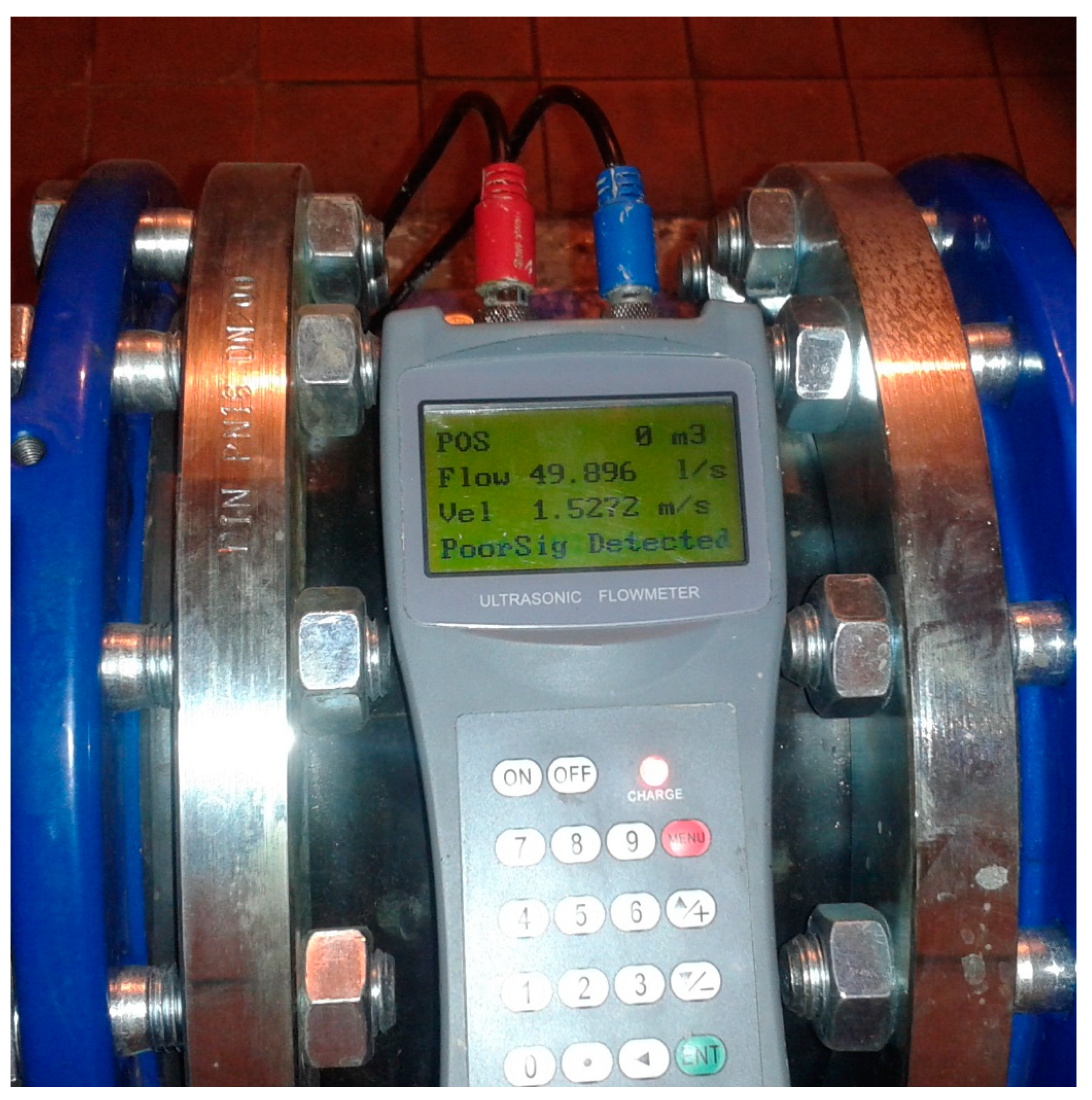
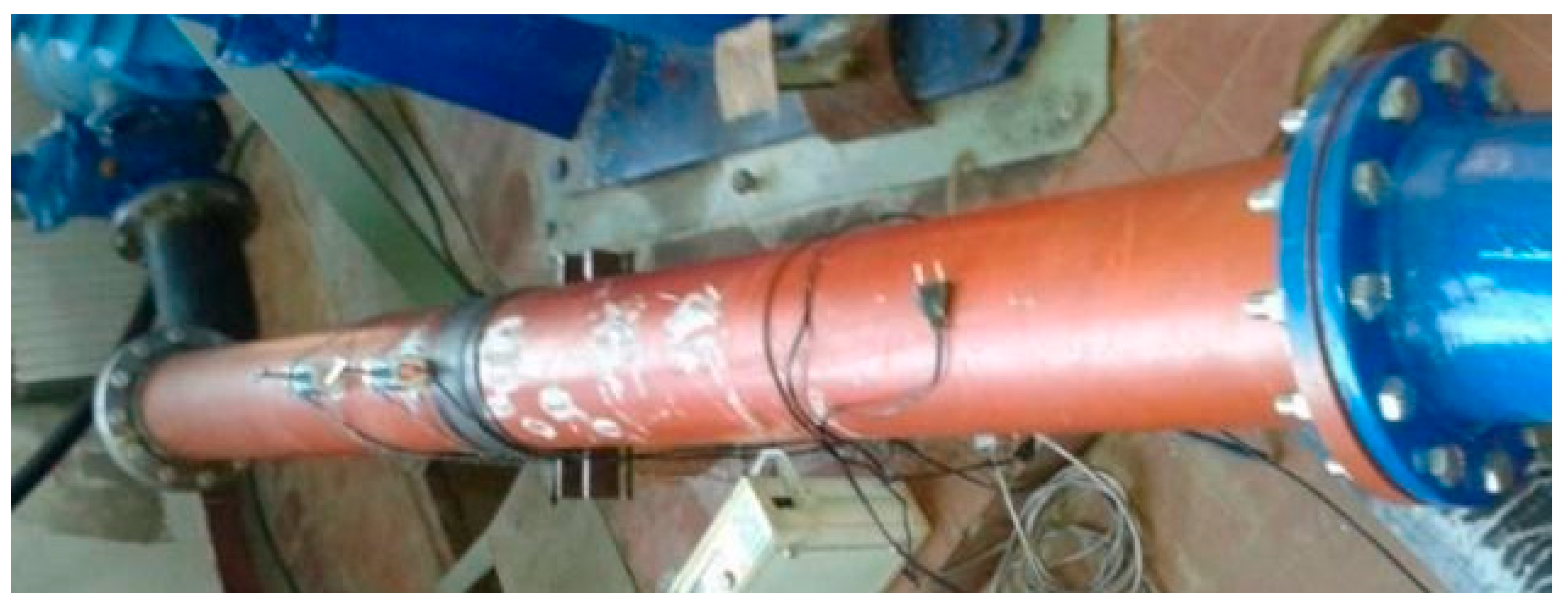
Flow measurement using portable ultrasonic flowmeter: During the experiment, additional control of flow measurement was attempted with a portable ultrasonic flowmeter TDSH100 (shown in Figure 9).
As shown in Figure 4 and Figure 10, during this additional measurement, the measuring probes were placed in the most favorable available place inside the building (on the 3 m long straight section of steel pipeline DN 200). Even so, it was not possible to obtain a satisfactory signal quality, as indicated by a clear warning on the measuring device display.
3.3. Error Estimation
The flows obtained by direct measurement using the Siemens SITRANS F flowmeter and by using the portable ultrasonic flowmeter TDSH100, and those estimated using the method here presented are shown and compared in Table 3 (the frequency of the power supply during measurement in the water pumping station was set to 49 Hz). Table 3 summarizes the measured and the estimated values from our experiment calculated using the approach proposed here. We suppose that the flow estimated using this approach is accurate, while the measured values by both flowmeters, SITRANS F and TDSH100, contain a certain level of error. The relative error of the installed flowmeters in [%] can be calculated using Equation (4):
In Equation (4), is the flow measured by flowmeters, while is the flow obtained using our method; from Figure 9 and using Equation (3). Both the measured and the estimated values of the flow are expressed in [dm3/s]. Due to the height difference between the position of the manometer and the water level in the tank during our experiment, the correction of = 1.6 m (related to Figure 1) is introduced into Equation (1).
As can be seen in Table 3, the two flowmeters used in our experiment give different results, while the permanently installed SITRANS F shows flow rates which do not differ significantly from the results obtained by using the presented approach. On the other hand, ultrasonic flowmeter TDSH100 is not reliable due to the lack of adequate position on the pipeline where the flow is fully developed and stable (the error was indicated on the display). The fact that in the example presented there was a permanently installed flowmeter made it possible to see that the portable meter does not provide accurate results, but in many other cases where there are no permanently installed measuring devices, such a conclusion cannot be made. In that sense, the results obtained by the approach proposed in this practical technical note are certainly much more reliable.
4. Conclusions
The simplified approach for flow estimation presented here can be applied in submersible pumping stations where a valve that regulates flow together with manometer is installed on the discharge pipe of the monitored pump for which the curve is known. Two main requisites are: (1) in the absence of accurate curves from manufacturers’ catalogues, which are available only for brand new pumps, the curve that relates the pump’s head and the flow should be known in advance from a laboratory, and (2) a manometer should be installed after the pump and before the regulating valve.
The approach should be used in cases where a direct measurement of the flow is not possible due to an insufficient length of the discharge pipe where the flow disturbance is so high that the readings from a flowmeter are unreliable. During the practical experiment which has been described in this technical note, the data obtained by the TDSH100 is completely unreliable and cannot be used for the flow rate measurement, while on the other hand, the permanently installed Siemens SITRANS F flowmeter gives acceptable results that can be compared with the flows estimated using our proposed simplified approach.
If there is a flowmeter installed in the pumping station, which showed accurate measured values at the beginning of the pump life due to the deterioration of the operating characteristics of the pump units there will be increasing deviations between the real flow measured. It is the deviation that should show the degree of degradation of the pump unit’s operating characteristics and show when it should be repaired or replaced.
The simplified rough method shown here can find its applications in remote rural low-income regions where water distribution is carried out through submersible pumps (installed in wells or tanks) and where flowmeters are not installed but instead pressure can be measured or estimated. Also, this approach can find application in offshore oil and gas installations where the direct flow measurement cannot always be easily performed. The simple approach can find its additional application in leak-diagnostic systems in a network of pipes, in pipelines connected with turbines, in the appropriate use of actuators, in the estimation of the density of the pumped liquid, etc. [31,32,33,34,35,36,37,38].
As the next step in the development of the proposed flow-rate estimation [39,40,41], connections between the flow and electrical quantities of the drive electric motor should be established. Electrical quantities are much easier to measure accurately, the equipment is less costly and most of these quantities are monitored and recorded on appropriate SCADA applications. Besides, as a further step, artificial intelligence can be used for error estimation in calibrating the utility of ultrasonic flowmeters. [11,42].
Author Contributions
Z.S. had the initial idea for this article and addressed the physical interpretation of the problem, described it and provided the first solution. Together with Z.S., M.R.A. and M.R., he conducted detailed experiments with pumps. D.B. and P.P. used regression techniques to provide statistical models, and they tested the method numerically. D.B. wrote a draft of this article while P.P. provided a detailed final reading of the draft. M.R.A. worked on revision of the text according to reviewers’ suggestions. All authors have read and agreed to the published version of the manuscript.
Funding
The work of M.R.A., M.R., Z.S. and D.B. has been supported by the Ministry of Education, Science, and Technological Development of the Republic of Serbia, while the work of D.B. and P.P. has been supported by the Technology Agency of the Czech Republic through the project CEET—“Center of Energy and Environmental Technologies” TK03020027.
Institutional Review Board Statement
Not applicable.
Acknowledgments
Conflicts of Interest
The authors declare no conflict of interest.
Nomenclature
| flow [m3] | |
| estimated flow rate using the proposed approach | |
| measured flow rate using flowmeters | |
| pressure [Pa] | |
| pressure at the discharge side of the pump | |
| pressure head [m], where | |
| density of fluid [kg/m3]; for water ~1000 kg/m3 | |
| gravitational constant ~9.81 m/s2 | |
| correction [m] due height difference | |
| total head [m], where | |
| total head at 49 Hz | |
| total head at 50 Hz | |
| flow rate at 49 Hz | |
| flow rate at 50 Hz | |
| relative percentage error; | |
| velocity at the suction side of pump [m/s] | |
| velocity at the discharge side of pump [m/s] |
References
- Coelho, B.; Andrade-Campos, A. Efficiency achievement in water supply systems—A review. Renew. Sustain. Energy Rev. 2014, 30, 59–84. [Google Scholar] [CrossRef]
- Lansey, K.E.; Awumah, K. Optimal pump operations considering pump switches. J. Water Resour. Plan. Manag. 1994, 120, 17–35. [Google Scholar] [CrossRef]
- Chai, H.; Yang, G.; Wu, G.; Bai, G.; Li, W. Research on flow characteristics of straight line conjugate internal meshing gear pump. Processes 2020, 8, 269. [Google Scholar] [CrossRef] [Green Version]
- Koury Costa, G.; Sepehri, N. A critical analysis of valve-compensated hydrostatic actuators: Qualitative investigation. Actuators 2019, 8, 59. [Google Scholar] [CrossRef] [Green Version]
- Smith, I. Measuring Pump Station Performance. 74th Annual Water Industry Engineers and Operators’ Conference, Bendigo Exhibition Centre, 6 to 8 September 2011. Available online: http://www.wioa.org.au/conference_papers/2011_vic/documents/Ian_Smith.pdf (accessed on 7 July 2020).
- Luo, Y.; Sun, H.; Yuan, S.Q.; Yu, Z.S. Experimental study of transducer harmonics effect on pump unit energy consumption. Chem. Eng. Trans. 2015, 46, 973–978. [Google Scholar]
- Torres, L.; Jiménez-Cabas, J.; González, O.; Molina, L.; López-Estrada, F.-R. Kalman filters for leak diagnosis in pipelines: Brief history and future research. J. Mar. Sci. Eng. 2020, 8, 173. [Google Scholar] [CrossRef] [Green Version]
- Mandard, E.; Kouame, D.; Battault, R.; Remenieras, J.P.; Patat, F. Methodology for developing a high-precision ultrasound flowmeter and fluid velocity profile reconstruction. IEEE Trans. Ultrason. Ferroelectr. Freq. Control 2008, 55, 161–172. [Google Scholar] [CrossRef] [PubMed]
- Zhang, H.; Guo, C.; Lin, J. Effects of velocity profiles on measuring accuracy of transit-time ultrasonic flowmeter. Appl. Sci. 2019, 9, 1648. [Google Scholar] [CrossRef] [Green Version]
- Simão, M.; Besharat, M.; Carravetta, A.; Ramos, H.M. Flow velocity distribution towards flowmeter accuracy: CFD, UDV, and field tests. Water 2018, 10, 1807. [Google Scholar] [CrossRef] [Green Version]
- Barbariol, T.; Feltresi, E.; Susto, G.A. Self-diagnosis of multiphase flowmeters through machine learning-based anomaly detection. Energies 2020, 13, 3136. [Google Scholar] [CrossRef]
- Taha, A.W.; Mahardani, M.; Sharma, S.; Arregui, F.; Kennedy, M. Impact of float-valves on water meter performance under intermittent and continuous supply conditions. Resour. Conserv. Recycl. 2020, 163, 105091. [Google Scholar] [CrossRef]
- Pimenta, B.D.; Robaina, A.D.; Peiter, M.X.; Kirchner, J.H.; Mezzomo, W.; Torres, R.R. Performance of ultrasonic flowmeter in different vinyl polychloride pipes. IRRIGA 2018, 23, 87–95. [Google Scholar] [CrossRef]
- Prettyman, J.B.; Johnson, M.C.; Barfuss, S.L. Comparison of selected differential-producing, ultrasonic, and magnetic flowmeters. J. Am. Water Work. Assoc. 2016, 108, E39–E49. [Google Scholar] [CrossRef] [Green Version]
- Hogendoorn, J.; Hofstede, H.; van Brakel, P.; Boer, A. How accurate are ultrasonic flowmeters in practical conditions; beyond the calibration. In Proceedings of the 29th International North Sea Flow Measurement Workshop, Tonsberg, Norway, 25–28 October 2011; Available online: https://nfogm.no/wp-content/uploads/2019/02/2011-12-How-Accurate-are-Ultrasonic-Flowmeters-in-Practical-Conditions-Hogendoorn-Krohne.pdf (accessed on 4 October 2020).
- Sun, B.; Chen, S.; Liu, Q.; Lu, Y.; Zhang, C.; Fang, H. Review of sewage flow measuring instruments. Ain Shams Eng. J. 2021. [Google Scholar] [CrossRef]
- Martim, A.L.; Dalfré Filho, J.G.; De Lucca, Y.D.; Genovez, A.I. Electromagnetic flowmeter evaluation in real facilities: Velocity profiles and error analysis. Flow Meas. Instrum. 2019, 66, 44–49. [Google Scholar] [CrossRef]
- Ge, L.; Chen, J.; Tian, G.; Zeng, W.; Huang, Q.; Hu, Z. Study on a new electromagnetic flow measurement technology based on differential correlation detection. Sensors 2020, 20, 2489. [Google Scholar] [CrossRef]
- Munasinghe, N.; Paul, G. Ultrasonic-based sensor fusion approach to measure flow rate in partially filled pipes. IEEE Sens. J. 2020, 20, 6083–6090. [Google Scholar] [CrossRef]
- Lv, R.Q.; Zheng, H.K.; Zhao, Y.; Gu, Y.F. An optical fiber sensor for simultaneous measurement of flow rate and temperature in the pipeline. Opt. Fiber Technol. 2018, 45, 313–318. [Google Scholar] [CrossRef]
- Leontidis, V.; Cuvier, C.; Caignaert, G.; Dupont, P.; Roussette, O.; Fammery, S.; Nivet, P.; Dazin, A. Experimental validation of an ultrasonic flowmeter for unsteady flows. Meas. Sci. Technol. 2018, 29, 045303. [Google Scholar] [CrossRef] [Green Version]
- Mutikanga, H.E.; Sharma, S.K.; Vairavamoorthy, K. Investigating water meter performance in developing countries: A case study of Kampala, Uganda. Water SA 2011, 37, 567–574. [Google Scholar] [CrossRef] [Green Version]
- Criminisi, A.; Fontanazza, C.M.; Freni, G.; Loggia, G.L. Evaluation of the apparent losses caused by water meter under-registration in intermittent water supply. Water Sci. Technol. 2009, 60, 2373–2382. [Google Scholar] [CrossRef]
- Formato, A.; Guida, D.; Ianniello, D.; Villecco, F.; Lenza, T.L.; Pellegrino, A. Design of delivery valve for hydraulic pumps. Machines 2018, 6, 44. [Google Scholar] [CrossRef] [Green Version]
- Formato, G.; Romano, R.; Formato, A.; Sorvari, J.; Koiranen, T.; Pellegrino, A.; Villecco, F. Fluid-structure interaction modeling applied to peristaltic pump flow simulations. Machines 2019, 7, 50. [Google Scholar] [CrossRef] [Green Version]
- Technical Standard EN ISO 9906:2012, Rotodynamic Pumps—Hydraulic Performance Acceptance Tests—Grades 1, 2 and 3. Available online: https://www.iso.org/standard/41202.html (accessed on 12 March 2021).
- Wang, G.; Song, L. Performance assessment of variable frequency drives in heating, ventilation, and air-conditioning systems. Sci. Technol. Built Environ. 2018, 24, 1075–1083. [Google Scholar] [CrossRef]
- Brkić, D.; Praks, P. Proper use of technical standards in offshore petroleum industry. J. Mar. Sci. Eng. 2020, 8, 555. [Google Scholar] [CrossRef]
- MathWorks Help Center, Linear Regression. Available online: https://www.mathworks.com/help/matlab/data_analysis/linear-regression.html (accessed on 5 September 2020).
- González-Manteiga, W.; Crujeiras, R.M. An updated review of goodness-of-fit tests for regression models. Test 2013, 22, 361–411. [Google Scholar] [CrossRef] [PubMed]
- Bermúdez, J.-R.; López-Estrada, F.-R.; Besançon, G.; Valencia-Palomo, G.; Torres, L.; Hernández, H.-R. Modeling and Simulation of a Hydraulic Network for Leak Diagnosis. Math. Comput. Appl. 2018, 23, 70. [Google Scholar] [CrossRef] [Green Version]
- Fomicheva, M.; Müller, W.H.; Vilchevskaya, E.N.; Bessonov, N. Funnel flow of a navier-stokes-fluid with potential applications to micropolar media. Facta Univ. Ser. Mech. Eng. 2019, 17, 255–267. [Google Scholar] [CrossRef]
- Xue, Z.; Tao, L.; Fuchun, J.; Riehle, E.; Xiang, H.; Bowen, N.; Singh, R.P. Application of acoustic intelligent leak detection in an urban water supply pipe network. J. Water Supply Res. Technol. AQUA 2020, 69, 512–520. [Google Scholar] [CrossRef]
- Benad, J. Numerical methods for the simulation of deformations and stresses in turbine blade fir-tree connections. Facta Univ. Ser. Mech. Eng. 2019, 17, 1–15. [Google Scholar] [CrossRef] [Green Version]
- Santos-Ruiz, I.; López-Estrada, F.-R.; Puig, V.; Valencia-Palomo, G. Simultaneous optimal estimation of roughness and minor loss coefficients in a pipeline. Math. Comput. Appl. 2020, 25, 56. [Google Scholar] [CrossRef]
- Gøytil, P.H.; Padovani, D.; Hansen, M.R. A novel solution for the elimination of mode switching in pump-controlled single-rod cylinders. Actuators 2020, 9, 20. [Google Scholar] [CrossRef] [Green Version]
- Nabil, T.; Alhaddad, F.; Dawood, M.; Sharaf, O. Experimental and numerical investigation of flow hydraulics and pipe geometry on leakage behaviour of laboratory water network distribution systems. J. Adv. Res. Fluid Mech. Therm. Sci. 2020, 75, 20–42. [Google Scholar] [CrossRef]
- Sadeghi, H.; Poshtan, J.; Poulsen, N.K.; Niemann, H. Estimating the density of fluid in a pipeline system with an electropump. J. Pipeline Syst. Eng. Pract. 2018, 9, 06018002. [Google Scholar] [CrossRef]
- Brkić, D.; Praks, P. Accurate and Efficient Explicit Approximations of the Colebrook Flow Friction Equation Based on the Wright ω-Function. Mathematics 2019, 7, 34. [Google Scholar] [CrossRef] [Green Version]
- Praks, P.; Brkić, D. Review of new flow friction equations: Constructing Colebrook’s explicit correlations accurately. Rev. Int. Métodos Numéricos Para Cálculo Diseño Ing. 2020, 36, 41. [Google Scholar] [CrossRef]
- Praks, P.; Brkić, D. Suitability for coding of the Colebrook’s flow friction relation expressed through the Wright ω-function. Rep. Mech. Eng. 2020, 1, 174–179. [Google Scholar] [CrossRef]
- Yazdanshenasshad, B.; Safizadeh, M.S. Neural-network-based error reduction in calibrating utility ultrasonic flowmeters. Flow Meas. Instrum. 2018, 64, 54–63. [Google Scholar] [CrossRef]
Figure 1.
The layout of the elements required for flow rate estimation.

Figure 2.
Indirect determination of flow at the measuring point based on the curve, which relates total head and flow .
Figure 2.
Indirect determination of flow at the measuring point based on the curve, which relates total head and flow .

Figure 3.
A simple algorithm for estimation of discharge flow.

Figure 4.
Simplified diagram of the pump station.

Figure 5.
Testing of SP 270-3A G pump in the laboratory.

Figure 6.
The experimentally determined curve which relates pressure head and flow of the SP 270-3A G pump recalculated for 49 Hz.
Figure 6.
The experimentally determined curve which relates pressure head and flow of the SP 270-3A G pump recalculated for 49 Hz.

Figure 7.
IDROSCAN digital manometer together with the analogue manometer.

Figure 8.
Ultrasonic flowmeter Siemens SITRANS F.

Figure 9.
Portable ultrasonic flowmeter TDSH100.

Figure 10.
Measuring probes of the portable ultrasonic flowmeter TDSH100.


Table 1.
Values for the curve that relates total head and flow of the SP 270-3A G pump measured in the laboratory at 50 Hz and recalculated for 49 Hz.
Table 1.
Values for the curve that relates total head and flow of the SP 270-3A G pump measured in the laboratory at 50 Hz and recalculated for 49 Hz.
| 50 Hz | |||||
| [dm3/s] | 0 | 11.67 | 59.88 | 75.84 | 90.08 |
| [m] | 145.38 | 138.89 | 97.47 | 86.2 | 71.96 |
| 49 Hz | |||||
| [dm3/s] | 0 | 11.44 | 58.68 | 74.32 | 88.28 |
| [m] | 139.62 | 133.39 | 93.61 | 82.79 | 69.11 |
Table 2.
Comparison of alternative models obtained by the Statgraphics Centurion software using Pearson correlation and R-Squared value coefficient of determination.
Table 2.
Comparison of alternative models obtained by the Statgraphics Centurion software using Pearson correlation and R-Squared value coefficient of determination.
| Model | Correlation | R-Squared |
|---|---|---|
| Linear | −0.9991 | 99.82% |
| Squared- | −0.9980 | 99.60% |
| Squared- reciprocal- | 0.9978 | 99.56% |
| Square root- | −0.9977 | 99.53% |
| Logarithmic- | −0.9945 | 98.91% |
| Squared- logarithmic- | −0.9920 | 98.41% |
| Squared- square root- | −0.9866 | 97.34% |
| Reciprocal- | 0.9822 | 96.47% |
| Squared- | −0.9799 | 96.03% |
| Square root- squared- | −0.9760 | 95.26% |
| Square root- | −0.9663 | 93.37% |
| Double squared | −0.9643 | 92.98% |
| Double square root | −0.9592 | 92.01% |
| Square root- logarithmic- | −0.9504 | 90.33% |
| Square root- reciprocal- | −0.9269 | 85.92% |
Table 3.
Values obtained by using the presented method in the observed pumping station.
| Directly Measured | Estimated | Error | ||||
|---|---|---|---|---|---|---|
| -SITRANS F [dm3/s] | -TDSH100 [dm3/s] | |||||
| 8.00 | 81.71 | 79.5 | 64.2 | 74.13 | 6.8% | −15.5% |
| 8.10 | 82.73 | 77.5 | 61.2 | 72.94 | 5.9% | −19.2% |
| 8.19 | 83.65 | 77.0 | 70.0 | 71.87 | 6.7% | −2.7% |
| 8.31 | 84.88 | 74.8 | 67.0 | 70.44 | 5.8% | −5.1% |
| 8.44 | 86.21 | 73.3 | 54.4 | 68.88 | 6.0% | −26.6% |
| 8.60 | 87.84 | 70.8 | 50.4 | 66.96 | 5.4% | −32.9% |
| 8.80 | 89.88 | 67.0 | 46.8 | 64.54 | 3.7% | −37.9% |
| 9.09 | 92.85 | 62.5 | 44.0 | 61.01 | 2.4% | −38.7% |
| 9.59 | 97.95 | 54.5 | 34.3 | 54.84 | 0.6% | −59.9% |
is calculated using Equation (1) where = 1.6 m.
Publisher’s Note: MDPI stays neutral with regard to jurisdictional claims in published maps and institutional affiliations. |
© 2021 by the authors. Licensee MDPI, Basel, Switzerland. This article is an open access article distributed under the terms and conditions of the Creative Commons Attribution (CC BY) license (http://creativecommons.org/licenses/by/4.0/).
Share and Cite
MDPI and ACS Style
Rašić Amon, M.; Radić, M.; Stajić, Z.; Brkić, D.; Praks, P. Simplified Indirect Estimation of Pump Flow Discharge: An Example from Serbia. Water 2021, 13, 796. https://doi.org/10.3390/w13060796
AMA Style
Rašić Amon M, Radić M, Stajić Z, Brkić D, Praks P. Simplified Indirect Estimation of Pump Flow Discharge: An Example from Serbia. Water. 2021; 13(6):796. https://doi.org/10.3390/w13060796
Chicago/Turabian StyleRašić Amon, Milica, Milan Radić, Zoran Stajić, Dejan Brkić, and Pavel Praks. 2021. "Simplified Indirect Estimation of Pump Flow Discharge: An Example from Serbia" Water 13, no. 6: 796. https://doi.org/10.3390/w13060796
Note that from the first issue of 2016, this journal uses article numbers instead of page numbers. See further details here.