Integration of the Analytical Hierarchy Process and GIS Spatial Distribution Model to Determine the Possibility of Runoff Water Harvesting in Dry Regions: Wadi Watir in Sinai as a Case Study

Abstract

Runoff water harvesting (RWH) is considered as an important tool for overcoming water scarcity in arid and semi-arid regions. The present work focuses on identifying potential RWH sites in the Wadi Watir watershed in the south-eastern part of the Sinai Peninsula. This was carried out by means of significant integration of the analytical hierarchy process (AHP), distributed spatial model, geographical information system (GIS), watershed modeling system (WMS), and remote sensing techniques (RS). This integration of modern research tools has its own bearing on the accurate identification of optimum RWH sites, which could be relied upon in developmental planning for arid environments. Eight effective RWH parameters were chosen to apply a multi-parametric decision spatial model (MPDSM), namely the overland flow distance, volume of annual flood, drainage density, maximum flow distance, infiltration number, watershed slope, watershed area and watershed length. These parameters were used within ArcGIS 10.1© as thematic layers to build a distributed hydrological spatial model. The weights and ranks of each model parameter were assigned according to their magnitude of contribution in the RWH potentiality mapping using a pairwise correlation matrix verified by calculating the consistency ratio (CR), which governs the reliability of the model application. The CR value was found to be less than 0.1 (0.069), indicating acceptable consistency and validity for use. The resulting MPDSM map classified the watershed into five categories of RWH potential, ranging from very low to very high. The high and very high classes, which are the most suitable for RWH structures, make up approximately 33.24% of the total watershed area. Accordingly, four retention dams and seven ground cisterns (tanks) were proposed in these areas to collect and store the runoff water, whereby these proposed RWH structures were chosen according to the soil type and current land-use pattern. The resulting MPDSM map was validated using a topographic wetness index (TWI) map, created for the watershed. This integrative and applied approach is an important technique which can be applied in similar arid environments elsewhere.

1. Introduction

Water shortage could potentially cause a socio-economic crisis in Egypt. Drought management and sustainable agricultural production in arid and semi-arid areas depend heavily on careful planning in exploring and exploiting water resources for human needs. In arid and semi-arid regions, intense rainfall causes high runoff water, with resultant flooding which poses problems for the human population and the infrastructure of communities in these areas [1,2,3,4]. These areas must be carefully managed in order to mitigate against the potential risks of flood events.

The Sinai Peninsula is a strategic part of Egypt because of its historical importance, tourist sites, natural resources and new development activities. The Peninsula is one of the arid regions of the country and is experiencing a worsening water crisis. Hence, water resource management systems are very important in this region. Many watersheds in the Sinai Peninsula are characterized by flood activity, such as Wadi Watir, Wadi Dahab and Wadi Fieran. These floods cause serious threats and frequent disastrous results for infrastructure, human life and property. Suitable runoff water harvesting (RWH) techniques should be applied to these watersheds to preserve the many important economic and tourism advantages of cities such as Nuweiba, Dahab and Al-Tur, and to support many thousands of people in this area with sufficient quantities of water.

RWH is an important technique which helps provide surface water for different uses in arid regions, as well as increasing opportunities for recharging groundwater reserves, mitigating the risk of flash floods and implementing various development activities, such as rain-fed local agricultural areas and ground cisterns for drinking-water purposes. RWH can minimize the excess loss of potable water in landscape sanitation and irrigation [5,6]. There is a vital need to manage the resultant runoff water in arid and semi-arid environments with unpredictable rainfall patterns [7]. Runoff water from rainfall events is a promising water resource and can be utilized for different demands if it is correctly harvested [8]. As a matter of fact, determining the RWH potential is opposite to the concept of groundwater potential. Some techniques of water harvesting involve using runoff water for recharging groundwater aquifer systems, but RWH was originally intended to have its own bearing on the overall enhancement of local groundwater regimes, improving moisture conditions and raising the soil productivity.

Various watershed models (empirical, conceptual or physically-based) as well as remote sensing (RS) and geographic information system (GIS) are used to resolve watershed problems such as flash flood hazards and to determine the optimal locations for RWH structures and recharging groundwater. Watershed modeling system (WMS) is usually applied as simple lumped, distributed and semi-distributed models [7]. Lumped models refer to each watershed as a monolithic unit, in which all hydrological parameters of the watershed are spatially linked together to generate uniformity through the watershed [8]. Lumped models assume uniform distribution of rainfall over a watershed time period [9]. Semi-distributed models were developed to represent the spatial diversity of watershed characteristics. The watershed is supposed to divide into sub-watersheds, each with its own hydrological parameter. Vieux et al. [10] stated that semi-distributed models represent spatially variable parameters or conditions as a series of sub-watersheds, each having uniform characteristics. These models can be formulated by means of the Hydrological Modeling System (HEC-HMS) or Hydrological Simulation-Fortran Program (HSPF) using the hydrological response unit (HRU) [11]. Distributed models are the latest extension of lumped and semi-distributed models. These models represent the physical properties and spatial heterogeneity of the watershed. They are based on dividing the watershed into elementary grid cells and applying physical equations to simulate water pooling processes [12]. Flows are run from each grid cell to another, where water drains through the watershed, allowing these models to simulate the heterogeneity of the watershed in each cell of the grid [13]. Distributed models are used to represent the spatial diversity of precipitation, soil type and land use within each watershed [14]. Distributed modeling is an active area of research due to the increasing power of modern computers and the increased capabilities of GISs [13].

Previous research studies used morphometric, hydrological parameters for flashflood mitigation and watershed management, e.g., [5,15,16,17,18]. Elewa et al. [17] determined the flood potential of Wadi El-Arish by applying a semi-distributed model for watershed morphometric parameters. AbuZied et al. [18] identified the geospatial assessment of sudden flood risk in the Nuweiba area using morphometric and hydrological factors within RS and GIS techniques. Mishra et al. [19] applied the soil and water assessment model to the morphological characteristics of sub-watersheds to determine their priorities.

The purpose of this work is to identify potential sites for RWH in the Wadi Watir watershed in order to mitigate flash floods. As the input for the present work, RS, GISs, WMSs, the spatial distributed model and analytical hierarchy processes (AHPs) were integrated for RWH potentiality mapping. These tools play an imperative role in identifying and analyzing hydro-morphometric information for watersheds.

Hydro-morphometric parameters were calculated using WMS, RS and GIS techniques based on climatic data, geologic maps, the digital elevation model (DEM) and Landsat Enhanced Thematic Mapper Plus (ETM ⁺) satellite images for Wadi Watir. These parameters were used as thematic layers within ArcGIS 10.1© software (Esri, Redlands California, United States) [20] to perform multi-parametric decision spatial models (MPDSMs) to determine the possibility of harvesting runoff water. The model applied eight parameters: watershed area (A), watershed length (BL), maximum flow distance (MFD), watershed slope (BS), overland flow distance (OFD), watershed infiltration number (IF), drainage density (DD) and volume of annual flood (VAF). The weights and ranks of these parameters were determined by applying the AHP technique. This technique is used to justify the weights of the model’s variables based on expert judgment [21]. AHP has wide applicability in various fields due to its flexibility, simplicity, ease of handling and successful integration with various techniques [22]. The method is based on a pairwise correlation matrix to compare different parameters and determine their weights. AHP offers solutions to many complex multi-parametric, multi-period and hierarchical decision-making problems [23]. Malczewski et al. [24] used the AHP technique with linear programming in land-use planning. Jiang et al. [25] and Taheri et al. [26] used the same method to identify zones subject to sinkholes. Nekhay et al. [27] assessed the suitability of olive farms to restore wildlife habitats using AHP and GIS techniques.

Drainage areas and hydro-morphometric parameters of Wadi Watir were identified using the watershed modeling system in WMS 8© software (Aquaveo LLC, U.S. Army Corps of Engineers, Engineer Research & Development Center) [28]. The volume of the annual flood was calculated by applying the Soil Conservation Service Curve Number method (SCS-CN) [29] and the Finkel method [30]. In the present work, the Wadi Watir watershed occupying the south-eastern part of the Sinai Peninsula was chosen as a case study to apply the proposed MPDSM (Figure 1). The results of this model will assist decision-makers in proposing effective RWH structures and implementing micro-catchment rain-fed agriculture. The Wadi Watir watershed is characterized by substantial floods, which occur sporadically in autumn or spring and often cause extensive damage to the major roads crossing the Wadi and many infrastructure items in the vicinity [31]. Effective runoff in South Sinai can be achieved through storms exceeding 10 mm [32]. Moore et al. [33] suggested that in the Middle East, 10 mm in the coastal areas and up to 50 mm in the highlands often cause sudden flooding.

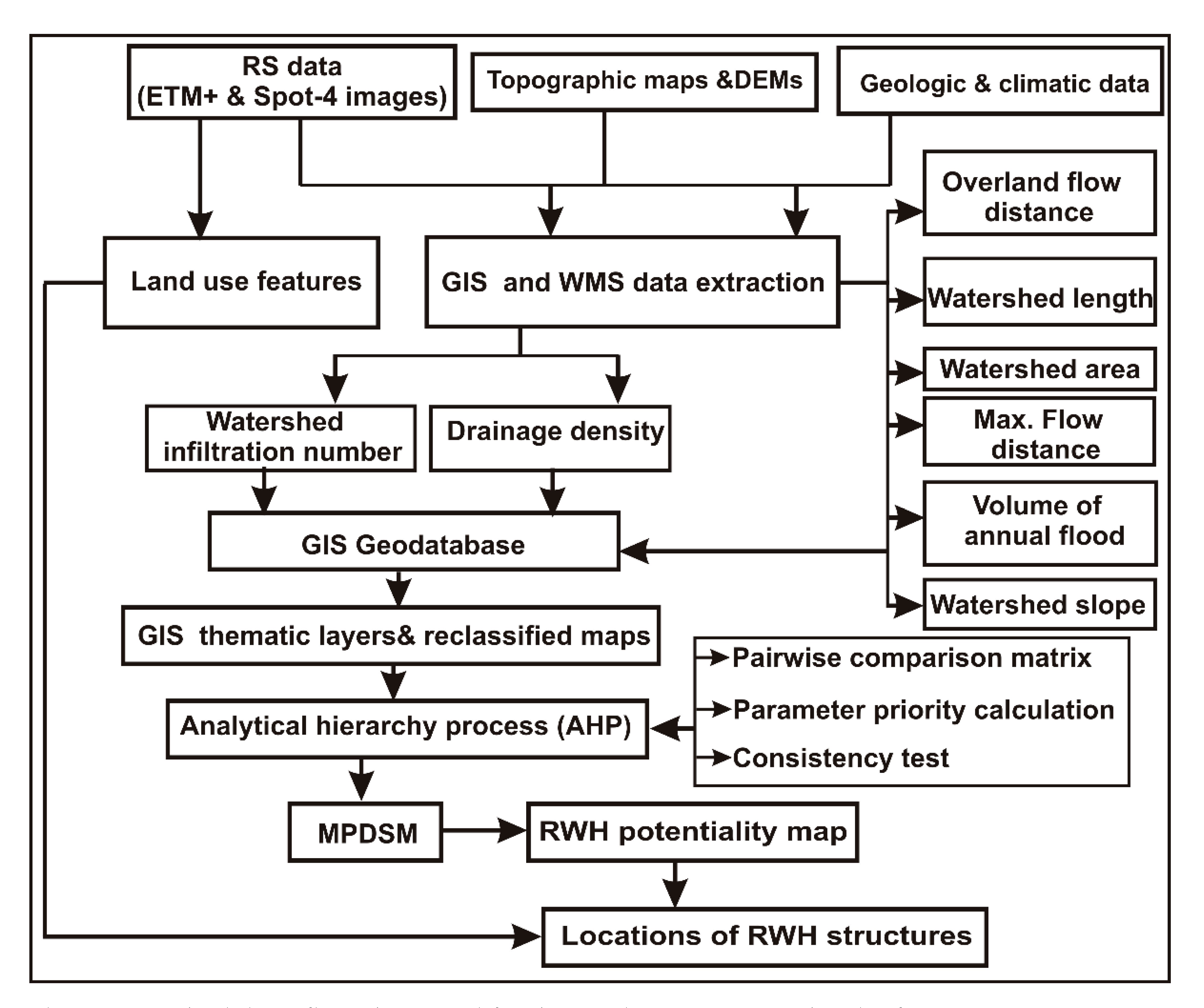
2. Materials and Methods

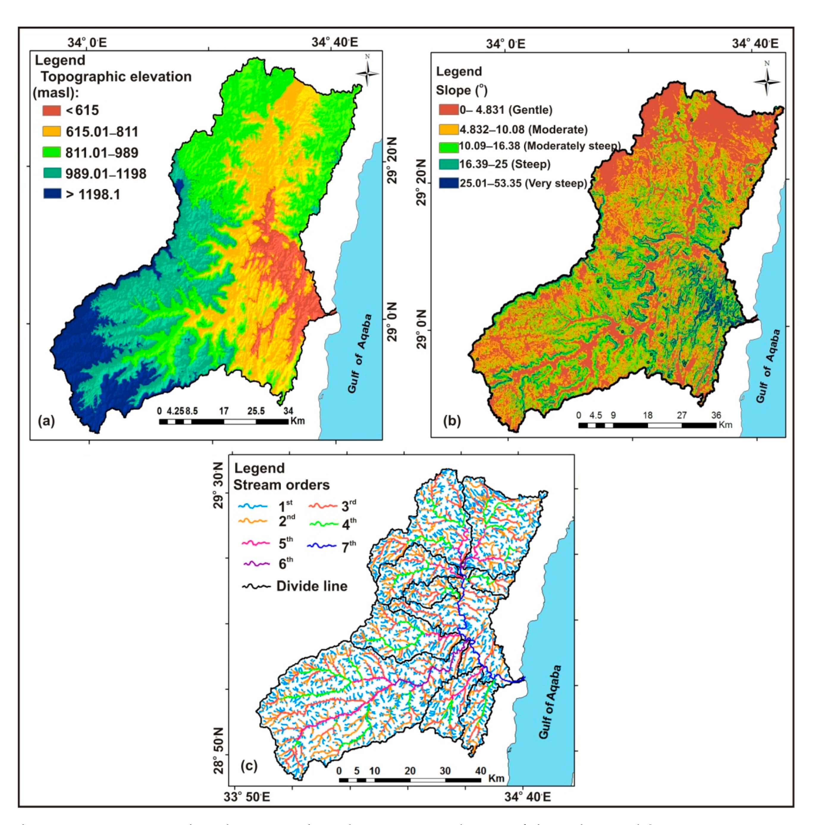
2.1. Study Area

Wadi Watir is located in the south-eastern part of the Sinai Peninsula, between longitudes 34°38′ and 34°41′ E and latitudes 28°40′ and 29°30′ N (Figure 1). It is one of the main and active watersheds in the Gulf of Aqaba drainage system, covering an area of 3515 km². Its main channel runs north–south for about 40 km and then bends slightly in a north-northwest–south-southeast direction for approximately 25 km, finally entering the Gulf of Aqaba near the city of Nuweiba, which is one of the most important tourist and historical cities in the Sinai Peninsula, and therefore needs large quantities of water, which may be obtained by applying RWH technologies. The watershed is characterized by steep hills rising up to 1600 m above sea level (ASL) (Figure 2a). The hills are mainly composed of impermeable rocks, while the stream beds are covered with a highly permeable mix of gravel and sand. The watershed is characterized by great slope diversity, as it varies between gentle to very steep slopes (Figure 2b). It consists of ten sub-watersheds, joining the trunk channel from east and west at highly acute angles and varying in their orders from the fourth to the seventh (Figure 2c). The watershed area received an average rainfall of 54.87 mm/year between 1998 and 2007 [34], and it was estimated by [35] as 46.96 mm/year between 1960 and 1990. The Wadi Watir watershed is characterized by precipitation which is sufficient to produce a large amount of runoff water, feeding the famous Ain Furtaga spring with a continuous flow all year round. This spring is one of the largest in the Sinai Peninsula and is widely used by the local Bedouin for drinking water and limited agriculture.

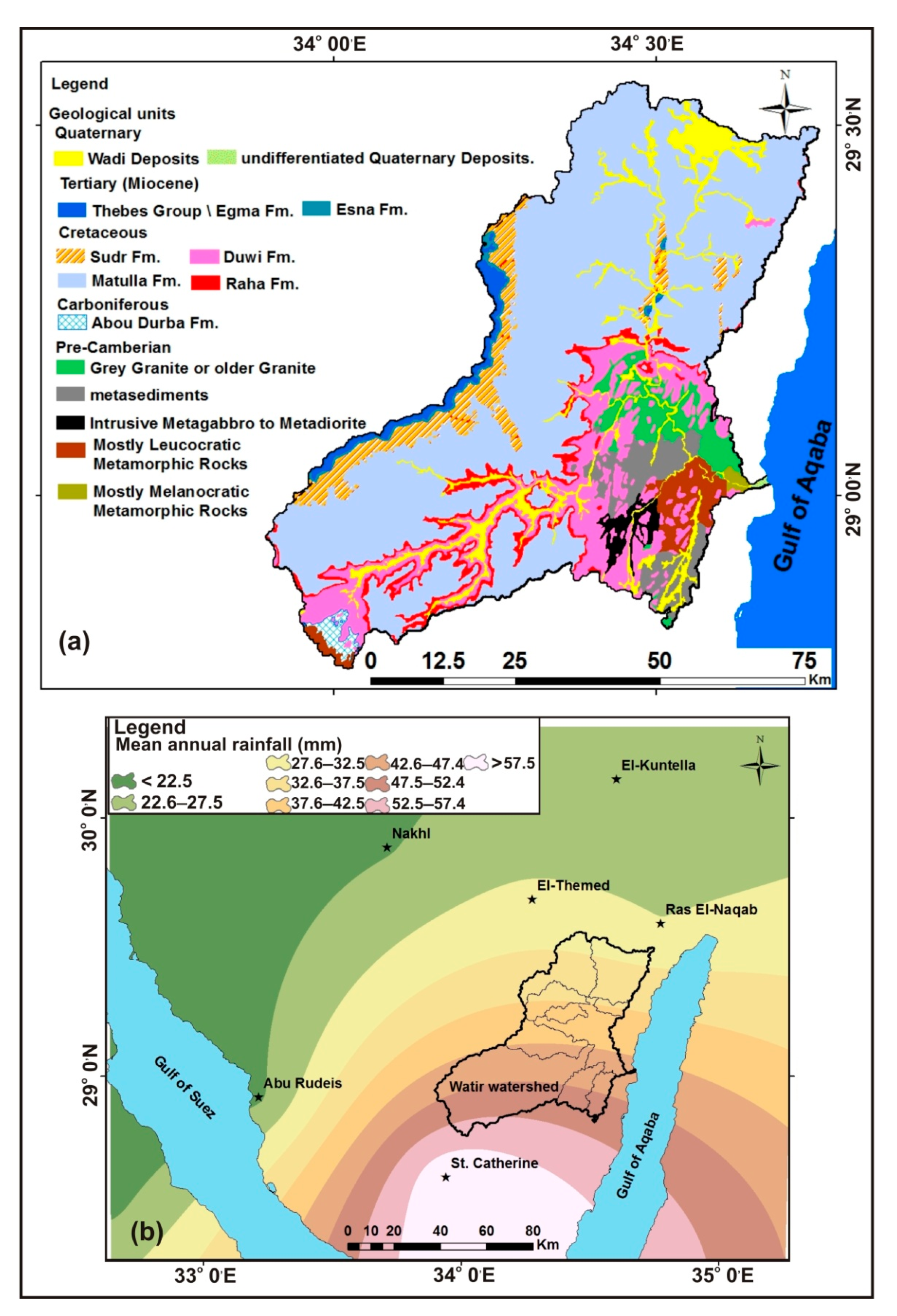
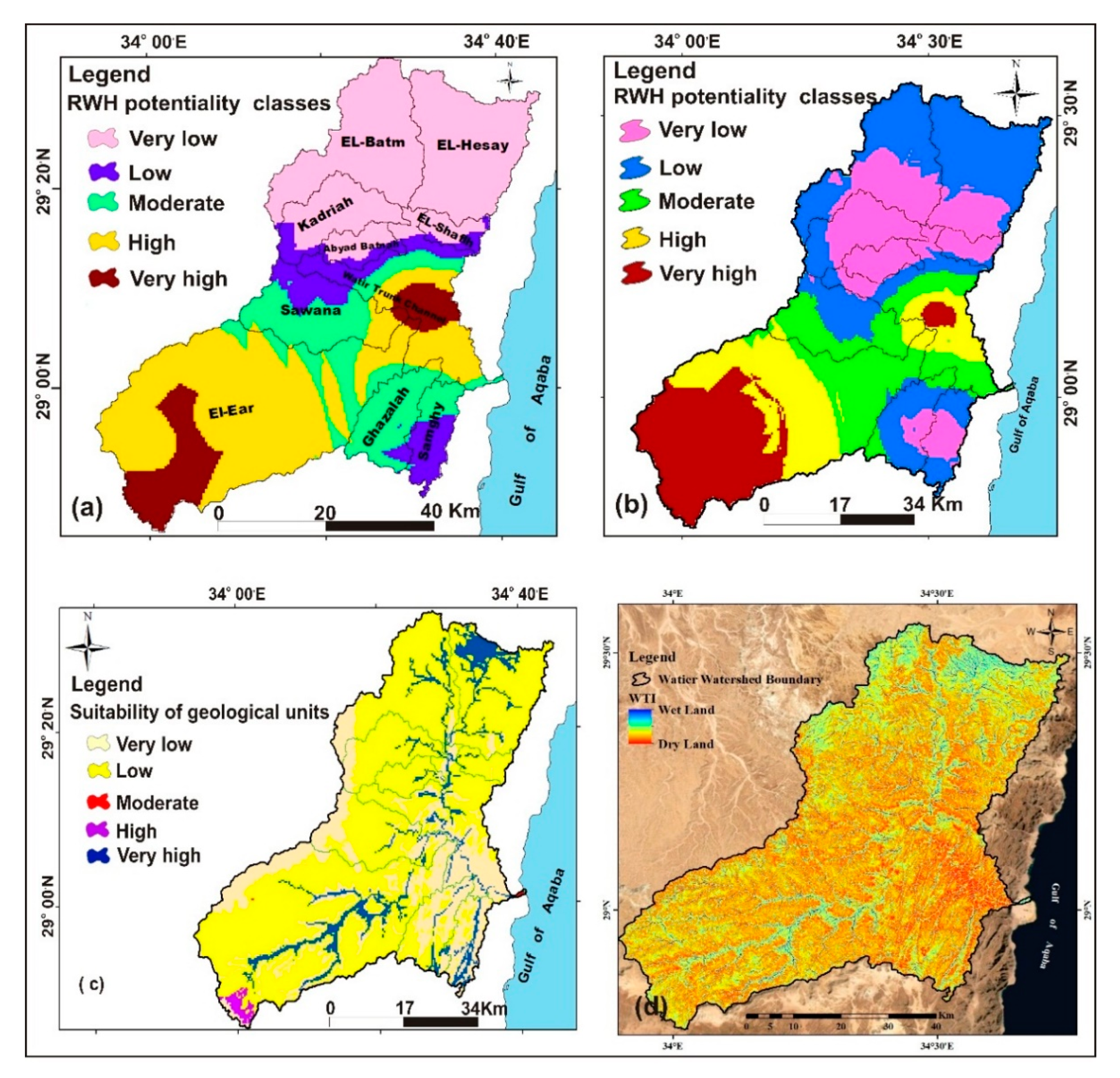
2.2. Geological Conditions

The geological map of Wadi Watir was produced within the ArcGIS 10.1© software, based on the geological map produced by CONOCO [36] (Figure 3a) and validated by Spot-4 satellite images using the ERDAS Imagine 9.3© software (Leica Geosystems GIS and Mapping LLC) [37]. The geological setting of the watershed is influenced by igneous and metamorphic rocks, whose ages range from Precambrian to Quaternary [38]. The Precambrian basement rocks mainly consist of igneous and metamorphic rocks differentiated into gneisses, meta-gabbros, meta-sediments, intrusive meta-gabbros and older granites dissected by basic dikes, fractures, joints and fault zones. Precambrian rocks underlie about 34% of the watershed. A sedimentary sequence forms the rest of the region [18], with sedimentary rocks ranging from the Carboniferous to Quaternary ages. The Quaternary deposits, consisting of detrital products from various sedimentary, igneous or metamorphic rocks [39,40], are mainly composed of granular sands or coarse gravels and carbonate rocks integrated into a clay matrix [41]. The main channels take many forms. Braided channels appear in the northern parts, in areas of low surface gradient, and parallel channels across the area adjacent to the cliff of the El-Egma Plateau. Wadi bottom soil occurs as long narrow strips of land occupying the lower parts of the flood plains. The lower units in the wadi feature a moderate sloping surface. The slope and topographic maps of the Wadi Watir watershed were created using ArcGIS 10.1© software from the Advanced Space-Borne Thermal Emission and Reflection (ASTER) DEM with 30-meter precision. In the present work, an isohyetal map was constructed in raster format (point format) for the mean annual precipitation recorded in mm for six climate stations near the studied watershed for the period from 1998 to 2008 [42,43] (Figure 3b). Nevertheless, some predictions of precipitation were also based on linear and non-linear approaches using climate indices. In these cases, the models required prior statistical correlation and trend analysis [44,45,46].

2.3. Surface Runoff Calculations

Surface runoff was calculated by applying the Finkel method [30] and the Soil Conservation Service Curve Number method (SCS-CN) [29] using the WMS 8.0© software [28]. The two methods were used together for the purposes of verification and validation [5]. The Finkel method was previously applied to calculate surface runoff in areas of similar climatic conditions to the study area as Wadi Arba, the Sinai Peninsula and other desert areas of Egypt [5,16,47,48]. It consists of a simple formula determining the possibility of annual or seasonal precipitation [5]. The SCS-CN method is widely used by many authors and is a more useful method for determining rainfall–runoff relationships in watersheds, with or without rain gauges [49]. However, some researchers, e.g., [50,51,52] have highlighted some limitations in the use of the SCS-CNS method for runoff calculation. Some of these limitations are not applicable for the studied watershed, where W. Watir could be considered as a medium-sized watershed with an area of about 3515 km². The landscape in which it was produced has a limited geographic variation. The method depends mainly on the selection of initial abstraction (Ia) (infiltration, evaporation, and surface depression storage) and the potential maximum retention (S) expressed in terms of curve number (CN) [53], which are suitable for the studied watershed area that is characterized by no wide geographic or geomorphic variation. Accordingly, the two methods were applied here in tandem for validation and comparison purposes.

The factors for the Finkel method were calculated according to peak flood flow (Q_max)

$$Q_{\mathit{max}}=K_1{A}^{0.67}$$

(1)

where Q_max = peak flood flow, m³/s and annual volume of flooding (V) at 1000 m³

$$V=K_2{A}^{0.67}$$

(2)

where A is the watershed area in (km²), and (K₁ and K₂) are constants depending on the probability of rainfall occurrence.

The probability of rainfall occurrence through a given year (for K₁ and K₂ calculation) was taken as 10%, i.e., 1.58 and 26.5 for K₁ and K₂, respectively [5,16,30,47].

It is noted that the probability of rainfall occurrence of 10% was used because it is very appropriate and less optimistic, but suitable to the local climate conditions of the study area [5,16,47].

The SCS-CN method was used to determine the annual flood volume of the watershed. This method was created on the basis of the water balance equation and the equations of proportional equality, and the linear relationship between the potential maximum retention and initial abstraction [51] (Equations (3)–(7)).

Water balance equation:

$$P=I_a+F+Q$$

(3)

where the proportional relationship is defined as:

$$\frac{Q}{P-I_a}=\frac{F}{S}$$

(4)

$$I_a=\lambda S$$

(5)

where P is the total precipitation (mm); Ia is the initial abstraction; Q is the volume of direct runoff (direct surface runoff depth in mm); F is the cumulative infiltration excluding Ia; S is the maximum potential water abstraction by soil in (mm); and λ is the 0.2 (standard value) [53]. The maximum potential retention limit at surface runoff start, S, is stated in terms of the scale parameter CN, which can vary between 0 and 100, signifying either zero storage or 100% surface runoff. The curve number is dependent on the hydrologic condition, soil groups and land use [29,42]. The value of CN was derived from the tables of United States Department of Agriculture-Soil Conservation Service-Curve Number (USDA-SCS-CN) for watershed characteristics [29], Wadi Watir geological map and the classification of the infiltration capabilities of the exposed rocks in the Sinai Peninsula established by [42] (

Table 1. Major exposed rocks in Sinai according to their infiltration capabilities and groundwater potentiality [42].

Lithologic Group	Soil Hydrologic Group	Infiltration Rate mm/h	Groundwater Potentiality
Sand dunes, Nile silt, undifferentiated Quaternary deposits, wadi deposits, G. El-Ahmar Fm., stabilized sandstone, Naqus Fm.	A	>7.62 (High)	High to very high
Risan Aneisa Fm., Safa, Cairo-Suez Hgul Fm., Abu Aggag Fm., Lake Nasser, Duwi Fm., lower to middle Miocene deposits, Hammamat clastics, and Ranga Fm., Umm Mahara, calc-alkaline granitic rocks-tectonized	B	3.81–7.62 (Moderate)	Moderate
Matulla Fm., Pliocene deposits, undifferentiated Plio- Pleistocene deposits, Gharandal Group, metasediments, Qiseib Fm., Abou Durba Fm.	C	1.27–3.81 (Low)	Low
Sabkhas deposits, undifferentiated Thebes Group, medium-to-high-grade metamorphic rocks, Samalut Fm., Mokattam Group, Egma Fm., Sudr Fm., Esna Fm., Masajid Fm., Tertiary alkali olivine basalts, older granite or grey granite, Katherina volcanics, intrusive metagabbro to metadiorite, mostly leucocratic medium-to-high grade metamorphic rocks, ring complexes, Ras Malaab Group, intermediate to acid metavolcanics and metapyroclastics, gabbroic rocks, gneiss and magmatic gneiss, Quseir Fm., pink granite, Trachyte plugs and sheets.	D	<1.27 (Very low)	Very low

). Subsequently, the CN values for Wadi Watir sub-watersheds were calculated, then, the values were added to the WMS 8.0© software to complete the surface runoff calculations.

$$S=\frac{25,400}{CN}-254$$

(6)

The direct surface runoff, Q, can be stated as:

$$Q=\frac{{(P-I_a)}^2}{(P-I_a)+S}=\frac{{(P-0.2S)}^2}{P+0.8S}$$

(7)

where Equation (7) is valid for P ≥ Ia, Q = 0

The average annual precipitation values were derived from the created isohyetal map and used in runoff calculations. The hydro-morphometric parameters were determined using the WMS 8.0© and ArcGIS 10.1© software (Aquaveo LLC, U.S. Army Corps of Engineers, Engineer Research & Development Center and Esri, Redlands, CA, USA).

The watershed area and watershed length were determined according to [54], whereas stream order was applied based on the hierarchical rank method [55]. The total number and total length of all streams in the watershed were determined according to [56,57], respectively. The infiltration number (IF) was calculated as in Equation (8) [58].

IF = DD * Fs

(8)

where DD is the drainage density and Fs is the stream frequency.

The drainage density and stream frequency were calculated according to [59] Equations (9) and (10).

DD = Σ Lu/A

(9)

Fs = Σ Nu/A

(10)

where Lu is the total length of all stream orders (km); A is the watershed area (km²) and Nu is the total number of all streams in the watershed.

2.4. Analytical Hierarchy Process (AHP) Technique

The analytical hierarchy process (AHP) was used to determine the weights of each RWH parameter. This technique was applied using its algorithms within the Microsoft Excel software. It is one of the common methods of multi-parameter decision analysis and was first created by Saaty [21]. AHP is generally implemented in three main steps: hierarchy creation, priority check, and consistency check [22]. Relative weights were determined by applying a pairwise comparison matrix to a set of parameters, thus determining the degree of relevance of each parameter and relativity to each other [60]. The pairwise comparison matrix reduces the cognitive load to determine the relative importance of many parameters at once [61]. The weighting of each RWH parameter (Wi) was determined by taking the eigenvector matching to the largest eigenvalue of the matrix and then was followed by normalizing components summation to unity [61] (Equation (11)). The importance of each RWH parameter was determined according to the Saaty importance scale [21] (

Table 2. Analytical hierarchy process (AHP) pairwise comparison scales [21].

Importance	Degree of Preference	Explanation
1	Equal	Two activities contribute equally to the goal
3	Moderate	Experience and judgment slightly or moderately favor one activity over another
5	Strong	Experience and judgment strongly or fundamentally favor one activity over another
7	Very strong	One activity is strongly favored over another and its dominance appears in practice
9	Extreme	Evidence of a preference for one activity over another is the most assured possible
2,4,6,8	Intermediate values	Used to represent compromises between preferences in weights 1, 3, 5, 7, and 9
Reciprocal	Opposites	Used for inverse comparison

).

$${\displaystyle \sum _{i=1}^{n}Wi=1}$$

(11)

where (Wi) is the weight of each parameter.

A pairwise comparison matrix (matrix A) was created for n parameters (eight RWH parameters were determined) according to the Saaty scale ratio, in the form of (n * n) as in Equation (12) [62,63].

Matrix A = (aij), i, j = 1, 2, 3…... n

(12)

where, a_ij represents the elements (RWH parameters) of matrix A.

The pairwise matrix was created as a square matrix (diagonal arrangement for the eight specific RWH parameters). The scores for the parameters are given on one side of the diagonal, where the other side is represented by the reciprocal value of the given scores. The score 1 to 9 and interchange values were assigned according to the Saaty scale [21]. The score 9 was assigned to the most important factor in determining RWH, while the score 1/9 was given to the least important one (Table 2). The generated matrix A1 was then normalized to produce a new matrix (matrix B) in order to obtain the relative values of eigenvector values for each RWH parameter (parameter weights) (Equation (13)) [64,65].

Matrix B = (bij), i, j = 1, 2, 3…... n

(13)

where bij are the elements of matrix B and can be defined as in Equation (14) [62]

$$bij=aij/{\displaystyle \sum _{i=1}^{n}aij=1,2,3,\dots \dots ,n}$$

(14)

Finally, parameter weights (Wi) were calculated as shown in Equation (15).

$$Wi=\frac{{\displaystyle {\sum }_{j=1}^{n}bij}}{{\displaystyle {\sum }_{i=1}^n{\displaystyle {\sum }_{j=1}^{n}bij}}}i,j=1,2,3,\dots \dots ,n$$

(15)

2.5. Watershed Modeling

Eight parameters were selected for the multi-parametric decision spatial model (MPDSM) application and embedding; VAF, OFD, MFD, IF, DD, A, BS and BL. These parameters were provided for the sub-watersheds in Wadi Watir and linked to ArcGIS 10.1© software in a geographical database format to produce spatial thematic layers using the spatial analyst module [20]. The thematic layers were then used as multi-decision support layers to construct the MPDSM for the optimal positioning of the RWH potentialities. The MPDSM was then created to classify the watershed into five possible RWH grading categories. MPDSM was run in two scenarios: the first proposed that all parameters used had the same degree of effectiveness for determining RWH, since equal weights were assigned to all parameters; the second scenario was applied using weights calculated using the AHP technique. The overall flow diagram of the methodology is shown in Figure 4.

3. Results and Discussion

3.1. Parameters of Multi-Parametric Decision Spatial Model (MPDSM)

Our MPDSM was used to resolve a wide range of problems involving complex parameters across different levels, where overlap between parameters was common [27,66,67]. The probability mapping of RWH for the Wadi Watir watershed was performed with spatial integration of eight parameters, namely VAF, OFD, IF, BS, DD, A, BL and MFD. These parameters were selected because they are the most effective ones in determining RWH potentiality, and moreover these parameters have been used in many previous studies related to RWH and flooding potentialities, e.g., [5,15,17,18,68,69]. The following is a description of these parameters:

3.1.1. Overland Flow Distance

The OFD parameter is an important factor for RWH, where it is affected by variations in slope, relief, lithology and topography, which together control the resulting erosion caused by surface runoff [70]. This consists of water flowing over watershed slopes and then becoming concentrated into a definite stream channel [57]. Most of the Wadi Watir watershed is composed of low (0.4304–0.4481 km) and moderate (0.4482–0.4691 km) OFD categories, which cover almost all of the watershed area (

Table 3. Output parameters resulting from the WMS 8.0© software, used to characterize watershed characteristics.

Sub-Watershed	Volume of Annual Flood (VAF) (m3) Finkel Method	Volume of Annual Flood (m3) SCS-CN Method	Overland Flow Distance (OFD) (km)	Max. Flow Distance (MFD) (km)	Watershed Infiltration Number (IN)	Drainage Density (DD) (km−1)	Watershed Area (A) (km2)	Watershed Slope (BS)(m/m)	Watershed Length (BL) (km)
El-Ear	3,203,020	13,258,477.9	0.380	87.88	0.83	0.76	1282.16	0.150	63.7
Sawana	1,207,680	3,962,709.9	0.390	42.78	0.80	0.78	299.01	0.180	31.02
Abyad Batnah	513,160	991,064.7	0.358	24.84	0.69	0.72	83.65	0.153	16.06
Kadriah	918,300	2,058,670.8	0.383	38.77	0.76	0.77	198.96	0.128	25.13
El-Batm	1,527,650	3,544,434.9	0.392	50.01	0.82	0.78	424.64	0.082	28.22
El-Hesay	1,556,920	2,592,202.9	0.432	44.43	0.92	0.87	436.85	0.078	32.02
El-Shaflh	428,160	601,010.1	0.345	20.91	0.78	0.68	63.61	0.159	13.70
Watir Trunk Channel	1,504,030	4,274,581.05	0.774	68.35	0.71	0.72	414.88	0.216	43.81
Samghy	686,980	1,393,763.4	0.398	28.30	0.80	0.80	128.82	0.179	23.21
Ghazalah	866,680	1,844,572.5	0.394	31.08	0.77	0.78	182.43	0.214	25.46

and

Table 4. Parameter ranges used to configure the MPDSM.

Watershed RWH Parameter	Very High	High	Moderate	Low	Very Low
VAF (m3) (Finkel Method)	>2,840,800	2,027,301–2,840,800	1,414,301–2,027,300	1,025,201–1,414,300	<1,025,201
VAF (m3) (SCS-CN Method)	>13,493,937.28	9,449,250.89–13,493,937.28	5,343,281.36–944,9250.88	2,646,823.77–534,3281.357	<2,646,823.77
OFD (km)	>0.5111	0.4692–0.5111	0.4482–0.4691	0.4304–0.4481	<0.4304
MFD (km)	>77.17	65.22–77.17	52.85–65.21	43.71–52.84	<43.71
IF	>0.846	0.811–0.846	0.786–0.810	0.751–0.785	<0.751
DD (km−1)	>0.81	0.776–0.81	0.757–0.775	0.733–0.756	<0.733
A (km2)	>1149.1	850.13–1149.1	540.85–850.12	303.73–540.84	<303.73
BS (m/m)	>0.19150	0.16152–0.19150	0.129116–0.16151	0.094321–0.129115	<0.094321
BL (km)	>57.37	44.85–57.37	34.2–44.84	26.06–34.19	<26.06

; Figure 1 and Figure 5a). High (0.4692–0.5111 km) and very high (>0.5111) OFD categories are represented only by small portions of the Wadi Watir trunk channel, Sawana and El-Ear sub-watersheds in the south-eastern parts of Wadi Watir. The very low OFD class (<0.4304 km) is represented by small areas scattered over all sub-watersheds except for the Wadi Watir trunk channel (Figure 1 and Figure 5a). The increase in OFD is generally towards the watershed outlet.

3.1.2. Volume of Annual Flood

The amount of running water caused by rainfall events is an important factor for managing RWH in watersheds. Wadi Watir is characterized by many rapid flood events with catastrophic effects. The highest level was recorded eleven years ago in January 2010 [18]. Water runoff in Wadi Watir was increased by surplus water flowing across broken rocks and down the valleys. The watershed is classified into five VAF categories (Figure 5b,c; Table 4). It should be noted that there is a high degree of correspondence between the two resulting VAF maps [29,30], where the high and very high VAF classes are made up of most of the south-western part of the watershed. The El-Ear sub-watershed has the largest area among all Wadi Watir sub-watersheds, with a sixth-order trunk channel and an average watershed slope of 0.15 m/m. It receives the highest VAF value among the Wadi Watir sub-watersheds (Table 3; Figure 1). Low, very low and moderate VAF classes consist of the central and eastern parts of Wadi Watir sub-watersheds.

3.1.3. Watershed Slope

BS is an effective factor in determining rainwater acceleration, infiltration capability, runoff potentialities and optimum locations for water harvesting [42,71,72]. Usually, the higher the runoff related to steeper watershed slopes, the higher the potentiality for flooding [5,18,73]. The resulting slope map shows five categories ranging from gentle to steep slopes (Figure 5d). The thematic layer for BS indicates a linear increase in slope values from the north-eastern and south-western parts towards the eastern parts at the outlet of the watershed (Figure 5d). Steep slopes (0.16152–0.19150 m/m) and very steep slopes (>0.19150 m/m) are mainly present in the Samghy and Ghazalah sub-watersheds as well as relatively large areas of the Wadi Watir trunk channel, and Sawana and El-Ear sub-watersheds. BS decreases towards the upstream parts of Wadi Watir in the northern and north-eastern parts, which feature mostly gentle slopes (<0.094321 m/m) (Figure 5d).

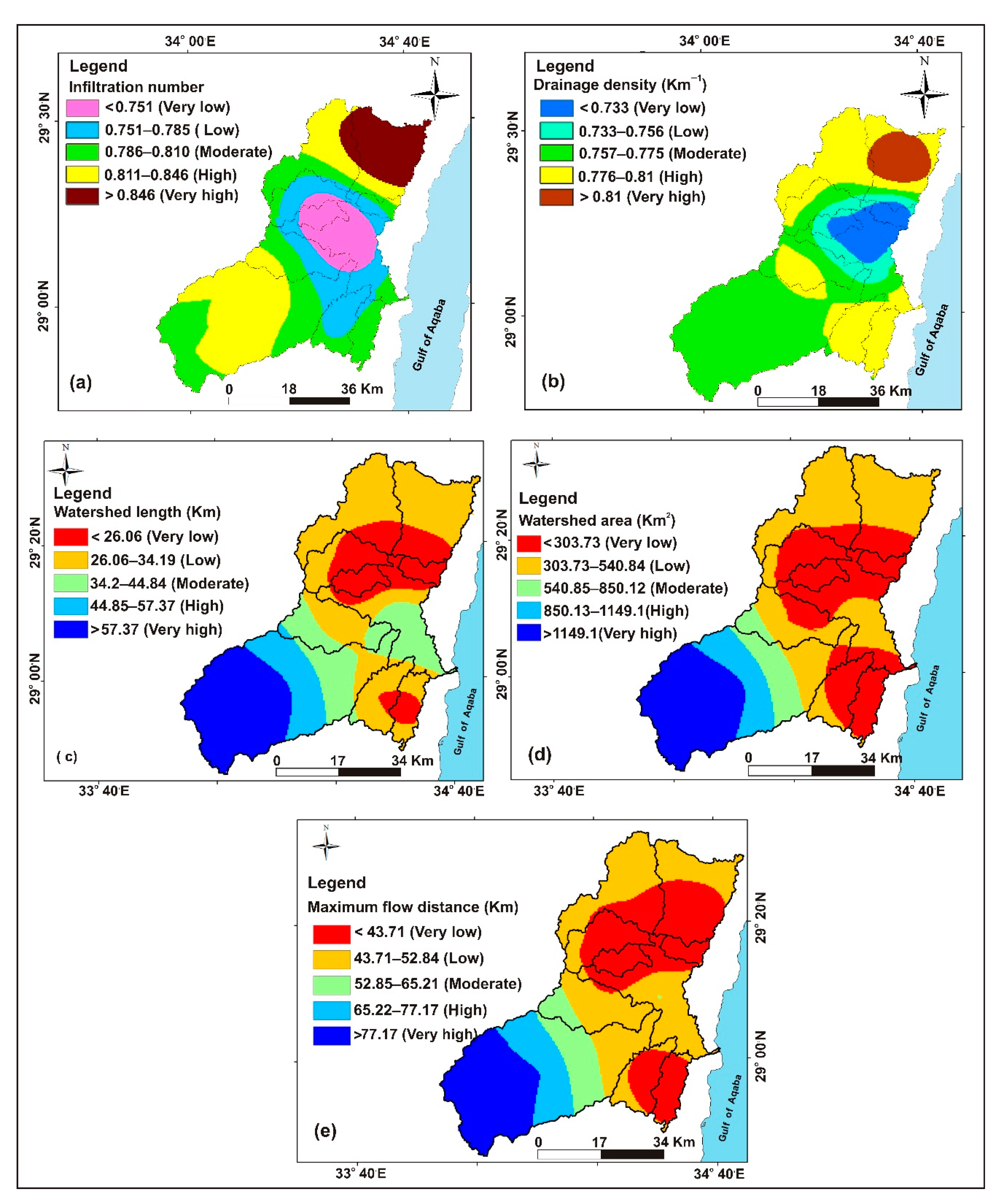
3.1.4. Infiltration Number

IF is a controlling factor for RWH specification, where it is based on drainage density and stream frequency. It is an important factor for understanding the infiltration potentiality of watersheds. The higher the infiltration number, the lower the actual infiltration, and hence the higher the runoff [74]. This leads to higher DD. The IF map shows that the major area of the watershed is represented by high to moderate IF categories which reflect the moderate infiltration capability of its soil types (Figure 6a; Table 4). Moderate, high and very high IF categories represent most of the Wadi Watir trunk channel and small parts of El-Ear, Sawana and Ghazalah sub-watersheds. Very low and low IF classes make up the central and south-eastern parts of the Wadi Watir watershed, which consist of most of the Wadi Watir trunk channel, Ghazalah, Abyad Batnah, Kadriah and small portions of the El-Ear, Sawana and El Batam sub-watersheds (Figure 6a). The north-eastern corner of the watershed (most parts of El-Hesay and small parts of El-Batam sub-watersheds) features in the very high IF class.

3.1.5. Drainage Density

High DD is an important factor for rapid floods and high runoff volumes [75,76]. Consequently, it is an important factor for RWH potentiality determination. The spatial distribution of the DD classes decreases from very high to very low categories (Figure 6b). The thematic layer for DD indicates that the very high DD category (>0.81 km⁻¹) is made up of a small portion of the north-eastern side of Wadi Watir (El-Hesay sub-watershed). Most of the northern parts of Wadi Watir and the south-eastern corner, which includes most of the Samghy and Ghazalah sub-watersheds, are characterized by high DD values (Figure 6b). Most of the Wadi Watir watershed area features moderate DD. The low and extremely low DD categories represent small portions of the central and eastern parts of the watershed (most portions of the Abyad Batnah, Shaflah and Wadi Watir trunk channel sub-watersheds). In general, the DD values for Wadi Watir sub-watersheds are moderate and close together, with an average value of 0.76 km⁻¹, indicating moderate permeability for the watershed subsoil [77]. These values reflect moderate potential for recharging groundwater by applying the appropriate RWH systems. The value of DD increases as a result of impermeable and weak subsurface material and mountainous relief. Low drainage density results in coarse drainage texture and highly permeable subsoil, while high DD leads to fine drainage texture with poorly permeable sub-soil and impervious basal rocks [78].

3.1.6. Watershed Length

BL is one the most controlling factors for RWH determinations, which is because the longer the watershed, the lower its slope, and therefore the greater the possibilities of RWH [5]. The thematic layer for BL is classified into five categories from very low to very high (Figure 6c). High (44.85–57.37 km) and very high (>57.37 km) BL categories represent only some parts of El-Ear and a very small portion of the Sawana sub-watershed on the south-western side of the Wadi Watir watershed. Most of the Wadi Watir sub-watersheds are in low to very low BL categories (less than 34.19 km). The moderate BL class (34.2–44.84 km) represents some parts of the Wadi Watir trunk channel, Ghazalah, El-Ear and Sawana sub-watersheds (Figure 6c). The largest BL value was observed in the El-Ear sub-watershed, which had the highest watershed area value, indicating higher potential for RWH [5], while the smallest BL value was observed in the El-Shaflh sub-watershed, which had the lowest watershed area value (Table 3).

3.1.7. Watershed Area

Watershed area is one of the most important factors in determining RWH potential, as it significantly affects the watershed runoff processes. The greater the area of the watershed, the greater the volume of rain collected and the higher the peak flood discharge [79,80]. The reclassified map for the watershed area reflects a discrepancy in the regions between the different sub-watersheds from very low to very high (Figure 6d). The regions with a very high (>1149.1 km²) and high (850.13–1149.1 km²) watershed area occur mainly in the south-western parts of the watershed, where most parts of the El-Ear sub-watershed are included in this class, which also have higher values of VAF, BL, and MFD, indicating high potentiality for RWH [81]. The moderate watershed area class (540.85–850.12 km²) is represented only by a small strip of the El-Ear and Sawana sub-watersheds. Most of the Wadi Watir watershed is represented by low to very low watershed area classes, which generally extend from the central parts to the eastern and north-eastern sides of the watershed (Figure 6d).

3.1.8. Maximum Flow Distance

The watershed maximum flow distance (MFD) includes both channel and overland flows [57]. MFD is a vital factor in determining RWH potential in watersheds, and higher RWH potentiality in a watershed is related to higher values of MFD [5]. These values generally increase toward the south-western side of the watershed (Figure 6e). High (65.22–77.17 km) and very high (>77.17 km) MFD classes represent large areas of the El-Ear sub-watershed, which also have the highest A and BL values. The moderate class (52.85–65.21 km) consists only of a small strip in the sub-watersheds of the El-Ear and Sawana. The remaining parts of the watershed feature in the extremely low MFD classes (Figure 6e).

3.2. Multi-Parametric Decision Spatial Model

The MPDSM of Wadi Watir was implemented using two scenarios with equal weights for all parameters and weights determined by AHP. This model is a good example of the distributed model of hydrology, as it relies on the spatial variance of a set of effective parameters to determine RWH potential.

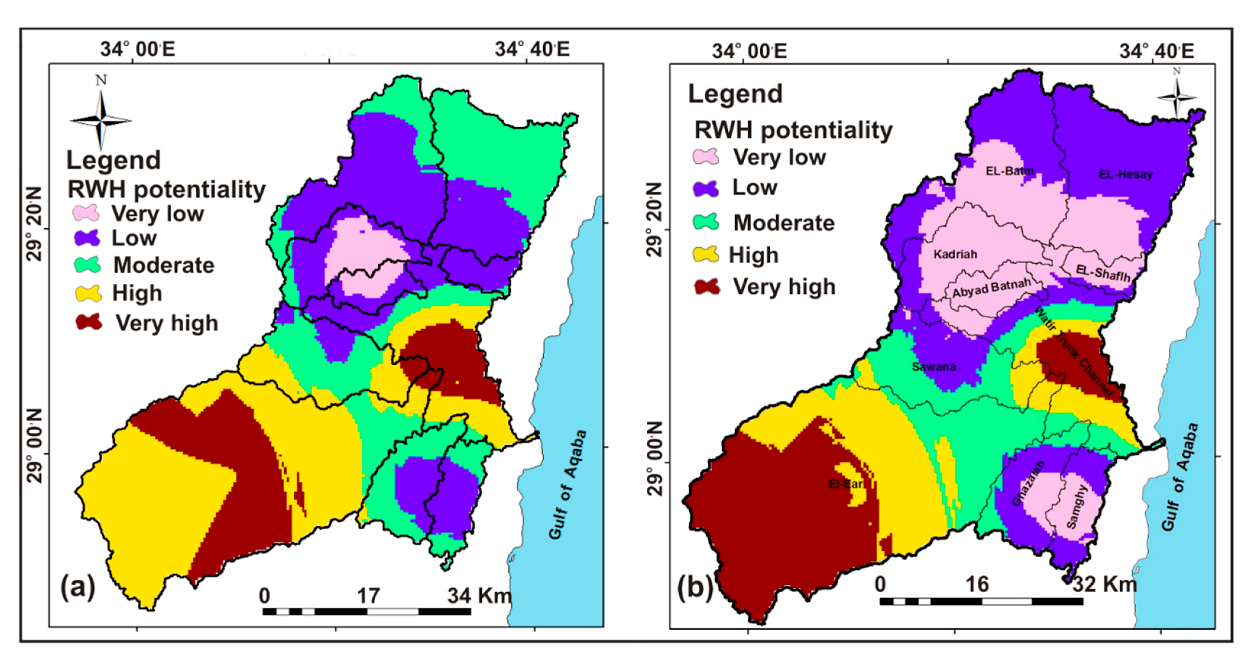
3.2.1. Multi-Parametric Decision Spatial Model Scenario I

In this scenario, rates and weights were determined according to the magnitude of contributions, comparing each layer range of the MPDSM, where the equal weight for each parameter was set as 12.5%. Each parameter was categorized into five categories from very low to very high probability according to the size of its contribution in determining the RWH potential (

Table 5. Basic case scenario I for MPDSM (equal weights to parameters), ranks, weights and degree of effectiveness of parameters used in mapping RWH potentialities.

Thematic Layers (Parameter)	Probability Category for RWH	Class Rank (%)	Average Rate (Rank) (CR) %	Weight % (CW)	Degree of Effectiveness (DE)
Average overland flow distance (OFD)	I (Very high) II (High) III (Moderate) IV (Low) V (Very low)	100–80 80–60 60–40 40–20 20–0	0.9 0.7 0.5 0.3 0.1	12.5	11.25 8.75 6.25 3.75 1.25
Volume of annual flood (VAF)	I (Very high) II (High) III (Moderate) IV (Low) V (Very low)	100–80 80–60 60–40 40–20 20–0	0.9 0.7 0.5 0.3 0.1	12.5	11.25 8.75 6.25 3.75 1.25
Infiltration number (IF)	I (Very high) II (High) III (Moderate) IV (Low) V (Very low)	100–80 80–60 60–40 40–20 20–0	0.9 0.7 0.5 0.3 0.1	12.5	11.25 8.75 6.25 3.75 1.25
Maximum Flow distance (MFD)	I (Very high) II (High) III (Moderate) IV (Low) V (Very low)	100–80 80–60 60–40 40–20 20–0	0.9 0.7 0.5 0.3 0.1	12.5	11.25 8.75 6.25 3.75 1.25
Drainage density (DD)	I (Very high) II (High) III (Moderate) IV (Low) V (Very low) V (Very low)	100–80 80–60 60–40 40–20 20–0	0.9 0.7 0.5 0.3 0.1	12.5	11.25 8.75 6.25 3.75 1.25
Watershed area (A)	I (Very high) II (High) III (Moderate) IV (Low) V (Very low)	100–80 80–60 60–40 40–20 20–0	0.9 0.7 0.5 0.3 0.1	12.5	11.25 8.75 6.25 3.75 1.25
Watershed length (BL)	I (Very high) II (High) III (Moderate) IV (Low) V (Very low)	100–80 80–60 60–40 40–20 20–0	0.9 0.7 0.5 0.3 0.1	12.5	11.25 8.75 6.25 3.75 1.25
Watershed slope (BS)	I (Very high) II (High) III (Moderate) IV (Low) V (Very low)	100–80 80–60 60–40 40–20 20–0	0.9 0.7 0.5 0.3 0.1	12.5	11.25 8.75 6.25 3.75 1.25

). Assuming that the total value of the ranks of all categories equals 100%, the ranks of the five categories will be classified as 0–20% (very low), 20–40% (low), 40–60% (moderate), 60–80% (high) and 80–100% (very high), respectively. The degree of effectiveness (DE) was estimated for each thematic layer by multiplying the rank of the parameter (CR) by the weight of the parameter (CW) [42] (Equation (16)) (Table 5).

$$DE=CWxCR$$

(16)

In this way of analyzing and processing data, the degree of effectiveness of each parameter provides a relative comparison between the different thematic layers. Accordingly, category V for all parameters has a DE value of 1.25, so it is the least effective category in mapping RWH potentialities, whereas category I (DE = 11.25) is the most effective category (Table 5).

Our MPDSM was created by incorporating the eight thematic layers using a weighted overlay spatial analyst model within the ArcGIS 10.1© software. The MPDSM model was run twice; one with the VAF calculated using the SCS-CN and the other using the Finkel surface runoff method. Two maps of RWH potentialities were produced from the operation of this model, as each map contained five RWH potentiality categories, ranging from very low to very high (Figure 7;

Table 6. Areas with RWH potential categories resulting from first model scenario.

Areas with Categories of RWH Potential; VAF Calculated Using the Finkel Method [30]
RWH Potentiality Class	Very Low	Low	Moderate	High	Very High
Area (km2)	301.17	1298.35	932.13	501.03	480.35
Area (% of total watershed area) Total watershed area 3513 Km2	8.57	36.95	26.53	14.26	13.67
Areas with Categories of RWH Potential; VAF Calculated Using the SCS-CN Method [29]
RWH Potentiality Class	Very Low	Low	Moderate	High	Very High
Area (km2)	845.19	855.54	736.98	534.27	541.07
Area (% of total watershed area) Total watershed area 3513 Km2	24.05	24.35	20.97	15.2	15.4

). The maps show the spatial distribution of these categories in relation to the total watershed area (Table 6). There is a very good match between the two maps produced from the first scenario, where the high and very high RWH potential categories make up the south-western and some of the south-eastern areas of Wadi Watir. These categories represent most of the El-Ear and the main trunk channel sub-watersheds as well as small parts of the Sawana sub-watershed. The moderate RWH potential class is distributed over the central and south-eastern regions as well as some northern regions, according to the Finkel RWH potentiality map (Figure 7).

3.2.2. Multi-Parametric Decision Spatial Model Scenario II (Weights Assigned by the AHP Technique)

A second MPDSM scenario was created using weights defined by means of the AHP method [21]. This method relies on expert judgment to determine the relative importance among the eight RWH parameters. To achieve greater accuracy in determining the relationship and significance between the parameters, bivariate correlations were made using the Pearson correlation coefficient “r” in SPSS Software version 25 (SPSS Inc., Chicago, IL, USA) [82] (

Table 7. Correlation matrix of studied model parameters using the Pearson correlation.

Parameter	VAF (Finkel Method)	VAF (SCS-CN Method)	OFD	MFD	IF	DD	A	BS	BL
VAF (Finkel method)	1
VAF (SCS-CN method)	0.960 **	1
OFD	0.167	0.091	1
MFD	0.943 **	0.908 **	0.451	1
IF	0.427	0.259	−0.290	0.201	1
DD	0.241	0.048	−0.130	0.088	0.762 *	1
A	0.990 **	0.980 **	0.097	0.917 **	0.389	0.164	1
BS	−0.198	−0.025	0.392	−0.033	−0.616	−0.457	−0.169	1
BL	0.956 **	0.942 **	0.375	0.974 **	0.261	0.161	0.942 **	0.055	1

** Correlation significant at 0.01 level (2-tailed). * Correlation significant at 0.05 level (2-tailed).

). The best way to present the value of “r” is to square it to “r²”. It is a value from zero to one, and it is the fraction of the variance between two variables which are “shared”. Correlations between VAF, MFD, A and BL are high, and their coefficients are important (r² > 0.9). There are other important correlations between A and BL (r² = 0.9), and there are other strong positive correlations between MFD, BL and A (r² > 0.9). High correlation was also observed between IF and DD (r² > 0.7). Accordingly, there are strong relationships between the parameters chosen for MPDSM application, some of which positively affect the RWH capability, namely VAF, A, MFD, IF, DD, OFD and BL, while others such as BS have a negative effect [5]. The pairwise comparison matrix was used to determine the importance of the model parameters in relation to each other (

Table 8. Pairwise comparison matrix (matrix A) for parameters used in determining RWH potentiality.

Parameter	VAF	OFD	MFD	IF	Dd	A	BS	BL
VAF	1	9	5	3	5	1	1	7
OFD	1/9	1	1/3	1/3	1/3	1/9	1/9	1/3
MFD	1/5	3	1	3	3	1/3	1/3	1
IF	1/3	3	1/3	1	1	1/3	1/5	3
Dd	1/5	3	1/3	1	1	1/9	1/7	1/3
BA	1	9	3	3	9	1	1	5
BS	1	9	3	5	7	1	1	7
BL	1/7	3	1	1/3	3	1/5	1/7	1
SUM	3.98	40.06	14	16.66	29.33	4.08	3.93	24.66

and

Table 9. Normalized matrix (matrix B).

Parameter	VAF	OFD	MFD	IF	DD	A	BS	BL	Eigen-Values (Weights)	Weight%	Consistency
VAF	0.251	0.225	0.357	0.180	0.170	0.245	0.254	0.284	0.246	24.574	8.690
OFD	0.028	0.025	0.024	0.020	0.011	0.027	0.028	0.014	0.022	2.208	8.380
MFD	0.050	0.075	0.071	0.180	0.102	0.082	0.085	0.041	0.086	8.571	8.592
IF	0.084	0.076	0.024	0.060	0.034	0.082	0.051	0.122	0.066	6.640	8.641
DD	0.050	0.076	0.024	0.060	0.034	0.027	0.036	0.014	0.040	4.009	8.257
A	0.251	0.225	0.214	0.180	0.307	0.245	0.254	0.203	0.235	23.479	8.589
BS	0.251	0.225	0.214	0.300	0.239	0.245	0.254	0.284	0.251	25.141	8.659
BL	0.036	0.075	0.071	0.020	0.102	0.049	0.036	0.041	0.054	5.378	8.667
	1	1	1	1	1	1	1	1	1		λ max = 8.69
											CI = (0.099)
											RI = 1.41
											CR = 0.069

).

The large number of parameters, so-called over-parameterization, is a real problem in hydrological models, especially in distributive models [83]. Optimal assessment of the likelihood of harvesting runoff water requires correct estimates of the weights of all elements in the model to determine the priority areas. AHP is a designed technique proposed by Saaty [21,60] for analyzing complex decisions taking into consideration a large number of factors. Accordingly, we eliminated the drawbacks of over-parameterization in the model by applying AHP to adjust the weights in the multi-parametric spatial model. Weights were assigned to each RWH parameter after systematic pairwise comparisons based on expert judgment. Then new weights were obtained for the final eight parameters and distributed as 24.57, 23.47, 2.2, 8.57, 6.64, 4.009, 25.14 and 5.37 for VAF, A, OFD, MFD, IF, DD, BS and BL respectively (Table 9). Based on the AHP weights for each thematic layer, a new multi-layer computational overlay was built into the ArcGIS 10.1© spatial analyst model builder. RWH maps were obtained, showing five classes ranging from very high to very low (Figure 8). These maps indicate that very high and high probability classes are the most appropriate places to harvest flood water. These classes make up most of the south-western, south-eastern and central parts of the watershed, representing about 33.24% of the total watershed area (

Table 10. Areas with categories of RWH potential in Wadi Watir watershed resulting from the MPDSM second scenario.

Areas with Categories of RWH Potential; VAF Calculated Using the Finkel Method [30]
RWH Potentiality Class	Very Low	Low	Moderate	High	Very High
Area (km2)	1161.1	320.59	616.77	1110.72	303.83
Area (% of total watershed area) Total watershed area 3513.01 km2	33.05	9.12	17.55	31.61	8.64
Areas with Categories of RWH Potential; VAF Calculated Using the SCS-CN Method [29]
RWH Potentiality Class	Very Low	Low	Moderate	High	Very High
Area (km2)	801.48	936.08	607.85	555.27	612.33
Area (% of total watershed area) Total watershed area 3513.01 km2	22.81	26.65	17.30	15.81	17.43

). Other parts of the watershed rank low for potential flood water harvesting. There is a significant match in the results between the two model scenarios, which reflects the high credibility of these results, and their suitability for application elsewhere in similar arid regions.

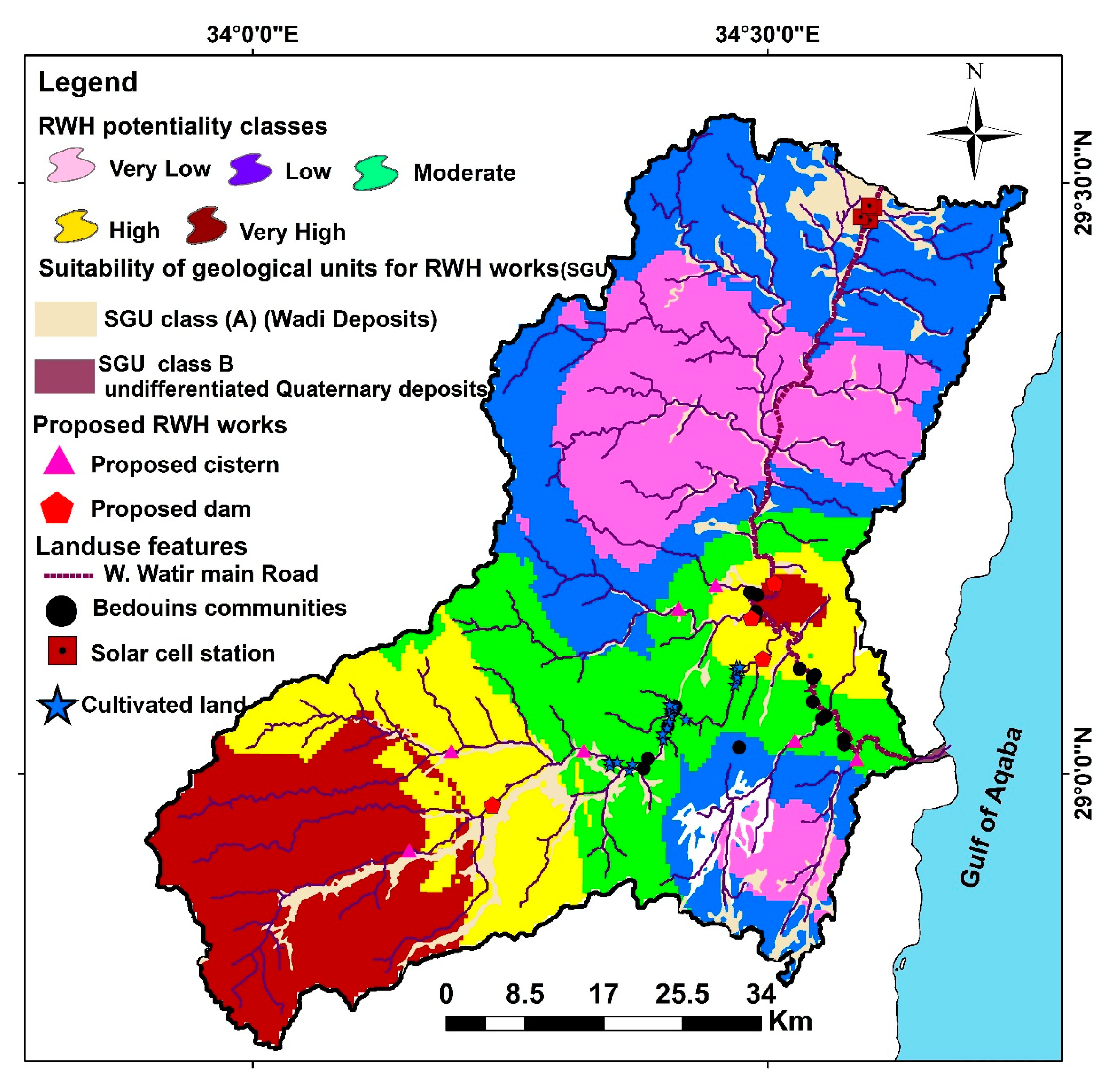
3.3. Model Validation and Justification

Weights from the AHP technique must be examined to determine their consistency. Accordingly, the consistency ratio (CR) and consistency index (CI) were calculated for the weights specified for the eight RWH parameters. This examination method is one of the strengths of AHP [62,63]. CR is used as an indication of the probability that the placings in the generated matrix were randomly generated [60,84,85], and it works by comparing the consistency index to the random index (Equations (17) and (18)) [60].

$$CR=\frac{CI}{RI}$$

(17)

$$CI=\frac{(\lambda \mathit{max}-n)}{n-1}$$

(18)

where λ max signifies the largest eigenvalue in the matrix; n is the order of the matrix (number of used parameters) and RI is the random index derived from [60], and it amounted to 1.41 in the case of the eight parameters.

According to [60], CR ˂ 0.1 indicates acceptable consistency for the applied pairwise comparison matrix and the determined weights are valid for model application. CR ≥ 0.1 means that the array values need to be modified and adjusted. The CR value for the matrix created in the current work was 0.069, indicating consistency and usability (Table 9). To categorize the advantages of the model results, areas with high to very high potential for flood water harvesting can be equipped with harvesting facilities, in the form of ground cisterns or dams with reservoirs.

In this regard, it is important to determine the suitability of geological units for the establishment of flood water collection facilities, with a map of five categories ranging from very low to very high potential (Figure 8c). The very high potential category (class A) is made up of wadi sediments in the main trunk channels. The high potential category (class B) consists of undifferentiated Quaternary sediments, which are mainly exposed in the part of the main tributaries of the watershed near the exit into the Gulf of Aqaba. These two classes represent the Quaternary soil type [18]. Areas with these categories are most suitable for establishing floodwater harvesting facilities, limited agricultural activities using harvested water, as well as natural recharge of the underlying aquifer. On the other hand, the moderate, low and very low potential categories (classes C, D and E, respectively) are characterized by types of geological units unsuitable for constructing floodwater collection facilities, such as fractured limestone and igneous rocks (Figure 8c). These units were classified as clastic rock soil, carbonate rock soil and basement rock soil for classes C, D, and E, respectively [18]. Additionally, to verify the accuracy of the model results, a topographic wetness index (TWI) for Wadi Watir was determined using DEM within the ArcGIS 10.1© software based on the formula [86]

$$TWI=lin(\frac{A}{\tan \beta })$$

(19)

where A is the watershed area and β is the local slope.

The watershed area encloses sites which are capable of receiving water from the sloping land, and the local slope has the ability to make water flow [87,88]. The TWI is an effective method for determining humidity in watersheds [89,90,91]. High TWI values indicate high potential for runoff concentration [70]. The resulting TWI map of Wadi Watir watershed shows variation in TWI grades from wet to arid (Figure 8d). Higher TWI grades (shown in blue) appear mainly in the main trunk channels, indicating high flood potential and higher potential for RWH at specific sites to establish RWH structures (Figure 8d and Figure 9). On this basis, four dams were proposed to harvest flood water in areas featuring RWH potential classes A and B to mitigate the risk of sudden floods, improve the natural recharge of aquifers and store large quantities of water for population use (Figure 9). It was also proposed to create seven groundwater cisterns to conserve water for use in dry seasons, for limited agricultural activities and drinking water supplies for people and animals. The proposed facilities take into account aspects of the current land use including roads, communities and cultivated land (Figure 9 and Figure 10), whereby the Wadi Watir watershed is characterized by natural desert landscape and vegetation with poor coverage taking up more than 30% of the ground area [18].

4. Conclusions

RS, GIS, WMS and AHP are techniques which have proved to be very effective in optimum RWH site determination. These techniques were integrated to construct a multi-parametric decision spatial model to identify potential sites for RWH in the Wadi Watir watershed on the Sinai Peninsula. A digital elevation model, Landsat ETM ⁺ satellite images, topographic maps and precipitation data were used as the basic dataset within the ArcGIS 10.1© and WMS 8.0© software to define the watershed morphometric and hydrological parameters. Eight hydro-morphometric parameters were used, namely the volume of annual flood, watershed infiltration number, maximum flow distance, watershed slope, watershed area, watershed length, drainage density and overland flow distance. These parameters were used as thematic layers to build a multi-parametric spatial model, and were assigned weights and ranks according to their effect on RWH potentiality mapping. The model run started with assuming equal weights for all parameters, and then an analytical hierarchy process (AHP) was applied to adjust the model parameter weights. Furthermore, the consistency ratio (CR) was calculated to validate the applied model, producing a value less than 0.1 (0.069), indicating that the applied model was appropriate. Subsequently, a justified multi-parametric decision spatial model was developed for the Wadi Watir watershed in southern Sinai, which separated it into five classes of RWH potential, ranging from very high to very low. Low, very low and moderate RWH classes represented 26.65%, 22.81% and 17.3% of the total watershed area, respectively. The areas consisting of high and very high classes were chosen as the most suitable sites for installing RWH structures, and they account for 33.24% of the total watershed area. These areas occupy most of the south-western, south-eastern and central parts of the watershed. The current work proposes appropriate RWH structures to be applied in these locations, represented by four retention dams and seven groundwater storage cisterns. These measures will reduce the risk of sudden floods, enhance soil moisture, replenish groundwater reserves and raise the living standards for local residents. Current land-use features and soil characteristics were used to identify the proposed sites for the implementation RWH facilities.

The accuracy of the model results was checked using a watershed topographic wetness index (TWI) map. This map confirmed that the proposed RWH structures were selected in areas of higher TWI classes represented by higher soil permeability in Wadi sediments and undifferentiated Quaternary deposits. The study concluded that the RWH potentiality in Wadi Watir watershed exists, which could open opportunities for the maximization of water availability and sustainable development. With regard to the future work plan, the current research presupposes additional future studies, including complete site characterization and detailed field surveying of the proposed RWH sites, compilation and analysis of previous and ongoing RWH activities, evaluation and monitoring of surface flooding operations, and coordination of activities with various owners, local authorities and Bedouins, identifying suitable types of RWH dams, cistern designs and storage capabilities.

References

1. Foody, G.M.; Ghoneim, E.M.; Arnell, N.W. Predicting locations sensitive to flash flooding in an arid environment. J. Hydrol. 2004, 292, 48–58. [Google Scholar] [CrossRef]
2. Hardy, J.; Gourley, J.J.; Kirstetter, P.E.; Hong, Y.; Kong, F.; Flamig, Z.L. A method for probabilistic flash flood forecasting. J. Hydrol. 2016, 541, 480–494. [Google Scholar] [CrossRef] [Green Version]
3. Berghuijs, W.R.; Woods, R.A.; Hutton, C.J.; Sivapalan, M. Dominant flood generating mechanisms across the United States. Geophys. Res. Lett. 2016, 43, 4382–4390. [Google Scholar] [CrossRef] [Green Version]
4. Kousky, C.; Michel-Kerjan, E. Examining flood insurance claims in the United States: Six key findings. J. Risk Insur. 2017, 84, 819–850. [Google Scholar] [CrossRef]
5. Elewa, H.H.; Qaddah, A.A.; El-Feel, A.A. Determining potential sites for runoff water harvesting using remote sensing and geographic information systems-Based Modeling in Sinai. Am. J. Environ. Sci. 2012, 8, 42–55. [Google Scholar]
6. Pallard, B.; Castellarin, A.; Montanar, A.A. Look at the links between drainage density and flood statistics. Hydrol. Earth Syst. Sci. 2009, 13, 1019–1029. [Google Scholar] [CrossRef] [Green Version]
7. Asadi, A. The comparison of lumped and distributed models for estimating flood hydrograph (Study Area: Kabkian Basin). J. Electron. Comm. Eng. Res. 2013, 1, 7–13. [Google Scholar]
8. Refsgaard, J.C.; Knudsen, J. Operational validation and Intercomparison of different types of hydrological models. Water Resour. Res. 1997, 32, 2189–2202. [Google Scholar] [CrossRef]
9. Smith, M.B.; Seo, J.; Koren, V.; Reed, M.; Zhang, Z.; Duan, Y.; Moreda, F.; Cong, S. The distributed model intercomparison project (DMIP): Motivation and experiment design. J. Hydrol. 2004, 298, 4–26. [Google Scholar] [CrossRef]
10. Vieux, B.E.; Cui, Z.; Gaur, A. Evaluation of a Physics-based distributed hydrologic model for flood forecasting. J. Hydrol. 2004, 298, 155–177. [Google Scholar] [CrossRef]
11. Bicknell, B.; Imhoff, J.; Kittle, J.; Donigian, A.; Johanson, R. Hydrological Simulation Program-FORTRAN, User’s Manual for Version 11; Environmental Protection Agency (EPA): Washington, DC, USA, 1997; p. 770. [Google Scholar]
12. Bobba, A.G.; Singh, V.P.; Bengtsson, L. Application of environmental models to different hydrological systems. Ecol. Model. 2000, 125, 15–49. [Google Scholar] [CrossRef]
13. Vazquez, R.F.; Feyen, L.; Feyen, J.; Refsgaard, J.C. Effect of grid size on effective parameters and model performance of the MIKE-SHE code. Hydrol. Process. 2002, 16, 4–18. [Google Scholar] [CrossRef]
14. Murari, P.; Nelson, E.J.; Downer, W. Assessing the capability of a distributed and a lumped hydrologic model on analyzing the effects of land use change. J. Hydroinform. 2010, 18, 65–80. [Google Scholar]
15. Lin, K.; Chen, H.; Xu, C.; Yan, P.; Lan, T.; Liu, Z.; Dong, C. Assessment of flash flood risk based on improved analytic hierarchy process method and integrated maximum likelihood clustering algorithm. J. Hydrol. 2020, 584, 124696. [Google Scholar] [CrossRef]
16. Elewa, H.H.; Ramadan, E.M.; Nosair, A.M. Water/Land Use planning of Wadi El-Arish watershed, Central Sinai, Egypt using RS, GIS and WMS techniques. Int. J. Sci. Eng. Res. 2014, 5, 341–349. [Google Scholar]
17. Elewa, H.H.; Ramadan, E.M.; Nosair, A.M. Spatial-based hydro-morphometric watershed modeling for the assessment of flooding potentialities. Environ. Earth Sci. 2016, 75, 1–24. [Google Scholar] [CrossRef]
18. AbuZied, S.; Yuan, M.; Ibrahim, S.; Kaiser, M.; Saleem, T. Geospatial risk assessment of flash floods in Nuweiba area, Egypt. J. Arid Environ. 2016, 133, 54–72. [Google Scholar] [CrossRef]
19. Mishra, A.; Kar, S.; Singh, V.P. Prioritizing structural management by quantifying the effect of land use and land cover on watershed runoff and sediment yield. Water Resour. Manag. 2007, 21, 1899–1913. [Google Scholar] [CrossRef]
20. ESRI ArcGIS 10.1 Software and User Manual; Environmental Systems Research Institute: Redlands, CA, USA, 2007; Available online: http://www.esri.com (accessed on 20 August 2009).
21. Saaty, T.L. The Analytic Hierarchy Process; McGraw-Hill: New York, NY, USA, 1980. [Google Scholar]
22. Ho, W. Integrated analytic hierarchy process and its applications–A literature review. Eur. J. Oper. Res. 2008, 186, 211–228. [Google Scholar] [CrossRef]
23. Jothiprakash, V.; Sathe, M.V. Evaluation of rainwater harvesting methods and structures using analytical hierarchy process for a large scale industrial area. J. Water Res. Prot. 2009, 1, 427–438. [Google Scholar] [CrossRef] [Green Version]
24. Malczewski, J.; Moreno-Sanchez, R.; Bojo’rquez-Tapia, L.A.; Ongay-Delhumeau, E. Multicriteria group decisionmaking model for environmental conflict analysis in the Cape Region, Mexico. J. Environ. Plann. Manag. 1997, 40, 349–374. [Google Scholar] [CrossRef]
25. Jiang, X.; Lei, M.; Li, Y.; Dai, J. National-scale risk assessment of sinkhole hazard in China. In Proceedings of the 10th Multidisciplinary Conference on Sinkholes and the Engineering and Environmental Impacts of Karst, San Antonio, TX, USA, 24–28 September 2005. [Google Scholar]
26. Taheri, K.; Gutiérrez, F.; Mohseni, H.; Raeisi, E.; Taheri, M. Sinkhole susceptibility mapping using the analytical hierarchy process (AHP) and magnitude–frequency relationships: A case study in Hamadan province, Iran. Geomorphology 2015, 234, 64–79. [Google Scholar] [CrossRef]
27. Nekhay, O.; Arriaza, M.; Guzman-Alvarez, J.R. Spatial analysis of the suitability of olive plantations for wildlife habitat restoration. Comput. Electron. Agric. 2009, 65, 49–64. [Google Scholar] [CrossRef]
28. AQUAVEO, Water Modeling Solutions. Support Forum for Subwatershed Modeling System Software (WMS). 2008. Available online: www.aquaveo.com (accessed on 20 August 2009).
29. USDA-SCS-CN (United States Department of Agriculture-Soil Conservation Service-Curve Number). Estimating Runoff and Peak Discharges. Chapter 2: In Engineering Field Handbook. 1989. Available online: http://www.info.usda.gov/CED/ftp/CED/EFH-Ch02.pdf (accessed on 20 August 2009).
30. Finkel, H.H. Water resources in arid zone settlement. In A Case Study in Arid Zone Settlement, the Israeli Experience; Golany, G., Ed.; Pergamon Press: New York, NY, USA, 1979; p. 567. [Google Scholar]
31. Cools, J.; Vanderkimpen, P.; El Afandi, G.; Abdelkhalek, A.; Fockedey, S.; El Sammany, M.; Huygens, M. An early warning system for flash floods in hyper-arid Egypt. Nat. Hazards Earth Syst. Sci. 2012, 12, 443–457. [Google Scholar] [CrossRef]
32. Geriesh, M.H. Artificial recharge as an effective tool for augmenting the natural groundwater resources in Saint Katherine area, South Sinai, Egypt. In Proceedings 5th Conference Geology Sinai Development; Suez Canal University: Ismailia, Egypt, 1998; pp. 47–64. [Google Scholar]
33. Moore, I.D.; Grayson, R.B.; Ladson, A.R. Digital terrain modeling. A review of hydrological, geomorphological and biological applications. Hydrol. Process. 1991, 5, 3–30. [Google Scholar] [CrossRef]
34. Milewski, A.; Sultan, M.; Yan, E.; Becker, R.; Abdeldayem, A.; Soliman, F.; Gelili, K. A remote sensing solution for estimating runoff recharge in arid environments. J. Hydrol. 2009, 373, 1–14. [Google Scholar] [CrossRef]
35. Masoud, A.A. Runoff modeling of the wadi systems for estimating flashflood and groundwater recharge potential in Southern Sinai, Egypt. Arab J. Geosci. 2011, 4, 785–801. [Google Scholar] [CrossRef]
36. CONOCO Inc. CONOCO (Continental Oil Company) Geological Map of Egypt (Scale 1: 500,000). In Collaboration with Freie; Universitat Berlin: Berlin, Germany, 1987; ISBN 3-927541-09-5. [Google Scholar]
37. Leica Geosystems GIS & Mapping L.L.C. ERDAS Field Guide, 1. Norcross, GA; Leica Geosystems Geospatial Imaging, L.L.C.: Norcross, GA, USA, 2008; p. 116. [Google Scholar]
38. Eissa, M.A.; Thoma, M.J.; Hershey, R.L.; Dawoud, M.I.; Pohll, G.; Dahab, K.A.; Gomaa, M.A.; Shabana, A.R. Geochemical and isotopic evolution of groundwater in the Wadi Watir watershed, Sinai Peninsula, Egypt. Environ. Earth Sci. 2014, 71, 1855–1869. [Google Scholar] [CrossRef] [Green Version]
39. El Shazly, E.M.; Abddel-Hady, M.A.; El-Ghawaby, M.A.; El-Kassas, I.A.; El-Shazly, M.M. Geology of Sinai Peninsula from ERTS-1 Satellite Images; Remote Sensing research Project, Academy of Scientific Research and Technology: Cairo, Egypt, 1974; p. 20. [Google Scholar]
40. Eyal, M.; Eyal, Y.; Bartov, Y.; Steinitz, G. The tectonic development of the western margin of Gulf of Elat (Aqaba) rift. Tectonophysics 1981, 80, 39–66. [Google Scholar] [CrossRef]
41. El Kiki, M.F.; Eweida, E.A.; El Refeai, A.A. Hydrogeology of the Aqaba rift border province. In Proceeding of the 3rd Conference on Geology Sinai Development, Ismailia, Egypt, 18–20 September 1992; pp. 91–100. [Google Scholar]
42. Elewa, H.H.; Qaddah, A.A. Groundwater potentiality mapping in the Sinai Peninsula, Egypt, using remote sensing and GIS watershed- based modeling. Hydrogeol. J. 2011, 19, 613–628. [Google Scholar] [CrossRef] [Green Version]
43. NSG. North Sinai Governorate. Environmental Assessment of North Sinai, Cooperation Project between Egypt and Danish Governments; unpublished report; 2006; p. 322. [Google Scholar]
44. Abbot, J.; Marohasy, J. Skilful rainfall forecasts from artificial neural networks with long duration series and single-month optimization. Atmos. Res. 2017, 197, 289–299. [Google Scholar]
45. Hossain, I.; Esha, R.; Imteaz, A.M. An attempt to use non-linear regression modelling technique in long-term seasonal rainfall forecasting for Australian Capital Territory. Geosciences 2018, 8, 282. [Google Scholar] [CrossRef] [Green Version]
46. Hossain, I.; Rasel, H.M.; Imteaz, M.A.; Mekanik, F. Long-term seasonal rainfall forecasting using linear and non-linear modelling approaches: A case study for Western Australia. Meteorol. Atmos. Phys. 2020, 132, 131–141. [Google Scholar] [CrossRef]
47. Elewa, H.H.; Ramadan, E.M.; El Feel, A.A.; Abu El Ella, E.A.; Nosair, A.M. Runoff water harvesting optimization by using RS, GIS and watershed modelling in Wadi El-Arish, Sinai. Int. J. Eng. Res. Technol. 2013, 2, 1635–1648. [Google Scholar]
48. El-Behiry, M.G.; Shedid, A.; Abu-Khadra, A.; El-Huseiny, M. Integrated GIS and remote sensing for runoff hazard analysis in Ain Sukhna industrial area, Egypt. Earth Sci. 2006, 17, 19–42. [Google Scholar] [CrossRef]
49. Wagener, T.; Wheater, H. Rainfall-Runoff Modeling in Gauged and Ungauged Catchments; Imperial College Press: London, UK, 2004; p. 305. [Google Scholar]
50. Ponce, V.M.; Hawkins, R.H. Runoff curve number: Has it reached maturity? Hydrol. Eng. 1996, 1, 11–19. [Google Scholar] [CrossRef]
51. Mishra, S.K.; Singh, V.P. Soil Conservation Service Curve Number (SCS-CN) Methodology; Kluwer: Dordrecht, The Netherlands, 2003; pp. 2–4. [Google Scholar]
52. Young, G.H.H. Hydrology and sediment transport simulation using time-area method. Ph.D. Thesis, Biological Systems Engineering, Virginia Polytechnic Institute and State University, Blacksburg, VA, USA, 2011; p. 658. [Google Scholar]
53. Hawkins, R.H.; Ward, T.J.; Woodward, D.E.; Van Mullem, J.A. Curve Number Hydrology, State of the Practice; American Society of Civil Engineers: Reston, VA, USA, 2009; p. 106. [Google Scholar]
54. Schumm, S.A. Evolution of drainage system and slope in badlands of Perth Amboy, New Jersey. Geol. Soc. Am. 1956, 67, 597–646. [Google Scholar] [CrossRef]
55. Strahler, A.N. Quantitative geomorphology of drainage basin and channel network. In Handbook of Applied Hydrology; Chow, V.T., Ed.; McGraw Hill: New York, NY, USA, 1964. [Google Scholar]
56. Strahler, A.N. Hypsometric (area-altitude) analysis of erosional topography. Geol. Soc. Am. Bull. 1952, 63, 1117–1142. [Google Scholar] [CrossRef]
57. Horton, R.E. Erosional development of stream and their drainage basins; hydrophysical approach to quantitative morphology. Geol. Soc. Am. 1945, 56, 275–370. [Google Scholar] [CrossRef] [Green Version]
58. Faniran, A. The index of drainage intensity–A provisional new drainage factor. J. Aust. Sci. 1968, 31, 328–330. [Google Scholar]
59. Horton, R.E. Drainage basin characteristics. Trans. Am. Geophys. Union 1932, 13, 350–360. [Google Scholar] [CrossRef]
60. Saaty, T.L. A scaling method for priorities in hierarchical structure. J. Math. Psychol. 1977, 15, 234–281. [Google Scholar] [CrossRef]
61. Feizizadeh, B.; Jankowski, P.; Blaschke, T. A GIS based spatially explicate sensitivity analysis approach for multi-criteria decision analysis. Comput. Geosci. 2014, 64, 81–95. [Google Scholar] [CrossRef] [Green Version]
62. Feizizadeh, B.; Blaschke, T. Land suitability analysis for Tabriz County, Iran: A multi-criteria evaluation approach using GIs. J. Environ. Plann. Manag. 2013, 56, 1–3. [Google Scholar] [CrossRef]
63. Chen, Y.; Yu, J.; Khan, S. Spatial sensitivity analysis of multi-criteria weights in GIS-based land suitability evaluation. Environ. Model Softw. 2010, 25, 1582–1591. [Google Scholar] [CrossRef]
64. Munier, N. A Strategy for Using Multicriteria Analysis in Decision-Making; a Guide for Simple and Complex Environmental Projects; Springer Science: New York, NY, USA, 2011; p. 290. [Google Scholar]
65. Donevska, K.R.; Gorsevski, P.V.; Jovanovski, M.; Pesevski, I. Regional non-hazardous landfill site selection by integrating fuzzy logic, AHP and geographic information systems. Environ. Earth Sci. 2012, 67, 121–131. [Google Scholar] [CrossRef]
66. Tiwari, D.N.; Loof, R.; Paudyal, G.N. Environmental-economic decision- making in low land irrigated agriculture using multi-criteria analysis techniques. Agric. Syst. 1999, 60, 99–112. [Google Scholar] [CrossRef]
67. Malczewski, J. GIS-based multicriteria decision analysis: A survey of the literature. Int. J. Geogr. Inf. Sci. 2006, 20, 703–726. [Google Scholar] [CrossRef]
68. Youssef, A.; Pradhan, B.; Hassan, A. Flash flood risk estimation along the St Katherine road southern Sinai Egypt using GIS based morphometry and satellite imagery. Environ. Earth Sci. 2011, 62, 611–623. [Google Scholar] [CrossRef]
69. El Maghraby, M.; Masoud, M.; Niyazi, B. Assessment of surface runoff in arid, data scarce regions; an approach applied in Wadi Al Hamd, Al Madinah Al Munawarah, Saudi Arabia. Life Sci. J. 2014, 11, 271–289. [Google Scholar]
70. Montgomery, D.R.; Dietrich, W.E. Source areas, drainage density, and channel initiation. Water Res. Resour. 1989, 34, 1907–1918. [Google Scholar] [CrossRef] [Green Version]
71. Subba Rao, N. Groundwater potential index in a crystalline terrain using remote sensing data. Environ. Geol. 2006, 50, 1067–1076. [Google Scholar] [CrossRef]
72. Leopold, L.B.; Maddock, T. The Hydraulic Geometry of Stream Channels and Some Physiographic Implications, 1st ed.; U.S. Government Printing Office: Washington, DC, USA, 1953; Volume 252, p. 57. [Google Scholar]
73. Costache, R.; Hong, H.; Bao Pham, Q. Comparative assessment of the flash-flood potential within small mountain catchments using bivariate statistics and their novel hybrid integration with machine learning models. Sci. Total Environ. 2019, 7111, 134514. [Google Scholar] [CrossRef] [PubMed]
74. Bhatt, S.; Ahmed, S.A. Morphometric analysis to determine floods in the Upper Krishna basin using Cartosat DEM. Geocarto Int. 2014, 29, 878–894. [Google Scholar] [CrossRef]
75. Patton, P.C. Drainage basin morphometry and floods. In Flood Geomorphology; Baker, V.R., Kochel, R.C., Patton, P.C., Eds.; Wiley: New York, NY, USA, 1988; pp. 51–65. [Google Scholar]
76. Palla, A.; Gnecco, I.; Lanza, L.G.; La Barbera, P. Performance analysis of domestic rainwater harvesting systems under various European climate zones. Resour. Conserv. Recycl. 2012, 62, 71–80. [Google Scholar] [CrossRef]
77. Nag, S.K. Morphometric analysis using remote sensing techniques in the Chaka Sub-basin, Purulia district, West Bengal. J. Indian Soc. Remote Sens. 1998, 26, 69–76. [Google Scholar] [CrossRef]
78. Ali, S.A.; Khan, N. Evaluation of morphometric analysis—A remote sensing & GIS based approach. Open J. Modern Hydrol. 2013, 3, 20–27. [Google Scholar]
79. Faniran, A.; Ojo, O. Man’s Physical Environment; Heinemann Educational Books: London, UK, 1980; p. 404. [Google Scholar]
80. Pitlick, J. Relations between peak flows, precipitation and physiography for five mountainous regions in Western U.S.A. J. Hydrol. 1994, 158, 219–240. [Google Scholar] [CrossRef]
81. Jain, V.; Sinha, R. Evaluation of geomorphic control on flood hazard through geomorphic instantaneous unit hydrograph. Current Sci. 2003, 85, 26–32. [Google Scholar]
82. Pallant, J.; Manual, S.S. A step by step guide to data analysis using SPSS for windows. In SPSS Survival Manual; SPSS Inc.: Chicago, IL, USA, 2007. [Google Scholar]
83. Box, G.E.P.; Jenkins, G.M. Time Series Analysis: Forecasting and Control; Holden-Day: Son Fransisco, CA, USA, 1976; p. 588. [Google Scholar]
84. Xu, J. Mathematical Method in Contemporary Geography; Higher Education Press: Beijing, China, 2002; pp. 84–93. [Google Scholar]
85. Park, S.; Jeon, S.; Kim, S.; Choi, C. Prediction and comparison of urban growth by land suitability index mapping using GIS and RS in south Korea. Landsc. Urb. Plann. 2011, 99, 104–114. [Google Scholar] [CrossRef]
86. Beven, K.; Kirkby, M. A physically based, variable contributing area model of basin hydrology. Hydrol. Sci. Bull. 1979, 24, 43–69. [Google Scholar] [CrossRef] [Green Version]
87. Gruber, S.; Peckham, S. Land-surface parameters and objects in hydrology. In Geomorphometry: Concepts, Software, Applications; Hengl, T., Reuter, H.I., Eds.; Elsevier: Amsterdam, The Netherlands, 2008; pp. 171–194. [Google Scholar]
88. Blišťanová, M.; Zeleňáková, M.; Blišťan, P.; Ferencz, V. Assessment of flood vulnerability in Bodva river basin, Slovakia. Acta Montan. Slovaca 2016, 21, 19–28. [Google Scholar]
89. Grabs, T.; Seibert, J.; Bishop, K.; Laudon, H. Modeling spatial patterns of saturated areas: A comparison of the topographic wetness index and a dynamic distributed model. J. Hydrol. 2009, 373, 15–23. [Google Scholar] [CrossRef] [Green Version]
90. Zeleňáková, M.; Hluštík, P.; Abd-Elhamid, H.F.; Markovič, G.; Hudáková, G.; Tometz, L. Comprehensive study of the percolation of water from surface runoff with an emphasis on the retention capacity and intensity of precipitation. Water Sci. Technol. 2019, 79, 2407–2416. [Google Scholar] [CrossRef]
91. Zeleňáková, M.; Repel, A.; Vranayová, Z.; Káposztásová, D.; Abd-Elhamid, H.F. Impact of land use changes on surface runoff in urban areas–Case study of Myslavsky Creek Basin in Slovakia. Acta Montan. Slovaca 2019, 24, 129–139. [Google Scholar]
Figure 1. Landsat ETM+ satellite image showing the location of Wadi Watir watershed.
Water 13 00804 g001
Figure 2. (a) Topographic elevations (based on 30-m resolution of the Advanced Space-Borne Thermal Emission and Reflection (ASTER) digital elevation model (DEM)); (b) slope map; (c) stream orders in Wadi Watir watershed.
Water 13 00804 g002
Figure 3. (a) Geologic map of Wadi Watir (simplified after [36]); (b) average annual precipitation (mm).
Water 13 00804 g003
Figure 4. Methodology flow chart used for this study. GIS: geographical information system; WMS: watershed modeling system; MPDSM: multi-parametric decision spatial model; RWH runoff water harvesting.
Water 13 00804 g004
Figure 5. Thematic layers of (a) OFD; (b) VAF (by [30]); (c) VAF (by [29]); (d) BS.
Water 13 00804 g005
Figure 6. Thematic layers of (a) IF; (b) DD; (c) BL; (d) A; (e) MFD.
Water 13 00804 g006
Figure 7. MPDSM scenario I for RWH potentiality mapping (a) VAF calculated using the Finkel method [30]; (b) VAF calculated using the SCS-CN method [29].
Water 13 00804 g007
Figure 8. Maps of RWH potential from the second MPDSM scenario: (a) VAF calculated using the Finkel method; (b) VAF calculated using the USDA SCS-CN method); (c) Suitability of geological units for RWH structures; (d) topographic wetness (moisture) index (TWI).
Water 13 00804 g008
Figure 9. Suggested sites for RWH structures.
Water 13 00804 g009
Figure 10. Satellite ETM+ images for the proposed locations of storage cisterns and retention dams in Wadi Watir based on our MPDSM results, showing the direction of runoff water.
Water 13 00804 g010