
Is It a Drought or Only a Fluctuation in Precipitation Patterns?—Drought Reconnaissance in Poland
by
 , , and
Emilia Karamuz
, 
Ewa Bogdanowicz
,
Tesfaye Belay Senbeta
 ,
,
Jarosław Jan Napiórkowski
and
Renata Julita Romanowicz
* Department of Hydrology and Hydrodynamics, Institute of Geophysics Polish Academy of Sciences, Ks. Janusza 64, 01-542 Warsaw, Poland
*
Author to whom correspondence should be addressed.
Water 2021, 13(6), 807; https://doi.org/10.3390/w13060807
Submission received: 8 February 2021
/
Revised: 8 March 2021
/
Accepted: 11 March 2021
/
Published: 15 March 2021
(This article belongs to the Special Issue Human and Climate Impacts on Drought Dynamics and Vulnerability)
Abstract
:The process of propagation from meteorological to hydrological drought is studied using the Vistula basin in Poland (193,960 km2) as a case study. The study aims to set a background for the analysis of processes influencing drought propagation in the basin, including the availability of data on hydro-meteorological factors, groundwater, and major human activities that might influence the water cycle in the region. A recent history of drought events in the basin is derived based on a statistical analysis of flow measured at nine gauging stations located along the river, starting from upstream downwards in the 1951–2018 period. The study is enhanced by the analysis of the temporal and spatial variability of a number of drought indices. As a result, the factors affecting temporal and spatial variability of drought—with particular emphasis on the interaction between the variability induced by natural processes and human interaction—are identified. The drought dynamics is studied by analysis of the relationships between meteorological and hydrological drought indices. The results indicate that the Vistula River basin has been influenced in its upstream part mainly by the mining industry, and the middle and downstream parts are additionally affected by industry and agriculture.
1. Introduction
Drought events are difficult to define before they are over. The decrease in precipitation over a longer period of time provides conditions that may lead to drought, but there are also other factors that affect drought occurrence and dynamics. It is a very complex phenomenon in the sense that many factors have an influence on drought conditions and those factors are interrelated. There are complicated feedbacks influencing the development of drought in both time and space. For example, a decrease in precipitation over a cultivated area causes the need for irrigation systems to be employed. The water is pumped from the available surface water resources and groundwater. In turn, those resources are depleted and their depletion deepens the deficits of natural water resources in the area. This is an example of a local feedback mechanism. Unfortunately, there are also global feedback mechanisms that act over areas of thousands of square kilometers (e.g., the Amazon rainforest).
In recent decades there has been growing evidence of an increase in climatic variability and an increase in the frequency and severity of extreme weather events. Sévellec’s and Drijfhout’s [1] recent publication (Nature Communications) suggests that extreme high temperatures will occur in the next five years. Despite the controversy regarding drought changes in the last decades [2,3], increases in drought intensity are clearly identified in many areas and it is believed that although increased heating from global warming may not directly cause droughts, it is expected that when droughts occur, they are likely to set in quicker and be more intense [4]. Gudmundsson and Seneviratne [5] provided an analysis of anthropogenic climate change effects on meteorological drought that indicated decreased drought risk in the north and increased drought risk in Southern Europe, and gave non-conclusive results for Central Europe. Those results are consistent with global studies by Zhang et al. [6] that attributed increased precipitation in high altitudes to anthropogenic climate change.
There were two major drought events in Europe in 2003 and 2015. Those events spread over most of Poland [7,8]. On the other hand, the study presented by Hanel et al. [9] indicated that those two drought events were not the most severe during the last 250 years. However, the authors stressed that the combination of severe drought with a persistent decrease in European soil moisture may lead to much higher drought losses than before.
In Poland there is growing concern over drought occurring with varying intensity over many regions in the last decades. Following a number of studies, it is evident that drought signals are increasing and becoming widespread [10,11].
It is commonly recognized that the main feature of the hydrological regime of Polish rivers is a sequential occurrence of wet and dry periods [12,13] lasting one to a dozen years. The differences between mean annual flows during series of wet and dry years are large and statistically significant. Another important feature of the hydrological regime of Polish rivers is the seasonality of runoff associated with the occurrence of cold and warm seasons within a hydrological year [14]. Traditionally, the hydrological year (1 November–31 October) is divided into two half-years: cool (winter) from 1 November to 30 April and warm (summer) from 1 May to 30 October. This division takes into account not only the temperature characteristics or the precipitation type (snow, snow contributed by rainfall), but also the vegetation cover and soil conditions that determine retention and evapotranspiration. The seasonal characteristics of flow differ, so their statistical properties ought to be analyzed separately. Recently in social perception winters have become warmer and thaws may occur several times in a season, which often results in a number of rather small flood waves. Snowmelt floods pose a significant threat to the Polish territory. The largest and most extensive floods commonly occur in northeastern Poland. The decrease in the size and frequency would be beneficial in reducing risk and losses. However, intensive melting of snow presents not only a threat of flooding, but also a chance for a considerable contribution to groundwater and a supplement to these resources, which may alleviate shortages of rainfall in the coming months [15]. Winter low flows are usually caused by a decrease in water supply from the land and partially from the upper basin due to frost. In the condition of warm winters this phenomenon does not occur and winter minima increase. Investigations conducted in semi-natural catchments have proven that river regimes have undergone pronounced changes in the period from 1981 to 2016 in Poland [16] and in other parts of Europe [17]. Decreases in river flow occurred in the northern part of the country and increases were usually present in the southern part, whereas in the central part, no significant trends were found. In Poland, following Dębski [18], there are two types of low flows of different origin. The summer low flows, preceded by atmospheric and soil drought, begin with a depletion of the catchment retention resources. Summer low flows are generally long-lasting, large-scale, and dominant in the lowland part of the country. They often extend into the autumn period and are then called summer–autumn low flows. The end of the summer low flow is most often associated with the occurrence of precipitation and a reduction in evapotranspiration. This process depends on the retention capacity of the river basins. In catchments with large groundwater resources, changes in low flows are small and slow. These are basically large catchments. In smaller catchments, in a reaction to intensified summer low flows, both flows and water levels decrease.
Winter low flows are characteristic mainly in mountain rivers, although they can also occur in lowland rivers. Their occurrence is associated with longer periods of negative air temperature. In those conditions the surface runoff is stopped, and inflows of groundwater to the riverbeds are severely limited. Ice phenomena in rivers—frazil ice pans, ice cover, frazil hanging dams, shore ice, and anchor ice as well as ice jams can block the flow. Winter low flows are usually short-lived and end with a thaw. Low flows during winter decrease, whereas water levels may increase due to the damming influence of ice phenomena.
In spite of vast literature on the changes in temperature and precipitation patterns in Poland, there is a lack of an integral assessment of temporal and spatial occurrences of drought events in the Vistula River basin in the last 50 years. This study addresses the transformation of changes in low flow conditions along the river. The study applies a number of different approaches to understand how the climate and human-induced changes are influencing flow patterns in the river. Statistical analysis of annual and seasonal mean and low flow patterns along the course of the river is performed, in particular using mass-curve plotting. We analyze the baseflow changes along the river and the variability of standardized drought indices for the consecutive gauging stations along the main channel. The temporal variability of standardized precipitation and streamflow indices are analyzed along with their interdependence to study the propagation of drought events downstream.
The novelty of the study lies in the analysis of drought dynamics using the river flow transformation along the river at the basin scale. Following Vistula gauging stations from the source downwards, we assess the variability of a number of drought indices and look for an explanation for the cause of those changes.
2. Case Study: The Vistula River Basin
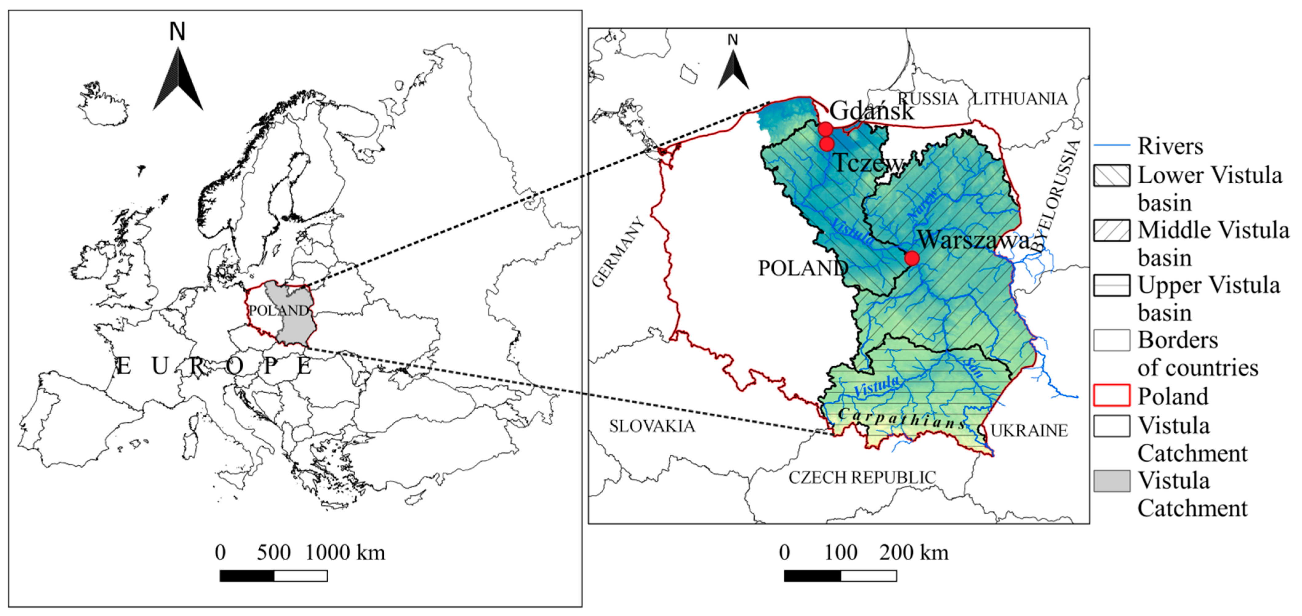
The Vistula River (Figure 1) is the longest and largest river in Poland, 1047 km in length. The drainage basin area is 193,960 km2, of which 87% (169,000 km2) lies within Poland. The remaining part of the basin is located in Belarus, Ukraine, and Slovakia. The Polish part of the Vistula basin covers 54% of the total land area in Poland. It has important social and economic significance. The basin is inhabited by more than half of Poland’s population. The course of the river from its sources to mouth is shown in Figure 1. Its average altitude is 270 m above sea level. Over three quarters of the river basin ranges from 100 to 300 m in altitude. The climate of the Vistula River basin is mainly continental, with variations between the mountainous southern part of the Upper Vistula and a wet, temperate climate at its lower northern part. Following the Köppen–Geiger classification as adapted by Peel et al. [19], the Polish climate is “cold,” with no dry season and with a warm summer (Dfb). In the Vistula basin, climate type Dfb prevails. In the south, there is also type Dfc (cold, no dry season, cold summer) and in the highest mountain parts type ET (polar, tundra).
The river in its middle and lower reaches creates numerous meanders and oxbow lakes. The Vistula is regulated from Tczew to Gdańsk. In its middle course there is a very valuable natural area occupied by forests, which are the habitat of many animal species.
In terms of land use structure, the largest area is arable land, occupying approximately 66% of the area, i.e., 120,000 km2. Forests and semi-natural ecosystems constitute 53,127 km2, or approximately 29% of the area. Urbanized areas cover about 6000 km2 (approximately 3% of the area), whereas water bodies in total cover 2833.2 km2, which is approximately 1.5% of the basin area.
As for hydrography, we distinguished three sections of the Vistula River and its basin: the Upper, Middle, and Lower (Figure 1).
The term Upper Vistula River applies to the 399 km-long section, from the source to the mouth of a right-bank tributary. The San and its Polish catchment area covers 46,000 km2. The 256 km-long Middle Vistula River begins from the mouth of the San and ends with the mouth of the Narew. Its Polish catchment area covers 89,000 km2. Some of the basin area lies in Belarus and Ukraine. The Lower Vistula River begins from the mouth of the Narew and ends with the Vistula’s mouth at the sea. It is 391 km long. The catchment area of the Lower Vistula covers 34,000 km2.
2.1. Spatial Diversity and Variability of Precipitation in the Vistula Basin
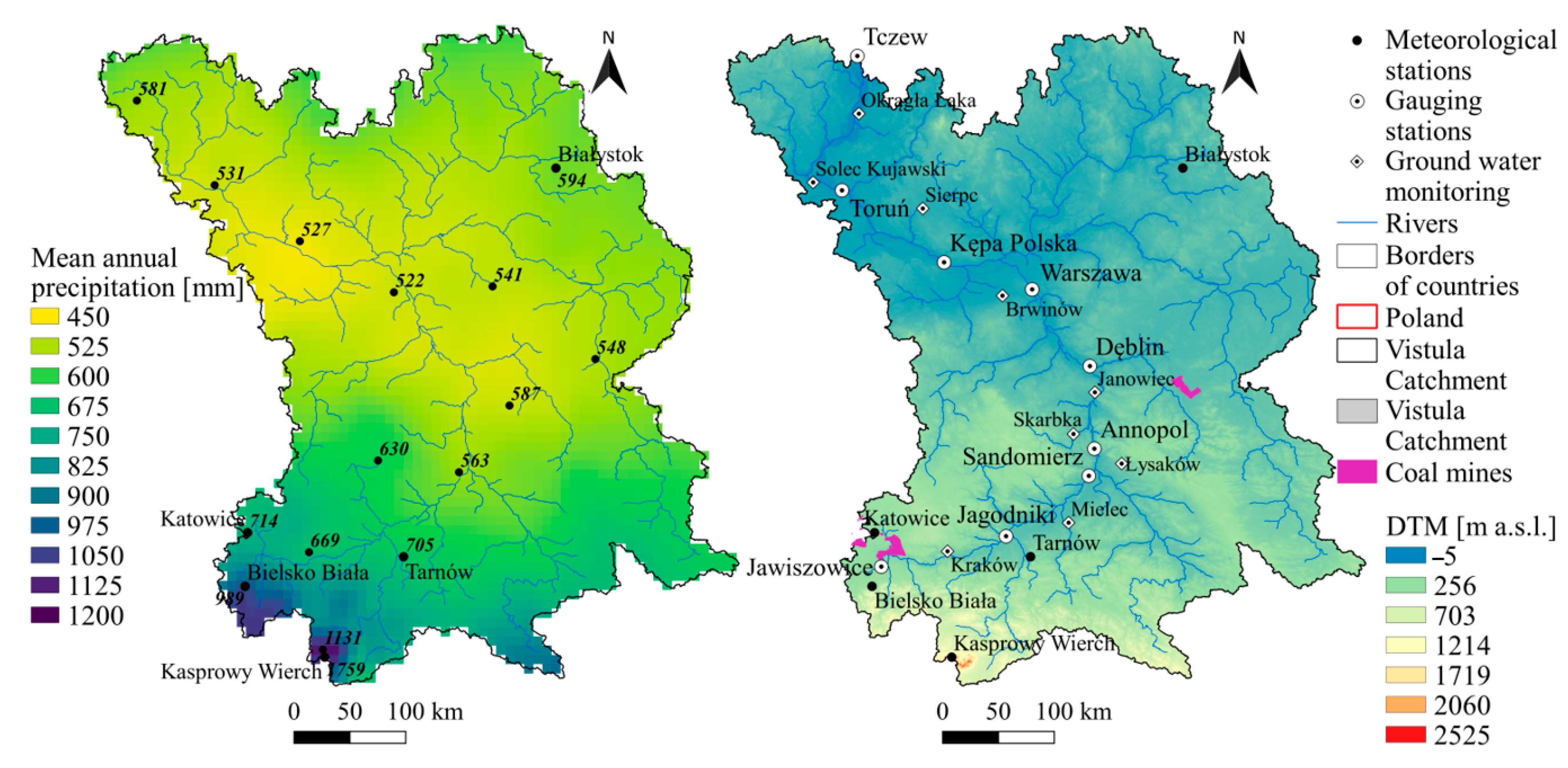
In the area of the Vistula basin, on average annual rainfall varies between 500–700 mm (with extreme annual precipitation at Kasprowy Wierch mountain station). Precipitation below 500 mm occurs only over a relatively small area of the river basin. It is the central area of the western part of the basin, where annual sums slightly exceed 500 mm. Increased sums in the range of 600–700 mm and more are noted in the uplands of the basin area. Within the Carpathian Mountains, there is a clear decrease in the annual rainfall from west to east, where they are only 850–900 mm. Rainfall in the range of 1000 to 1300 mm is recorded in the Bieszczady Mountains [21]. Information on some of the longest periods of precipitation from the basin are given in Table 1. The locations of the stations are given in Figure 2. The common observation period for meteorological stations covering the greater part of the basin area is usually shorter than 68 years, with records available for the flows. To ensure the best possible spatial coverage we decided to use data from the 1961–2017 period to derive precipitation-based indices (Section 4.4). The E-OBS 20.0e [22] provided spatially gridded precipitation records from the years 1951–2019; however, in this study we used data from meteorological stations because they are more accurate than gridded. The E-OBS data were applied to show the spatial distribution of precipitation presented in Figure 2 (left panel).
2.2. Surface Waters
Monitoring of surface waters in the Vistula basin is carried out in accordance with the State Environmental Monitoring (SEM) network and consists of 1617 measurement stations.
The list of sub-basins of the Vistula River corresponding to gauging stations located along the river is presented in Table 2. The characteristic features of the sub-basins are given, including the sub-basin area, a degree of human intervention (natural or altered), and the existence of water structures such as reservoirs, weirs, dams, and water transfer. In the last column the changes to gauging station locations are noted. The locations of gauging stations are given in Figure 2.
2.3. Groundwater Monitoring
Monitoring of underground water basins in Poland is carried out in accordance with the regulation on the form and method of monitoring groundwater bodies. In the area of the Vistula basin, the groundwater monitoring network, in accordance with SEM, consists of 710 points.
In the area of the basin, the highest degree of documented available resources was achieved in the middle and lower Vistula water regions, and the lowest in the Upper Vistula water region. In 2001 the concept of prospective resources was adopted and then estimated for the entire country [24]. The available and prospective groundwater resources in the basin are presented in Table 3. The locations of nine selected observation sites from the basin are shown in Figure 2. The sites were selected based on a number of criteria, the most important being the longest record without gaps longer than a month.
2.4. Human Interventions
The Vistula is under pressure from human activity like many other rivers in the world. It results from the population density of the river basin, agricultural purposes, forest and livestock management, and the provision of water for industry. The development of a hydro-technical infrastructure in the form of reservoirs and barrages, and the regulation of river beds, changes the conditions and distribution of flow over time. The impact of mine water discharges is especially significant in the upper part of the basin.
With regard to human activity data, the main problems arise from the fact that national databases identifying all types of pressures are often not spatially referenced. Most of the necessary data are collected there, but access to them is difficult or they do not cover all the period required. Moreover, the data are commonly stored in an administrative division framework that was modified four times in the last 70 years. Databases are scattered (not homogeneous) and often incomplete, even contradictory in different sources. For these reasons they could not be used in this study. An alternative approach is to use covariate [26,27] social, economic data (such as density of population and water use data, industry water use, agriculture yield, livestock, local gross domestic product, etc.).
The human activity pressures on water resources and the hydrological regime, especially accentuated in low flow periods, can be illustrated by the general structure of water use in Poland.
Over the last 20 years, a general decrease in total water consumption was observed, from about 11 km3 in 1998 to ca. 9.4 km3 in 2018. The total water use by industry also decreased from 8.1 km3 (73.7% of total consumption) to 6.8 km3 (61.8%). The consumption of tap water in households, hospitals, and shopping centers decreased from 1.9 km3 (17.2% of total consumption) to 1.7 km3 (15.1%) [28]. Throughout the study years, water consumption in households varied in cities and in the countryside. Consumption decreased in cities, regardless of their size, whereas in rural areas an increase was observed. The consumption per capita in cities remained higher by about 30% than in rural areas. The modernization of industrial plants by switching to closed water circuits, a significant increase in the price of water, the introduction of individual water meters, as well as the more and more commonly used water-saving devices for home furnishings have had a significant impact on this [28].
Water consumption for agriculture and forestry (including water used for irrigation of agricultural areas) remained on a rather stable level of about 1 km3, which corresponds to approximately 9–10% of total use [28]. The need to irrigation of plants results mainly from weather conditions. The immediate reasons for the application of this treatment on about 18% of the world’s area intended for cultivation is the constant or seasonal lack of precipitation. In Poland’s climatic conditions, irrigation is essentially interventional. Its main goal is to supplement the periodic rainfall deficits in the frequent but irregular dry periods, also known as agricultural drought periods [29]. It should be noted that the amelioration of agricultural areas in Poland was carried out in wet period, when the main problem was to drain the excess of water. Over the years the amelioration system has slowly lost its efficiency, caused by a lack of proper conservation and natural processes of silting and overgrowth of vegetation. Nowadays the system is being adapted to irrigation and together with modern irrigation technologies they can cope with shortages of rainfall using available surface or groundwater resources. To ensure access to irrigation water, a small retention program is implemented at the same time [30].
Due to topography, Poland is not a country with favorable conditions for the construction of storage reservoirs. There are currently 61 reservoirs with an area larger than 10 ha in the Vistula basin. Their total capacity is approx. 2860 million m3, which is only 8.6% of the mean total annual runoff to the Baltic Sea.
One of the most important human pressures on water regime and water quality in surface waters of the Vistula River is the coal mining industry seriously damaging the environment in the mining area. Coal mining activities impose harmful, usually irreversible impacts on the terrestrial and aquatic environments not only in situ but also on long reaches downstream from the injection of mining waters.
In the 1967–2013 period on average 7.94 m3/s of mine waters coming from the drainage of hard coal mines in the Upper Silesia Coal Basin (USCB) were discharged to the Vistula River. The maximum discharge was reached in the period of the largest extraction, i.e., the years 1979–1989, and especially 1985–1988 [31].
The second coal mine area is located in the Middle and Lower Vistula basins, in the Bug and the Wieprz basin tributaries (see Figure 2). The coal deposit covers an area of 4000 km2, is 180 km long, and approx. 22 km wide [32]. Currently, there is only one active mine, “Bogdanka,” which discharges pre-treated mine water at an average rate of 0.17 m3/s to the Swinka River—the tributary of the Wieprz [33].
The plans to restructure the mining industry in Poland launched in 1989 with the goal of reducing the proportion of coal energy in the domestic energy budget and focusing on searching for methods of diversification of independent energy sources resulted in successive limitation of coal extraction mainly by closing mines. In the last years the total hard coal extraction reached the levels from the early 1950s. However, even after the mine ceased operation, in most parts of the USCB mine water has had to be drained due to the risk of methane accumulation and explosion. Therefore, despite the corrective actions, it is necessary to wait for the specific effects of the actions taken. Then the problem can be posed regarding how the cutoff of mining water discharge will affect low flows, keeping in mind their share in the recipient flow.
3. Methods
Wu et al. [34] showed that human-induced changes are more visible during the high-flow seasons whereas climate change influence on flow regime is more visible during the low-flow seasons. Those results indicate that catchments’ response to changes in external forcing depends on catchment wetness conditions at the start of the event. The validity of this hypothesis can be assessed by the division of the annual period into summer and winter periods and statistical analysis of a number of drought indices. The analysis presented here includes an application of statistical analysis of mass curves of mean annual (MQ) and mean seasonal flow and annual and seasonal minimum flow in the reduced variable coordinates along the course of the Vistula River, baseflow, and standardized drought indices. Rank correlation analysis was applied to study the relationship between standardized drought indices and their dynamics.
3.1. Mass Curve Analysis
A convenient tool for detecting the wet and dry periods and their length is well embedded in hydrology, notably, a mass curve technique, especially when presented in a reduced variable system. The mass curve is a plot of the cumulative values of a variable as a function of time (e.g., [35]). It is applied especially to mass curves of rainfall or runoff to show deviancies of various meteorological or hydrological elements from uniform conditions for the analyzed period (straight line from the zero value at the beginning of the observation period to the total value at the end). The plot in reduced variable coordinates shows the differences between observed cumulative values and the cumulative mean value for the entire period. An increasing limb of the plot indicates wet periods, and a decreasing part, dry periods.
3.2. Baseflow Filtering Method
Baseflow is a river discharge fraction that is strongly correlated with groundwater [36]. Though such processes continue to be problematic for determining and visualizing, the estimation of groundwater inputs to river flow is highly significant for estimating river flow [37]. A baseflow program [38], an automated baseflow method, is used to separate baseflow from streamflow. Based on the assigned baseflow estimates used, automatic filtering is applied three times (forward, backward, and forward) via streamflow data and provides baseflow as a percentage of the total flow using the following equation to determine the direct runoff and baseflow [38]:
where is the baseflow in time t, is the filtered surface runoff, is total streamflow in time t, and β is a filter parameter, which is equal to 0.925.
3.3. Standardized Drought Indices
According to Mckee et al. [39], the long-term precipitation data for the Standardized Precipitation Index (SPI) estimation at a target timescale would be assigned to a probability distribution function, which is again converted into a normal distribution function. Following the procedure described by Mckee et al. [39], at each running month, a distribution function is fitted to precipitation values accumulated over the selected number of past months from the long-term monthly precipitation data set (so-called reference data). This distribution function is then transformed into a Gaussian distribution in order to allow for the comparison of the drought index between catchments. The fitting of a theoretical distribution can be replaced by an application of an empirical distribution function [40]. Then for each month, the inverse of a Gaussian distribution function is found as the appropriate SPI value based on the empirical probability derived from precipitation events over the period of aggregation [41]. The choice of that accumulation or scaling period depends on the detail needed to study the drought event and the purpose. Usually 3-month, 6-month, 12-month, and 24-month accumulation periods are applied. A three-month accumulation period is suited to study soil moisture conditions, whereas the longer time periods would better describe long-term drought events. Therefore, the SPI depicts the deviation of an event from the long-term mean. A similar approach is used for the derivation of the other standardized indices. Both parametric and non-parametric methods can be applied depending on the time-series characteristics [40]. As shown by Blain et al. [42], gamma distribution commonly fits the precipitation data. The two parameters of the distribution can be estimated using the maximum likelihood method and then converted into the cumulative probability distribution.
Modarres [43] introduced the Standardized Streamflow Index (SSI) for a reference period of each hydrological year based on the cumulative runoff volume using the monthly runoff volume series. In this study, we used the log-normal distribution with two parameters, and then the distribution was transformed into a normal distribution similar to the SPI discussed above.
The Standardized Precipitation–Evapotranspiration Index (SPEI) was developed by Vicente-Serrano et al. [44] based on the climatic water balance using precipitation and potential evapotranspiration data to incorporate the effects of temperature changes on drought assessment. The climatic water balance , which provides a simple measure of the water surplus or deficit for the analyzed month, is computed as follows:
where and are the depth of precipitation and potential evapotranspiration, respectively, for each month i.
The simulated monthly climate water balance is then accumulated to the desired time scales using the same procedure as for the SPI, except that the distribution of the three-parameter, log-logistic distribution is used to determine the SPEI instead of the two-parameter gamma distribution [44]. The temperature-based potential evapotranspiration developed by Hargreaves and Samani [45] was applied in this study.
Baseflow data filtered by the automatic baseflow separation method are used in the SSI discussed above to estimate the standardized baseflow index (SBFI) to determine groundwater dryness.
In addition, the Standardized Groundwater level Index (SGI) is derived using a similar approach as for the SPI index. Bloomfield and Marchant [46] applied an approach consisting of a nonparametric normal score transform of monthly groundwater levels, as each of the observation sets used required a different probability distribution. The same method was applied in Liu et al. [47] in the analysis of groundwater level observations in Jiangsu Province, China. In that approach, a probability value is assigned to the monthly groundwater levels based on their rank in that month for all the available years. In the next step the inverse normal distribution is applied to those probability values to obtain the SGI values. This transform gives an SGI distribution that will always pass the Kendal–Stuart normality test [48].
3.4. Drought Characteristics
To quantify the impact of a drought and assess various drought characteristics such as duration, intensity, and severity, a drought index is the primary parameter. Among the drought indices (DI) applied in this study, there were two meteorological indicators (SPI and SPEI), two hydrological indicators (SSI and SBFI), and one groundwater indicator (SGI). As shown in Table 4, drought events are categorized based on the drought index value, as found in Mckee et al. [39].
A threshold of −1 was used in this analysis to define drought. Meteorological and hydrological drought in this sense began when the DI values were equal and lower than −1 and ended when the DI values were positive. The drought duration DD is a period during which the values of the indices under consideration (DI) remain below the defined threshold value; the absolute value of the total value of DI within DD is defined as the severity of a drought (S); the ratio of the severity of a drought to its duration is the intensity of a drought (I) [39].
4. Numerical Results
4.1. Statistical Analysis of Annual and Seasonal Mean Flow Patterns along the Course of the Vistula River
There are two major driving forces affecting the water cycle and consequently the riverine hydrological regimes: climate (variability and change) and human activity. The long-term data are indispensable for quantifying their effects on hydrological regime. The hydrological data from nine gauging stations situated along the course of the Vistula for the 1951–2018 period were used in this study (Figure 2, Table 2), as well as several selected precipitation stations distributed within the Vistula basin with the 1951–2019 observation period (Table 1). The data were checked for absent observations and homogeneity. Short gaps were filled by interpolation. The selection of gauging stations ensured the homogeneity of the observations.
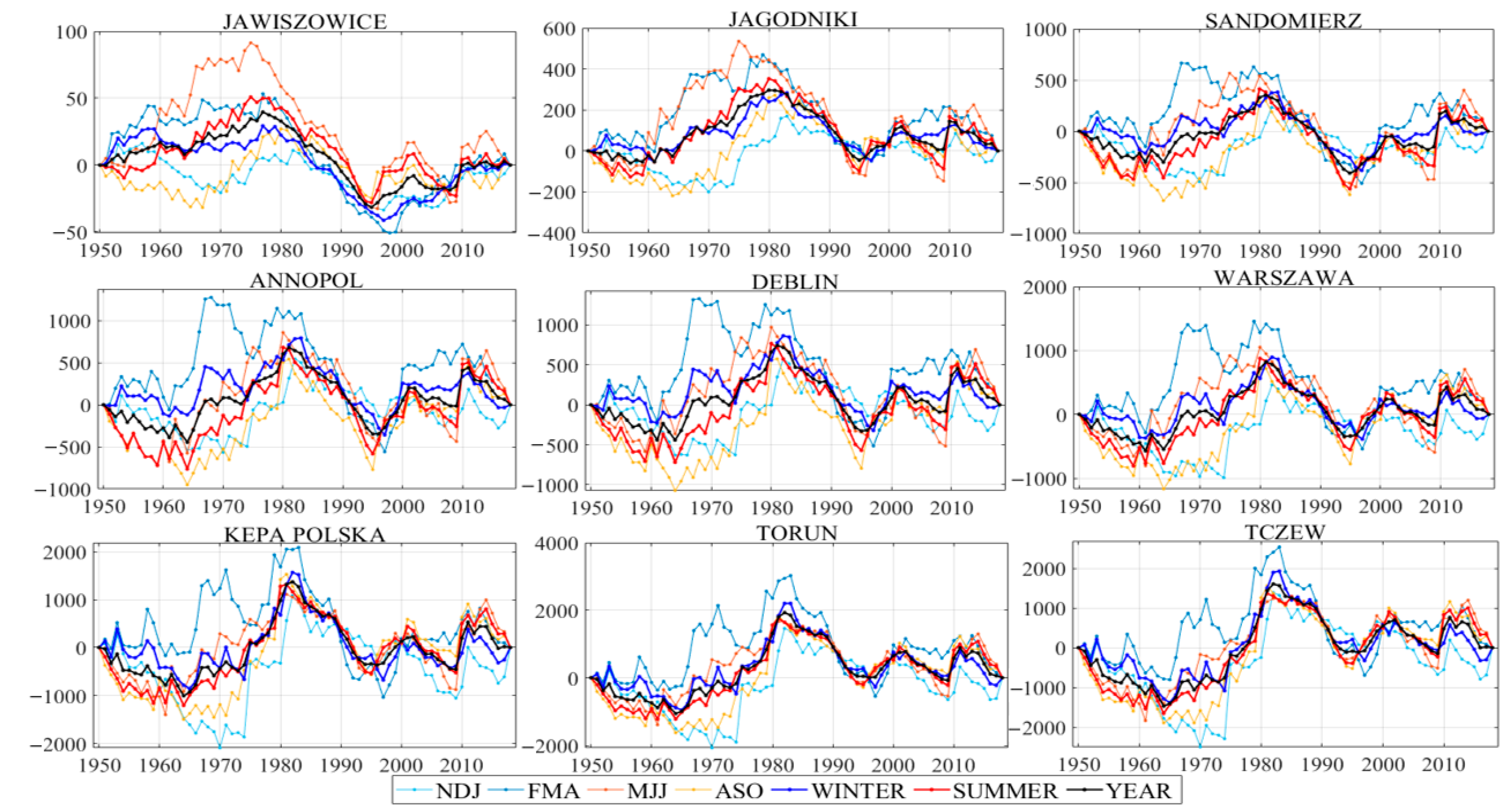
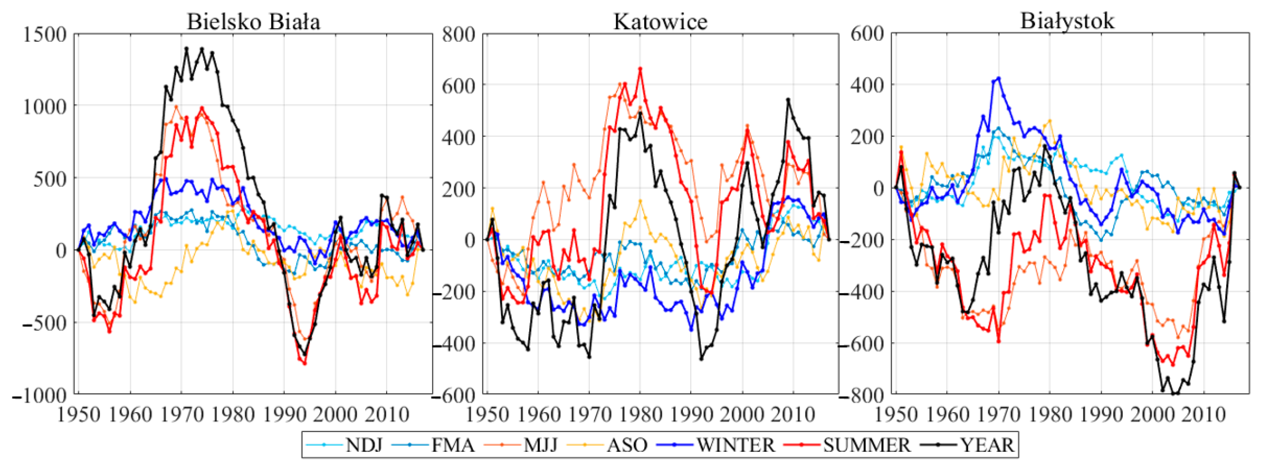
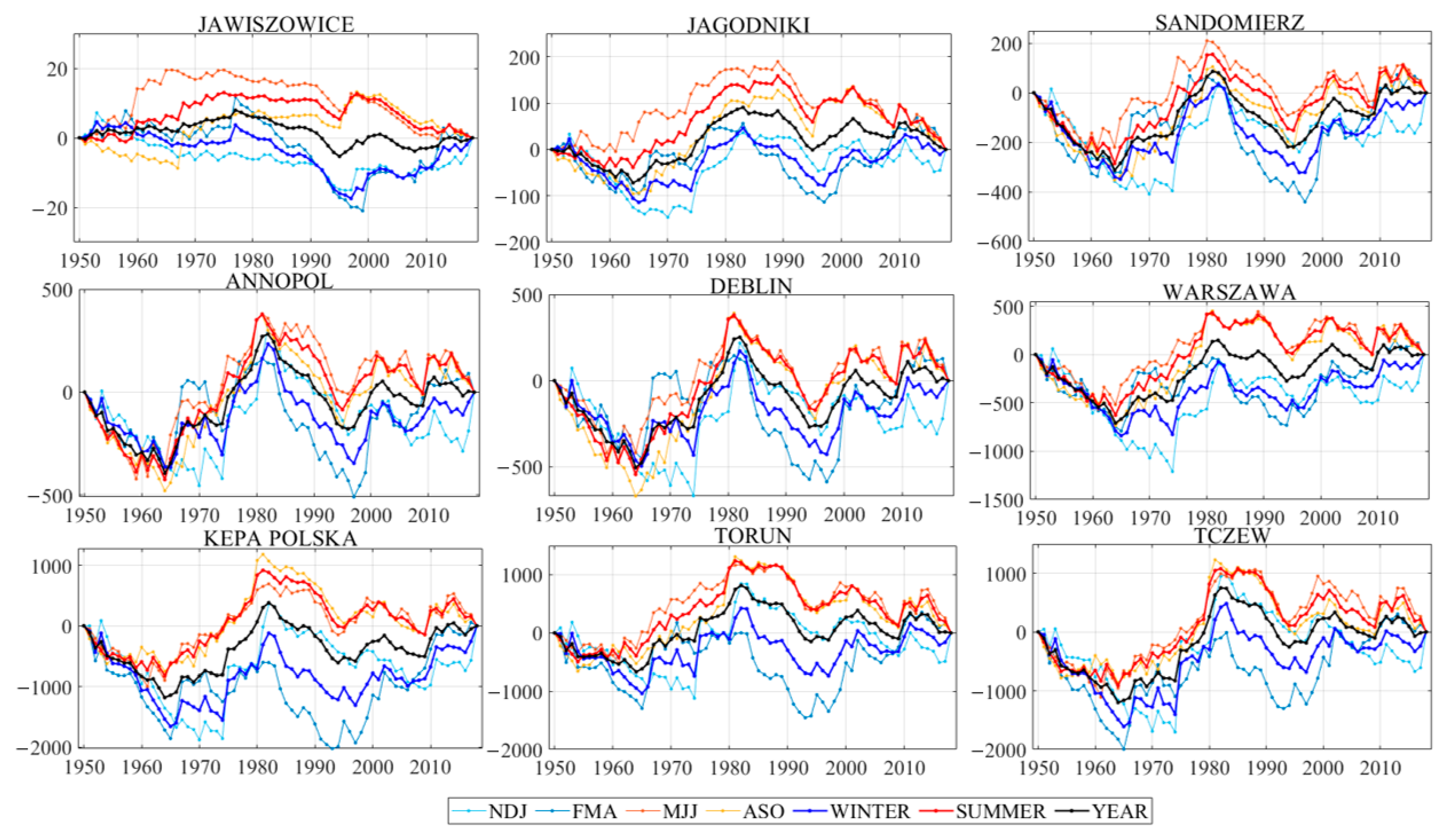
In Figure 3 mass curves of mean annual flow (MQ) in the reduced variable coordinates along the course of the Vistula River are presented for the selected gauging stations. Apart from annual (year) and warm half of the year and cold half of the year curves, also shown are the seasonal curves for spring, summer, autumn, and winter. In the analyzed multiannual period, the pattern of wet and dry spells remained almost stable along the river from Jawiszowice to the closing station at Tczew. The first dry spell lasted from 1951 to approximately to 1964; the succeeding wet period lasted until the early 1980s. Then two less pronounced wet and dry periods were observed. Upstream stations Jawiszowice, Jagodniki, and Sandomierz revealed slightly different patterns. This was an effect of the catchment size and anthropogenic pressures in this area, i.e., Goczałkowice reservoir with water intakes for the Katowice conurbation and other cities of the Upper Silesia and especially in the Upper Silesian Industry District (USID) with water transfers between the Vistula and Odra basins. Other pressures on flows of the Upper Vistula River were mining waters injected into the Vistula River and its tributaries from mines in the USID. Even after the mine ceased operation, mine water had to be drained due to the risk of methane accumulation and explosion.
It is worth noting that even important tributaries such as the San or the Narew did not change pattern significantly in the main stream of the Vistula. Therefore, it can be concluded that the impact of human activity on the mean discharge of the Upper, Middle, and Lower Vistula River is irrelevant in the face of climate drivers.
The winter and summer mass curves differed from each other only for Jawiszowice along the whole time period under study and showed some differences in the 1950s and the 1960s for the other stations. However, more variability can be seen in the quaternary seasonal patterns, in particular in the period ending in the mid-1980s.
It is useful to compare the flow pattern along the Vistula River course with precipitation. For the purpose of this study only three precipitation stations were selected for comparison. The choice of the stations was dictated by their location, the length of records, and climatic diversity. It was not possible to estimate the precipitation on the sub-basin areas of the Vistula basin due to the lack of data for the entire analyzed period. Therefore, the comparison is only illustrative.
The patterns of wet and dry periods in annual and seasonal precipitation totals presented in Figure 4 are generally similar to the patterns presented in Figure 3; however, this similarity is not close. In particular, Bialystok had a slightly different pattern of dry and wet periods, especially in the winter season. This station is located in northeastern Poland and is under the influence of a continental climate.
The main flow characteristics for the stations located along the course of the Vistula River are presented in Table 5.
The highest of the high flows in the period (HHQ) and the lowest of the low flows (LLQ) present the range of flow values measured at each gauging station. Looking at the seasonal variability, the summer season provided the highest of the high flows at all stations. On the other hand, the lowest of the low flows (LLQ) was mostly observed in the winter time, with the exception of Jagodniki and Torun. The mean highest flow (MHQ), the mean flow (MMQ), and the mean lowest flow (MLQ) tell us about water volumes transferred in the system down the river in each season and annually.
4.2. Statistical Analysis of Flow Minima along the Course of the Vistula River
Figure 5 presents a mass curve analysis of minimum flow for a year and the winter (cold half of the year) and summer (warm half of the year) seasons, and also for the three-month periods. The variability of drying and wetting periods was larger in comparison with the mean flow patterns, which is not surprising. We can see the largest differences in the stations located downstream (Kepa Polska, Torun, and Tczew) which might be related to the influence of a large tributary, Narew, at low flows.
Analysis of the dates of low flow occurrence (not shown) indicated that at the furthest upstream station (Jawiszowice) there was no specific low flow season. The lowest seasonal low flow occurred at any time of the year. However, at the stations located downstream (Jagodniki) the lowest flows practically did not occur in the March–June span. This information can be helpful in the analysis of low flow periods.
The results of the Mann test for trends in the winter and summer minimum flows and the Pettitt test for change-point detection [49] are presented in Table 6. There was a significant positive trend detected for Sandomierz and Warsaw for the winter season. For Jagodniki there was a positive significant change detected in two years, 1966 and 1989. As this gauging station is situated in the area affected by the mining industry, that trend could be associated with human activity. Warszawa showed a significant positive trend and a significant positive shift in winter 1974. Of the stations situated in the lower Vistula, Kepa Polska showed a significant positive shift in winter 1966. Torun showed a significant negative trend for summer and a significant negative shift in trend in summer 1989.
Table 7 presents the results of the Mann test for the trend of the annual minimum flows and the Pettitt test for change-point detection. A significant positive trend is shown for three gauging stations, Sandomierz, Deblin, and Warszawa. A significant positive shift in trend values in the same year, 1964, is shown for four gauging stations, Jagodniki, Sandomierz, Annopol, and Deblin, and also for Warsaw in 1974 and Kepa Polska in 1973. Only the Warsaw results are consistent with seasonal results for winter low flow at the Warszawa gauging station.
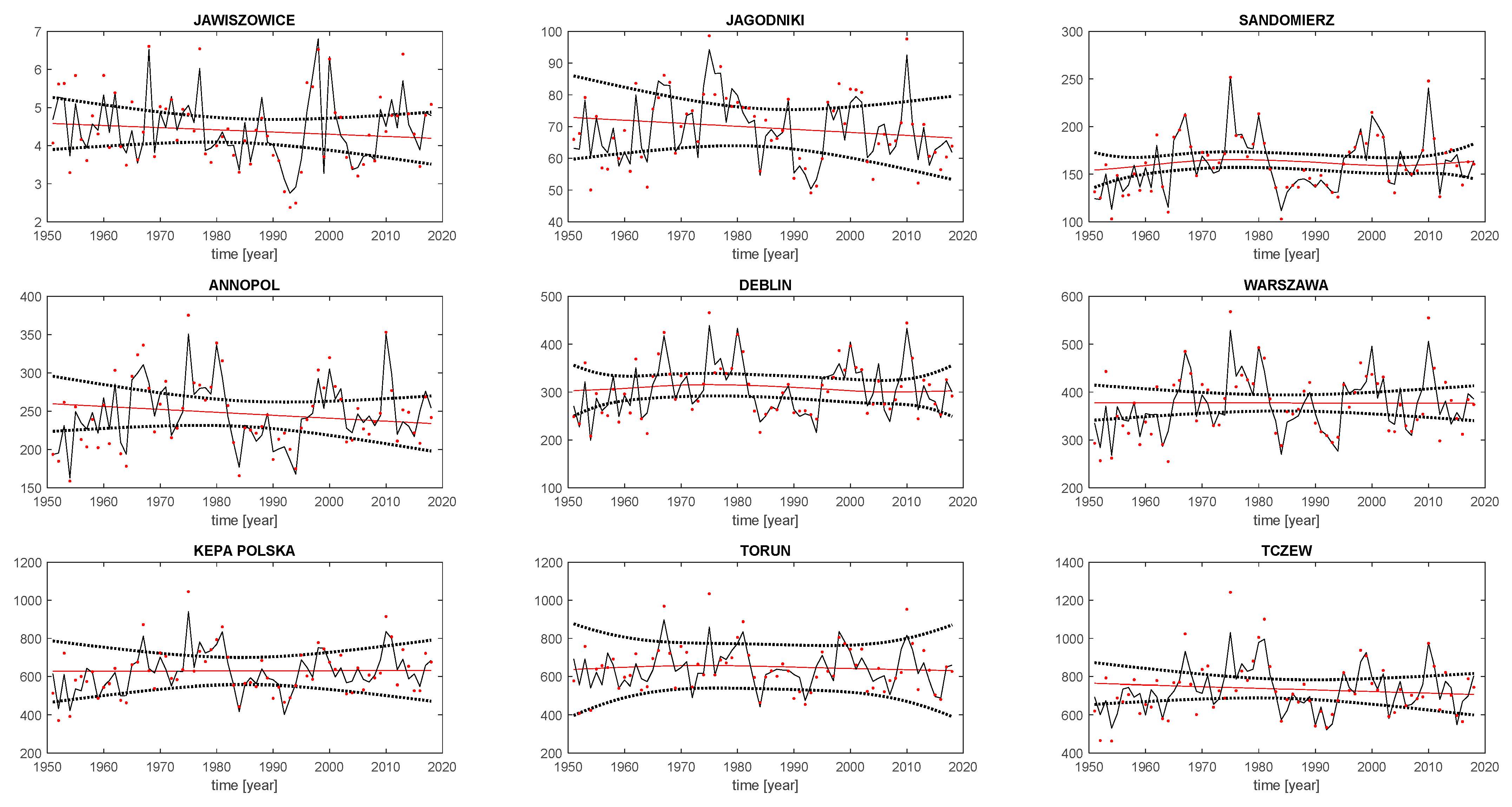
In order to further illustrate trend analysis, we performed a dynamic harmonic regression analysis (DHR) of minimum annual flows. This approach was successfully applied to analyze trends in flows by Meresa et al. [50]. DHR belongs to parametric methods of trend estimation [51]. The method assumes that time series can be modeled by the so-called “unobserved component” model, being a sum of a non-stationary long-term trend and cyclic/seasonal components. The temporal patterns in data are modeled within a stochastic state space formulation. The time-varying parameters of the model are obtained using an optimal estimation method based on the Kalman filter. The DHR algorithm is available in the CAPTAIN Toolbox for Matlab™ [52]. As the method is statistically based, trend estimates have associated measures of confidence (standard error bounds). A normality test is applied to assess the statistical significance of a trend [53]. This test takes into account the uncertainty of trend estimates and therefore is more robust than the other commonly used tests.
According to the normality test with uncertainty of trend estimates taken into account, none of the trends presented in Figure 6 were statistically significant. This shows that in the presence of uncertainties eye inspection may fail.
4.3. Transformation of Hydrological Drought along the Vistula River
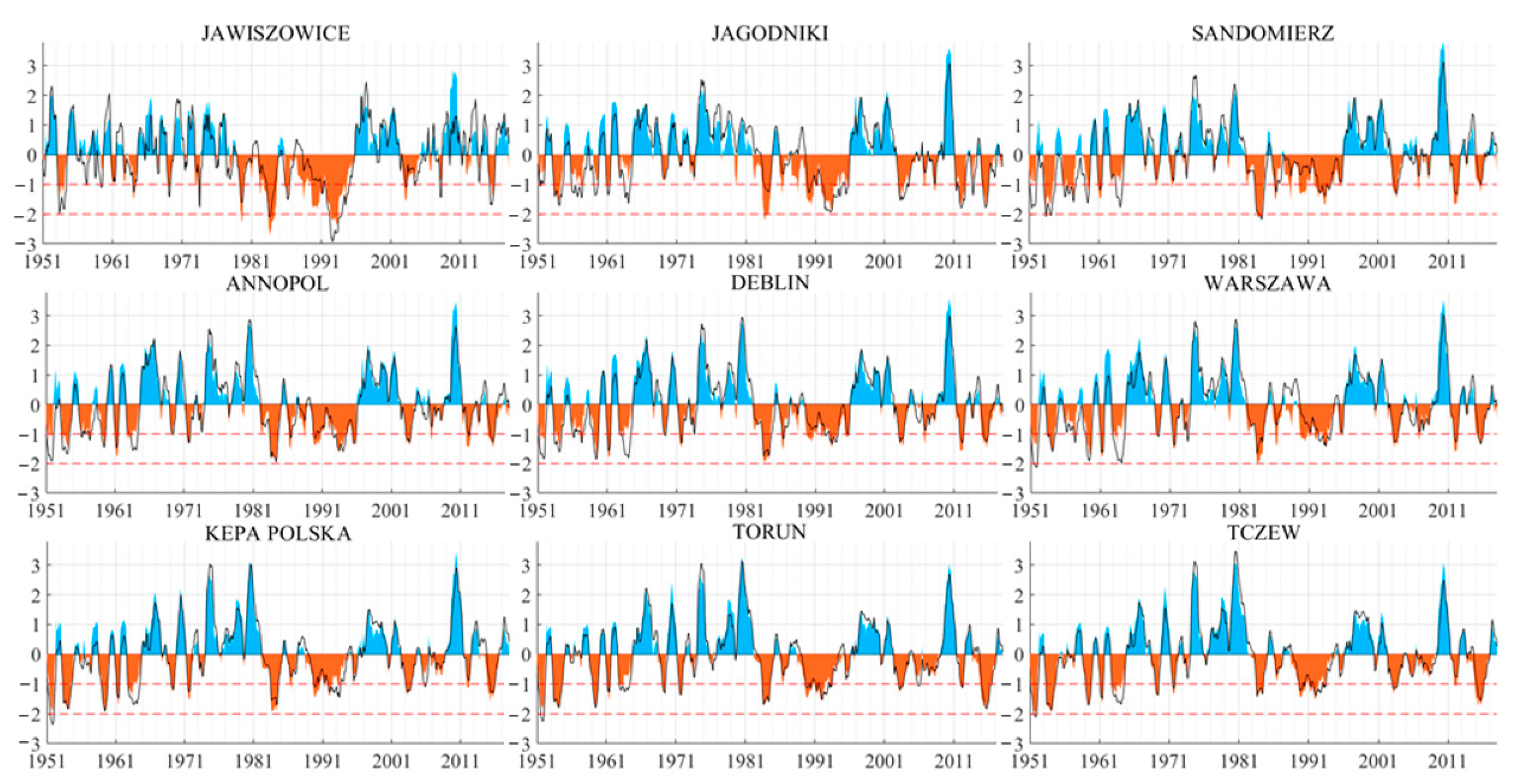
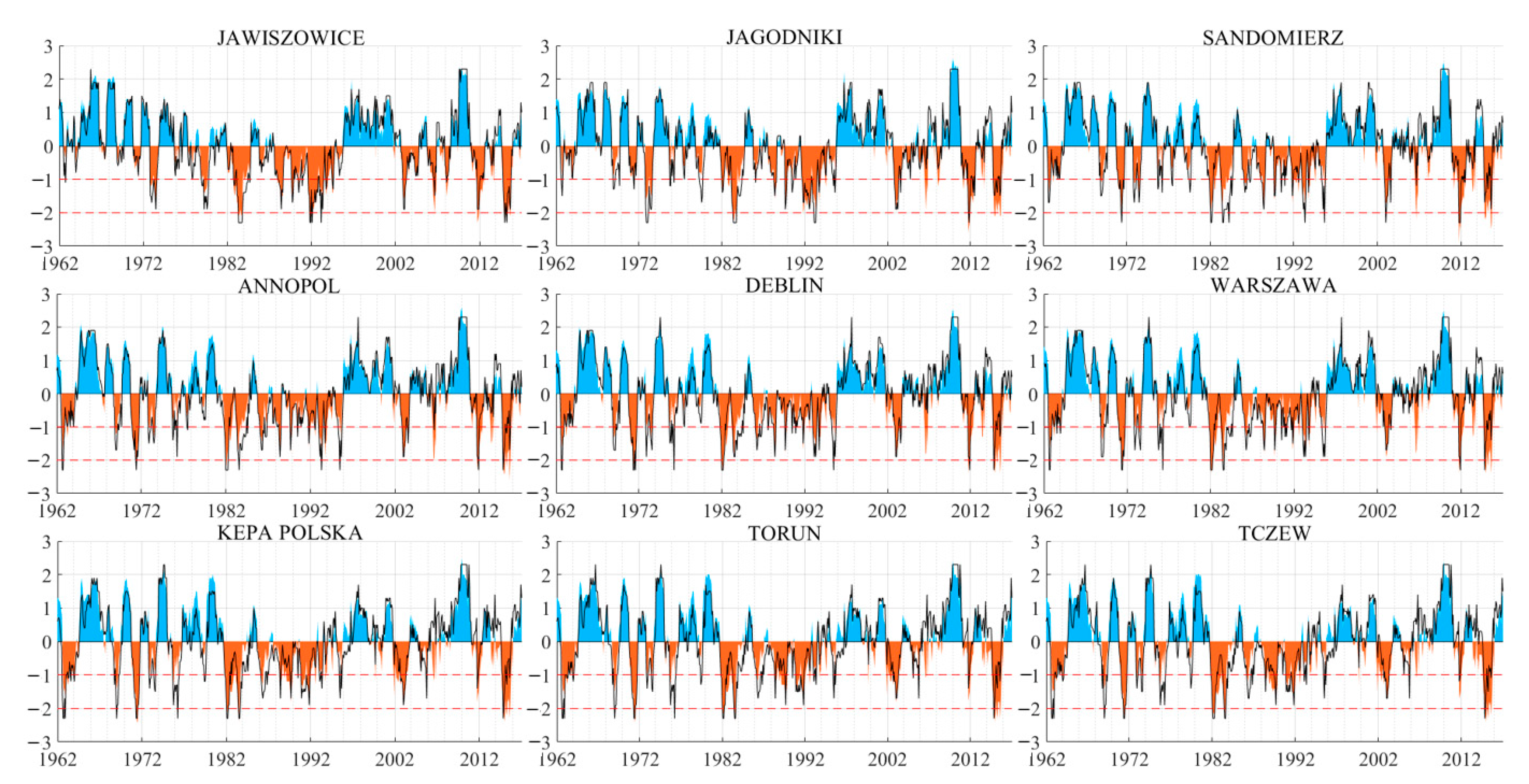
The flow values measured at nine gauging stations were used to derive a standardized streamflow index in order to quantitatively assess the appearance and transformation of drought conditions along the river. As described in Section 3.3 there are different accumulation periods possible. Their choice depends on the character of the drought events of interest. The period usually varies between three and 48 months. The longer periods better describe more persistent droughts than the shorter periods. However, an increase in period leads to a decrease in index clarity in finding short-term variations in flow. Here we decided to choose the 12-month aggregation period for all indices studied to get sufficient accuracy without too much variability shown. Flow measurements were used to derive baseflow using the filtering approach [38]. In order to illustrate how the drought characteristics transformed along the river with the flow, both the SSI12 and Standardized Baseflow Index SBFI12 were derived for the selected gauging stations for the entire 1 November, 1950–31 October, 2018 observation period. A comparison of SBFI and SSI at a 12-month accumulation scale is presented in Figure 7.
As shown in Figure 3, Figure 5 and Figure 7, the hydrological drought patterns corresponded with the drying and wetting spells presented by the mass curve plots and standardized hydrological drought indices. From Annopol downriver, a long-term dry spell was seen, then long wet and dry spells, followed by shorter dry (1983–1996 and 2003–2009) and wet (1997–2002) periods. The year 2010 was very wet, but in the whole period from 2002 onwards, dry spells prevailed.
The differences between SSI and SBFI reflect the differences between streamflow and baseflow distribution patterns. They are visible at extreme values and in the start and end times of the drought episodes.
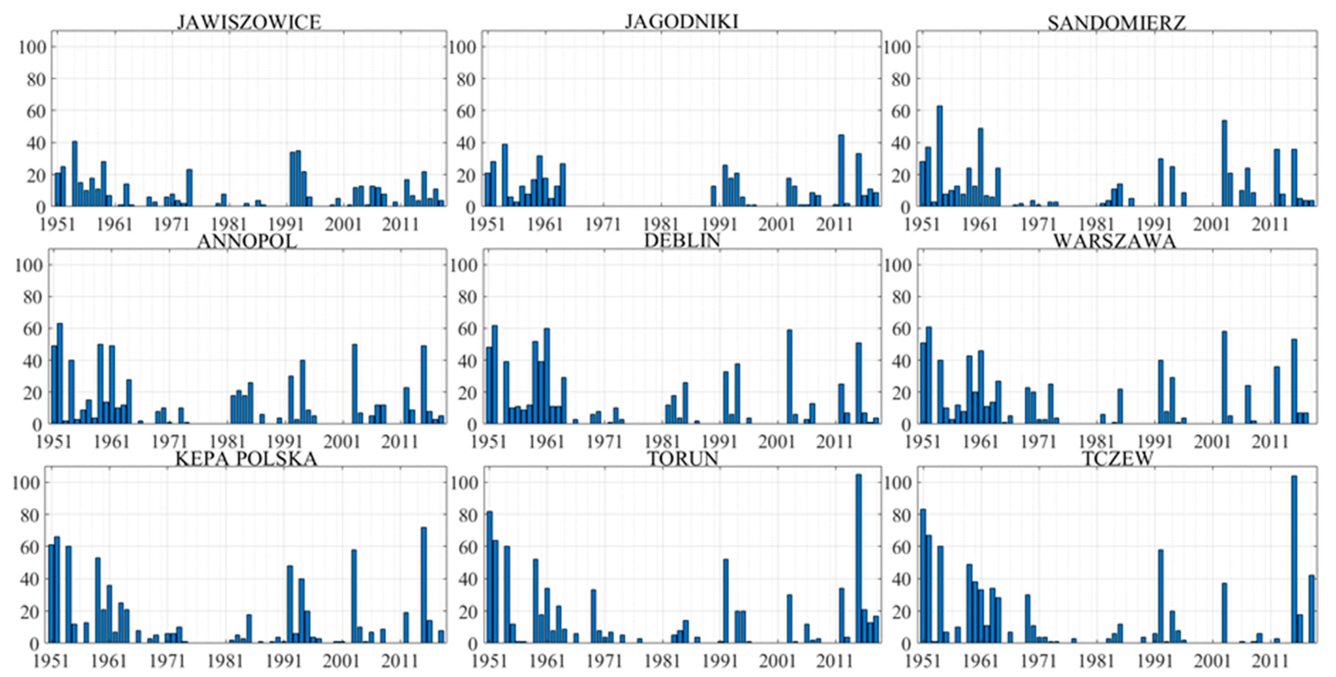
A comparison of the longest period (days) with flow below the 0.05 quantile for nine gauging stations along the Vistula is shown in Figure 8. It illustrates the propagation of drought along the river. As human interventions are present only in the upper part of the Vistula and only the first three stations can be affected, the lower part starting from Annopol down to Warszawa should follow natural climatic forcing.
Downstream of Warszawa there is a large tributary (Narew) that can change the low flow conditions in Kepa Polska. The last two gauging stations, Torun and Tczew, showed increasing drought severity. In both cases the largest number of days with very low flow exceeded 100 in 2015. This illustrates that the river becomes drier along that particular reach.
4.4. Transformation of Meteorological Drought into Hydrological Drought along the Vistula River
A number of drought indices, including SPI, SPEI, SSI, and SBFI, were derived for 56 years (1961–2017) using hydro-meteorological data from the Vistula basin. Daily precipitation data collected from 48 meteorological stations within and surrounding the basin were used for the interpolation of precipitation fields for the sub-basins and for the derivation of the SPI and SPEI indices (the meteorological stations were selected in such a way as to ensure the best possible spatial coverage, with a sufficiently long common observation period). The quality of the data was checked, and missing data were filled by the normal ratio method using neighboring stations. The weighted areal precipitation over the basin was calculated using the Thiessen polygon method over nine sub-basins along the main river course considered in the study. Finally, the daily data were aggregated to monthly precipitation data, which were used as input for a meteorological drought assessment. Monthly time series of precipitation, temperature, streamflow, and groundwater discharge were used to determine meteorological-, surface water-, and baseflow-related drought.
As in the previous section a 12-month aggregation period was applied to derive the standardized indices. Figure 9 shows the estimated SPI12 and SPEI12 values for the Vistula River for the years 1961–2017. Both indices showed very similar temporal and spatial (with the river flow) variability. Considering the SPI12 reference period with a value below the threshold of −1, 22–33 drought events happened at different locations in the basin between the hydrological years of 1961 and 2017. The results show that historical drought durations of more than five months occurred in 1963, 1970, 1972, 1977, 1983, 1984, 1987, 1992, and 2004 at Tczew gauging station, whereas for the gauging stations near the headwaters, at Jawiszowice, drought events with a duration of more than five months happened mainly in 1974, 1980, 1985, 1989, 1993, 2003, 2012, and 2016. Although the severity of drought varied temporally and spatially, the most severe drought of the longest duration occurred from the 1980s to the beginning of the 1990s (from 1982 to 1993). Both indices show that the maximum drought was more pronounced in Tczew than in the upstream sub-catchments such as Jagodniki and Jawiszowice. The results show that the consideration of potential evapotranspiration changed the drought estimates only slightly when examined over a 12-month aggregation period.
Spatial and temporal variations of meteorological and hydrological drought using the same 12-month time scale, SPEI12 and SBFI12, are shown in Figure 10. Figure 10 also shows that the timing of peak drought and duration varied between meteorological drought and hydrological drought, showing a delay in propagation from meteorological drought to hydrological drought.
In Figure 11 the summary of a number of drought events, maximum duration, mean duration, and mean drought severity is presented for all the gauging stations and four different standardized drought indices (SPI12, SPEI12, SSI12, and SBFI12) for the 1961–2017 period. The number of events was higher for meteorological droughts and lower for streamflow-related droughts (SSI and SBFI), with a slightly smaller number of events at the last three sub-basins downstream. In contrast, for both surface flow and baseflow, mean drought severity and mean drought duration were higher and longer, respectively, at the upstream end and near the outlet of the watershed than in the middle of the watershed. The 1991–1993 drought was the most severe, with the longest durations of 35 and 39 months of historical droughts occurring for baseflow and streamflow, respectively. In general, drought intensity was higher for baseflow than for streamflow.
Comparing meteorological drought to hydrological drought shows that the number of drought events decreased whereas the mean severity and duration of drought increased in all sub-basins of the study area (Figure 11).
The Standardized Groundwater level Index (SGI) was computed for nine wells located near the sub-basin gauging stations. Unfortunately, the groundwater measurements were of much poorer quality than the flow measurements and the longest time series started in 1991. Weekly observations were homogenized and the missing data were filled by linear interpolation. We applied a non-parametric approach for the derivation of SGI12 [40] and we compared the results with a parametric approach using the gamma distribution to fit the 12-month data. The results of SGI12 for nine measurement sites corresponding to nine sub-catchments according to their location are presented in Figure 12. The results of SGI12 showed low water levels for the 2003 drought and some wells showed long-term drought conditions in the 2001–2015 period.
Interesting relationships are shown by comparing the results of the analyzed indicators. Figure 13 shows the results for all analyzed indicators for the 12-month accumulation. The reduction in the number of locations for which the results are presented was due to the common length of consistent observations needed to determine the analyzed DI. Each clearly marked drought period for the meteorological indices (SPEI, SPI) was accompanied by a similarly marked period for the hydrological indices (SSI, SBFI), with a time lag with respect to the meteorological index. Meteorological drought also translated into a reduction in groundwater levels, expressed here by the SGI indicator. Periods with negative values of SPI and SPEI were followed by a decrease in SGI values, not always leading to exceeding the zero threshold value. The translation of periods of meteorological to hydrogeological drought was not as unambiguous as in the case of hydrological drought. A greater temporal shift was observed in subsequent meteorological and hydrogeological droughts, not always preserving temporal relationships in the occurrence of subsequent periods. This was due to different properties of the permeable ground, location of zones feeding a given groundwater reservoir, and the time resilience depending on the size of the groundwater reservoir for which groundwater table levels were measured.
4.5. Correlation between Drought Indices
Spearman’s rank correlation coefficient [54] was derived for drought indices SPEI12 versus SSI and SBFI at different accumulation times (Figure 14). A non-parametric approach was used for the derivation of those indices to avoid an influence of distribution fit on the results. The best correlation between SPEI12 and SSI was obtained for three sub-basins, with discharge at gauging stations Annopol, Deblin, and Warszawa for the nine-month accumulation time, whereas Kepa Polska, Torun, and Tczew showed a smaller correlation between 0.58 and 0.7, but still with the peak for a nine-month accumulation. The most upstream sub-basins, delineated by the stations Jagodniki, Jawiszowice, and Sandomierz, had the best correlation for the 12-month accumulation time with a maximum correlation between 0.6 and 0.7.
The dependence of the correlation between SPEI12 and SBFI for different time accumulations is presented in Figure 15. We found similar clusters of sub-basins as for the SPEI–SSI relationship, i.e., the most upstream sub-basins, including Jawiszowice, Jagodniki, and Sandomierz; the second including Annopol, Deblin, and Warszawa; and the third including the lowest sub-basins, defined by the stations Kepa Polska, Torun, and Tczew. The second cluster had the highest correlation with SPEI at the nine-month accumulation time and the first cluster also had a maximum at nine months of accumulation, but the last cluster (Kepa Polska, Torun, and Tczew) had maximum correlation with SPEI12 at six months of accumulation.
5. Discussion
We see the study as being a template for the reconnaissance of drought conditions in any river basin. The novelty of the approach is a comparison of current hydrological practice (mass curves) with the utilization of drought indices. The approach complements the practical approach illustrating dry/wet periods with quantitative, index-based analysis.
Taking into account the mass curve patterns of mean flow presented in Figure 3, it can be argued that the changes in water balance in the Vistula River basin caused by warming and increased potential evaporation were small in the analyzed period and did not cause significant or relatively permanent changes in the annual or seasonal patterns of the river flow. In addition, the influence of other anthropogenic factors (e.g., regulation of rivers, water intake and discharge, urbanization), although visible locally on the scale of rather small catchments, has not yet translated into permanent, regional changes. A comparison of the mass curves obtained for the mean annual flow with the mass curves for the precipitation (Figure 3 and Figure 4) shows that climate factors are the main driving force of a clearly visible sequence of wet and dry spells.
An analysis of the lowest seasonal flows (Figure 5 and Table 5) provides useful information on their variability over time, although one should be aware that the expected causes of changes in these values, in addition to climate change and pressure from human activity, must include time shifts of low-flow phenomena (also dependent on these factors) when the lowest flow of the low-flow period occurs already in the next season. However, these are not frequent cases. In this study only the lowest seasonal and annual flows were examined. In Table 5 one can find the lowest (LLQ) and the mean lowest (MLQ) seasonal and annual flows observed at nine selected gauging stations along the course of the Vistula River. In the analyzed period, the values of LLQ and MLQ were rather balanced in both seasons, and the share of winter minima in the annual minima in the Upper, Middle, and Lower Vistula reaches varied from about 40% (at Kępa Polska) to about 50% (at Dęblin).
The analysis of trends and points of change of seasonal and annual LQ flows included the Mann test for the trend and the Pettitt test for the jump in mean value. The results are summarized in Table 6 (seasonal analysis) and Table 7 (annual minima analysis). It is worthy of note that the results of the change-point detection in a seasonal frame differed from those obtained in annual minima testing. The annual approach masked some seasonal trends and revealed others. The differences in change point of the annual LQ were more stable—the detected change point in the annual minima LQ was in the year 1964 for the reach from Jagodniki to Dęblin (note that it was approximately the year of the end of the dry period illustrated in Figure 3) and about 1974 in Warsaw and Kępa Polska—at the same time as some trends in seasonal and annual LQ differed. This was due to the fact that the Pettitt test can detect only one change point in the series. Deciding whether we are dealing with a change point or a trend is sometimes difficult, especially when the probability of the observed value of the test statistic is close to the p-value. The time series analysis (DHR) performed on the minimum annual flows at nine gauging stations along the Vistula showed no significant trends. Therefore, it seems helpful to look at the nature of these changes over a broader time frame.
The same flow datasets were used to derive the SSI12 and SBFI12 indices for the 1951–2018 period. The results presented in Figure 7 show that the mass curve approach based on annual values did not provide enough detail to detect dry–wet spells indicated by the standardized drought indices, even though the general pattern was reproduced.
The comparison of hydrological and meteorological drought events was possible only for the 1961–2017 period, due to the lack of continuous precipitation measurements in the 1951–1960 period. The results (Figure 9) indicate that there were only small differences between SPEI12 and SPI12 for the nine sub-basins. The choice of the accumulation scale for the indices was dictated by similar studies in the area [54,55]. A comparison of hydrological drought expressed by SBFI12 and SPEI12 shows a delay between the onset of drought events and their duration growing down the river. However, a quantitative analysis of delays in drought events should be preceded by a careful choice of the aggregation period most suitable for the study of drought dynamics and its transformation along the river reach.
The comparison of a number of drought events, maximum drought duration, mean drought duration, and mean drought severity for the 1961–2017 period presented in Figure 11 shows that the middle part of the river was characterized by small changes in those indices, with a larger variation of the first few and the last few gauging station values. This result confirms that human-induced variability of low flows can be seen only at the upstream sub-basins. The worsening of low-flow conditions downstream was related to the lack of any major tributaries in this part of the river. The other reason may be the prevailing directions of drought propagation into the basin from Western-Central Europe ([9,10]).
The SGI12 results presented in Figure 12 are difficult to compare directly to the hydrological or meteorological drought indices, mainly because we need to conduct further research on the representativeness of the observation wells used. We show those results to present the variability of groundwater levels. The obvious way forward is to look for those wells that are the most correlated with the surface flow.
The analysis of the correlation between the SPEI12 and SSI and SBFI indices at different accumulation times showed two interesting results. Firstly, it indicated that sub-basins defined by the stations along the river can be divided into three groups (clusters) that are characterized by different values of correlation coefficient, but also by different accumulation periods giving the best correlation. These clusters are Jagodniki, Jawiszowice, and Sandomierz; Anopol, Deblin, and Warszawa; and Kepa Polska, Torun, and Tczew. Each of them belongs to different geographical parts of the Vistula basin (Upper, Middle, and Lower). The other interesting result is related to the best accumulation times corresponding to the SPEI12. The lowest situated cluster required only a six-month accumulation time of the SBFI to fit a 12-month accumulation of the SPEI. This shows that the SBFI has a much larger inertia than the SPEI, which could be expected. The question is how those processes influence the transfer of meteorological drought into hydrological drought. When looking at both indices at the same accumulation level, the variability of SPEI12 is filtered into much slower changes of the SBFI index. The speed of change depends also on the location of the gauging stations, with faster changes upstream.
Looking at the larger picture, the results are consistent with specific results for the Vistula basin presented by Kubiak-Wojcicka and Bak [55] as well as the European case study by Spinoni et al. [56]. The latter applied a combined drought index with a 12-month accumulation scale that showed a similar pattern of wet periods in the 1960s and dry periods in the 1980sto the beginning of the 1990s. The methodology seems to be viable not only for this important European basin, but may also be more generally applicable in basin studies.
6. Conclusions
The study summaries ongoing changes in low-flow conditions along the Vistula River, trying to separate climatic and human-induced changes. It is the first comprehensive presentation of the available meteorological, hydrological, and groundwater observations and human interventions in the Vistula basin.
We compared a “hydrological practice” approach—mass curves for mean annual flow and average minimum annual flow with the standardized drought indices, SSI and SBFI, derived using the same flow series as for the mass curves. Both approaches showed consecutive wet/dry periods, which are typical of the Polish climate, as confirmed by mass curves based on precipitation obtained for the few meteorological stations in the region with sufficiently long observation records. The length of those dry and wet periods varied. Therefore, the choice of a reference period could have affected estimators of standardized drought indices depending on the percent of dry/wet periods included. This points out on the need to use the longest possible reference period in order to minimize that effect.
An analysis of the correlation between meteorological and hydrological drought indices indicated the necessity tos diversify the accumulation scales between those types of indices for some gauging stations, which is an interesting result and will be further investigated in future work.
Standardized drought indices are commonly used for drought monitoring and to compare drought events and assess their severity [9,10,11]. However, they may provide a “false” assurance, in particular when we do not know which uncertainties are involved in the derivation of the indices. Following the discussion presented by Seneviratne et al. [57], climatic regimes in Europe undergo a shift northwards, with drier conditions in the south and wetter conditions in the north. Central and Eastern Europe become a transitional zone, with an uncertain future. Therefore, an estimation of the uncertainty of drought indicators is of utmost importance when analyzing land–atmosphere interactions in a changing environment.
This was a preliminary study, and as mentioned in the title, “a reconnaissance” of drought conditions in the Vistula basin, and it will be followed by an in-depth analysis of drought indices and their temporal and spatial dynamics, as well as the uncertainties involved.
Author Contributions
Conceptualization, R.J.R. and E.K.; methodology, E.B. and E.K.; software, E.K. and T.B.S.; validation, E.K. and T.B.S.; formal analysis, E.B., E.K. and T.B.S.; investigation, J.J.N.; resources, J.J.N.; data curation, T.B.S. and J.J.N.; writing—original draft preparation, R.J.R.; writing—R.J.R., E.K., T.B.S., E.B. and J.J.N.; visualization, E.K.; supervision, R.J.R.; project administration, R.J.R.; funding acquisition, R.J.R. All authors have read and agreed to the published version of the manuscript.
Funding
This research received no external funding.
Institutional Review Board Statement
Not applicable.
Informed Consent Statement
Not applicable.
Data Availability Statement
Data supporting the reported results can be found in the Institute of Meteorology and Water Management (hydro-meteorological data) and in the Polish Geological Institute (groundwater data).
Acknowledgments
This work was supported by the project HUMDROUGHT, carried out in the Institute of Geophysics Polish Academy of Sciences and funded by National Science Centre (contract 2018/30/Q/ST10/00654). The hydro-meteorological data were provided by the Institute of Meteorology and Water Management (IMGW), Poland; groundwater data were provided by the Polish Geological Institute (PIG).
Conflicts of Interest
The authors declare no conflict of interest.
References
- Sévellec, F.; Drijfhout, S.S. A novel probabilistic forecast system predicting anomalously warm 2018–2022 reinforcing the long-term global warming trend. Nat. Commun. 2018, 9, 1–12. [Google Scholar] [CrossRef] [PubMed]
- Sheffield, J.; Wood, E.F.; Roderick, M.L. Little change in global drought over the past 60 years. Nature 2012, 491, 435–438. [Google Scholar] [CrossRef] [PubMed]
- Damberg, L.; AghaKouchak, A. Global trends and patterns of drought from space. Theor. Appl. Climatol. 2014, 117, 441–448. [Google Scholar] [CrossRef]
- Trenberth, K.E.; Dai, A.; Van Der Schrier, G.; Jones, P.D.; Barichivich, J.; Briffa, K.R.; Sheffield, J. Global warming and changes in drought. Nat. Clim. Chang. 2014, 4, 17–22. [Google Scholar] [CrossRef]
- Gudmundsson, L.; Seneviratne, S.I. Anthropogenic climate change affects meteorological drought risk in Europe. Environ. Res. Lett. 2016, 11, 044005. [Google Scholar] [CrossRef]
- Zhang, X.; Zwiers, F.W.; Hegerl, G.C.; Lambert, F.H.; Gillett, N.P.; Solomon, S.; Stott, P.A.; Nozawa, T. Detection of human influence on twentieth-century precipitation trends. Nature 2007, 448, 461–465. [Google Scholar] [CrossRef] [PubMed]
- Van Lanen, H.A.J.; Laaha, G.; Kingston, D.G.; Gauster, T.; Ionita, M.; Vidal, J.P.; Vlnas, R.; Tallaksen, L.M.; Stahl, K.; Hannaford, J.; et al. Hydrology needed to manage droughts: The 2015 European case. Hydrol. Process. 2016, 30, 3097–3104. [Google Scholar] [CrossRef] [Green Version]
- Laaha, G.; Gauster, T.; Tallaksen, L.M.; Vidal, J.P.; Stahl, K.; Prudhomme, C.; Heudorfer, B.; Vlnas, R.; Ionita, M.; Van Lanen, H.A.J.; et al. The European 2015 drought from a hydrological perspective. Hydrol. Earth Syst. Sci. 2017, 21, 3001–3024. [Google Scholar] [CrossRef] [Green Version]
- Hanel, M.; Rakovec, O.; Markonis, Y.; Máca, P.; Samaniego, L.; Kyselý, J.; Kumar, R. Revisiting the recent European droughts from a long-term perspective. Sci. Rep. 2018, 8, 1–11. [Google Scholar] [CrossRef] [PubMed]
- Somorowska, U. Changes in Drought Conditions in Poland over the Past 60 Years Evaluated by the Standardized Precipitation-Evapotranspiration Index. Acta Geophys. 2016, 64, 2530–2549. [Google Scholar] [CrossRef] [Green Version]
- Tokarczyk, T.; Szalińska, W. Combined analysis of precipitation and water deficit for drought hazard assessment. Hydrol. Sci. J. 2014, 59, 1675–1689. [Google Scholar] [CrossRef] [Green Version]
- Stachý, J. Występowanie lat mokrych i posusznych w Polsce (1951–2008). Gospod. Wodna 2011, 8, 313–321. [Google Scholar]
- Fal, B.; Bogdanowicz, E. Zasoby wód powierzchniowych Polski. Wiadomości IMGW 2002, 25, 3–38. [Google Scholar]
- Jokiel, P.; Pomaslski, P. Sezonowość odpływu z wybranych zlewni karpackich. Przegląd Geogr. 2017, 89, 29–44. [Google Scholar] [CrossRef] [Green Version]
- Szwed, M.; Pińskwar, I.; Kundzewicz, Z.W.; Graczyk, D.; Mezghani, A. Changes of snow cover in Poland. Acta Geophys. 2017, 65, 65–76. [Google Scholar] [CrossRef] [Green Version]
- Piniewski, M.; Marcinkowski, P.; Kundzewicz, Z.W. Trend detection in river flow indices in Poland. Acta Geophys. 2018, 66, 347–360. [Google Scholar] [CrossRef] [Green Version]
- Pavlić, K.; Kovač, Z.; Jurlina, T. Trend analysis of mean and high flows in response to climate warming—evidence from karstic catches in Croatia. Geophysics 2017, 34, 157–174. [Google Scholar] [CrossRef]
- Dębski, K. Hydrologia; SGGW: Warszawa, Poland, 1967. [Google Scholar]
- Peel, M.C.; Finlayson, B.L.; Mcmahon, T.A. Updated world map of the Köppen-Geiger climate classification. Hydrol. Earth Syst. Sci. 2007, 11, 1633–1644. [Google Scholar] [CrossRef] [Green Version]
- Majewski, W. Vistula river, its characteristics and management. Int. J. Hydrol. 2018, 2, 493–496. [Google Scholar] [CrossRef] [Green Version]
- Paszyński, J.; Niedźwiedź, T. Geografia Polski—środowisko przyrodnicze. In Climate; Starkla, L., Ed.; PWN: Warsaw, Poland, 1991; pp. 296–355. [Google Scholar]
- Cornes, R.C.; van der Schrier, G.; van den Besselaar, E.J.M.; Jones, P.D. An ensemble version of the E-OBS temperature and precipitation data sets. J. Geophys. Res. Atmos. 2018, 123, 9391–9409. [Google Scholar] [CrossRef] [Green Version]
- Atlas Posterunków Wodowskazowych dla Potrzeb Państwowego Monitoringu Środowiska; Szczepański, W. (Ed.) Państwowa Inspekcja ochrony Środowiska: Warsaw, Poland, 1996. [Google Scholar]
- Herbich, P.; Paczyński, B. Zasoby Słodkich wód Podziemnych Polski [w:]; Paczyński, B., Sadurski, A., Eds.; Hydrogeologia regionalna Polski, tom I; PIG Warszawa: Warszawa, Poland, 2007. [Google Scholar]
- Herbich, P.; Dąbrowski, S.; Nowakowski, C. Ustalenie Zasobów Perspektywicznych Wód Podziemnych w Obszarach Działalności Regionalnych Zarządów Gospodarki Wodnej (Raport Końcowy); PIG-PIB: Warsaw, Poland, 2003. [Google Scholar]
- Jiang, S.; Wang, M.; Ren, L.; Xu, C.Y.; Yuan, F.; Liu, Y.; Lu, Y.; Shen, H. A framework for quantifying the impacts of climate change and human activities on hydrological drought in a semiarid basin of Northern China. Hydrol. Process. 2019, 33, 1075–1088. [Google Scholar] [CrossRef]
- Li, C.; Wang, L.; Wang, W.; Qi, Y.; Yang, L.; Zhang, Y.; Wu, L.; Cui, X.; Wang, P. An analytical approach to separate climate and human contributions to basin streamflow variability. J. Hydrol. 2018, 559, 30–42. [Google Scholar] [CrossRef]
- Statistic Poland BDL. Available online: https://bdl.stat.gov.pl/BDL/metadane/kategorie# (accessed on 14 October 2020).
- Żarski, J. Trends in changes of climatic indices for irrigation needs of plants in the region of Bydgoszcz. Infrastruct. Ecol. Rural Areas Pol. Acad. Sci. 2011, 5, 29–37. (In Polish) [Google Scholar]
- Państwowe Gospodarstwo Wodne Wody Polskie. Available online: https://www.wody.gov.pl/aktualnosci/1054-programy-wspomagajace-mala-retencje (accessed on 4 May 2020).
- Matysik, M. Wpływ Zrzutów Wód Kopalnianych na Odpływ rzek Górnośląskiego Zagłębia Węglowego. (The Impact of Mine Water Discharge on the Runoff of the Rivers of the upper Silesian Coal Basin); Wydawnictwo Uniwersytetu Ślaskiego: Katowice, Poland, 2018. [Google Scholar]
- Raport Zintegrowany 2019|Grupa Kapitałowa Lubelski Węgiel Bogdanka. 2019. Available online: https://lw.com.pl/file,22414,bogdanka_raport_zintegrowany_20191.pdf (accessed on 11 March 2021).
- Lubelski Węgiel „BOGDANKA” Spółka Akcyjna. Available online: https://www.lw.com.pl/pl,2,d1096,gospodarka_wodno-sciekowa.html (accessed on 20 January 2021).
- Wu, C.; Hua, B.; Huang, G.; Zhang, H. Effects of climate and terrestrial storage on temporal variability of actual evapotranspiration. J. Hydrol. 2017, 549, 388–403. [Google Scholar] [CrossRef]
- Jokiel, P. Sezonowa struktura odpływu rzecznego w środkowej Polsce i jej zmiany w wieloleciu w świetle krzywych sumowych i terminów połowy odpływu. Prz. Geogr. 2016, 88, 53–74. [Google Scholar] [CrossRef]
- Rouhani, H.; Malekian, A. Automated Methods for Estimating Baseflow from Streamflow Records in a Semi Arid Watershed. Desert 2012, 17, 203–209. [Google Scholar] [CrossRef]
- Partington, D.; Brunner, P.; Simmons, C.T.; Werner, A.D.; Therrien, R.; Maier, H.R.; Dandy, G.C. Evaluation of outputs from automated baseflow separation methods against simulated baseflow from a physically based, surface water-groundwater flow model. J. Hydrol. 2012, 458–459, 28–39. [Google Scholar] [CrossRef] [Green Version]
- Arnold, J.G.; Allen, P.M. Automated methods for estimating baseflow and ground water recharge from streamflow records. J. Am. Water Resour. Assoc. 1999, 35, 411–424. [Google Scholar] [CrossRef]
- Mckee, T.B.; Doesken, N.J.; Kleist, J. The relationship of drought frequency and duration to time scales. In Proceedings of the Eighth Conference on Applied Climatology, Anaheim, CA, USA, 17–22 January 1993; pp. 179–184. [Google Scholar]
- Tijdeman, E.; Stahl, K.; Tallaksen, L.M. Drought Characteristics Derived Based on the Standardized Streamflow Index: A Large Sample Comparison for Parametric and Nonparametric Methods. Water Resour. Res. 2020, 56, e2019WR026315. [Google Scholar] [CrossRef]
- Farahmand, A.; AghaKouchak, A. A generalized framework for deriving nonparametric standardized drought indicators. Adv. Water Resour. 2015, 76, 140–145. [Google Scholar] [CrossRef]
- Blain, G.C.; de Avila, A.M.H.; Pereira, V.R. Using the normality assumption to calculate probability-based standardized drought indices: Selection criteria with emphases on typical events. Int. J. Clim. 2017, 38, 418–436. [Google Scholar] [CrossRef]
- Modarres, R. Streamflow drought time series forecasting. Stoch. Environ. Res. Risk Assess. 2007, 21, 223–233. [Google Scholar] [CrossRef]
- Vicente-Serrano, S.M.; Beguería, S.; López-Moreno, J.I. A multiscalar drought index sensitive to global warming: The standardized precipitation evapotranspiration index. J. Clim. 2010, 23, 1696–1718. [Google Scholar] [CrossRef] [Green Version]
- Hargreaves, G.H.; Samani, Z.A. Reference Crop Evapotranspiration from Temperature. Appl. Eng. Agric. 1985, 1, 96–99. [Google Scholar] [CrossRef]
- Bloomfield, J.P.; Marchant, B.P. Analysis of groundwater drought building on the standardised precipitation index approach. Hydrol. Earth Syst. Sci. 2013, 17, 4769–4787. [Google Scholar] [CrossRef] [Green Version]
- Liu, B.; Zhou, X.; Li, W.; Lu, C.; Shu, L. Spatiotemporal characteristics of groundwater drought and its response to meteorological drought in Jiangsu province, China. Water 2016, 8, 480. [Google Scholar] [CrossRef] [Green Version]
- Kendall, M.G.; Stuart, A. The Advanced Theory of Statistics, 2nd ed.; Charles Griffin: London, UK, 1967. [Google Scholar]
- Pettitt, A.N. A Non-Parametric Approach to the Change-Point Problem. J. R. Stat. Soc. Ser. C (Appl. Stat.) 1979, 28, 126–135. [Google Scholar] [CrossRef]
- Meresa, H.K.; Romanowicz, R.J.; Napiorkowski, J.J. Understanding changes and trends in projected hydroclimatic indices in selected Norwegian and Polish catchments. Acta Geophys. 2017, 65, 829. [Google Scholar] [CrossRef]
- Young, P.C.; Pedregal, D.; Tych, W. Dynamic harmonic regression. J. Forecast. 1999, 8, 369–394. [Google Scholar] [CrossRef] [Green Version]
- Taylor, C.J.; Pedregal, D.J.; Young, P.C.; Tych, W. Environmental time series analysis and forecasting with the CAPTAIN toolbox. Environ. Model. Softw. 2007, 22, 797–814. [Google Scholar] [CrossRef]
- Hirsch, R.M.; Helsel, D.R.; Cohn, T.A.; Gilroy, E.J. Statistical analysis of hydrologic data. In Handbook of Hydrology; Maidment, D.R., Ed.; McGraw-Hill: New York, NY, USA, 1993; pp. 17.11–17.37. [Google Scholar]
- Dodge, Y. The Concise Encyclopedia of Statistics; Springer: New York, NY, USA, 2010; ISBN 978-0-387-31742-7. [Google Scholar]
- Kubiak-Wojcicka, K.; Bak, B. Monitoring of meteorological and hydrological droughts in the Vistula basin (Poland). Environ. Monit. Assess. 2018, 190, 961. [Google Scholar] [CrossRef] [PubMed] [Green Version]
- Spinoni, J.; Naumann, G.; Vogt, J.V. The biggset drought events in Europe from 1950–2012. J. Hydrol. Reg. Stud. 2015, 3, 509–524. [Google Scholar] [CrossRef]
- Seneviratne, S.I.; Luthi, D.; Litschi, M.; Schar, C. Land–atmosphere coupling and climate change in Europe. Nature 2006, 443, 205–209. [Google Scholar] [CrossRef] [PubMed]
Figure 1.
The Vistula River basin and its geographic division [20].
Figure 1.
The Vistula River basin and its geographic division [20].

Figure 2.
Spatial distribution of mean annual precipitation in the catchment based on E-OBS 20.0e data [22] and data from meteorological stations for the period 1951–2019 (left panel) and location of hydrological gauging stations and groundwater monitoring points along the course of the Vistula River (right panel).

Figure 3.
Mass curves of mean annual flow (MQ) in the reduced variable coordinates along the course of the Vistula River (values for different seasons: NDJ—MQ for November–December–January, FMA—MQ for February–March–April, MJJ—MQ for May–June–July, ASO—MQ for August–September–October, WINTER—MQ for cold half of the year, SUMMER—MQ for warm half of the year, YEAR—MQ for the year); MQ in m3/s.

Figure 4.
Mass curves of annual mean precipitation (MP) in the reduced variable coordinates system. (Values for different seasons: NDJ—MP for November–December–January, FMA—MP for February–March–April, MJJ—MP for May–June–July, ASO—MP for August–September–October, WINTER—MP for cold half of the year, SUMMER—MP for warm half of the year, YEAR—MP for the year); MP units mm/year.

Figure 5.
Mass curves of average minimum annual and seasonal flow (MNQ) in the reduced variable coordinates along the course of the Vistula River (values for different seasons: NDJ—MNQ for November–-December–January, FMA—MNQ for February–March–April, MJJ—MNQ for May–June–July, ASO—MNQ for August–September–October, WINTER—MNQ for cold half of the year, SUMMER—MNQ for warm half of the year, YEAR—MNQ for the year).

Figure 6.
Time-series analysis of minimum annual flows at nine gauging stations along the Vistula River using the DHR model. Red dots denote annual minimum flow values (m3/s), black solid lines denote DHR model estimates, red solid lines denote estimated trends, and black dotted lines denote 0.95 confidence limits of trend estimates.

Figure 7.
SSI12 (colored area) and SBFI12 (black line) indices for different gauging stations along the Vistula River (data from the 1 November 1950–31 October 2018 period).
Figure 7.
SSI12 (colored area) and SBFI12 (black line) indices for different gauging stations along the Vistula River (data from the 1 November 1950–31 October 2018 period).

Figure 8.
The longest period (number of days) with flow below the 0.05 quantile value (the 0.05 quantile value determined based on the whole analyzed period from 1 November 1950 to 31 October 2018).
Figure 8.
The longest period (number of days) with flow below the 0.05 quantile value (the 0.05 quantile value determined based on the whole analyzed period from 1 November 1950 to 31 October 2018).

Figure 9.
The SPEI12 (stacked blue/orange area) and SPI12 (scatter with straight lines) on a 12-month timescales at nine sub-basins along the main channel of the Vistula River.
Figure 9.
The SPEI12 (stacked blue/orange area) and SPI12 (scatter with straight lines) on a 12-month timescales at nine sub-basins along the main channel of the Vistula River.

Figure 10.
SPEI12 (colored area) and SBFI12 (black line) for the 1961–2017 period for nine sub-basins along the Vistula River.
Figure 10.
SPEI12 (colored area) and SBFI12 (black line) for the 1961–2017 period for nine sub-basins along the Vistula River.

Figure 11.
Comparison of drought characteristics, including the number of drought events, maximum drought duration (months), mean drought duration (months), and mean drought severity based on four drought indices for the 1961–2017 period for nine sub-basins within the Vistula basin.
Figure 11.
Comparison of drought characteristics, including the number of drought events, maximum drought duration (months), mean drought duration (months), and mean drought severity based on four drought indices for the 1961–2017 period for nine sub-basins within the Vistula basin.

Figure 12.
The SGI12 for nine wells within the Vistula basin area. Black lines denote non-parametric results whereas blue (wet) and orange (dry) areas denote the SGI12 obtained using gamma distribution to fit the data.
Figure 12.
The SGI12 for nine wells within the Vistula basin area. Black lines denote non-parametric results whereas blue (wet) and orange (dry) areas denote the SGI12 obtained using gamma distribution to fit the data.

Figure 13.
Comparison of standardized drought indices based on a 12-month accumulation period for the Vistula basin at five gauging and ground monitoring stations. SGI is shown as the colored area, SPEI is shown with a blue solid line, SPI is shown with a blue dotted line, SSI is shown with solid black line, and SBFI is shown with a black dotted line.

Figure 14.
Spearman’s rank correlation coefficients between SPEI12 and SSI as a function of the SSI accumulation time for nine sub-catchments along the Vistula River.
Figure 14.
Spearman’s rank correlation coefficients between SPEI12 and SSI as a function of the SSI accumulation time for nine sub-catchments along the Vistula River.

Figure 15.
Spearman rank correlation coefficient between SPEI12 and SBFI as a function of the SBFI accumulation time for nine sub-catchments along the Vistula River.
Figure 15.
Spearman rank correlation coefficient between SPEI12 and SBFI as a function of the SBFI accumulation time for nine sub-catchments along the Vistula River.


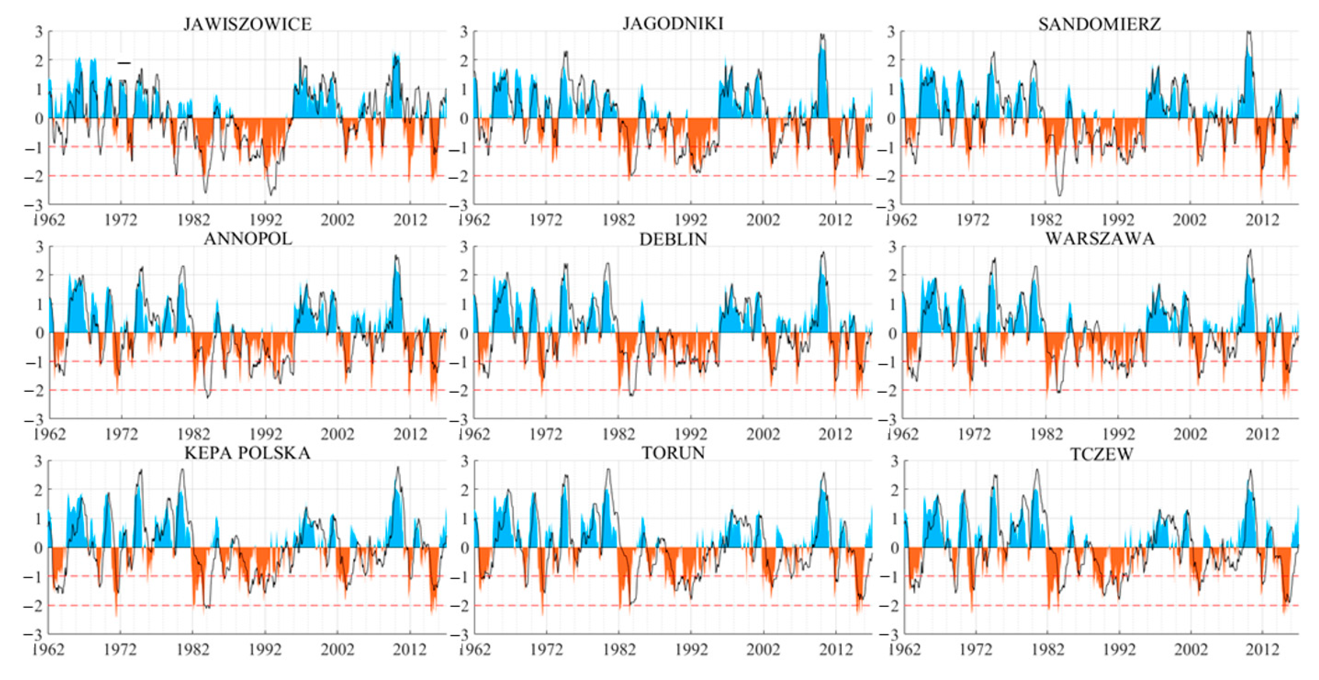
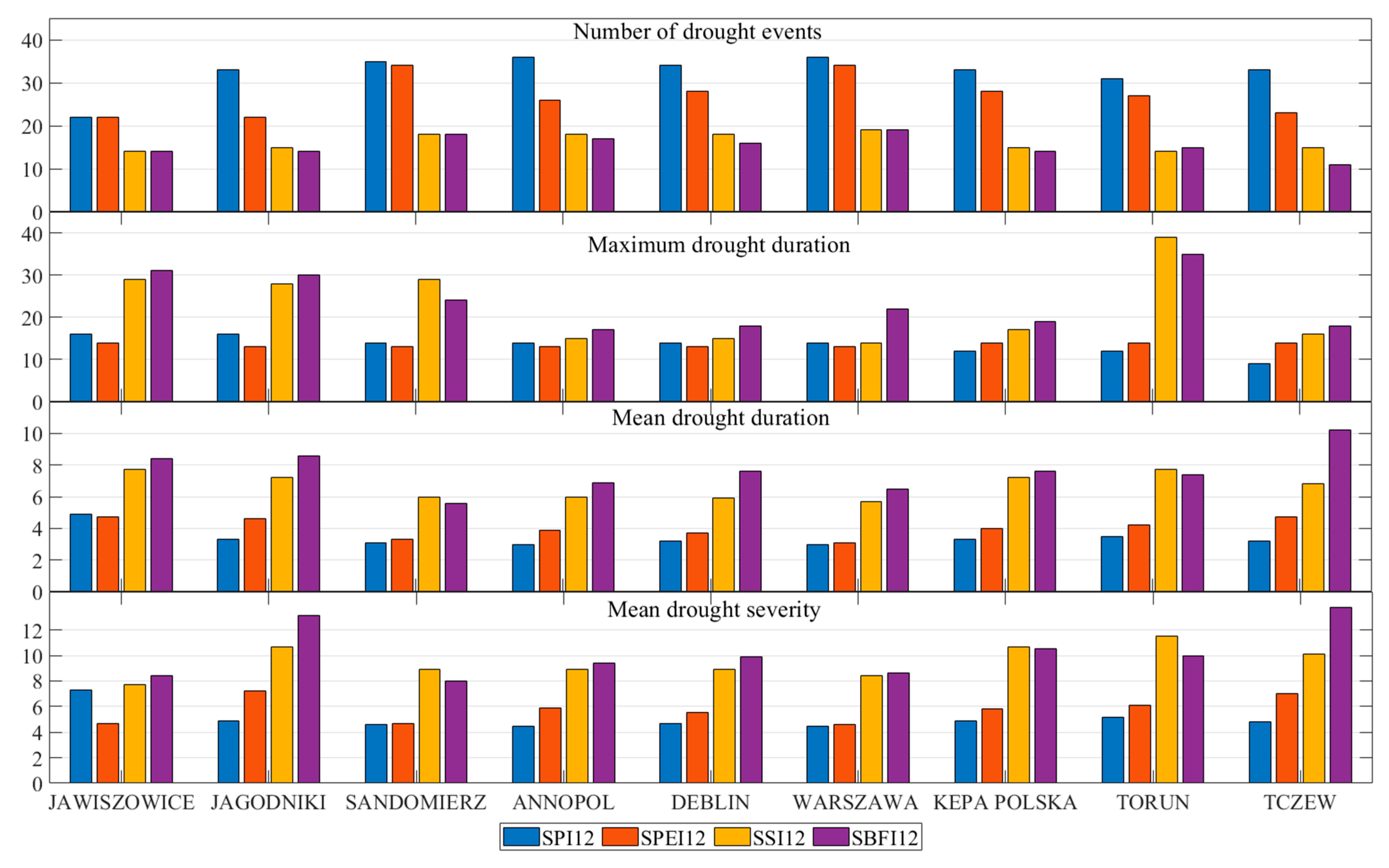
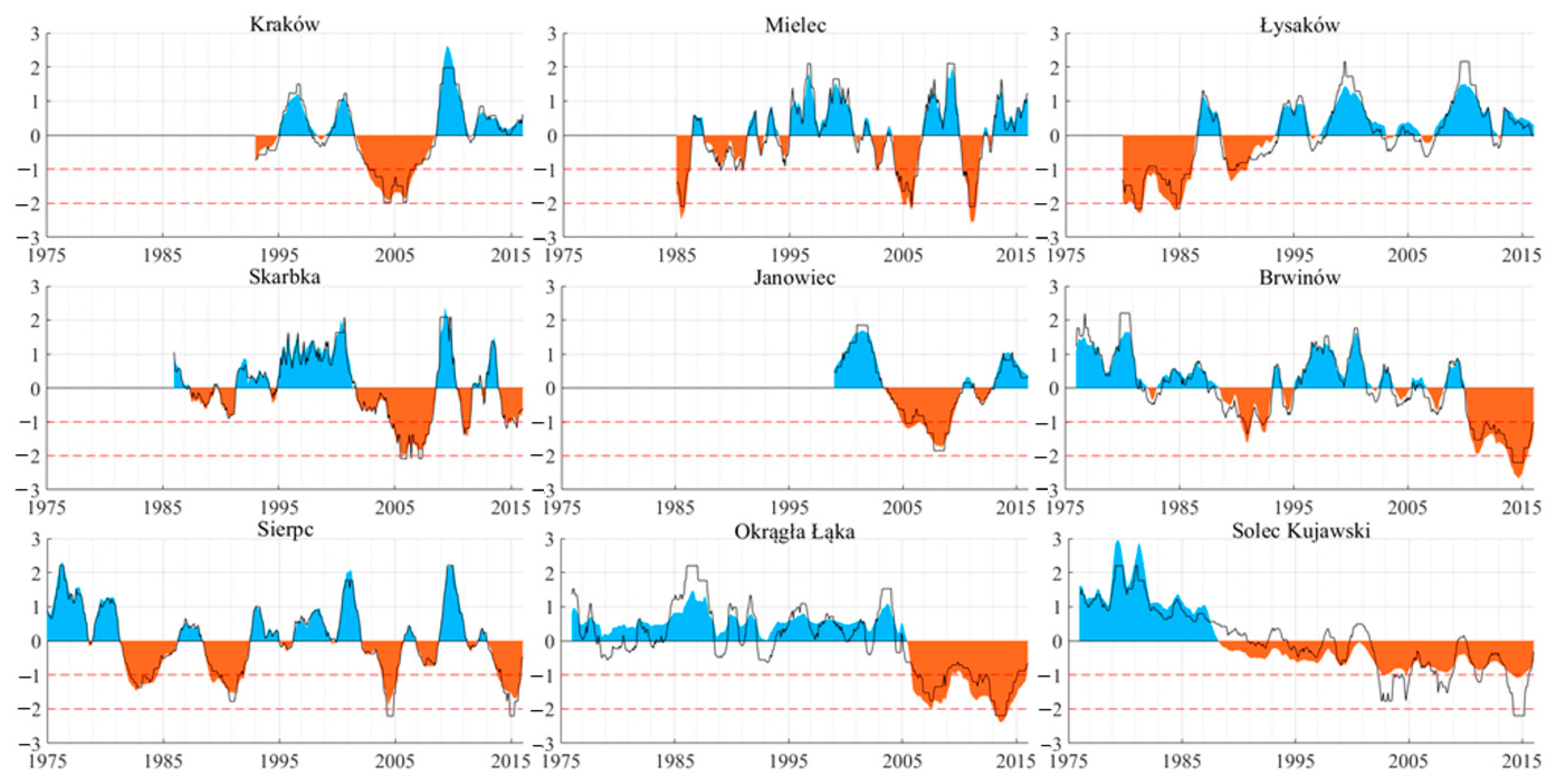
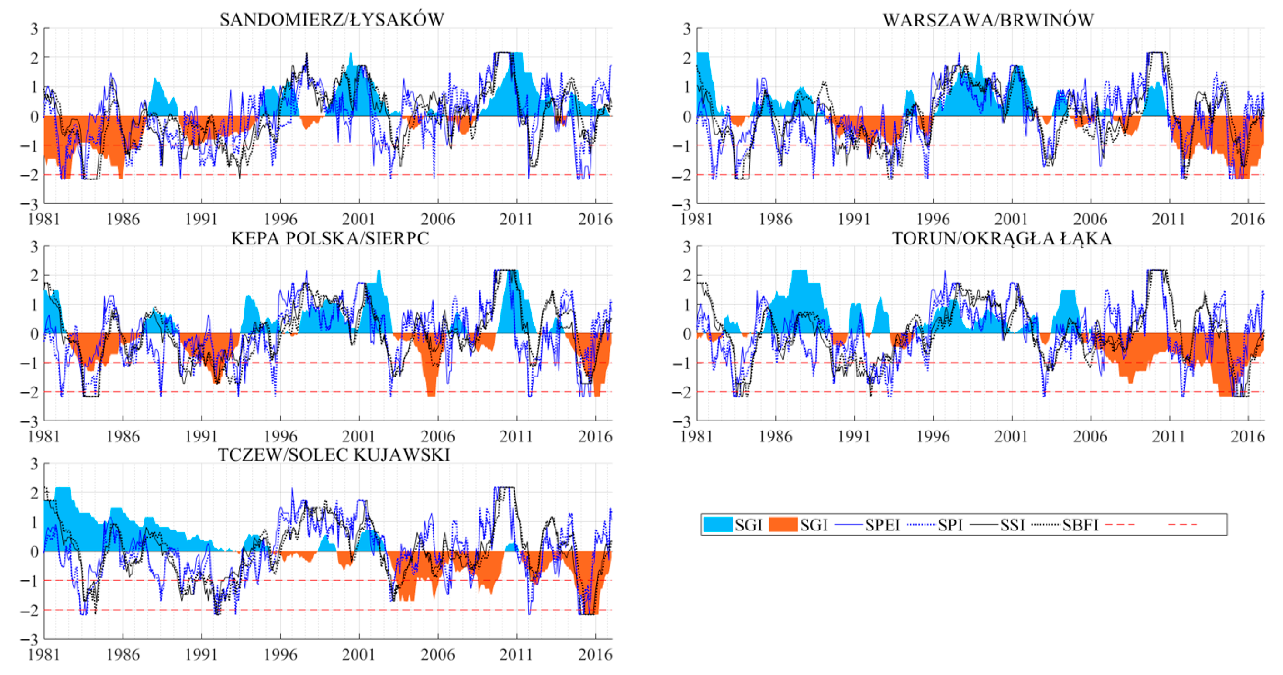
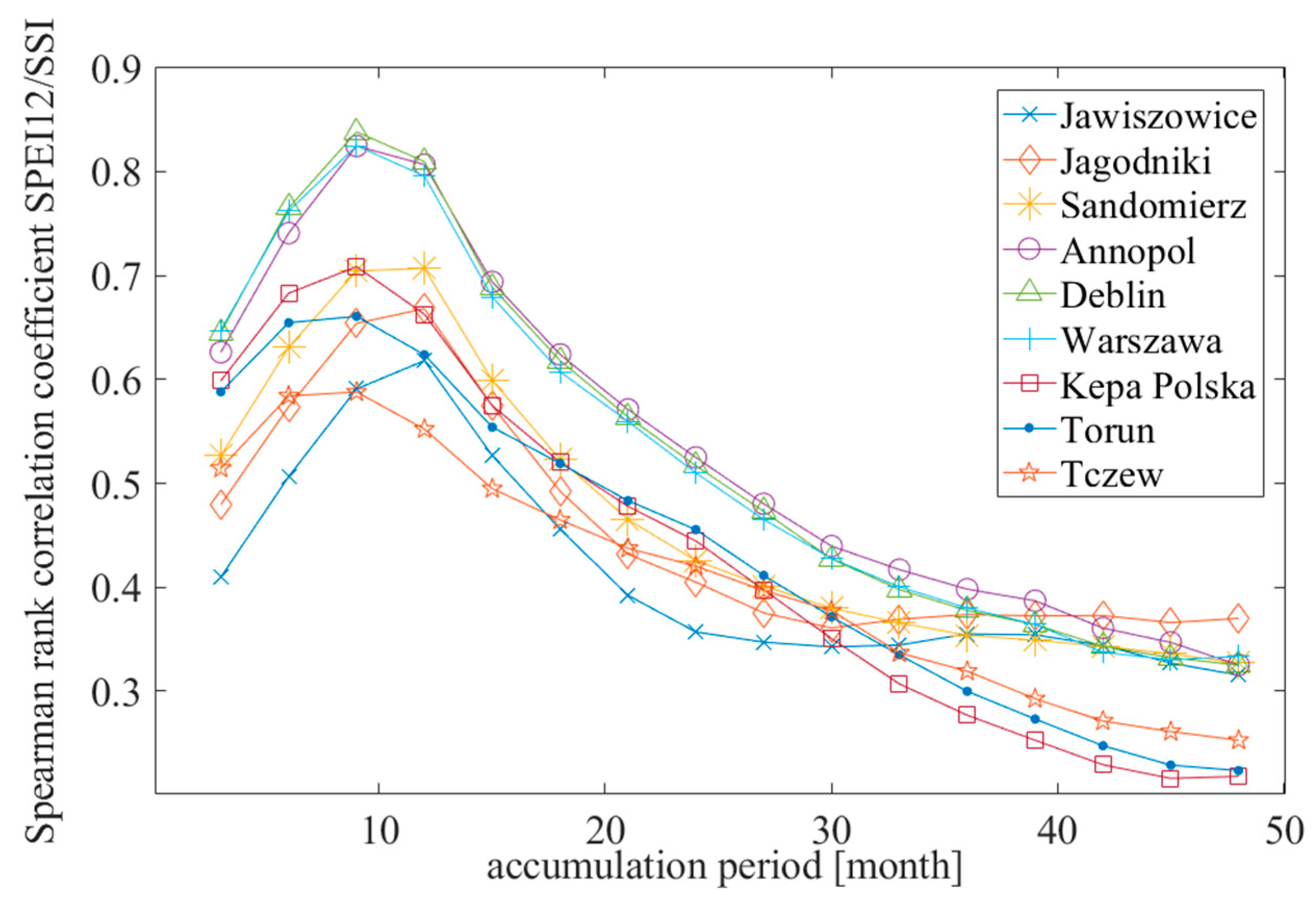
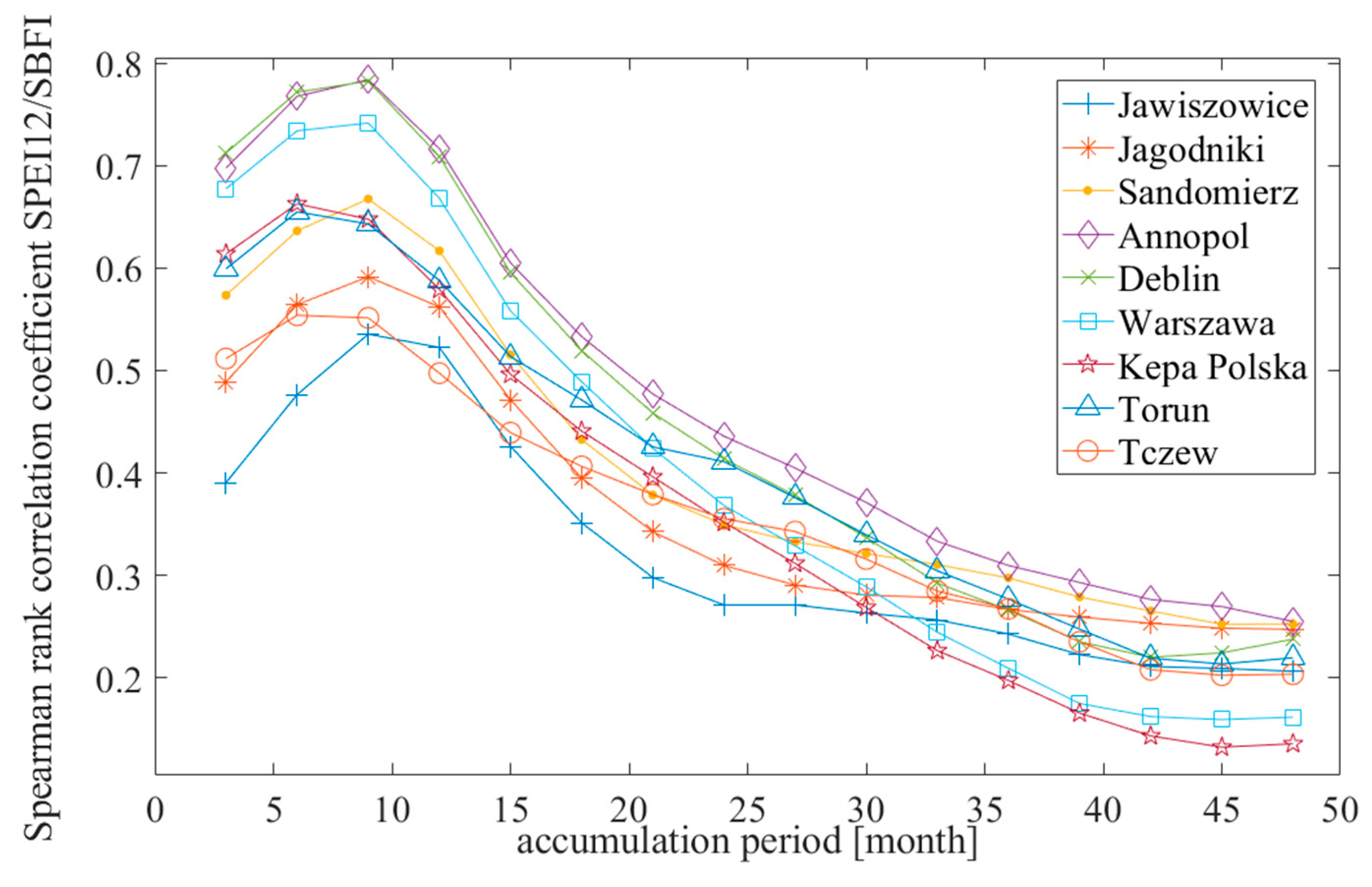
Table 1.
Precipitation characteristics in selected meteorological stations.
| Station | River | Geographical Coordinates | Observation Period | Mean Annual Precipitation (mm) |
|---|---|---|---|---|
| Białystok | Biała | N | 1951–2019 | 594 |
| Bielsko-Biała | Biała | N | 1951–2019 | 989 |
| Kasprowy Wierch | Dunajec | N | 1951–2019 | 1759 |
| Katowice | Rawa | N | 1951–2019 | 714 |
| Tarnów | Dunajec | N | 1951–2019 | 705 |
Table 2.
The list of hydrological stations along the course of the Vistula River used in the study in continuous operation since 1951.
Table 2.
The list of hydrological stations along the course of the Vistula River used in the study in continuous operation since 1951.
| Station | Basin | Basin Area (km2) * | Anthropopression | Types of Water Structures | Remarks |
|---|---|---|---|---|---|
| Jawiszowice | Upper Vistula | 970.6 | Altered | Discharges 1 | |
| Jagodniki | Upper Vistula | 12,058.2 | Altered | Barrages 2 | |
| Sandomierz | Upper Vistula | 31,846.5 | Altered | ||
| Annopol | Middle Vistula | 51,518.1 | Natural | ||
| Dęblin | Middle Vistula | 68,234.3 | Natural | ||
| Warszawa | Middle Vistula | 84,539.5 | Natural | 1968 3 | |
| Kępa Polska | Lower Vistula | 168,956.1 | Natural | 1969 3 | |
| Toruń | Lower Vistula | 181,033.4 | Altered | Barrages 2 | |
| Tczew | Lower Vistula | 193,921.0 | Altered |
Note: 1 mine water, 2 upstream, 3 change in measurement location, * [23].
Table 3.
Available and prospective groundwater resources in the Vistula basin [25].
Table 3.
Available and prospective groundwater resources in the Vistula basin [25].
| Name of Sub-Basin Area | Disposable Resources | Perspective Resources | Total | |||
|---|---|---|---|---|---|---|
| Area (km2) | (103 m3/day) | Area (km2) | (103 m3/day) | Area (km2) | (103 m3/day) | |
| Upper Vistula | 12,940 | 1050.16 | 34,474 | 4605 | 47,414 | 4818 |
| Middle Vistula | 61,343 | 5253.32 | 50,962 | 7209 | 112,305 | 12,463 |
| Lower Vistula | 15,820 | 1747.80 | 18,850 | 2376 | 34,670 | 4124 |
| Vistula Basin | 90,103 | 8041.28 | 104,286 | 14,190 | 194,389 | 22,232 |
Table 4.
Drought categories based on the drought index value.
| Drought Categories | |
|---|---|
| No drought | |
| Normal drought | |
| Moderate drought | |
| Severe drought | |
| Extreme drought |
Table 5.
The characteristics of seasonal and annual flow at selected stations in the 1951–2018 period. HHQ—the highest of the highest flow in the period, MHQ—the mean highest flow; MMQ—the mean flow; MLQ—the mean lowest flow; LLQ the lowest of the lowest flow.
Table 5.
The characteristics of seasonal and annual flow at selected stations in the 1951–2018 period. HHQ—the highest of the highest flow in the period, MHQ—the mean highest flow; MMQ—the mean flow; MLQ—the mean lowest flow; LLQ the lowest of the lowest flow.
| Winter Season (XI–IV) (m3/s) | Summer Season (V–X) (m3/s) | Year (XI–X) (m3/s) | |||||||||||||
|---|---|---|---|---|---|---|---|---|---|---|---|---|---|---|---|
| Station | HHQ | MHQ | MMQ | MLQ | LLQ | HHQ | MHQ | MMQ | MLQ | LLQ | HHQ | MHQ | MMQ | MLQ | LLQ |
| Jawiszowice | 187 | 69.1 | 12.5 | 2.83 | 1.2 | 792 | 153 | 13.5 | 2.46 | 0.95 | 792 | 161 | 13.0 | 2.32 | 0.95 |
| Jagodniki | 1220 | 571 | 130 | 53.1 | 30.2 | 3400 | 960 | 126 | 51.1 | 27.8 | 3400 | 1060 | 128 | 46.7 | 27.8 |
| Sandomierz | 3460 | 1270 | 292 | 109 | 57.0 | 5690 | 1910 | 285 | 109 | 66.6 | 5690 | 2190 | 289 | 94.9 | 57.0 |
| Annopol | 5380 | 1850 | 451 | 163 | 88.2 | 6200 | 2350 | 409 | 163 | 106 | 6200 | 2730 | 430 | 137 | 88.2 |
| Dęblin | 4480 | 1880 | 526 | 203 | 112 | 6000 | 2210 | 465 | 209 | 121 | 6000 | 2640 | 496 | 176 | 112 |
| Warszawa | 5060 | 2050 | 609 | 250 | 108 | 5940 | 2230 | 527 | 261 | 153 | 5940 | 2740 | 568 | 215 | 108 |
| Kępa Polska | 5580 | 3010 | 1050 | 412 | 162 | 6980 | 2570 | 791 | 385 | 234 | 6980 | 3500 | 918 | 333 | 162 |
| Toruń | 5810 | 3110 | 1110 | 405 | 211 | 6890 | 2570 | 833 | 403 | 205 | 6890 | 3530 | 970 | 349 | 205 |
| Tczew | 5960 | 2940 | 1180 | 495 | 264 | 6490 | 2430 | 905 | 485 | 266 | 6490 | 3310 | 1040 | 418 | 264 |
Table 6.
The results of testing (α = 0.05) for trend and change point in seasonal minimum flow (LQ) series in the 1951–2018 period.
Table 6.
The results of testing (α = 0.05) for trend and change point in seasonal minimum flow (LQ) series in the 1951–2018 period.
| Station | Mann Test for Trend LQ | Pettitt Test for Change Point Detection, LQ | ||||
|---|---|---|---|---|---|---|
| Winter | Summer | Winter | Summer | Change Point (Winter) | Change Point (Summer) | |
| Jawiszowice | NS | NS | NS | NS | - | - |
| Jagodniki | NS | NS | SPS | SPS | 1966 | 1989 |
| Sandomierz | SP | NS | SPS | NS | 1970 | - |
| Annopol | NS | NS | NS | NS | - | - |
| Dęblin | NS | NS | NS | NS | - | - |
| Warszawa | SP | NS | SPS | NS | 1974 | - |
| Kępa Polska | NS | NS | SPS | NS | 1966 | - |
| Toruń | NS | SN | NS | SNS | - | 1989 |
| Tczew | NS | NS | NS | NS | - | - |
Note. NS = non-significant, SP = significant positive, SN = significant negative, SPS = significant positive shift, SNS = significant negative shift, LQ = minimum flow.
Table 7.
The results of testing (α = 0.05) for trend and change point in annual minimum flow (LQ) series in the 1951–2018 period.
Table 7.
The results of testing (α = 0.05) for trend and change point in annual minimum flow (LQ) series in the 1951–2018 period.
| Station | Mann Test for Trend | Pettitt Test for Change-Point Detection | |
|---|---|---|---|
| LQ (Annual) | LQ (Annual) | Change Point (Annual) | |
| Jawiszowice | NS | NS | - |
| Jagodniki | NS | SPS | 1964 |
| Sandomierz | SP | SPS | 1964 |
| Annopol | NS | SPS | 1964 |
| Dęblin | SP | SPS | 1964 |
| Warszawa | SP | SPS | 1974 |
| Kępa Polska | NS | SPS | 1973 |
| Toruń | NS | NS | - |
| Tczew | NS | NS | - |
Note. NS = non-significant, SP = significant positive, SPS = significant positive shift, LQ = minimum flow.
Publisher’s Note: MDPI stays neutral with regard to jurisdictional claims in published maps and institutional affiliations. |
© 2021 by the authors. Licensee MDPI, Basel, Switzerland. This article is an open access article distributed under the terms and conditions of the Creative Commons Attribution (CC BY) license (http://creativecommons.org/licenses/by/4.0/).
Share and Cite
MDPI and ACS Style
Karamuz, E.; Bogdanowicz, E.; Senbeta, T.B.; Napiórkowski, J.J.; Romanowicz, R.J. Is It a Drought or Only a Fluctuation in Precipitation Patterns?—Drought Reconnaissance in Poland. Water 2021, 13, 807. https://doi.org/10.3390/w13060807
AMA Style
Karamuz E, Bogdanowicz E, Senbeta TB, Napiórkowski JJ, Romanowicz RJ. Is It a Drought or Only a Fluctuation in Precipitation Patterns?—Drought Reconnaissance in Poland. Water. 2021; 13(6):807. https://doi.org/10.3390/w13060807
Chicago/Turabian StyleKaramuz, Emilia, Ewa Bogdanowicz, Tesfaye Belay Senbeta, Jarosław Jan Napiórkowski, and Renata Julita Romanowicz. 2021. "Is It a Drought or Only a Fluctuation in Precipitation Patterns?—Drought Reconnaissance in Poland" Water 13, no. 6: 807. https://doi.org/10.3390/w13060807
Note that from the first issue of 2016, this journal uses article numbers instead of page numbers. See further details here.