Sea Topography of the Ionian and Adriatic Seas Using Repeated GNSS Measurements

Abstract

The mean sea surface topography of the Ionian and Adriatic Seas has been determined. This was based on six-months of Global Navigation Satellite System (GNSS) measurements which were performed on the Ionian Queen (a ship). The measurements were analyzed following a double-path methodology based on differential GNSS (D-GNSS) and precise point positioning (PPP) analysis. Numerical filtering techniques, multi-parametric accuracy analysis and a new technique for removing the meteorological tide factors were also used. Results were compared with the EGM96 geoid model. The calculated differences ranged between 0 and 48 cm. The error of the results was estimated to fall within 3.31 cm. The 3D image of the marine topography in the region shows a nearly constant slope of 4 cm/km in the N–S direction. Thus, the effectiveness of the approach “repeated GNSS measurements on the same route of a ship” developed in the context of “GNSS methods on floating means” has been demonstrated. The application of this approach using systematic multi-track recordings on conventional liner ships is very promising, as it may open possibilities for widespread use of the methodology across the world.

1. Introduction

For many years the precise determination of the geoid has been one of the basic problems of physical geodesy. The geoid is the equipotential surface that describes the irregular shape of the Earth and is used as the zero reference for elevation measurements. This would coincide with the Mean Sea Level (MSL), provided that dynamic factors (wind, atmospheric pressure, tide, sea currents, etc.) were to be excluded—that is, if oceans and atmosphere were to be considered in equilibrium. If we extended the MSL below the continents by means of hypothetical canals, we could obtain the whole image of the geoid surface. The precise knowledge of the geoid is very important in several applications, e.g., in investigating petroleum deposits. It is worth noting that the altitudes on the geoid are estimated with respect to the ellipsoid Earth. The methods for determining the geoid can be classified into indirect and direct ones.

Traditionally, the geoid has been determined indirectly either by gravitational or by astro-geodetic measurements in combination with various mathematical transformations (such as the Stokes equations). However, these calculations involve a great amount of uncertainty that can be up to several meters.

The more recent direct methods for geoid determination include marine surface measurements by altimetry satellites [1] and airplane laser scanners [2], and “GNSS on floating means” measurements [3]. The first two methods face double uncertainty, since the calculation of the Global Navigation Satellite System (GNSS) position is required in addition to the distance estimation of the altimetry satellite or plane from the sea surface. Furthermore, they face significant problems in coastal areas and closed seas due to land obstacles. To address these problems, a new method based on direct GNSS measurement on the surface of the sea has been developed. During the decade 2003–2013, a number of research groups have proposed “on-ship” GNSS measurements for the determination of sea surface topography, contributing to the development of this method [4,5,6,7,8,9,10,11,12,13,14].

The installation of one or more GPS/GNSS receivers on a navigable medium was based on earlier research efforts involving GPS/GNSS placement on a buoy [15,16,17]. These buoys used GPS/GNSS to measure the dynamic characteristics of the waves and the average sea level of a particular point. Thus, the topography of a marine area could not be assessed. The GPS/GNSS buoy methodology was developed mainly for the construction of early tsunami warning systems [18,19].

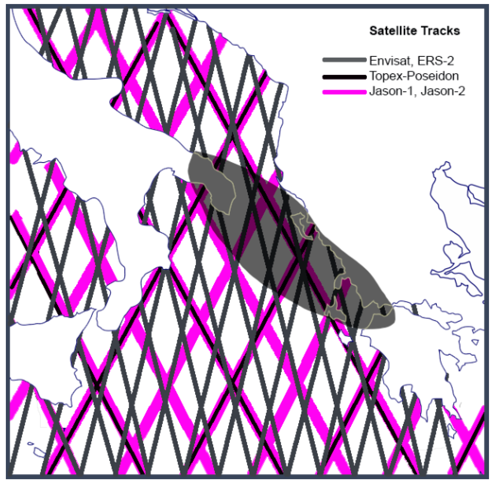
The goal of this work was the determination of the mean surface topography (MST) of the Ionian and Adriatic Seas. This was attempted by developing an alternative methodology in the context of the “GNSS on floating means” techniques. The methodology followed in the present work is highly promising for various reasons. Firstly, the exact knowledge of the shape of the sea surface may provide quite useful information concerning climate change. It is well known that in most cases the investigation concerning the effect of global warming on the sea level is limited to certain places of the coast, where tide gauges are installed [20]. However, this approach does not allow investigating the important effects of global warming on the shape of the sea surface. Those effects, to the extent of the author’s knowledge, remain for the moment largely unknown. This issue could be investigated through studies like the present one, repeated at regular intervals. Secondly, an obvious advantage of the present method with respect to the methods based on altimeter satellites is that the hundreds of thousands of passenger and cargo ships traveling worldwide provide a continuous grid of potential measurements. It is actually simpler to place a GNSS on a ship than to launch an altimeter satellite. Moreover, the satellites measure the sea surface at specific points, only along their orbit (Figure 1), whereas the method “GNSS on ship” allows one to identify possible small changes or anomalies anywhere on the sea surface and to focus at specific points not covered by satellites. Furthermore, the methods based on satellites fail to provide good accuracy in coastal areas [21]. In these areas, however, the determination of the average marine topography and the geoid is of great scientific interest [22]. The detection of significant changes in specific parts of the marine topography could reveal interesting geological structures of the marine subsoil related to fissures or oil and gas fields [23]. This perspective is very important, especially for the study area, because it presents very high seismicity but also strong indications for the existence of hydrocarbon deposits [24].

The region under consideration extends from the Gulf of Patras to the northern Ionian Sea and the southern Adriatic Sea up to the port of Brindisi. It covers 250 km north–south and 150 to 200 km east–west. A schematic representation of the region studied is illustrated in Figure 1 (red region) together with the trajectories of the TOPEX/POSEIDON, Jason-1, Jason-2, Envisat and ERS-2 satellites in the eastern Mediterranean region.

The mean sea level in the region studied, approached satisfactorily by the estimates of the geoid, has changed considerably, creating differences in height of several meters, in some cases larger than 10 m. For example, the EGM96 model estimates a sea level in the area near to the port of Brindisi as 14.2 m higher than that estimated in the sea area near the port of Patras, with respect to the ellipsoid reference [25]. The study of surface sea surveying in the above area following the new approach is of interest for several reasons. Specifically, the few tide recording stations do not allow developing a clear picture concerning the eventual changes in sea level due to medium-term meteorological factors or to even more permanent fluctuations due to climate change. Thus, in many cases we cannot know whether the sinking or rising shores observed in the area are due to geological causes, meteorological fluctuations or both. Additionally, the trajectories of the TOPEX/POSEIDON, Jason-1, Jason-2, Envisat and ERS-2 altimetry satellite missions intersect over the area studied (Figure 1, red). However, the estimates of altitude satellites are subject to significant uncertainties ranging from five to ten centimeters in the assessment of marine topography near coastal areas or areas with extensive coastline [26].

Although the idea of placing a GNSS receiver on a passenger ship for recording a single track has been suggested [8], the technique presents significant weaknesses as far as the uncertainties are concerned [3]. Developing an approach of repeated measurements on the same route offers the potential of significantly reducing uncertainties and improving the methodology. Thus, the main approach of the present contribution is to carry out multiple measurements (passes) for the same maritime route over several months in order to include all possible conditions. Adopting this approach is expected to lead to higher accuracy estimations for marine topography, especially when compared with older methodologies. In the present work we have used the “Patra – Igoumenitsa – Brindisi” line for developing our methodology, using measurements from the “Ionian Queen” passenger ship over a period of 6 months. Using our method, we studied the change of the sea level altitude along the ship’s route, to determine the sea surface topography and compare our estimates to those of the geoid EGM96 model.

Two alternative methods were used to resolve our data, differential GNSS (D-GNSS) and precise point positioning (PPP). The main difference between these methods is that the first one requires a fixed GNSS reference station at a short distance from the moving receiver, in order to remove the atmospheric noise from the data [27]. This fixed station must be on land. The greater the distance from land, the poorer the accuracy. Thus, despite the fact that the D-GNSS method potentially provides data with much higher accuracy than any other method [28], its use away from the shore is quite problematic. On the contrary, the PPP method does not require a fixed station and is ideal for marine topography. However, its accuracy still remains lower than D-GNSS, though it is constantly improving [29]. In the present work, a combination of both methods was adopted, to constitute a model approach for studying marine topography.

2. Experimental Measurements

2.1. GNSS Records on the Boat

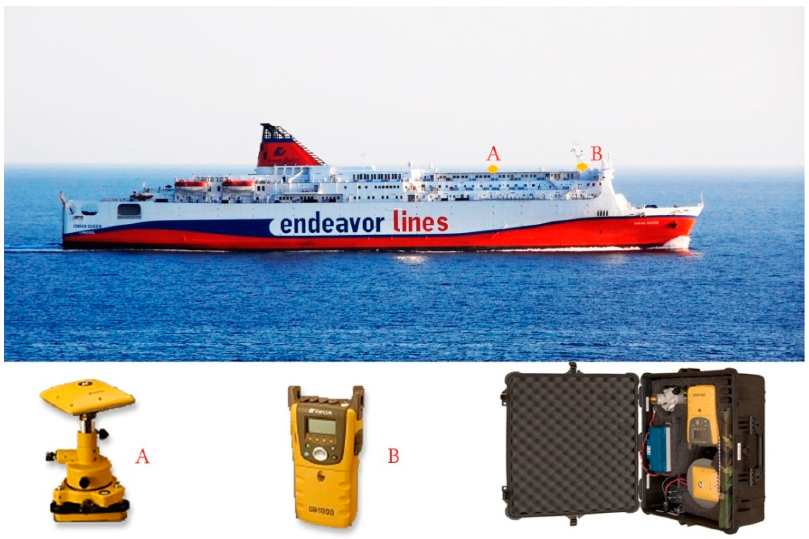
The ship utilized was the “Ionian Queen of Endeavor Lines.” The GNSS receiver (GB-1000 from Topcon with PG-A1 antenna) was placed in a suitable position on the ship’s deck for decreasing the multi-reflection effect. Figure 2 shows the locations of the receiver antenna (A) and the receiver (B)—which was located inside a watertight suitcase used for its protection. The records concern the period from 30 January to 20 July 2010 and involved 142 passes. These were recorded at a sampling rate of 1 Hz and a circumferential angle of 15 degrees, which protected the GNSS receiver from any side obstacles.

Information concerning the 142 routes is compiled in Table S1. Each route (code number ID) concerns a separate voyage of the ship from Patras to Brindisi or vice versa. The data were analyzed using two methods (D-GNSS [30] and PPP [31]). In some cases, uncertainties in the frame of D-GNSS and some error reports when solving with PPP could not be resolved. Thus, some of these routes were not finally utilized for the assessment of marine topography. As shown in Table S1, data from 127 and 121 routes were utilized, respectively, in the context D-GNSS and PPP.

2.2. Ship Depth Altimeter Data

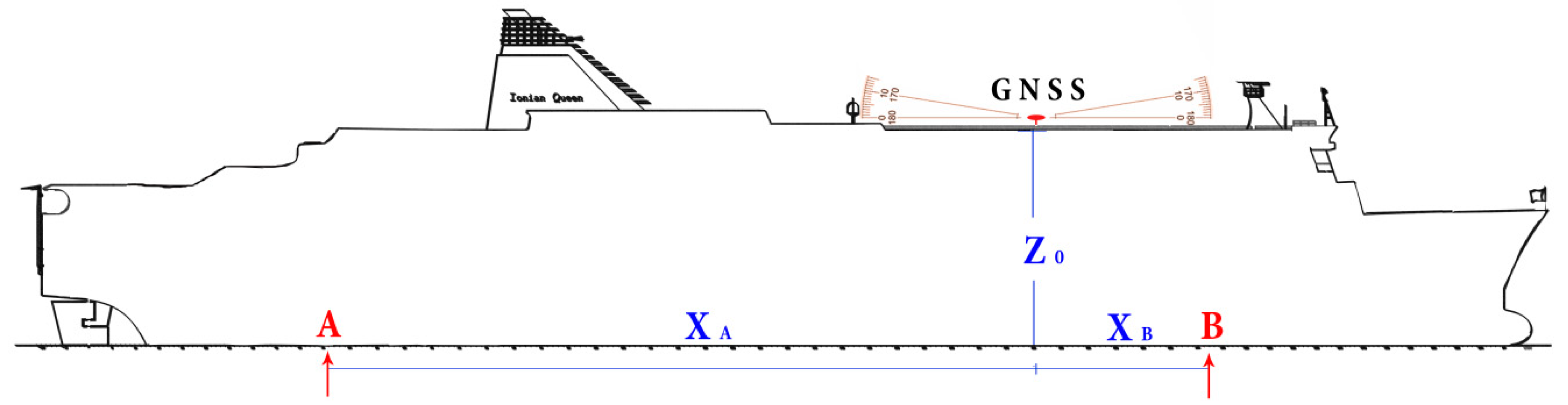
Α systematic recording of the ship’s elevation was performed at two points of the ship (bow (B) and stern (A)) along with the collection of the GNSS records. These points are illustrated in Figure 3. The altitudes were recorded by the ship’s crew at each of the port stations of the route (Patras–Igoumenitsa–Brindisi). Due to the ship’s loading and unloading, the draughts were taken by the crew just prior to departure and after the ship had been fully loaded. Devices calculating the draught at points A and B were permanent ship equipment and operated—according to their specifications—with a precision of 1 cm. The received draught data were used for determining accurately the distance of the receiver from the surface of the sea. Table S2 illustrates indicative data concerning the ship’s draughts (h_Α and h_Β) at points A and B.

2.3. Data from Permanent GNSS Stations

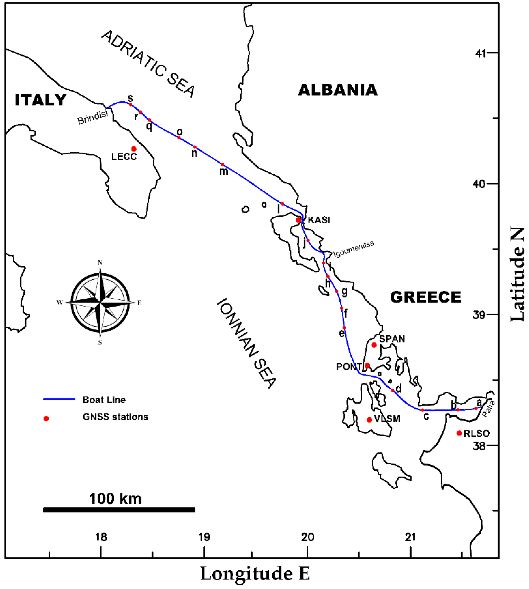
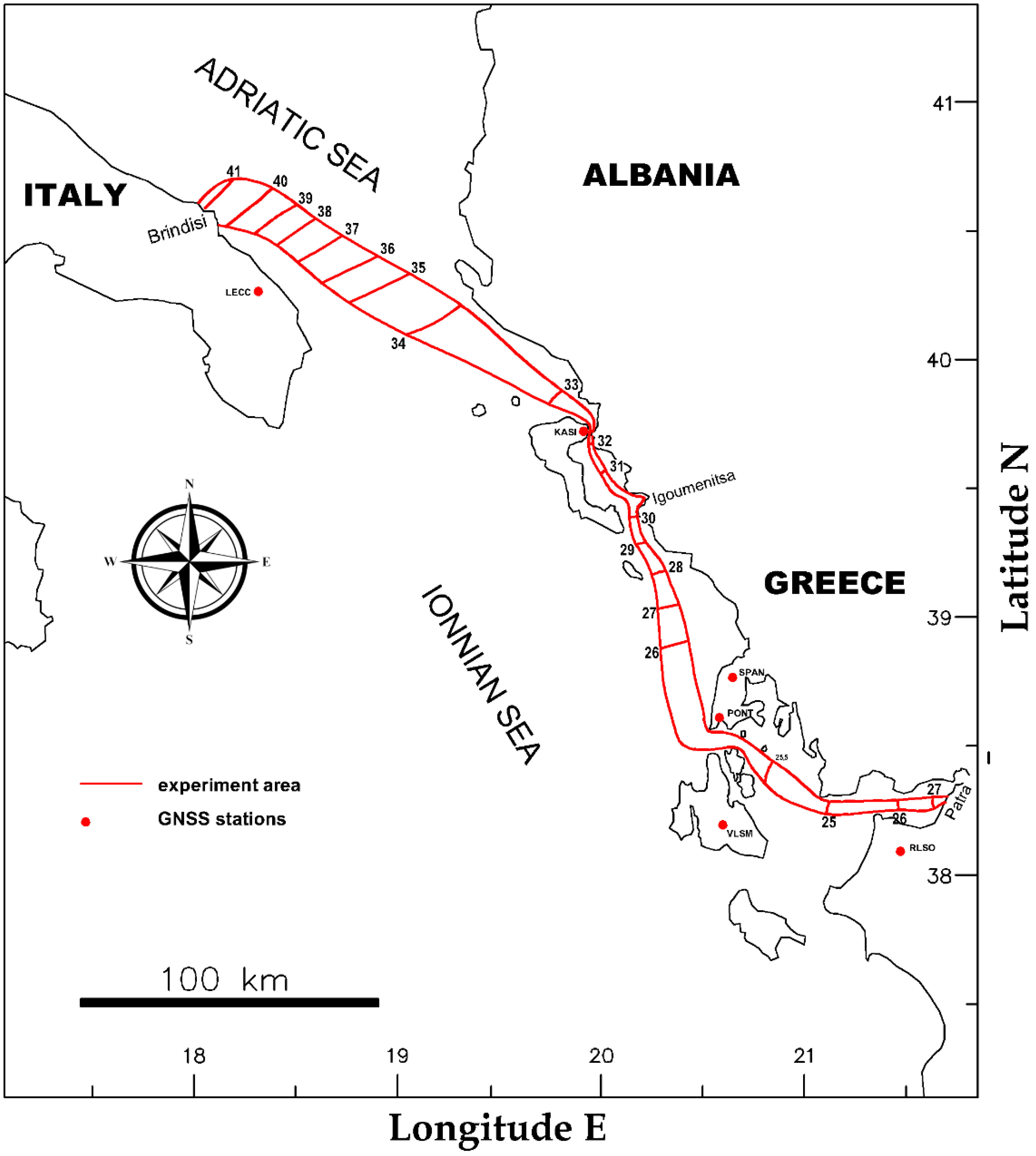
Data from permanent GNSS stations in Greece and Italy were also collected, in addition to those collected by the GNSS on the boat. The locations of the recording stations are shown in Figure 4.

These stations were tested due to their proximity to segments of the ship’s seaway, in order to be used as reference stations when resolving with the D-GNSS method. The networks utilized provide free data compatible with the resolution methods we have chosen. Moreover, the stations were recording during the marine experiments and provided data with a sampling period of 15 and/or 30 s.

3. Methodology

3.1. General Procedure for Calculating the Mean Sea Level (MSL)

The calculation of the sea altitudes is inevitably quite complex because it is based on multiple crossings for marine topography. The ultimate goal of the analysis of the time series which were received from the GNSS solutions was the determination of the mean sea level (MSL). In this section the methodology for calculating the MSL using GNSS receiver’s altitude measured at each moment is presented and analyzed.

For each separate route, the measured geometric altitude H (i,t) of the receiver on the ship at time t and position i is defined by the equation:

$$H\left(i,t\right)=\Psi \left(i\right)-h_{GNSS}\left(i,t\right)\pm h_{wave}\left(i,t\right)\pm h_{tide}\left(i,t\right)\pm u\left(i,t\right),$$

(1)

where

$h_{GNSS}\left(i,t\right)$: The height of the receiver relative to the sea surface.

$h_{tide}\left(i,t\right)$: The effect of astronomical and meteorological tide.

$$h_{tide}\left(i,t\right)=h_{astro}\left(i,t\right)+h_{meteo}\left(i,t\right)$$

(2)

$h_{wave}\left(i,t\right)$: The effect of waves.

$u\left(i,t\right)$: The total error of the measurement (random and systematic) of the geometric altitude of the receiver$,H\left(i,t\right)$.

$\Psi \left(i\right)$: The requested (unknown) geometric altitude of the MSL at position i.

The above parameters refer to a position i at time t.

Figure 5 shows a schematic representation of the main parameters of Equation (1). It should be noted again that the parameter H(t,i) is deduced from the GNSS recordings, whereas the parameter h_GNSS is calculated by means of geometric characteristics of the ships taking into account the draught of the ship. Moreover, the estimations of the effects of astronomical and meteorological factors of the tide were based on GNSS measurements in ports and static solutions in order to determine the geometric altitude H (i,t) in ports.

The determination of all parameters of Equation (1) and the estimation of their uncertainties allows approaching the desired altitude Ψ(i) together with its precision. This can be done for each route separately. The contribution of the present approach, however, is that it uses multiple paths and thus it can determine altitudes Ψ(i) more accurately than methods using single paths. To calculate a reliable altitude at each point Ψ(i) for each of the aforementioned parameters of Equation (1), we should into account the uncertainties which can affect the final results. For the calculation of these parameters, a step-by-step analysis was followed, which is described in the next sections. Starting with the parameter h_GNSS, it was calculated by means of the geometric characteristics of the ships and corrected by taking into account the draught of the ship (Section 3.2). Continuing, the impact of astronomical tide, the meteorological factor of the tide and the estimation of the effect of waves (Section 3.3) are presented. Finally, we are presenting our methodology relevant to the solution of the GNSS raw data for determining the H(i,t) values, following the differential GNSS (D-GNSS; Section 3.4) and precise point positioning (PPP; Section 3.5) methods.

Before the next subsections, it is important to note that the multiple-paths approach developed in this work had to address the following methodological problem: The ship, on each separate route, although driven by an automatic satellite navigation system (using GNSS), does not always follow an identical route. It deviates in the horizontal plane. Figure 6 illustrates an indicative area, near to the port of Brindisi, with nine different crossings. It is seen that the different routes, although somewhat parallel, may vary by tens of meters. The deviation may be even greater. An example is illustrated in Figure S1. It concerns eight different routes (11/2–19/2, route IDs 13–21, Table S1). In view of the above for determining the altitude H (i,t), we cannot use a point on an individual route (e.g., route 1, Figure 6), but instead must use a “mean point” on the straight section that intersects almost vertically all the different paths at corresponding points. These “mean points” constitute the “principal path” illustrated in Figure 4. It is important to note that the differences in the values of H (i,t) determined at these corresponding points are actually negligible, and this allows us to draw conclusions for a broader zone around the “principal route.”

3.2. Correction of the Altitude of the Receiver Relative to the Sea Level (h_GNSS) to Take into Account the Cargo Changes after Each Loading and Unloading of the Ship

As already mentioned, the GNSS receiver was stationary on the ship (Figure 3). However, its altitude in relation to the sea level (light blue in Figure 5) was changed at each port due to cargo changes after each loading and unloading. This required a suitable correction for each route.

The recordings of the draughts at positions A and B (Table S2) were adjusted by means of a simple linear interpolation at the projection point of the GNSS receiver (see Figure 3) according to the equation:

$$h_{GNSS}=Z_0-H_s=Z_0-\left[x_a\frac{\left(h_b-h_a\right)}{\left(x_a+x_b\right)}\right]+h_a$$

(3)

where$h_{GNSS}$ is the requested height of the receiver relative to the sea surface; $Z_0$ is the known height of the receiver relative to the ship’s bottom level horizontal keel;$h_a,h_{\beta }$ is the measured ship draughts at control points A and B (see Figure 3);$x_a$ and $x_{\beta }$are horizontal distances from the A and B points of the depth-meters in relation to the projection point of the GNSS receiver on the AB section of the horizontal keel;$H_s$ is the draught altitude at the intersection point corresponding to the projection point of the GNSS receiver on the AB section of the horizontal keel.

Figure 7 illustrates the geometric calculation of the antenna height relative to the plane of the sea surface.

Based on the accuracy of the A and B draught measurements, as provided by the ship’s instrument specifications, the error of the determined parameter h_GNSS has been estimated. The calculations are presented in Appendix A and resulted to an error equal to 0.76589 cm.

3.3. Calculation of Impact of Astronomical Tide and Meteorological Factor of the Tide, h_tide: Static Calculation of Altitude in Ports

The determination of the impacts of the astronomical and meteorological factors of the tide, $h_{tide}$, on the requested parameter, Ψ(i), allows removing their influence. To determine such an impact, we used to a static solution in the ports. The ship remained each day in the ports of Patras or Brindisi for a period of 4 h and this allowed solving statically the altitudes in all cases. The time period chosen for resolution (2.5 h) was less than 4 h in order to correspond to the time that the ship was completely empty and not in the process of loading or unloading. Taking into account the magnitude of the tide and the rate of its change in the area [32] we considered that at this period the sea level remained constant, and thus a static solution could provide a reliable estimate of the altitude of the sea level in ports. The static solution of altitude in ports was performed following the PPP methodology. Figure 8 illustrates the results of the static resolutions in both ports. The mean values and the standard deviation values are also illustrated. Representative results are also illustrated in Table S3.

Since our measurements cover almost one full semester, and they take into account all possible weather conditions, which justifies the variations observed, we considered that the average sea level altitude (mean values in Figure 8) is an estimate of the MSL in the ports (see Figure 5). Thus, we have obtained two points of “control and correction” in the two ports that are the “extremes” of each route. The obtained MSL values and the individual values resulted from the static resolutions at both ports, and were used in order to correct the altitude estimation curves for each route (linear correction). Essentially, the effect of the tide, h (i,t), was eliminated without using data from the tide gauges, given that they were not in operation. After this correction, our differential resolutions did not show any significant differences at a given point (i) for different routes.

Recently, in 2017, we had the opportunity to confirm the aforementioned mean sea level at the port of Patra. In effect, navy services provided us the opportunity to calculate the coordinates of the benchmark GNSS. The elevation of the benchmark was linked to the sea-level recorder—which during our experiments was, unfortunately, out of order. However, the recent measurements have confirmed our calculation for the average value of sea topography at the port of Patras. This demonstrates the accuracy of the above described methodology for obtaining the mean sea level using the GNSS of the ship.

To confirm twice the static GNSS results above, our estimates of the sea level altitude in the ports were compared with the estimates of the DTU10 global ocean tide model. Tide model estimates are usually preferred but have the disadvantage of being indirect estimations of the sea level altitude. The DTU10 model’s differences from the estimations of our GNSS measurements were very small (<16 cm), except for three cases where the difference was greater, and those routes were removed. These differences can be considered negligible, if we consider that the estimated accuracy of the model is about 20–25 cm [33].

Since the calculations of the impacts of the astronomical and meteorological components of tide were not done using modern time-series via tidal collectors, but using the limit values measured at ports, the uncertainty of this factor cannot be accurately estimated. However, the basic component of the astronomical tide (M2) expected in the area does not exceed a maximum range of 5–7 cm [34]. Therefore, it seems plausible to assume that the astronomical tide is eliminated to such an extent so that its effect is not actually detectable. If, for example, despite the aforementioned linear correction, in some segments of the path, e.g., in the middle section, the astronomical tide adds or removes 1–2 cm from our estimation, it is very difficult to be detected. This is because the uncertainty estimated of each separate route covers this range. In other words, the astronomical component cannot contribute beyond this range.

In our previous works we examined in detail the relationship between meteorological and astronomical tides in some parts of the Mediterranean [35]. The ratio of meteorological to astronomical tides in these areas is very high (up to 40). This makes the effect of the astronomical factor practically insignificant [36]. At the same time, the most important meteorological factor in terms of its effect on the average sea level is completely random [37].

In contrast, the meteorological component of tide is related too much wider ranges than those of the astronomical component; in extreme conditions up to 50 cm [32]. However, the change of its amplitude per time unit is much smoother. Thus, the aforementioned linear correction is sufficient to confront the meteorological component of the tide. Obviously, the presence of noise cannot be excluded. However, the use of data of a 6-month period, during which almost all weather conditions occur, randomizes any uncertainty.

Finally, a few sentences concerning the effect of waves (h_wave): Reinking et al. [8], faced with a problem similar to that of the present work, analyzed the dynamics of a ship with a similar size to the “Ionian Queen.” Although their work concerned a marine area with worse wave conditions (the Atlantic Ocean), the authors concluded that the dynamic movement of the ship is not actually affected by the vertical component of the gravitational ripple. Thus, the negligible displacement of a ship of the magnitude of “Ionian Queen” almost eliminates the effect of small-scale waves. Moreover, taking into account that our data cover a period of almost six months and more than 140 passes, as well as the high frequency of sampling on each route (1 Hz), it seems plausible to assume that the effect of the gravitational wave is zero, as it is randomized.

3.4. Solution of the GNSS Raw Data for Determining the H(i, t) Values Following the D-GNSS Method

The data obtained from the GNSS recordings were classified into separate routes illustrated in Table S1. Each route corresponds to a passage of the ship in the line Patra–Igoumenitsa–Brindisi or Brindisi–Igoumenitsa–Patra. These 142 routes were solved by all six reference stations (Figure 4). However, fifteen routes were not used because they could not be resolved by the base stations, as they showed unresolved uncertainties. Moreover, seven additional routes cannot be solved by the LECC station. Thus, 120 of the 142 routes were finally utilized. For improving the accuracy of the results, a static solution of the six reference stations and a correction of their coordinates were completed prior to carrying out the kinematic solution. Figure 9 depicts the horizontal coordinates of the ship’s principal route as solved by the PONT-based D-GNSS method (see also Figure 4).

The solutions were calculated using Leica Geo Office software (LGO). In order to confront the signal distortion due to the atmospheric delay and take into account the large length of the maritime route, a suitable ionospheric model was automatically adopted by the software. This was based on the updates of the orbital satellite corrections. A full ambiguity-fixed solution was chosen. Since the recordings of our data exceeded 45 min, the calculation of the ionospheric model was chosen from the LGO software. This option has the advantage that the calculations of the model are consistent with the particular conditions prevailing in the region. The software’s ability to calculate the troposphere model was also utilized. This option calculates variations of troposphere delay between the moving and the reference receivers. Different solutions were tested with respect to the degree of resolution of their uncertainties, and those segments in which the uncertainties had not been resolved were rejected.

The distances between the six reference stations range from a few to several hundred kilometers from the ship’s crossing points. According to the literature, the distances of the recording points from the reference stations in the D-GNSS method should not be greater than 50 km, though calculations have shown that a distance of 60 km does not lead to additional uncertainty greater than 2 cm [38]. At higher distances, the noise may become quite large. This is exemplified in Figure S2. It concerns an area in Patra Bay where the data have been resolved by different stations. It is obvious that the noise level increases with the distance of the station from the region mentioned. However, it does not exceed 5 cm. The aforementioned effect of distance is more clearly illustrated in the examples shown in Figure 10.

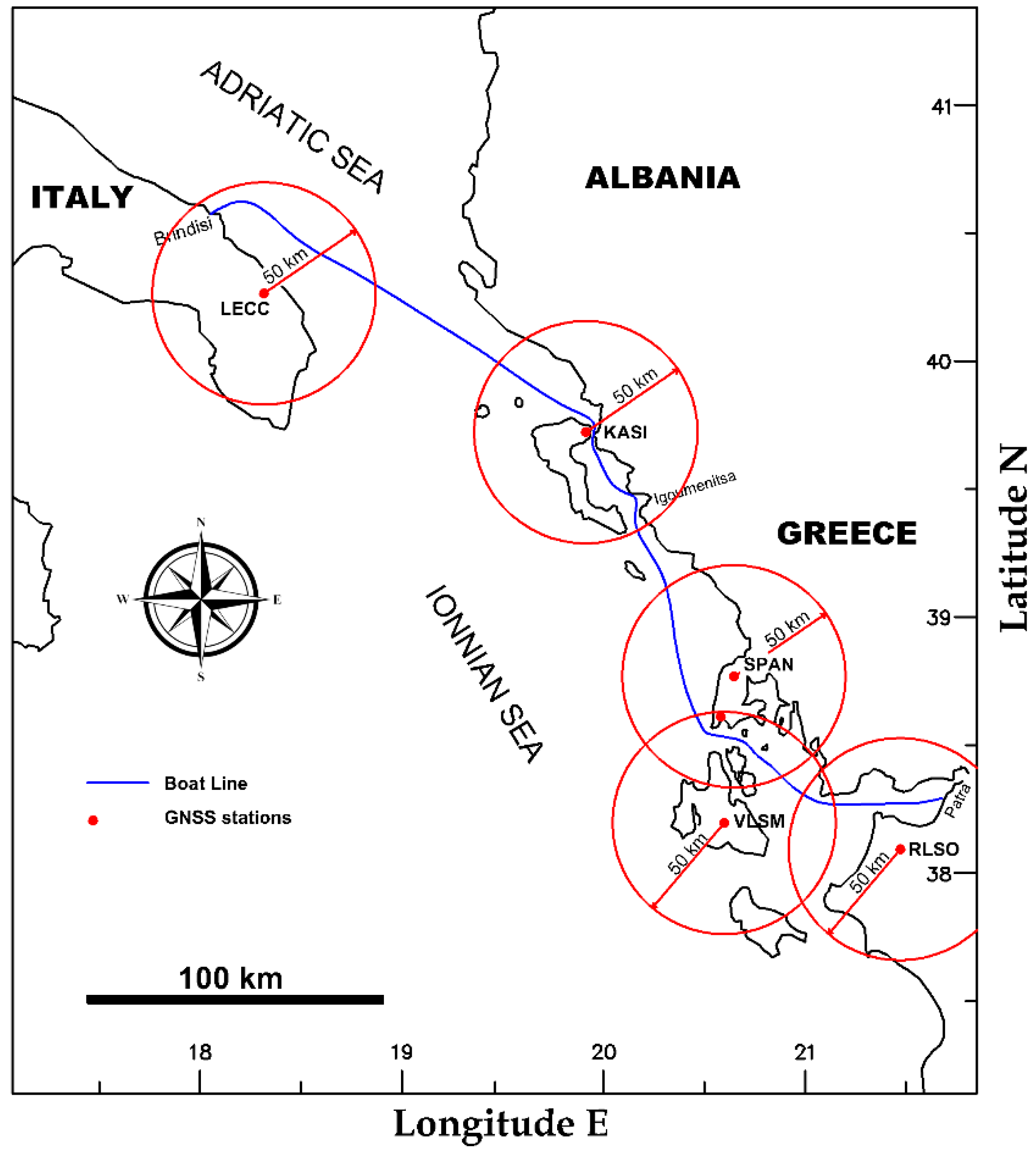
It is evident that the noise level is generally increased with the distance of the base station from the part of the ship’s journey in focus. In this study, we have generally adopted the critical distance of 50 km in order to ensure high reliability. However, this distance is rather specific, as resolving can be done successfully over somewhat larger distances. An overview of the parts of the route situated inside the distance of the 50 km from a given base station is illustrated in Figure 11. It is seen that the area south of Igoumenitsa and a large area between Corfu and Brindisi are located at distances greater than 50 km from base stations. In view of the above, we are accepting the individual solutions of a given base station, for a given part of the route on the basis of their proximity. For example, the individual solutions from the LECC station were used for the part of the route inside the upper–left circle of Figure 11. From the parts of the route being outside the radius of 50 km, we have used the closest neighboring base station from a given point of the route.

An example of the solution following this approach is illustrated in Figure 12.

It concerns the final configuration of a “combinatorial” solution using the segments that we consider as most appropriate for the path ID 71, taken as an example. It should be stressed that the synthesis of the solutions was not automated. It was done by examining the suitability of the individual solutions from each station with respect to the noise level. In this example (path ID 71), the solutions of the VLSM and SPAN stations were not used because in the parts c–e their signals had more noise than PONT. A comparison of the results illustrated in Figure 12 with those illustrated in Figure 10 and Figure S3 clearly shows that the above described approach leads to significant decrease of the noise level.

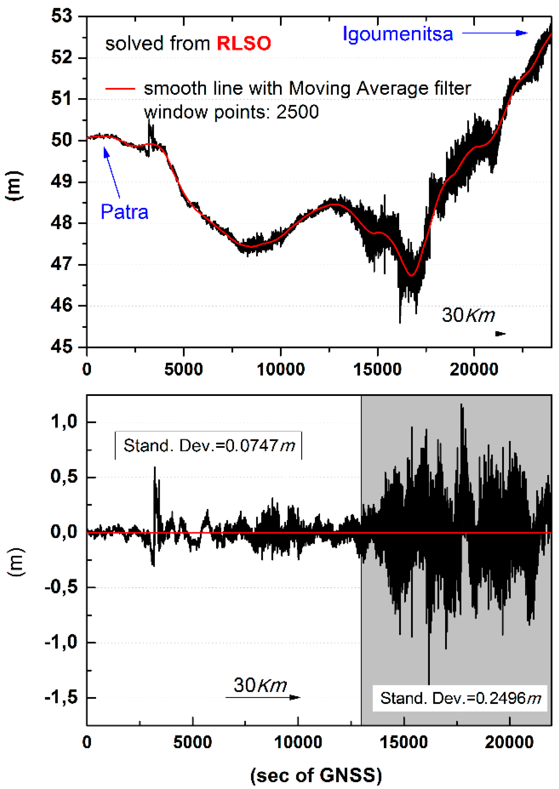
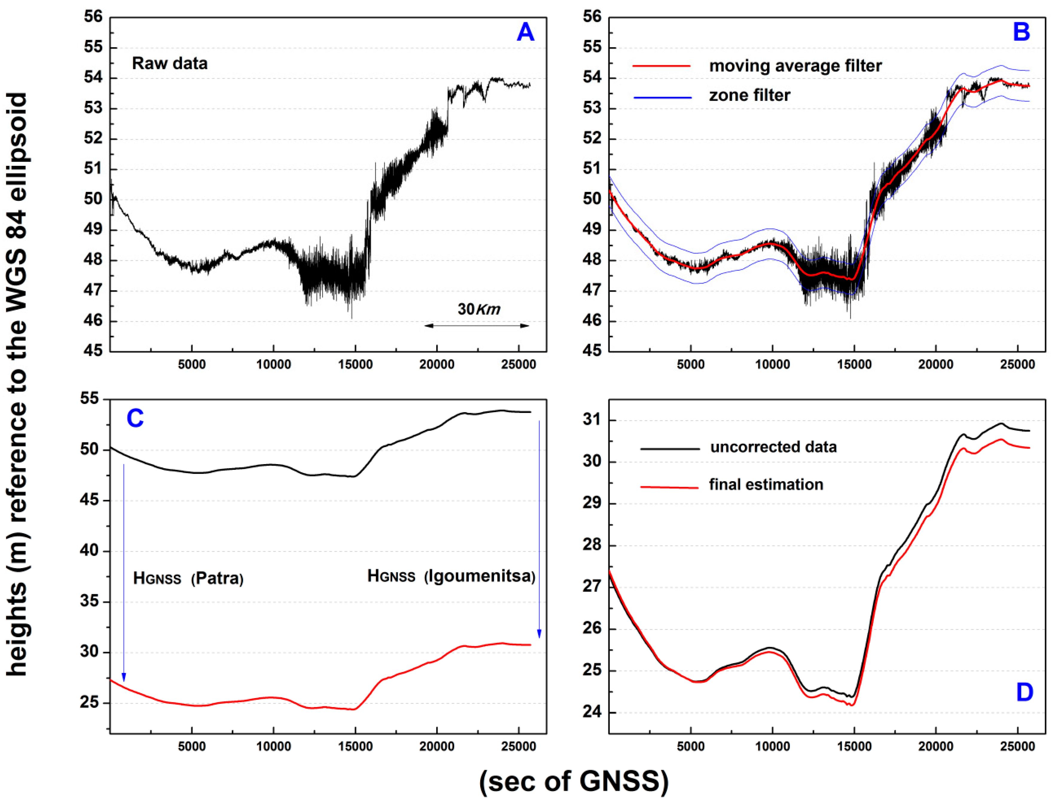
To decrease the noise level further, we proceeded to a noise correction with the Savitzky–Golay filter. The filter is based on the repeated adjustment of a polynomial utilizing the least squares method [39]. Figure 13 (top) illustrates the part of the Patra–Igoumenitsa route resolved by the RLSO station and the estimate of the moving average (red line). By subtracting the original signal from the estimates of the moving average, Figure 13 (bottom) was obtained. The left-hand side of the figure (white) represents part of the route near the settlement station, justifying the quite small standard deviation. In contrast, the differences on the right-hand side of the figure (gray), representing part of the route at a significant distance from the settlement station, are characterized by larger standard deviation. This was to be expected, taking into account the considerations of the previous paragraph.

The technique of the Savitzky–Golay moving average filter does not only correct the noise of GNSS measurements, but also the wave dynamic effect. As already mentioned, the wave action on a big ship is practically negligible because it is eliminated by the dynamic behavior of the ship’s construction; only waves higher than 4 m and longer than 10 m can exert a significant effect [8]. However, even in this case the action of the filter permanently eliminates this dynamic phenomenon.

3.5. Solution of the GNSS Raw Data for Determining the H(i,t) Values Following the PPP Method

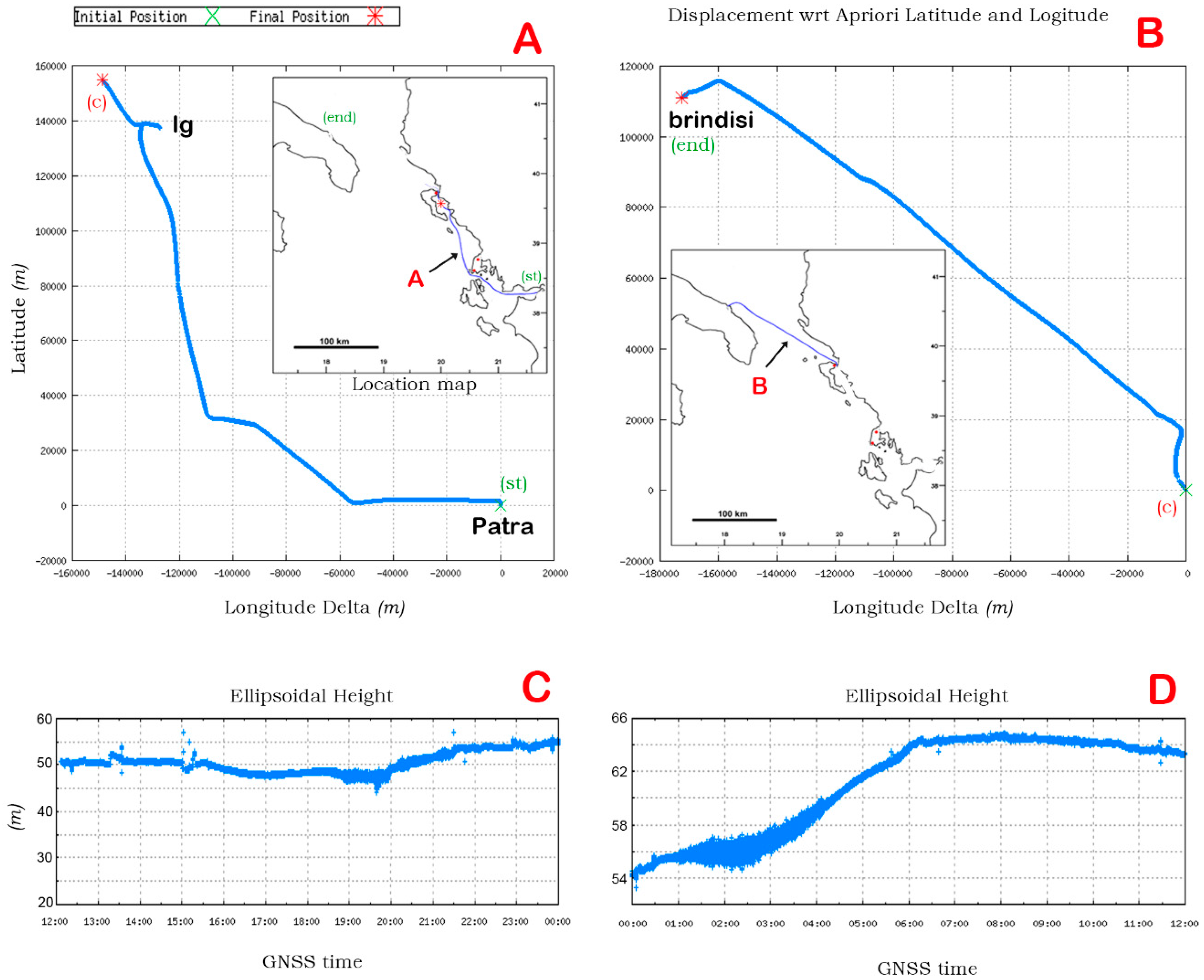
As an alternative to the D-GNSS method, all route data were also resolved by the PPP method. The PPP method does not need reference stations, and thus it is at an advantage regarding the sections of the route that are at long distances (<50 km) from these stations. As the track logs were large in volume and could not be resolved with the current features of the editor, they were split into shorter records. In this way the routes were divided in half and doubled in their number. In Figure 14 shows a solution with the PPP methodology. It concerns the two sections in which a given route has been divided.

The steps followed in the previously described D-GNSS analysis were also followed here except for base stations, as this is not necessary in the PPP method. These are illustrated in Figure 15. The figure concerns the “Patra–Igoumenitsa“ route with code ID1, taken as an example. Three other examples concerning the routes with codes ID3, ID11 and ID141 are illustrated in the Figures S3–S5.

In all cases, the curve in part A of each of the aforementioned figures describes the raw data. Three of the four examples concern the middle of winter (end of January, ID1, ID3 and ID11) with adverse weather conditions, while the fourth (ID141) concerns mid-summer with very smooth weather conditions (see Table S1). The examples were chosen to render visible the large difference in the range of noise we encounter when the weather changes. It is evident that the range of noise is much greater in the passes with code numbers ID1, ID3 and ID11 illustrated in Figure 15, Figures S3 and S4 than that in the route ID141 illustrated in Figure S5.

Part B of each of the aforementioned figures presents the curve with the original data; the curve of mean values (red curve) obtained by applying the Savitzky–Golay method [38]; and the two light-blue curves, which indicate a band filter selected to have a total width of 1 m beyond which each value was deducted. It can be seen that the band filter does not remove any value, as the range of all values is smaller than the bandwidth, in the last example (Figure S5B) referring to good weather conditions.

In part C, of each of the aforementioned figures, the h_GNSS receiver elevation correction at port check points described in Section 3.2 is illustrated. The height of the receiver on the vessel measured at the ports was removed from the data in order to generate the height of the sea topography.

Finally, in part D of the aforementioned figures, the linear correction concerning the influence of astronomical and meteorological components of tide, $h_{tide}$, which is based on calculations of altitude in ports described in Section 3.3, is illustrated. With this correction, as explained earlier, the effect of the tide was removed.

3.6. Outline of the Analysis Procedure

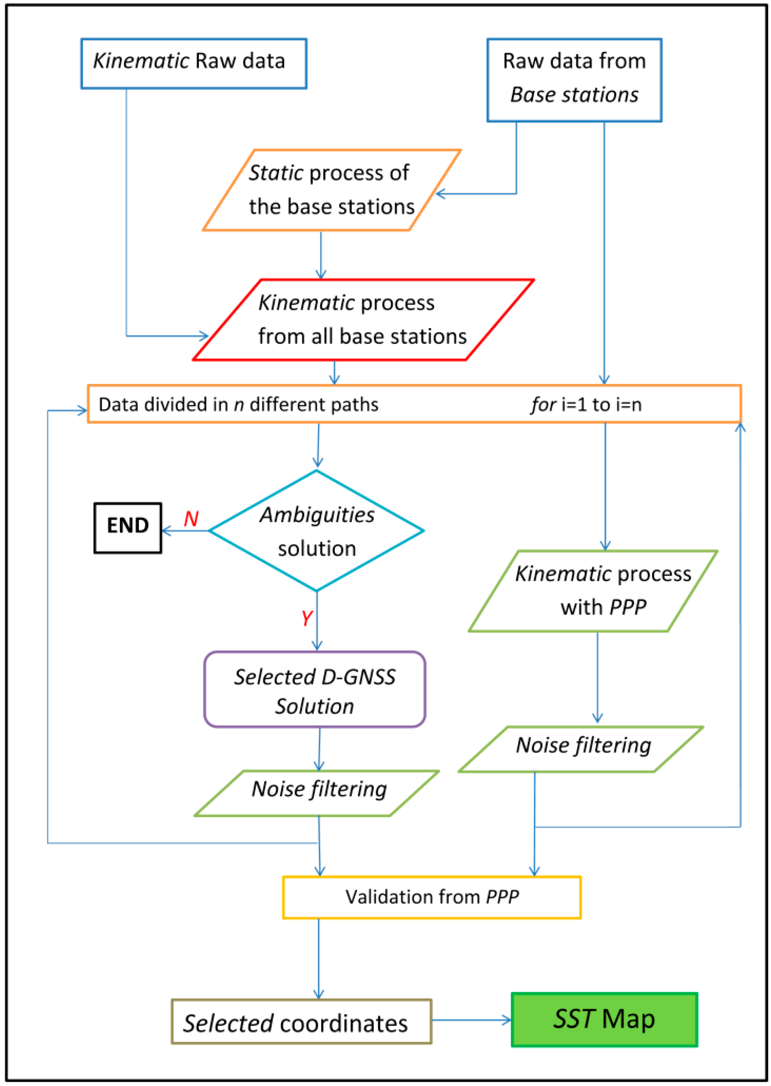
In this section, the analysis procedure that has been followed to render it more comprehensible is briefly visualized. The basic steps of the methodology are illustrated in Figure 16 in the form of a flowchart. The raw GNSS data are those obtained from ship’s routes (kinematic raw data) and those obtained from the ground stations. The first step involved static solutions in the base stations, whereas the second step was a kinematic solution of all routes from all base stations following the D-GNSS method. Then two different calculations were done in parallel. One concerned the application of the D-GNSS method, and the second, the application of the PPP method. Concerning the D-GNSS application, it was first examined whether the D-GNSS (LGO) software resolved the uncertainties relevant to a given route. If that had not happened, the results were discarded. For the routes where the uncertainties were resolved, a combinatorial solution was chosen (Section 3.4, Figure 10). After this selection, the procedure involved numerical filtering (Section 3.4, Figure 13), followed by the removal of static heights of the receiver (Section 3.2, Equation (3), Figure 7) and then the linear tidal correction described in Section 3.3.

A parallel process was followed with the PPP method. The only exception was that the procedure did not involve the aforementioned combinatorial solution, but a simple solution from the beginning. Once all the paths were resolved, the ones that had been solved were selected. Then the procedure involved noise removal by numerical filtering, the removal of static heights of the receiver (Section 3.2, Equation (3), Figure 7) and then the linear tidal correction described in Section 3.3 (see also Figure 15 and Figures S4–S6).

Having achieved the estimates of the Ψ(i) values from both methods, we proceeded to a final assessment of the marine topography by calculating the dynamic means both between the individual routes–resolutions and between the different methods. This allowed constructing the map of the mean marine topography for the area studied.

4. Estimation of the Mean Sea Level in the Area Studied

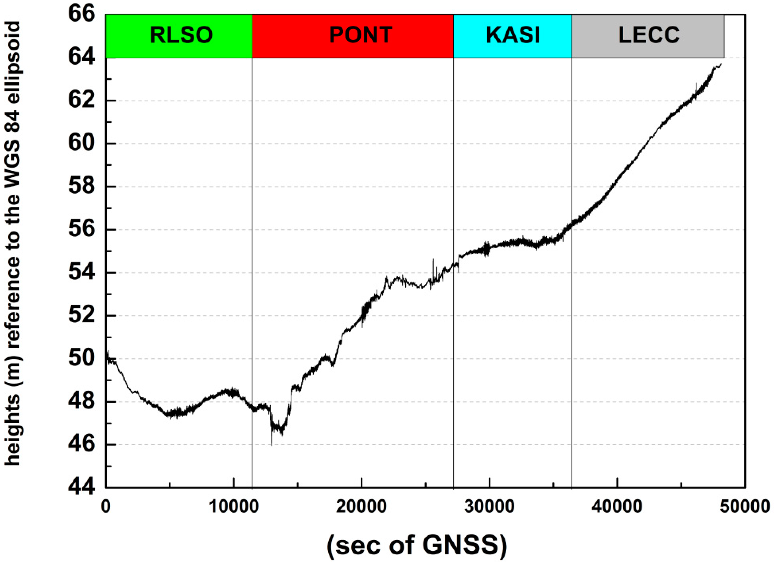
On the basis of what were described above, the final assessment of the mean marine topography in the studied area was achieved (Figure 17).

This assessment was obtained while taking into account jointly the final calculations performed using the D-GNSS and PPP methods. It is worth noting that for each Ψ(i) (line segment vertically intersecting all the different paths; see Figure 6), the average of all estimates from all the crossings for both methods was calculated. When creating the map illustrated in Figure 17, as an application area on the horizontal plane, we considered a zone that encompasses all the ship’s routes and covers an area of tens of meters up to a few kilometers on either side of the principal route. It is evident that we can distinguish very significant altitude differences of up to 16 m. Moreover, the marine topography in the region shows a nearly constant slope of 4 cm/km in the N–S direction.

A final estimation of the accuracy of the contour map (parameter u(i,t) in Equation (1)) was obtained while taking into account the following: (a) the accuracy of calculating the height of the h_GNSS receiver based on the draught measurements (Section 3.2), (b) the mean range of the standard deviation of the differences of the kinematic data from the mean value, as it was derived by the moving average filter (e.g., Figure 13, Figure 15B, Figures S4B, S5B and S6B) and (c) the standard deviation of static estimations at ports (Figure 8). Factors α and β were thought to contribute linearly to the final estimate of uncertainty. Concerning factor c, the linear correction described in the Section 3.3 eliminates completely the factors of the meteorological component. However, it would be rather exaggerated to consider complete elimination of this parameter, as we cannot assess the tidal effect upon travel, except in the ports. Thus, adopting a more rigorous approach, we assumed an uncertainty of 2 cm as a representative value of the tide in this area. By taking into account the influence of factors a, b and c and using the well-known error transmission law, an accuracy of 3.31 cm was obtained for the MSL in the area studied (σ_hMSL = 3.31 cm).

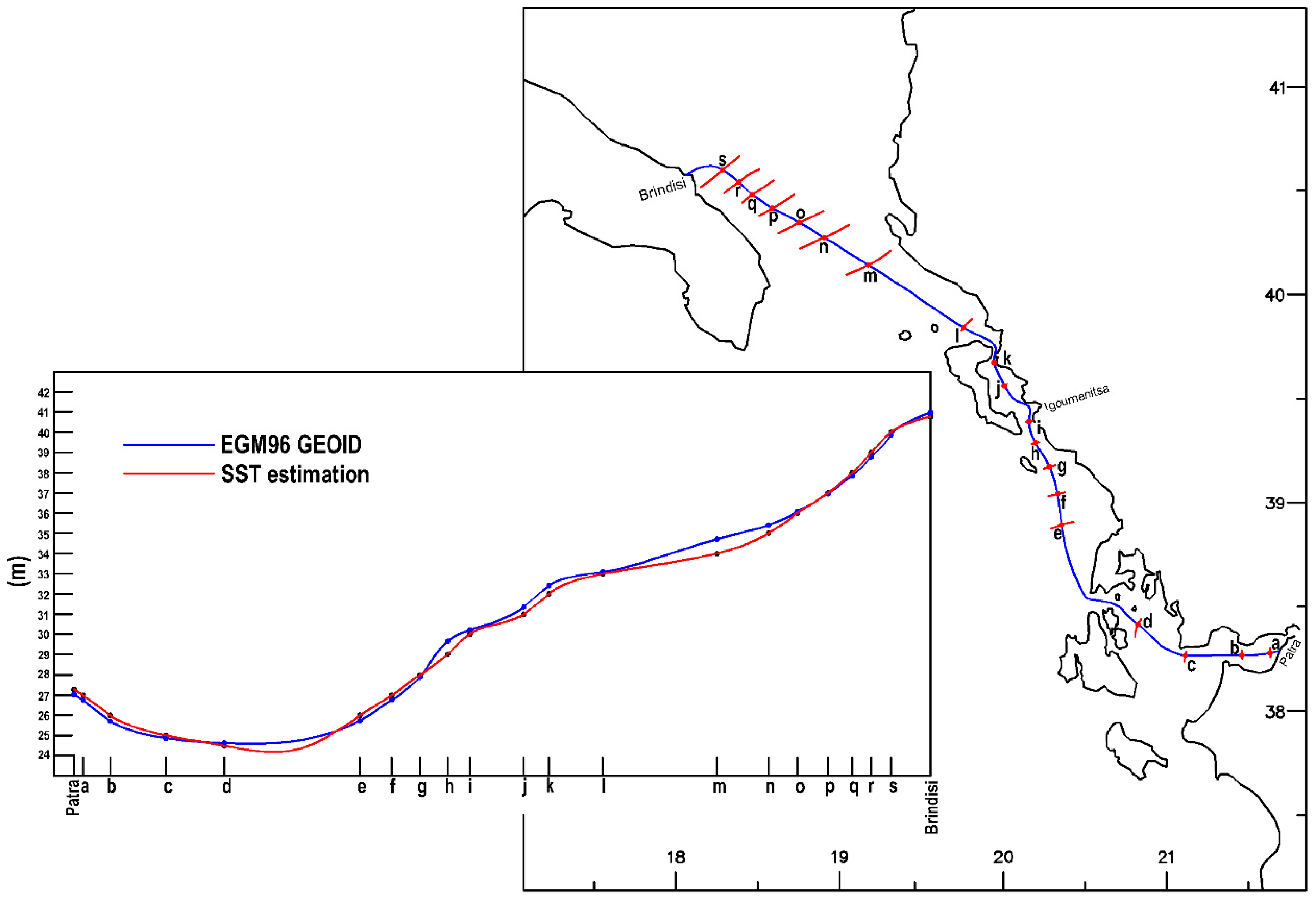
Finally, the results of the proposed methodology are compared to those of the geoid model EGM96 (Figure 18). Taking into account the accuracy of the EGM96′s own estimates and other estimates of the mean sea level, the differences are relatively small (up to 50 cm). The most significant difference is between points I and O, north of Corfu, where our estimate appears to be significantly lower than the estimates of EGM96, up to a maximum of 48 cm.

5. Concluding Remarks

• The precision was estimated as 3.31 cm, taking into account all the uncertainty factors under quite rigorous assumptions. Higher precision would be achieved by further use of the proposed methodology.
• The precision of the factor h_GNSS based on the measurements, is actually much higher (σ: 0.76 cm). Nevertheless, due to factors that could not be accurately determined (e.g., due to the lack of tide data in the area), we adopted a much more conservative approach, increasing the σ value to 3.1 cm. Nonetheless, the precision determined by the measurements is the highest ever published. This indicates the great potential for improvement of the method “repeated GNSS measurements on the same route of a ship”, in the near future.
• The significant differences between the estimates of the present work (SST estimate) and the geoid model (EGM96) in the d, e and m regions may be related to strong tectonic changes of the marine subsoil. In fact, in both areas strong tectonic activity has been inferred [39,40]. Moreover, recent studies have provided evidence for serious deposits in the area [41]. However, further investigation is required to corroborate this evidence.
• The application of this approach using systematic multi-track recordings on conventional liner ships is very promising, as it may open up possibilities for widespread use of the methodology across the world.
• Τhe focus of floating GNSS on specific areas in conjunction with satellite data can provide complex, localized, high-precision solutions. The “GNSS method on floating means” can cover the areas not covered by the scanning of altitude satellites and thus may provide an important service in the exploration of marine topography.

References

- Pascual, A.; Pujol, M.I.; Larnicol, G.; Le Traon, P.Y.; Rio, M.H. Mesoscale mapping capabilities of multisatellite altimeter missions: First results with real data in the Mediterranean Sea. J. Mar. Syst. 2007, 65, 190–211. [Google Scholar] [CrossRef]
- Cocard, M.; Geiger, A.; Kahle, H.G.; Veis, G. Airborne laser altimetry in the Ionian Sea, Greece. Glob. Planet. Chang. 2002, 34, 87–96. [Google Scholar] [CrossRef]
- Lycourghiotis, S.; Stiros, S. Sea Surface Topography in the Gulf of Patras and the southern Ionia sea using GPS. In Proceedings of the 12th Internasional Congress of the Geological Society of Greece, Patras, Greece, May 2017; Volume XLIII, pp. 1029–1034. [Google Scholar]
- Bonnefond, P.; Exertier, P.; Laurain, O.; M’enard, Y.; Orsoni, A.; Jan, G.; Jeansou, E. Absolute Calibration of Jason-1 and TOPEX/Poseidon Altimeters in Corsica. Mar. Geod. 2003, 26, 261–284. [Google Scholar] [CrossRef]
- Rocken, C.; Johnson, J.; Van Hove, T.; Iwabuchi, T. Atmospheric water vapor and geoid measurements in the open ocean with GPS. Geophys. Res. Lett. 2015, 32. [Google Scholar] [CrossRef] [Green Version]
- Foster, H.; Carter, G.S.; Merrifield, M.A. Ship-based measurements of sea surface topography. Geophys. Res. Lett. 2009, 36. [Google Scholar] [CrossRef]
- Bouin, M.-N.; Ballu, V.; Calmant, S.; Boré, J.-M.; Folcher, E.; Ammann, J. A kinematic GNSS methodology for sea surface mapping, Vanuatu. J. Geod. 2009, 83, 1203–1217. [Google Scholar] [CrossRef]
- Reinking, J.; Härting, A.; Bastos, L. Determination of sea surface height from moving ships with dynamic corrections. J. Geod. Sci. 2012. [Google Scholar] [CrossRef]
- Guo, J.; Liu, X.; Chen, Y.; Wang, J.; Li, C. Local normal height connection across sea with ship-borne gravimetry and GNSS techniques. Mar. Geophys. Res. 2014, 35, 141–148. [Google Scholar] [CrossRef]
- Chupin, C.; Ballu, V.; Testut, L.; Tranchant, Y.T.; Calzas, M.; Poirier, E.; Bonnefond, P. Mapping Sea Surface Height Using New Concepts of Kinematic GNSS Instruments. Remote Sens. 2020, 12, 2656. [Google Scholar] [CrossRef]
- Lycourghiotis, S. Developing a GNSS-on-boat based technique to determine the shape of the sea surface. In Proceedings of the 7th International Conference on Experiments/Process/System Modeling/Simulation/Optimization, Athens, Greece, 5–8 July 2017; Volume I, pp. 113–119, ISSN: 2241-9209, ISBN SET: 978-618-82173-2-4, ISBN Vol. I: 978-618-82173-3-1. [Google Scholar]
- Lycourghiotis, S. Sea surface topography determination. Comparing two alternative methods at the Gulf of Corinth. In Proceedings of the 7th International Conference on Experiments/Process/System Modeling/Simulation/Optimization, Athens, Greece, 5–8 July 2017; Volume II, pp. 410–415, ISSN: 2241-9209, ISBN SET: 978-618-82173-2-4, ISBN Vol. II: 978-618-82173-4-8. [Google Scholar]
- Lycourghiotis, S. Improvements of GNSS–on-boat methodology using a catamaran platform: Application at the gulf of Patras. In Proceedings of the 7th International Conference on Experiments/Process/System Modeling/Simulation/Optimization, Athens, Greece, 5–8 July 2017; Volume I, pp. 255–261, ISSN: 2241-9209, ISBN SET: 978-618-82173-2-4, ISBN Vol. I: 978-618-82173-3-1. [Google Scholar]
- Bonnefond, P.; Exertier, P.; Laurain, O.; Thibaut, P.; Mercier, F. GPS-based sea level measurements to help the characterization of land contamination in coastal areas. Adv. Space Res. 2013, 51, 1383–1399. [Google Scholar] [CrossRef]
- Kelecy, T.M.; Born, G.H.; Parke, M.E.; Rocken, C. Precise mean sea level measurements using the Global Positioning System. J. Geophys. Res. Ocean. 1994, 99, 7951–7959. [Google Scholar] [CrossRef]
- Marshall, A.; Denys, P. Water level measurement and tidal datum transfer using high rate GPS buoys. N. Z. Surv. 2009, 299, 24. [Google Scholar]
- Key, K.W.; Parke, M.E.; Born, G.H. Mapping the sea surface using a GPS buoy. Mar. Geod. 1998, 21, 67–79. [Google Scholar] [CrossRef]
- Kato, T.; Terada, Y.; Kinoshita, M.; Kakimoto, H.; Isshiki, H.; Moriguchi, T.; Johnson, J. A new tsunami monitoring system using RTK-GPS. In Proceedings of the International Tsunami Symposium, Seattle, WA, USA, 7–10 August 2001; pp. 5–12. [Google Scholar]
- Doong, D.J.; Lee, B.C.; Kao, C.C. Wave measurements using GPS velocity signals. Sensors 2011, 11, 1043–1058. [Google Scholar] [CrossRef]
- Wöppelmann, G.; Miguez, B.M.; Bouin, M.N.; Altamimi, Z. Geocentric sea-level trend estimates from GPS analyses at relevant tide gauges world-wide. Glob. Planet. Chang. 2007, 57, 396–406. [Google Scholar] [CrossRef] [Green Version]
- Deng, X.; Featherstone, W.E.; Hwang, C.W.; Berry, P.A.M. Estimation of contamination of ERS-2 and POSEIDON satellite radar altimetry close to the coasts of Australia. Mar. Geod. 2002, 25, 249–271. [Google Scholar] [CrossRef]
- Hipkin, R. Modelling the geoid and sea-surface topography in coastal areas. Phys. Chem. Earth Part A Solid Earth Geod. 2000, 25, 9–16. [Google Scholar] [CrossRef]
- Majumdar, T.J. Satellite Geoid/Gravity for Offshore Exploration. In Geospatial Technologies and Climate Change; Springer: Cham, Switzerland, 2014; pp. 203–218. [Google Scholar]
- Karakitsios, V. Western Greece and Ionian Sea petroleum systems. AAPG Bull. 2013, 97, 1567–1595. [Google Scholar] [CrossRef] [Green Version]
- Lemoine, F.G.; Kenyon, S.C.; Factor, J.K.; Trimmer, R.G.; Pavlis, N.K.; Chinn, D.S.; Wang, Y.M. The development of the joint NASA GSFC and the National Imagery and Mapping Agency (NIMA) geopotential model EGM96. In Gravity, Geoid and Marine Geodesy; Springer: Berlin/Heidelberg, Germany, 1998. [Google Scholar]
- Vignudelli, S.; Cipollini, P.; Roblou, L.; Lyard, F.; Gasparini, G.P.; Manzella, G.; Astraldi, M. Improved satellite altimetry in coastal systems: Case study of the Corsica Channel (Mediterranean Sea). Geophys. Res. Lett. 2005, 32, L07608. [Google Scholar] [CrossRef]
- Jin, S.; Cardellach, E.; Xie, F. GNSS Remote Sensing; Springer: Dordrecht, The Netherlands, 2014. [Google Scholar]
- GGrejner-Brzezinska, D.A.; Kashani, I.; Wielgosz, P. On accuracy and reliability of instantaneous network RTK as a function of network geometry, station separation, and data processing strategy. GPS Solut. 2005, 9, 212–225. [Google Scholar] [CrossRef]
- Malinowski, M.; Kwiecień, J. A comparative study of Precise Point Positioning (PPP) accuracy using online services. Rep. Geod. Geoinformatics 2016, 102, 15–31. [Google Scholar] [CrossRef] [Green Version]
- Larsson, P.; Henriksson-Larsén, K. The use of dGPS and simultaneous metabolic measurements during orienteering. Med. Sci. Sports Exerc. 2011, 33, 1919–1924. [Google Scholar] [CrossRef]
- Zumberge, J.F.; Heflin, M.B.; Jefferson, D.C.; Watkins, M.M.; Webb, F.H. Precise point positioning for the efficient and robust analysis of GPS data from large networks. J. Geophys. Res. 1997, 102, 5005–5017. [Google Scholar] [CrossRef] [Green Version]
- Tsimplis, M.N.; Proctor, R.; Flather, R.A. A two-dimensional tidal model for the Mediterranean Sea. J. Geophys. Res. Ocean. 1995, 100, 16223–16239. [Google Scholar] [CrossRef]
- Cheng, Y.; Andersen, O.B. Improvement in global ocean tide model in shallow water regions. In Proceedings of the OSTST2010, Lisbon, Portugal, 18–20 October 2010. [Google Scholar]
- Lozano, C.J.; Candela, J. The M (2) tide in the Mediterranean Sea: Dynamic analysis and data assimilation. Oceanologicaacta 1995, 18, 419–441. [Google Scholar]
- Lycourghiotis, S.; Kontoni, D.-P.N. Analysing the Flood Risk in Mediterranean Coastal Areas with a New Methodology. In Proceedings of the 5th International Conference from Scientific Computing to Computational Engineering, Athens, Greece, 4–7 July 2012; Volume I, pp. 74–79, ISBN SET: 978-960-98941-9-7, ISBN Vol. I: 978-618-80115-0-2. [Google Scholar]
- Lycourghiotis, S.A.; Stiros, S.C. Coastal Flooding Hazard in Low-Tide and High-Tide Coasts: Evidence from the North Aegean Coast. In Coastal Hazards; Springer: Dordrecht, The Netherlands, 2013; pp. 231–243. [Google Scholar]
- Lycourghiotis, S.; Stiros, S. Meteorological tide and food risk at the Aegean basin. In Proceedings of the 4th Congress, Management and Improvement of Coastal Zones, Lesvos, Greece, 23–27 September 2008; pp. 63–73. [Google Scholar]
- Grejner-Brzezinska, D.A.; Wielgosz, P.; Kashani, I.; Smith, D.A.; Spencer, P.S.; Robertson, D.S.; Mader, G.L. An analysis of the effects of different network-based ionosphere stimation models on rover positioning accuracy. Positioning 2004, 1, 115–131. [Google Scholar] [CrossRef] [Green Version]
- Louvari, E.; Kiratzi, A.A.; Papazachos, B.C. The Cephalonia transform fault and its extension to western Lefkada Island (Greece). Tectonophys. 1999, 308, 223–236. [Google Scholar] [CrossRef]
- Altıner, Y.; Bačić, Ž.; Bašić, T.; Coticchia, A.; Medved, M.; Mulić, M.; Pavlides, S. Present-day tectonics in and around the Adria plate inferred from GPS measurements. Postcollisional tectonics and magmatism in the Mediterranean region and Asia. Spec. Pap. Geol. Soc. Am. 2006, 409, 43–55. [Google Scholar]
- Zelilidis, A.; Maravelis, A.G.; Tserolas, P.; Konstantopoulos, P.A. An overview of the petroleum systems in the Ionian Zone, onshore NW Greece and Albania. J. Pet. Geol. 2015, 38, 331–348. [Google Scholar] [CrossRef]
Figure 1.
Trajectories of the TOPEX/POSEIDON, Jason-1, Jason-2, Envisat and ERS-2 satellites in the eastern Mediterranean region. The dark area describes our study area.
Figure 2.
The “Ionian Queen” passenger ship used for the Ionian and Adriatic Sea measurements, and the basic Global Navigation Satellite System (GNSS) equipment. The antenna of the receiver was placed at point A with a tribrach in order to ensure leveling. The receiver was placed at point B in a special waterproof case for its protection.
Figure 3.
Schematic representation of the ship “Ionian Queen.” The points of calculation concerning the elevation (draught) of the ship up on its loading are illustrated. The projection of the position of the receiver on the AB segment divides it into two subsections, ΧΑ and ΧΒ.
Figure 4.
Map of the study area showing the ship’s principal route as well as the GNSS ground stations used during the processing. The route was not exactly the same each time, because the ship followed a slightly different path on each voyage. The points a–s marked here along the “principal route” refer to some of the figures. The stations RLSO, VLSM, PONT, SPAN and KASI belong to the National Observatory of Athens (NOANET GNSS NETWORK), and the station LECC to the Italian Positional Service (ItalPoS).
Figure 5.
Parameters of Equation (1). The red line depicts the mean seal level (MSL), and the light blue line illustrates the sea level at a given time without the wave effect.
Figure 6.
Different routes near to the port of Brindisi which are indicated by different colors. The routes were taken place in the period 3–11/2/2010 corresponding to ID numbers 5–13 (Table S1). The dots i, i + 1, i + 2, i + 3, i + 4, etc., represent indicative measurements on route 1.
Figure 7.
Geometric calculation of the antenna height with respect to the plane of the sea surface. The calculation is based on the draught at points A and B, which must be measured at each port before the ship leaves and after the final loading (moving loads, tanks). The data of the draught at points A and B were calculated by an electronic sensor and recorded in the ship’s book.
Figure 8.
Graphic representations of the elevation values in the ports of Patras and Brindisi. The average altitudes in the two ports (mean values) and the standard deviation values are illustrated.
Figure 9.
Horizontal coordinates of the ship’s principal path as solved by the PONT-based D-GNSS method. The logs refer to the route from Patras to Brindisi with a stop at Igoumenitsaat 30/31-1-2010 (Route ID 1). Coordinates are in UTM meters (UTM zone 34N).
Figure 10.
Typical examples of initial D-GNSS solutions by: VLSM (ID route 18), RLSO (ID route 24), SPAN (ID route 110) and LECC (Stack ID route 2). The points a–s are the route points illustrated in Figure 4. Thus, they visualize the parts of the route presented each time. Indicative lengths inside the parts of the route presented each time are illustrated. The values illustrated on the y-axis have not been corrected for the height of the receiver relative to the sea surface, hGNSS.
Figure 11.
An overview of the parts of the route situated inside of the distance of the 50 km from a given base station. The base station PONT (Figure 4) is not presented here for clarity reasons because the corresponding circle is strongly overlapped with the circles of base stations VLSM and SPAN.
Figure 12.
Example of a “combinatorial” solution using the D-GNSS method for path ID 71. The RLSO, PONT, KASI and LECC stations have been used. The RLSO, PONT, KASI and LECC stations were used, respectively, for the parts of the route, Patras to c, c to g, g to m and m to Brindisi. The values illustrated on the y-axis have not been corrected for the height of the receiver relative to the sea surface, hGNSS.
Figure 13.
(top): An example of solving the sea altitude of the route (Patras–Igoumenitsa) (points a to k; see Figure 4) which was resolved by the RLSO station using the D-GNSS method (ID route 3). This displays different noise levels in relation to the distance of the measuring station. The red line represents the adjusted moving average curve. Indicative length is illustrated. The values illustrated on the y-axis have not been corrected for the height of the receiver relative to the sea surface, hGNSS. (Bottom): Differences (residues) from the moving average curve. The standard deviation in the first segment is much smaller than that in the second segment, which represents part of the route at a great distance from the base station. Indicative length is illustrated.
Figure 14.
Solving with the PPP method on a horizontal and a vertical plane. (A,B) Resolved horizontal coordinates, track ID. (A) The route between Patras and Igoumenitsa (30 January). (B) The rest of the route up to the port of Brindisi (31 January). (C,D) The vertical components of the sections (A,B), respectively.
Figure 15.
Illustration of the Patra–Igoumenitsa route with ID1 (see Table S1). (A) The raw data of the GNSS altitude during the route as they emerged from the PPP solution. (B) The raw data, the curve of mean values (red curve) obtained by applying the Savitzky–Golay moving average filter and the two curves (light blue) indicating the limiting values imposed by the band filter. (C) hGNSS receiver elevation correction at port check points described in Section 3.2. (D) Linear correction based on deviations of measured port levels from the medium marine level (linear tidal correction described in Section 3.3). (For more examples see also: Figure S3–S5).
Figure 16.
Illustration of the basic methodology developed in the present work.
Figure 17.
Sea surface topography in the area studied. The heights were calculated while taking as reference the ellipsoid WGS 84. The numbers illustrated concern the corresponding segments.
Figure 18.
Comparison of the final results (principal route) of this work with the geoid model EGM96. We observe general agreement of our results with those of the geoid and small variations (<50 cm). The heights were calculated based on the reference ellipsoid WGS 84.
Publisher’s Note: MDPI stays neutral with regard to jurisdictional claims in published maps and institutional affiliations. |
© 2021 by the author. Licensee MDPI, Basel, Switzerland. This article is an open access article distributed under the terms and conditions of the Creative Commons Attribution (CC BY) license (http://creativecommons.org/licenses/by/4.0/).
Share and Cite
MDPI and ACS Style
Lycourghiotis, S. Sea Topography of the Ionian and Adriatic Seas Using Repeated GNSS Measurements. Water 2021, 13, 812. https://doi.org/10.3390/w13060812
AMA Style
Lycourghiotis S. Sea Topography of the Ionian and Adriatic Seas Using Repeated GNSS Measurements. Water. 2021; 13(6):812. https://doi.org/10.3390/w13060812
Chicago/Turabian StyleLycourghiotis, Sotiris. 2021. "Sea Topography of the Ionian and Adriatic Seas Using Repeated GNSS Measurements" Water 13, no. 6: 812. https://doi.org/10.3390/w13060812
Note that from the first issue of 2016, this journal uses article numbers instead of page numbers. See further details here.