
Water–Food–Energy Nexus Tradeoffs in the São Marcos River Basin
by
 ,
,
Pedro Henrique Bof
1,* ,
,
Guilherme Fernandes Marques
1,
Amaury Tilmant
2,
Ana Paula Dalcin
1 and
Marcelo Olivares
3,4 1
Institute of Hydraulic Research (IPH), Universidade Federal do Rio Grande do Sul (UFRGS), Porto Alegre-RS 90640-002, Brazil
2
Department of Civil and Water Engineering, Université Laval, Quebec City, QC G1V 0A6, Canada
3
Department of Civil Engineering, Universidad de Chile, Santiago 8330015, Chile
4
Energy Center, Universidad de Chile, Santiago 8320000, Chile
*
Author to whom correspondence should be addressed.
Water 2021, 13(6), 817; https://doi.org/10.3390/w13060817
Submission received: 8 December 2020
/
Revised: 5 February 2021
/
Accepted: 10 March 2021
/
Published: 16 March 2021
(This article belongs to the Special Issue Water Management for Agricultural, Environmental and Urban Uses)
Abstract
:Given its potentialities and characteristics, energy generation, food production, and water availability have a strong interdependency and correlation. Water is needed to produce energy and food, while energy is required to produce water and food. This nexus brings several challenges when scarce water resources must be allocated among competing uses, often in the form of unexpected tradeoffs. Addressing those challenges requires knowledge about the water–food–energy nexus and the associated tradeoffs to support water allocation and management decisions. Those tradeoffs are still not properly understood in the uncertain and stochastic context of water availability. When not properly accounted for, the results are conflicts, loss of investments, environmental impacts, and limited effectiveness of sectoral policies, all of which undermine a country’s development model relying on water and energy security. This paper addresses the competitive uses of recent irrigated agriculture expansion and existing hydropower production in a Brazilian watershed with water conflicts, assessing the economic tradeoffs and water values between energy and irrigated agricultural production under uncertainty. An explicitly stochastic hydro-economic model is used to determine water’s economic value and its variation in space and time. Results indicate that the agricultural benefits outweigh the potential energy losses, and the best course of action should explore an economically compensated reallocation strategy, upon negotiation among users, rather than imposing water supply cutbacks to the agriculture sector.
1. Introduction
As water systems evolve, accommodating new growing uses with existing ones becomes a challenge, potentially unfolding to conflicts, especially when systems were originally designed under predominant water use. In Brazil, recent conflicts between water users from different sectors have been registered in [1] with hydropower generation and industrial consumption; in [2] with irrigation, hydropower projects, and other social demands in the São Francisco River Basin; in [3] with hydropower and urban water supply sectors in the Billings and Barra Bonita multiple-use reservoirs; in [4] with irrigators in Campos dos Goytacazes, Rio de Janeiro, Brazil; in [5] with local government, society and business people in the São Luiz do Tapajós hydropower plant and in [6] between two states that share the waters of the basin in the Piranhas-Açu River Basin.
These examples highlight an increasingly common problem shared by many regions globally, with water systems struggling to adapt to new conditions [7,8]. New water uses often broaden the scope of the issues, especially when there is a strong nexus between water, food production, and energy [9]. Where a nexus exists, tradeoffs from water uses emerge [10], meaning that the use of water in one sector impacts the use in another sector. Food production demands water for irrigation which reduces firm energy yields for hydropower and flows for thermal plants cooling downstream while securing flows for long-term hydropower projects, restricting future irrigated agriculture expansion upstream of the power projects [11].
While higher and more diverse water uses to bring in more disputes and rivalry for water, it also means more development and economic diversification opportunities, strengthening the regional economy. In this context, water managers and users should strive to find solutions to accommodate new water uses towards regional economic development while avoiding conflict and environmental impacts from the nexus between energy, food (in the form of irrigated agricultural production), and water.
In this paper, we argue that an important step in solving these disputes is to identify and quantify the water–food–energy tradeoffs to fully understand the negotiation space and provide useful information to support water allocation and management [12].
Several studies point out the importance of the nexus between water, energy, and food production [8,9,10,13,14,15,16,17,18,19,20,21,22]. Water abstraction, pumping, and irrigation for crops require large amounts of energy for its implementation [20]. Currently, 70% of global water consumption is turned to agriculture [23], while the sector consumes 30% of the production chain’s global energy supply [24]. Simultaneously, 90% of the energy generated globally requires water in its generation. The energy sector was responsible for a water demand of 583 billion cubic meters in 2010, representing 15% of global water demand [25]. Daher and Mohtar [26] highlight the importance of the nexus and offer a framework and set of methodologies to define its links. As pointed out in [27], water scarcity challenges highlight the concept of nexus thinking, shifting from a sectoral focus on production maximization to improve efficiency across different involved sectors.
While the importance of the nexus is recognized, it is still poorly documented in a format to support conflict resolution and decision-making about water allocation. The latter demands an evaluation of tradeoffs between the nexus’ components and the water’s economic value, critical to negotiate water allocation among users and implement policies such as water pricing, an often difficult task in Brazil [28] and worldwide [29,30]. As water is allocated with limited knowledge about these tradeoffs, it addresses only the short-term and immediate uses, failing to recognize the consequences to other present and future ones.
The negotiation process to allocate and manage scarce water when in the conflict has already been initiated and become severely hampered and potentially biased, as the tradeoffs created by the water–energy–food nexus make it difficult to predict the impact of the solution adopted in the various elements of the nexus. On the other hand, in situations where the conflict has not yet developed, it is impossible to verify whether current sectoral decisions or policies are putting one element of the nexus in a collision course with another, which prevents water management resources from being truly integrated.
The use of modeling and systems analysis tools for water resources management, including optimization methods as the link between economics and engineering, has allowed managers to fully explore economic principles to aid decision-making in search of integrated and flexible solutions. Several works in the literature have explored this approach. In [31], a continental scale Hydro-economic model integrates biophysical, technological, and economic features to evaluate water–energy–land nexus, including the cost of water management options. However, the core optimization model is deterministic, with perfect foresight, and the tradeoffs are not explicitly evaluated. In [32], the synergies in the water–food–energy nexus are explored with an integrated hydro-economic optimization model. The authors quantified the tradeoffs between hydropower, irrigation, and fisheries under different operation and hydrological conditions, with a scenario-based approach, which is limited in capturing the broad spectrum of hydrological uncertainty. Finally, a review of the hydro-economic modeling for water-policy assessment [33] highlights that while most hydro-economic models assume perfect foresight, water managers cannot perfectly predict water availability and must deal with risks in decision-making. Along with other studies [29,34,35,36,37,38,39,40,41,42,43,44,45,46], the literature still present gaps in the study of tradeoffs in the water–energy–food nexus, especially in representing hydrological uncertainties and variability. Rising [47] have compared integrated assessment models (IAMs) with water–energy–food (WEF) models, showing that IAM provides cost–benefit economic valuation, in opposition to WEF, which takes into consideration hydrological risks while IAMs do not. However, the author argues that neither model has consistently engaged with the issue of optimization under uncertainty. Pereira-Cardenal et al. [48] applied an explicit stochastic approach to optimize water-power systems jointly and found out that water allocation between high productivity irrigation and hydropower could be improved. However, the tradeoffs were not explicitly evaluated, and the authors assumed constant willingness-to-pay for water, which could result in over or underestimation of irrigated agriculture benefits.
Considering the presented knowledge gaps, this paper brings in a contribution to the evaluation of water–energy–food nexus tradeoffs with a combination of (a) dynamic accounting of water flows and marginal water use values (varying in space and time) and (b) reliability analysis through a state-of-the-art explicit stochastic optimization model to account for hydrologic uncertainties. This addresses previous limitations as the deterministic, perfect foresight in [31], the scenario-based approach in [32], the decision-making risks in [33], and the constant willingness-to-pay for water in [48].
The methods and results presented here contribute to the water management field by providing specific tools and information on assessing economic tradeoffs between two users in a basin with conflict over water use related to occurrence probabilities. It should be useful to (a) identify the reflexes of allocation decisions in other elements of the nexus; (b) create conditions for integrated water resources management and their compatibility with other sectoral policies (for example, irrigated agriculture and expansion of energy generation), (c) create conditions for economic compensation instruments, which facilitate the acceptance of a given solution and reduce the possibility of time-consuming conflict, and (d) relate tradeoff economic information with the probability of occurrence related to hydrological uncertainty. We chose the São Marcos River Basin, in Brazil, as the study area, given existing conflicts between hydropower and irrigated agriculture. We aim to answer three main questions: (a) How much benefit could the energy sector potentially lose when water is shared economically with the agriculture sector? (b) How much benefit the agricultural sector brings into the system when water is shared with the energy sector? We also ask, (c) How likely are those benefit changes, considering hydrologic variability?
The following sections presents (1) an overview of the study area context and problems (the São Marcos River Basin), the main water uses (irrigated agriculture, hydropower generation), (2) overall methodology and model runs, (3) model assumptions, with irrigation, hydropower, and inflows, (4) system configuration and hydrology; (5) an explanation of the model configuration; (6) how the model operates and the outputs it will provide.
2. Materials and Methods
2.1. Study Area Context
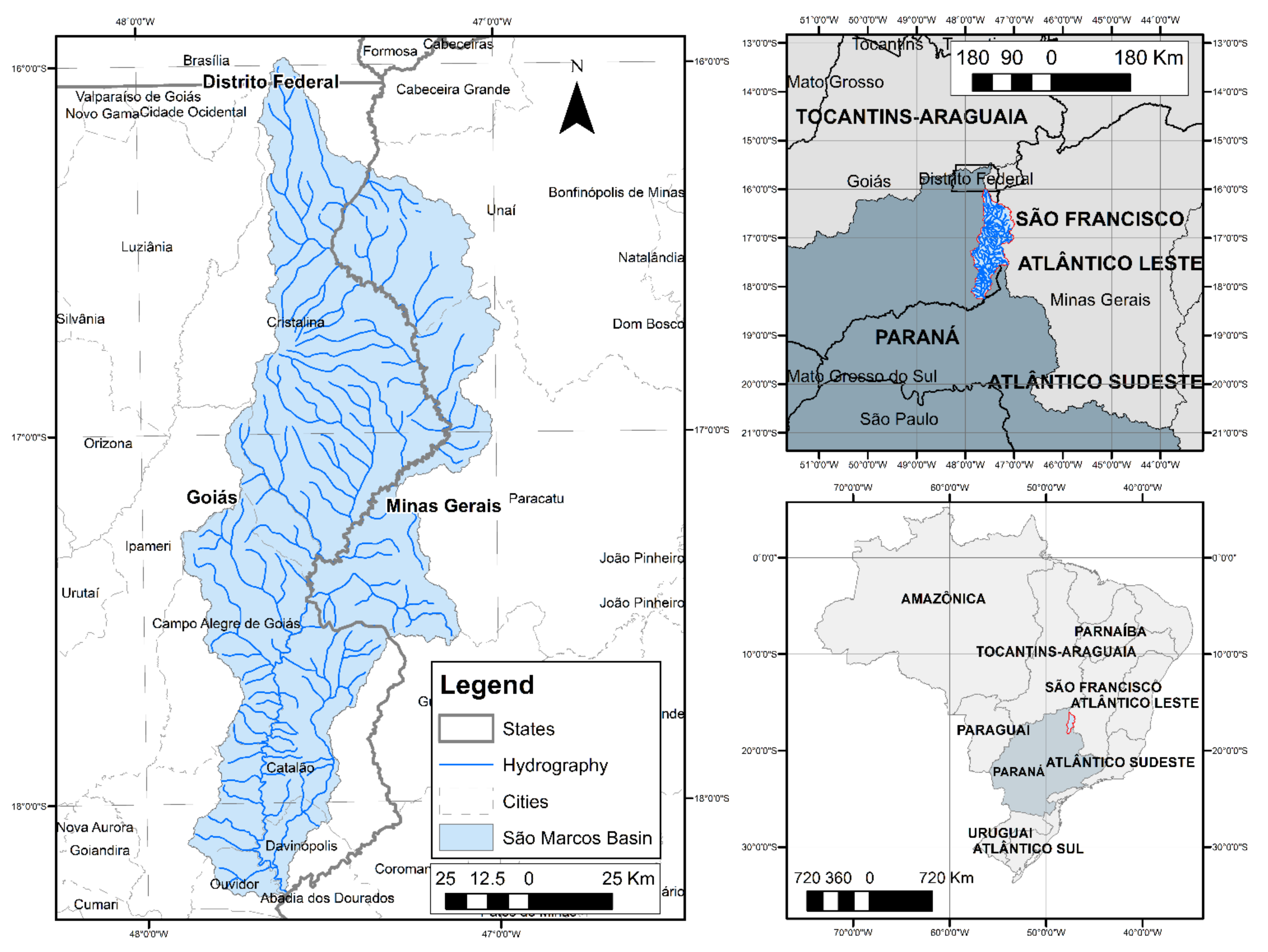
A brief description of the study area context is presented to explain the methodology and modeling analysis rationale. The study area is the São Marcos River Basin in the Paraná hydrographic region, Brazil (Figure 1).
The São Marcos River Basin occupies 1,214,000 hectares over two Brazilian states (Minas Gerais and Goias) and a small portion over the Federal District (DF). From this total, 96,874 hectares are irrigated with the center pivot method, standing out as the area with the highest concentration of pivots in Brazil [49,50]. The pivot’s average size is 87 ha, mostly new equipment operated by farmers with significant technological development [51]. The predominant crops are beans, maize, and soy, followed by others such as potatoes and garlic. The irrigation expansion in the region boomed starting in the 90 s, with the agricultural occupation of Brazilian savannas [52]. According to [53], irrigation with central pivots concentrates in some municipalities (e.g., Cristalina), which hold the largest agriculture production in the basin: garlic, coffee, beans, maize, soy, tomatoes, and wheat. The local economy relies heavily on the production chain resulting from agricultural production, with the municipality of Cristalina boasting a 36.5% population growth in 2000–2010 (48,463 inhabitants in 2013) and figuring as the Brazilian municipality with the highest Gross Added Value from agriculture in 2010 [54].
Irrigated agriculture data for the basin identified a total of 1132 central pivots, most of which located in the Sao Maros River affluents (state domain rivers) and supplied with small private reservoirs filled with water pumped from the rivers [52].
The watershed has two operational hydropower plants: Batalha and Serra do Facão, respectively, with 52.5 MW and 212.6 MW installed capacity. Batalha started operating in 2010, and Serra do Facão in 2014. For a powerplant to operate in Brazil, its project is issued a special water permit during the licensing phase, several years before entering operation, to secure the necessary water supply to produce the firm energy yield required by its concession contract. Both reservoirs are connected to the Brazilian Hydrothermal Power System, and the energy produced is allocated according to the system’s demand for loading and cost of energy production.
With the recent and significant increase in the region’s irrigated area, which took place mostly upstream of the hydropower reservoirs, water conflicts soon emerged. First conflicts were registered during 2010 by the brazillian National Water Resources Agency (ANA), involving hydropower operators and irrigators, most of the latter without formal water permits [52]. This issue was aggravated as the Goias state government fostered an irrigation development plan financed by the federal government to improve water infrastructure and support irrigation [52]. In response, the national water agency issued a technical note (No 104/2010) followed by a regulatory agreement with the states in the watershed (Resolution n° 562/2010) limiting water withdrawals upstream of the Batalha powerplant. However, as highlighted in [52], the Regulatory Agreement fell short on its effectiveness, as the states responsible for monitoring and overseeing water withdrawals from the São Marcos River affluents over their domain did not implement proper control on water uses. The combination of irrigators withdrawing without permits, as pointed in [52], limitations on water withdrawal overseeing, and increase in irrigation reduced the reliability in evaluating water availability for new water permits, which tend to overestimate supplies due to incomplete water use databases. All these issues tend to reinforce each other, resulting in an ongoing conflict in the region.
2.2. Methodology
The overall method is based on a Hydro-economic model developed with a stochastic dual dynamic programming (SDDP) approach [38]. The hydro-economic model runs under two different arrangements to determine economic benefits to the sectors in the watershed. The differences in economic benefits between these arrangements determine the tradeoffs, which consider hydrologic uncertainty and variability. The stochastic model’s main contribution to the results is to consider hydrological uncertainty, providing tradeoff information with an occurrence probability related to them.
The first arrangement—energy arrangement—represents exclusive hydropower use in the basin to evaluate this sector’s maximum potential benefits. This arrangement reflects the system’s original context when the hydropower sector had its inflows already secured through water permits and before the conflict with irrigated agriculture took place. Under this arrangement, the hydro-economic model allocates water to maximize the economic benefits from hydropower generation. Water is allocated following mass balance constraints, system topology, and water availability. There are no specific restrictions on user behavior, such as turbine minimum flow at hydropower plants (HPP’s) or minimum agricultural production, only availability and balance restrictions.
The second arrangement—economic arrangement—represents the existing hydropower in the energy arrangement, with current irrigated agriculture water demands added. Under this arrangement, the hydro-economic model allocates water to maximize the system’s overall economic benefit (sum of the economic benefits of electricity production and agricultural production). This arrangement reflects the context of both sectors sharing limited resources. Under this arrangement, the hydro-economic model maximizes the combined economic benefits (agriculture + energy), allocating water to each sector each month.
The results from both simulations include water flows and their marginal values, which vary in space and time according to hydrologic uncertainties. We then compare both arrangements to investigate the tradeoffs and economic benefits in the system, considering hydrologic variability. The latter aspect is important as hydrology variation may bring economic losses, which should not be mistaken by water allocated to other competing sectors. Those results focus on wetter hydrologic conditions (10% of exceedance probability) and drier conditions (90% of exceedance).
It is noteworthy that the purpose of this analysis is not to assess to whom the water should be allocated, nor to provide objective answers as to how water should be apportioned among these users, but rather to evaluate tradeoffs related to the different arrangements, which should be useful to support negotiations for conflict resolution and water allocation in the watershed. Water use priorities in Brazil are due to several legal, economic, social, and environmental factors, and the answer is not given by observing only one of these factors.
2.2.1. Model Data and Assumptions
The necessary data include irrigated agricultural use and power generation in the basin, financial and operational information of these uses, and hydrological characterization of the basin.
The model runs for a five-year period, where the first and last years are excluded to minimize the effects of boundary conditions in the results. The five-year run is necessary to obtain a steady-state solution to the optimization model, especially regarding reservoir operation. In the first year, it is affected by the influence of initial conditions and the system’s memory, and in the last year by the zero future water value. Hence, the most reliable results are obtained considering just the middle years.
In [55], a methodology is presented to estimate irrigated crops in a given area, considering the specific cycles and the agricultural calendar of the crops, and the available area, forming a spatial-temporal mosaic distribution of cropping. This mosaic gives planted area information for each crop each month, since the distribution is dynamic, to maximize the use of this area and economic benefits arising from agriculture. We adopted this methodology to estimate used space, assuming the irrigators would minimize the idle area and follow the region’s economic and cultural factors, keeping the crops of greater relevance. Monthly irrigation demands were then calculated from the estimated crop areas [55].
Reservoir and hydropower plant data were obtained from the geographic information system of the electric sector (SIGEL) of the brazillian National Electric Power Agency (ANEEL) [56]. ANEEL provides data regarding hydroelectric plants throughout the Brazilian territory. Technical and operational information on the reservoirs was obtained from the Brazilian electric potential information system (SIPOT) [57,58].
Inflows to hydropower reservoirs were obtained from the naturalized affluent flows series made available by the brazillian National Electric System Operator (ONS) [59]. Since ONS data are only available in reservoirs, flow time series were regionalized to be made available in other locations by area ponderation.
The model considers only two water uses: hydropower production and irrigated agriculture.
2.2.2. Hydro-Economic Model Formulation
The hydro-economic model employs a stochastic dual dynamic programming (SDDP) algorithm described in [60], and the specific implementation of SDDP used in this study is described in greater detail [38,61]. The algorithm runs on Matlab and uses the Gurobi solver.
The model will represent the two arrangements previously described (energy arrangement and economic arrangement) that will be compared to identify differences in economic benefits from water allocation and thus the tradeoffs. From these allocation results, it will be possible to tell where when, for what uses, and the probability of the water value, which will answer how one sector impacts the other, how much economic benefit it brings to the system, and its distribution among users, space, and time.
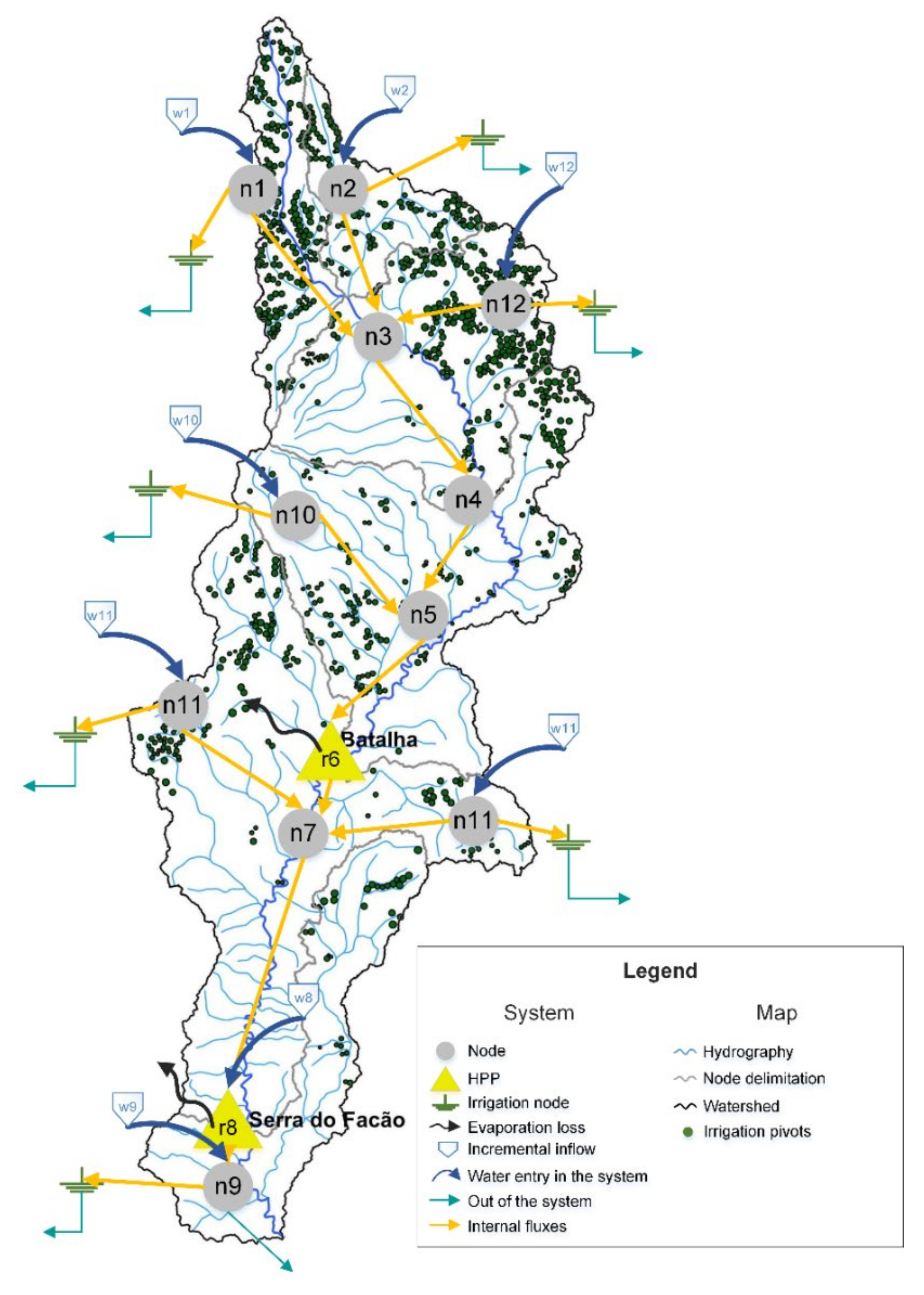
The model represents the elements of interest in the area, which include agricultural water demands, seasonality, and associated economic benefits, as well as other aspects of the water system, such as water flows, distribution, storage, naturalized flows, water demands, and associated economic benefits, storage infrastructure, evaporation and losses in irrigation systems and powerplants. A node and arc topology defining the São Marcos water system appears in Figure 2, with irrigated agriculture represented as irrigation demand nodes. Input data include irrigated area, maximum water demands for irrigation, reservoir information, and power plant energy generation information.
The model solves an optimization problem of water allocation, where the objective is to maximize the economic return of water use for irrigated agriculture and hydroelectric generation. However, the model’s goal is not to find an “optimal solution” for water allocation in the basin but rather assess upper bound benefits and then evaluate tradeoffs between the two sectors by comparing the two arrangements. In the actual system operation, identifying an “optimal” or even feasible water allocation would require a negotiation process among users and consider other aspects such as current allocation, access equity, and ecosystem demand, which are beyond this work’s scope. However, understanding the economic tradeoffs allows the designing of compensation instruments and can be useful as a starting point for negotiation.
Decision variables include reservoir releases, turbine flows for hydroelectric generation, and flows allocated to irrigated agriculture. The model is subject to physical constraints (storage capacity, turbine capacity, among others) and mass balance in each of the twelve nodes.
The model generates synthetic flows series from the observed series, allocating the available flows for the uses to generate the highest value, respecting the system’s mass balance restrictions. It extracts the marginal values of water varying in time and space and the total benefits generated in the system due to the objective function to maximize. Hydropower reservoirs operation is maximized by deciding turbine and released flows each month, thus affecting reservoir storage. When the model runs, it maximizes the total hydropower revenue by optimizing the operation of reservoirs and turbine flow and multiplying the average power produced by an energy price that reflects the marginal cost of producing one extra MWh in the Brazilian integrated power system, from [62].
Water for irrigated agriculture is allocated to each of 36 blocks representing six crops in six agricultural nodes. Water used in irrigated agriculture generates benefits based on production costs, productivity, and crop market price. If the demand is not fully met, productivity is reduced proportionally to the water deficit in the month of scarcity.
Agricultural production is based on crop water consumption values and a yield reduction factor (ky), which reduces production relative to water availability. From this production, the model generates economic benefits based on crop yields, fixed costs (R$/ha), production coefficient (ton/ha), and market value of the crop (R$/ton). Irrigation efficiency is considered 80% [55]. Of the remaining 20%, there is a 30% return efficiency to the downstream node [63], and 6% returns to the system.
As shown in Figure 2, nodes 1, 2, 10, and 12 represent irrigated areas at the head of the system (as irrigation demand nodes in the model), upstream of Batalha HPP. Node 11 represents the irrigated areas upstream of Serra do Facão HPP (and downstream of Batalha HPP), and node 9 represents the irrigated areas in the final stretch of the system, downstream of both HPPs.
2.2.3. Solving the optimization problem through stochastic dual dynamic programming (SDDP)
General Description
We solve a multi-reservoir operation problem to find the optimal operational path of water storage and releases, accomplished by maximizing the sum of the present and future benefits from the releases for power generation and irrigated agriculture. Future benefits depend on water storage in the reservoir and future uncertain inflows. Since storage depends on the present release decisions, decisions are coupled in time. Thus, the model solves a stochastic multistage problem with temporal coupling and nonlinear benefit functions. The general formulation of a multistage optimization problem is given by (1) [61].
where
- is the expectation operator;
- is the index of time (month);
- is the last time period (month);
- is a discount factor for the value of economic benefit over time;
- is the benefit function at stage t (R$);
- is a vector of storage at time t (hm3);
- is the allocation vector (decision variables: turbine, flow) (hm3);
- is the affluent flows vector (hm3);
- is a terminal value function that estimates the value of de at time period T (R$);
Equation (1) is the objective function that maximizes total economic benefit and Z the total expected benefit in t = 1, 2, 3,…, T
Subject to constraints (2), (3) and (4):
where C is a connectivity matrix linking different elements in the network, and the other variables were presented above.
The stochastic dynamic programming (SDP) version of the above optimization problem is defined by Bellman’s Equation (5).
where is a maximization operator. The remaining variables were presented above.
However, the SDP solution for this problem requires discretization of the entire state space (all values of S and q), making the computational cost of the problem excessively large for a larger number of state variables. Several techniques are proposed in the literature to overcome this limitation. We adopted the stochastic dual dynamic programming approach (SDDP), which can create a locally approximated future benefit function by employing successive extrapolations constructed from the dual variables of the stochastic optimization problem [42]. Several of the optimization methods employed by the national system operator (ONS) in Brazil make use of SDDP algorithms.
The SDDP algorithm also uses an analytical representation of hydrological uncertainty that limits the computational effort required to solve the optimization problem by preventing discretization of the hydrological state variable. A set of synthetic flow series is used to simulate the system and check the approximation of future benefit functions. A more detailed description is presented in [38].
The economic benefits from hydropower generation are a function of the energy generated and the price of energy in the month the flow is turbined. The values are calculated considering the marginal value of energy in the Brazilian hydrothermal system.
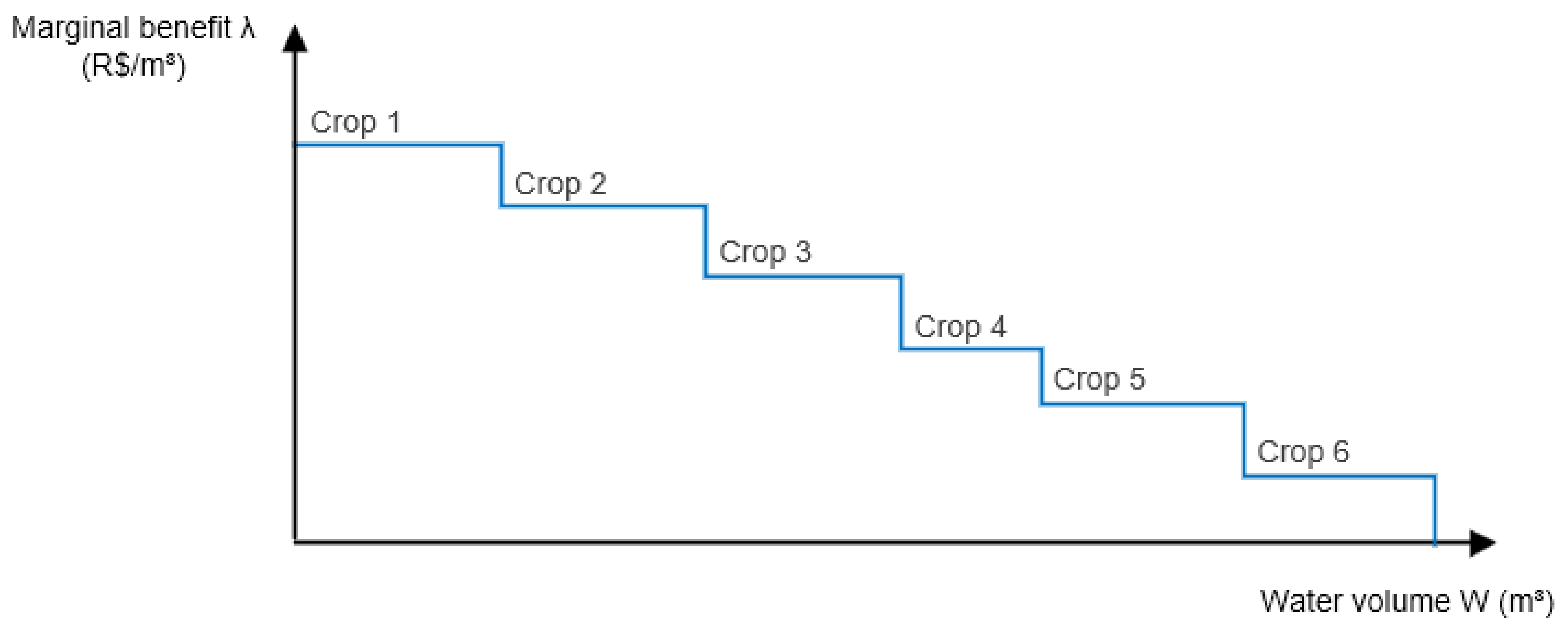
In a given period, additional water has different values from the previous ones as they are allocated to different crops, which yields a marginal value curve similar to that observed in Figure 3.
Irrigation data from the Brazilian Institute of Geography and Statistics (IBGE) regarding agriculture patterns in each municipality of the watershed allowed the identification of the most common crops and their location. From this, typical central pivot irrigated crops that are more representative of the area were selected. Given the historical characteristics of the region’s crops, soybean, maize, garlic, beans, coffee, and potato were selected as the most representative crops for the region. Each crop is modeled with a constant productivity function (kg/m3); however, as the crop mix varies between different crops and across the regions, the marginal water benefit (and thus the marginal willingness-to-pay for water) varies across the irrigation regions, depending on the location and period of the year.
Model Output
For the São Marcos system, the model has 15 output variables, 12 nodes, and 60 months, which would generate 345,600 results. Some of the variables are discretized into more or less than 12 nodes (such as variable i, discretized in 36 blocks, or variable ib, which refers to the whole system).
Each model run is done for a 60 month horizon, using 30 sequences of inflows generated internally by a multisite periodic autoregressive (MPAR) model. Thus, for each output variable at each point of the system, the model produces 30 time series of 60 months duration resulting in 30 probabilistically possible series, one for each possible sequence of inflows qt. These results are organized into exceedance probability curves, relating the values to a probability of occurrence. This allows analysis of the probabilities and uncertainties regarding the value of economic benefits and tradeoffs. We analyzed results from the exceedance probability curves generated in wetter (10% of exceedance probability) and drier conditions (90% of exceedance).
The Lagrange multiplier (λ) associated with the mass balance equation represents the marginal value of water, which corresponds to the increment in the model’s objective function resulting from an additional unit of water at a given point and time. This increment is an estimate of the economic value that an additional unit of water would add to the system, at that point, at that time. This variable also represents the marginal opportunity cost of water, indicating the economic benefit that could be produced if an additional unit of water were reallocated from another point in the system to the point in question. In the representation of the system, a point is represented by a node, which can be a reservoir or a demand node.
The four result sets are summarized in Table 1.
3. Results and Discussion
3.1. Energy and Economic Arrangements
The frequency distribution for the average economic benefits under both arrangements appears in Figure 4 for monthly economic benefits generated (R$1,000,000.00) in the São Marcos HPP system. The separation between both curves indicates economic tradeoffs to energy due to reduced inflows, as water is shared with irrigated agriculture. The spread in the curves indicates natural hydrological variability and probability of occurrence.
Comparing the economic arrangement with the energy arrangement indicates that the total hydropower benefits are reduced by 5.64% (R$27 million per year) for the 90% exceedance dry scenario and 4.62% (R$29.6 million per year) for the 10% exceedance wet scenario. The absolute deficit is higher in the 10% scenario because of the higher water availability. In relative terms, however, it is lower because since agriculture is favored in the optimization, it uses a similar amount of water in both scenarios, so the absolute impact it has on energy generation is similar.
If we consider the losses caused by water availability changes, hydropower loses R$162.4 million/year due to less available water, which represents 25.31% of the total benefit in 10% of the years. That absolute loss decreases to R$159.8 million/year (representing 26.11% of the total benefit) in the economic arrangement. Table 2 presents the average annual benefit generated for the two hydropower plants’ optimized operation in the basin.
Figure 5 shows water withdrawals to the irrigated uses in the six demand nodes of the system (hm3), under the economic arrangement, with 90% (a) and 10% (b) exceedance probability. The largest water withdrawals during the dry years (90% exceedance) take place in July/August at nodes 12 (Minas Gerais Irrigation), followed by 10 (Consumo Batalha), which are both upstream of both hydropower reservoirs (Batalha and Serra do Facão). Further downstream, between the hydropower plants, irrigation demand node 11 (Consumo Serra do Facão) is also significant. Another irrigation node far upstream, node 1, has low withdrawals, likely due to localized scarcity.
However, 10% of the time, during the wetter years, irrigation withdrawals are higher for several nodes (the highest at node 10), including node 1 (Rio Samambaia) farther upstream. The latter, likely due to improved local water availability conditions. Node 1 also has higher water withdrawals in July (rather than June in the dry years), indicating a possible shift in the crop calendar.
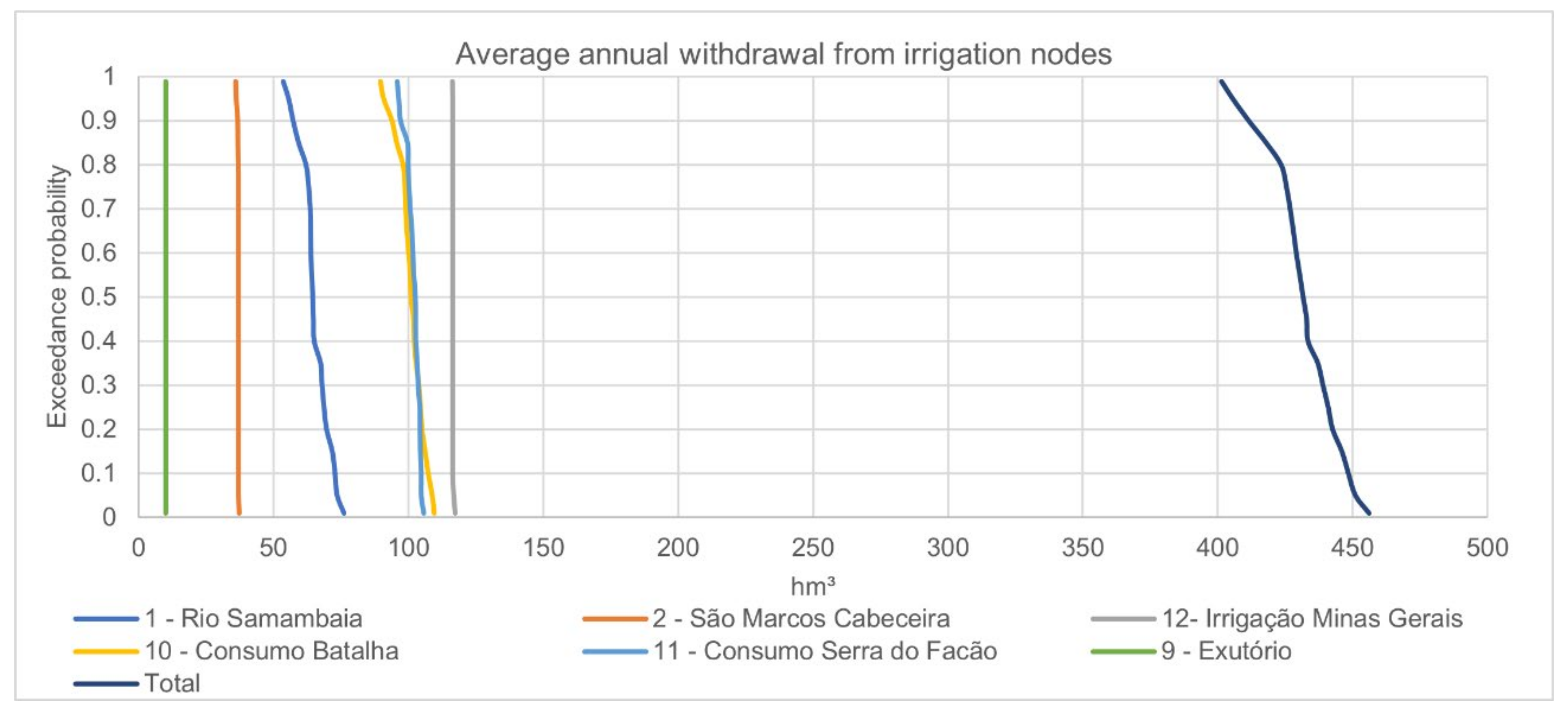
Figure 6 shows the exceedance probability curves for the average annual water withdrawals at the irrigation nodes and the system. The variation between exceedance probabilities indicates a deficit to meet the total demands caused by hydrological variability (if 100% of the demands were met, the hydrological variability would not impact the withdrawal flow). Some demands like node 2 (São Marcos Cabeceira, which is not exceptionally large compared to the others) present a nearly vertical line, indicating that most of the demand is met almost all the time. The same with node 12.
Table 3 shows the actual evapotranspiration and water demands for irrigation and the water withdrawals for both scenarios and the six irrigation nodes. Of the total water demand (549.7 hm3/year), 411.6 hm3/year is met 90% of the time (138.1 hm3/year deficit), and 448.4 hm3 in 10% of the time (101.2 hm3/year deficit). Node 1 (Rio Samambaia) responds for most of this result, as its demand is significant (19.3% of the system total demand), and it faces a deficit up to 48.9% in the drier years (90% exceedance probability). One-third of Rio Samambaia’s demand (33.3%) is still not met even in the wetter 10% years. This result indicates that even under favorable hydrological conditions, the upstream nodes concentrate a deficit (water scarcity). This watershed region has smaller drainage areas with reduced flow rates, and water cannot be allocated here from other points of the system.
Overall, the results indicate that irrigated agriculture received water allocation capable of supplying 75% of its demand 90% of the time and 81% in 10% of the time. This means an approximate water supply deficit of 19% to irrigated agriculture, even in the wetter 10% years.
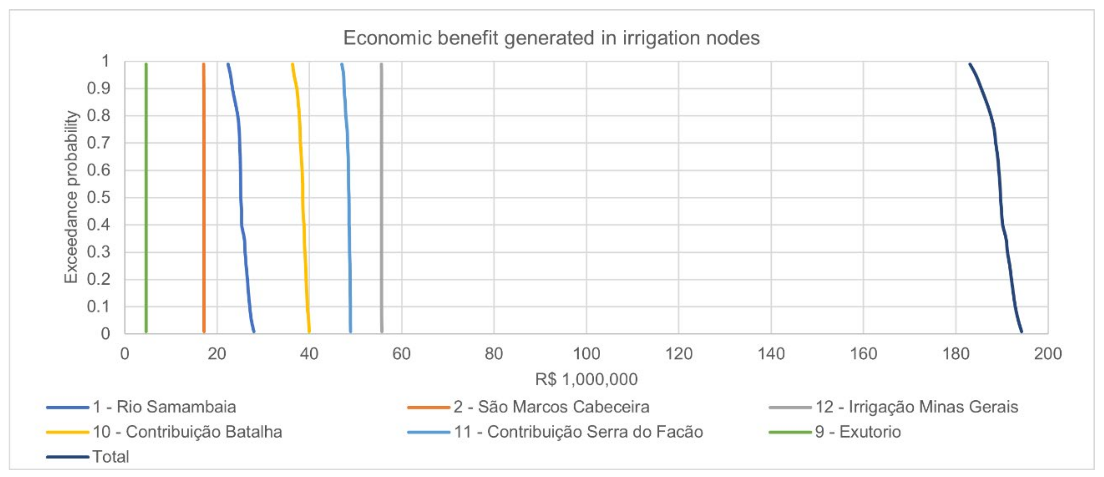
The economic benefits generated by irrigated agriculture are presented in Figure 7 shows exceedance curves for the average annual benefits generated by irrigated agriculture at irrigation nodes.
As expected, the hydrological variability reflects on economic benefits, as presented in Table 4, for the 90% and 10% exceedance scenarios. If all irrigated agriculture demand is fully supplied (549.7 hm3/year), the maximum economic return is 202 R$ million/year. Hence, the 19% water supply deficit verified in the previous section represents a 4.5% drop in economic benefits in the 10% exceedance scenario (R$9.08 million) and a 5.15% drop in the 90% exceedance scenario (R$16.47 million).
The differences in economic benefits in Table 4 reflect some of the hydrological variability, which can reduce the benefits by at least R$7.38 million/year, comparing the more favorable conditions (10% of exceedance) with less favorable conditions (90% of exceedance). This difference is equivalent to 3.83% of the whole benefit in the 10% exceedance scenario, considering the whole system. This difference is not uniform in the system. Table 4 shows that most of the economic benefits are concentrated upstream of Batalha HPP, in nodes 1, 2, 12, and 10 (R$6.06 million, or 19.76% of what is generated in those nodes). The Rio Samambaia (node 1) is subject to a variation of R$3.70 million, equivalent to 13.67% of its benefit in the most favorable years (10% of exceedance probability) and almost half of the difference in the whole system. Downstream of the reservoirs, nodes 11 and 9, benefits from the regularization effect and have smaller differences. Nodes 2 and 12, however, are upstream and have a small difference as well. One possible explanation is the value of production in these regions, associated with local water availability differences.
3.2. Marginal Water Values
This section presents the marginal value of water in the nodes, presented in monthly and average values (R$/1000 m3). Marginal water values are obtained from the Lagrange multiplier associated with the water mass balance equation in the hydro-economic optimization model in each node of the system, indicating the potential increase in the objective function value (economic benefit) if one extra 1000 m3 of water was available at the specific location and time.
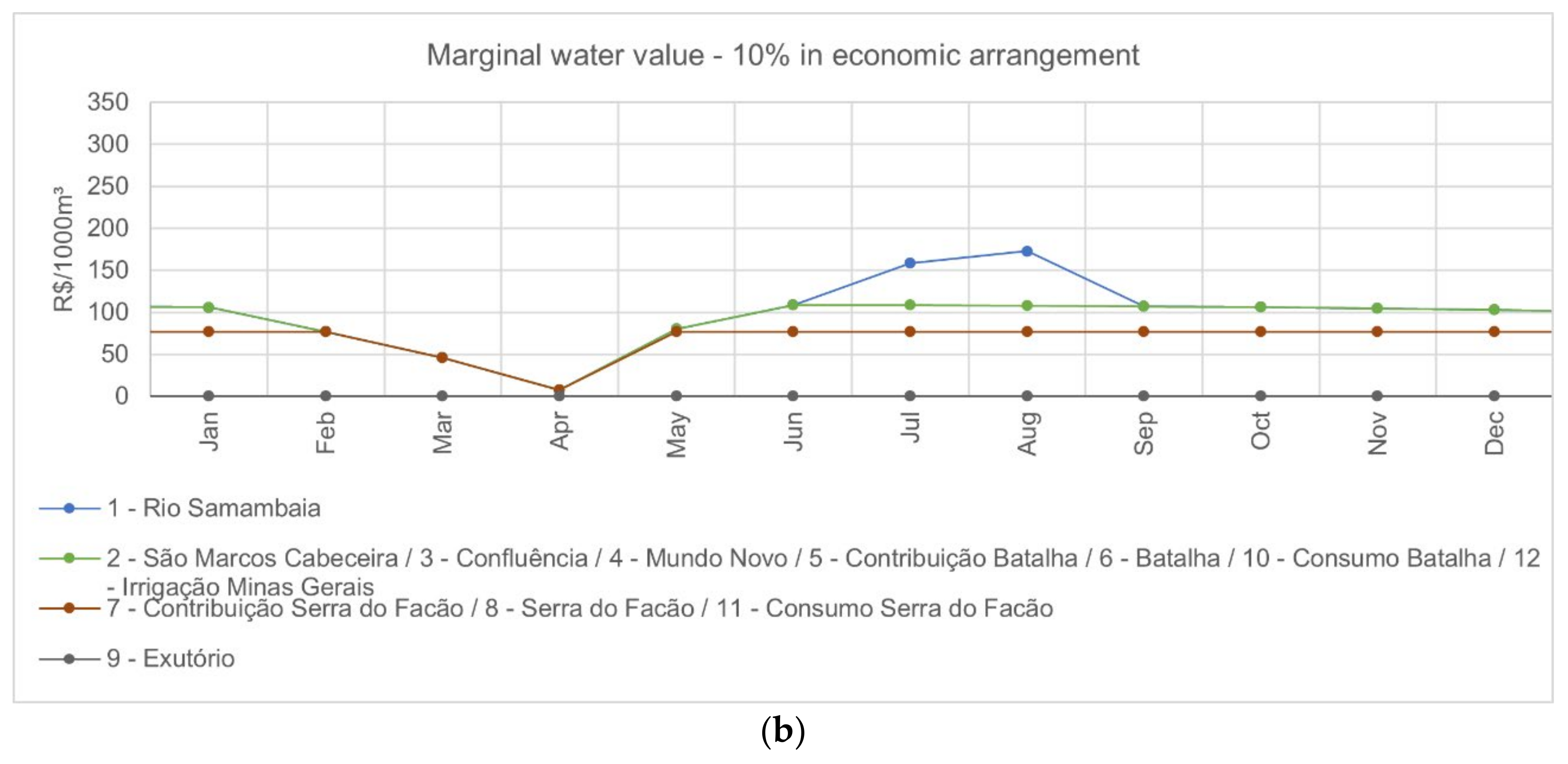
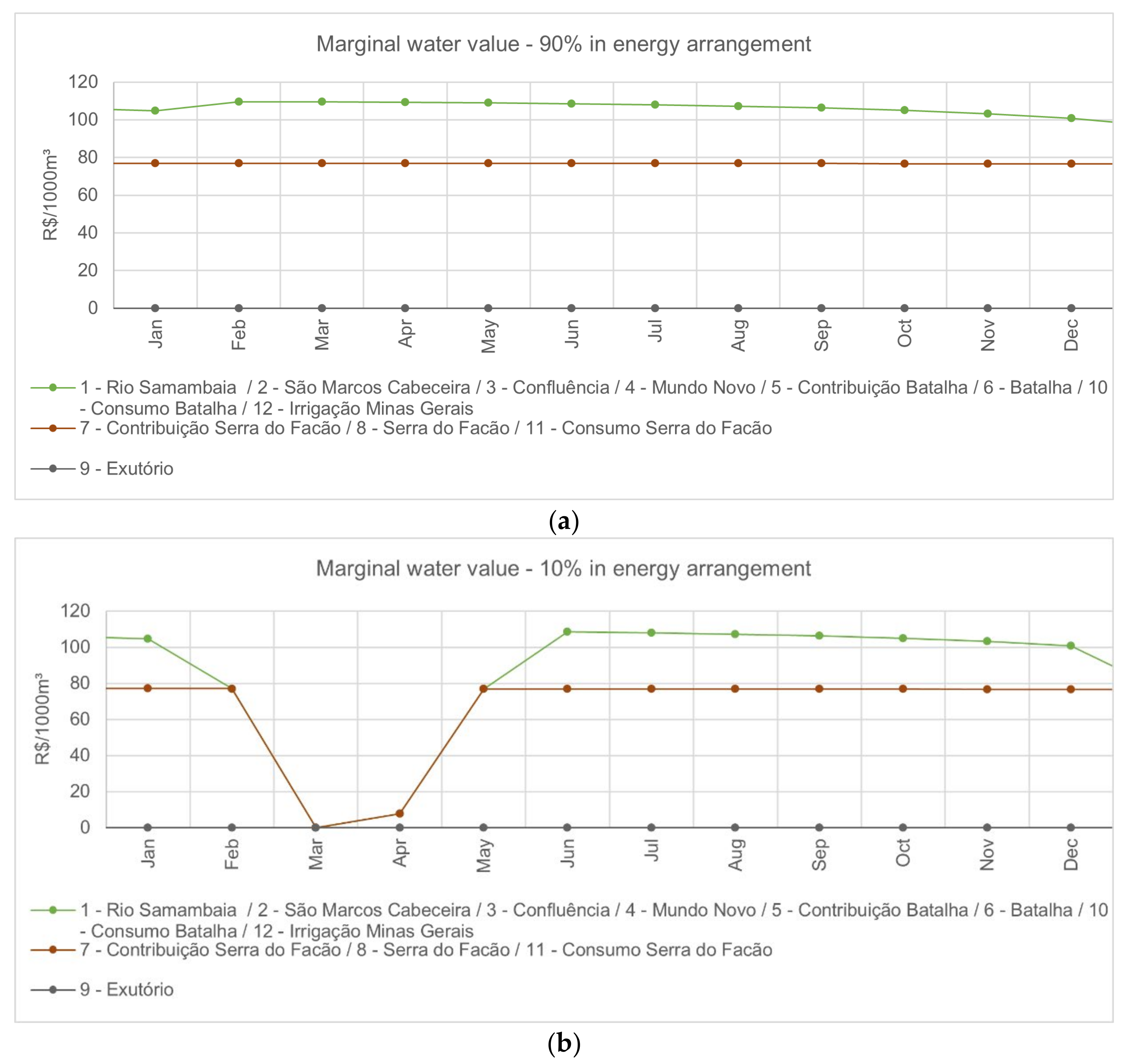
Figure 8a,b and Figure 9a,b present the time-series of marginal values for the two arrangements (energy and economic) and the two scenarios (90% and 10% of exceedance probability). The marginal value is zero when there is no benefit to be gained from an extra unit of water (i.e., water constraint in the mass balance equation is slack), and it increases with water scarcity. Marginal values in node 9 (Exutório) are zero since uses from this point onward are not modeled. The marginal value peaks reflect the high water demand during the irrigation season. As expected, the values are overall higher in the dry years (90% exceedance probability) than in the wet years (10% exceedance probability).
Under the economic arrangement, for the 90% exceedance scenario (dry years), the peaks reached R$0.30/m3 to irrigated agriculture. In contrast, node 1 (Rio Samambaia) presented the highest values (from June to August) due to its upstream location and small drainage area. August is also the month when the marginal values peak for all demands. As the scarcity reduces as we move to downstream regions, so do the marginal water values. At the upstream nodes (mainly 1 and 10, with one peak at node 11), the marginal values of water range from R$0.07/m3 to R$0.11/m3. Over the remaining months, there is a reduction from January, extending to March. These are months when the demand is the lowest due to the rainy season. For the dry years in the economic arrangement, some periods presented zero marginal value, indicating demands were met.
In the energy arrangement, the marginal water values are mostly invariable throughout the year, reflecting the energy values and water access. In the wet years, however, marginal water values in March and April were close to zero, indicating abundant water supplies with full reservoirs and turbines running at maximum capacity, achieving the nominal power of the HPP.
Comparing the magnitude of the values between the economic and energy arrangements indicates the increment brought in by irrigated agriculture in the region. For example, in August during the dry years, the upstream region (nodes 1 through 12) has water at approximately R$0.105/m3 if hydropower was the exclusive demand in the basin (energy arrangement), while when agriculture is added, the economic marginal water value raises threefold, up to R$0.30/m3.
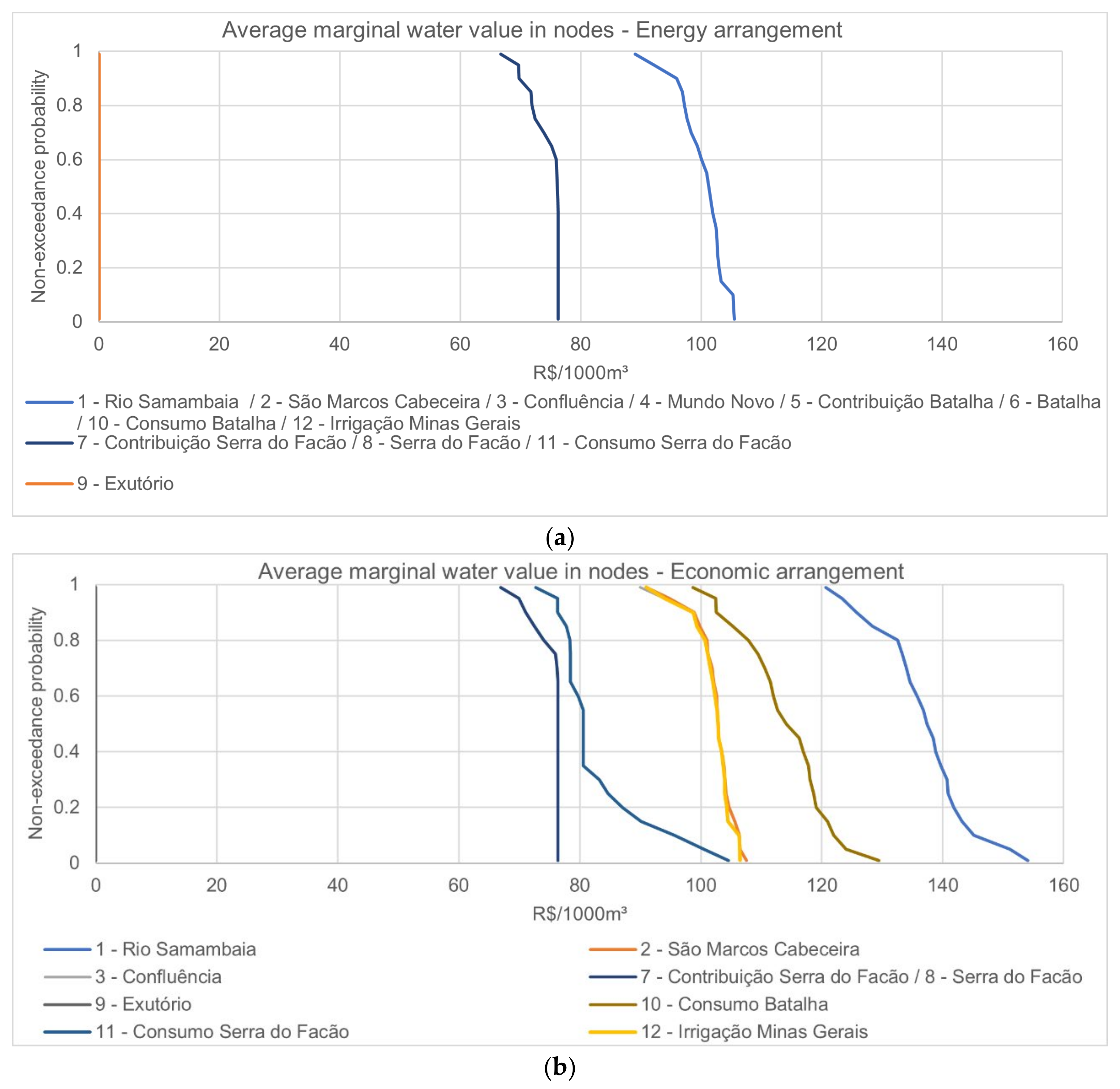
Figure 10 presents the non-exceedance curves for yearly average marginal values for the economic and energy arrangements. In the non-exceedance curve of average values, it is possible to observe where water is scarcer (i.e., it has a higher marginal value), in decreasing order, from upstream to downstream.
The only values presented in non-exceedance probabilities are the marginal values, which are inversely proportional to the availability of water. This means that the 0.9 non-exceedance probability (low marginal values) is equivalent to the 0.1 exceedance probability for the other variables (high water availability).)
The curves overlap at some nodes, where the marginal value is the same. In the energy arrangement, three curves are observed at Batalha, Serra do Facão, and the Exutório nodes, indicating that water used only for hydropower purposes has the same value anywhere upstream of Batalha (curve 1/2/3/4/5/6/10/12) or downstream of Batalha and upstream of Serra do Facão (curve 7/8/11). The overlapping of curves is also observed in the economic arrangement, however, with more dispersion in the values, as water can be allocated to different crops with different economic returns.
These values indicate the potential for generating economic benefit from the two water uses in the basin and the water use rivalry. As seen in Table 5, when irrigated agriculture is included in the system (economic arrangement), the marginal water values increase compared to the energy arrangement. This shows that, while hydropower may have significantly smaller consumptive use (i.e., mostly evaporation), both uses compete for water due to the timing of the releases when reservoirs operate to maximize hydropower production.
As higher scarcity and marginal values are observed at upstream nodes, it would be economically more efficient to concentrate irrigated agricultural uses downstream of the HPP’s, to use water in irrigation after generating power. However, due to other reasons (e.g., soil fertility, availability, and social causes), the basins’ headwaters are precisely where most of the central irrigation pivots are concentrated.
3.3. Total Economic Benefits and Tradeoffs
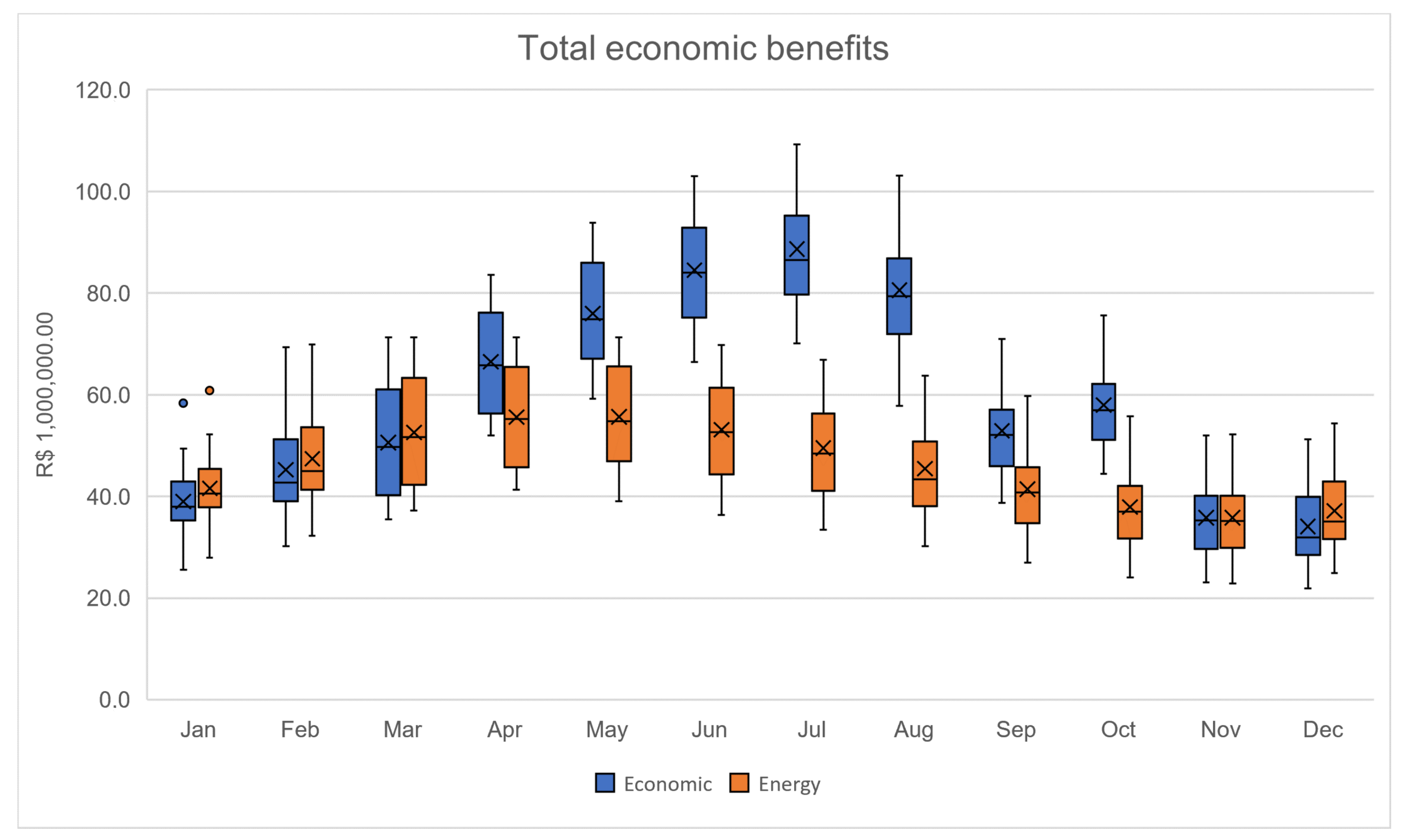
Hence, far, changes in energy generation and irrigated agriculture were analyzed. Still, the full tradeoff analysis also involves the gains for the irrigated agriculture sector and the system as a whole. Figure 11 shows the benefits generated each month for the two scenarios and allocation arrangements.
As agriculture shares water with hydropower, a clear gain in total economic benefits is perceived from April through October, the dry months where irrigation is concentrated. There is no perceivable change in the dispersion of the total benefits throughout the years. Some tradeoffs are present from December to March, due to more water available to hydropower, without consumptive irrigation use.
When hydropower is the exclusive water demand (energy arrangement), power production and benefits rise after November and peak in April. When irrigated agriculture is considered (economic arrangement), total benefit peaks later in July, following the agriculture calendar. Overall, the presence of irrigated agriculture in the economic arrangement outweighs the tradeoffs.
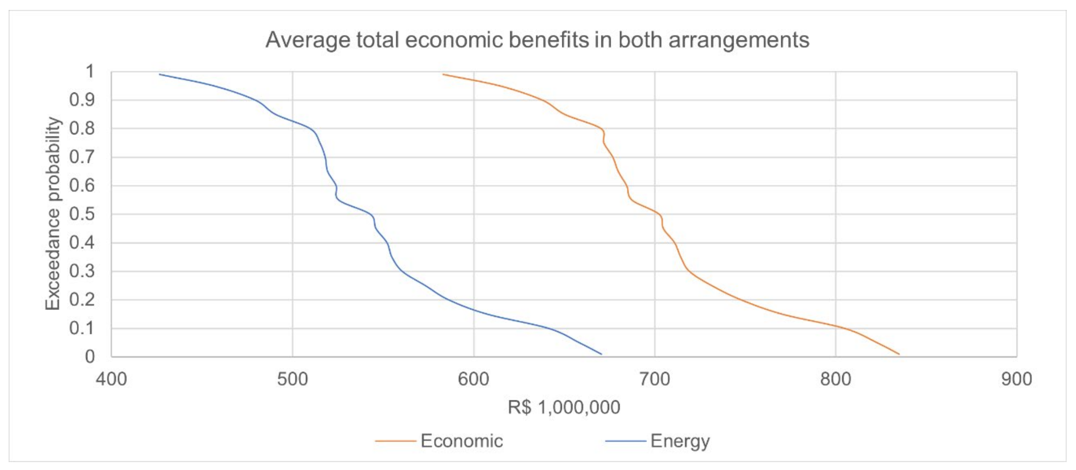
Figure 12 shows the exceedance curves for average annual total benefits generated in the system.
Table 6 shows the total benefits for the 90% and 10% scenarios and allocation arrangements. The energy sector would produce a benefit of R$479.3 million/year 90% of the time if it had exclusive access to water to maximize hydropower production and reach up to R$641.7 million/year 10% of the time in the wet years. As water is shared with the irrigated agriculture sector, the energy benefits are reduced to R$452.3 million/year, resulting in a R$27 million/year tradeoff in energy benefits 90% of the time.
However, the irrigated agriculture sector also brings in R$185.5 million/year in economic benefits as it receives water allocation. Discounting the energy benefit tradeoff, the net gain to the water system is R$158.5 million/year (90% of the time), and it could still reach up to R$163.3 million/year in the 10% wetter years.
Table 7 compares the economic tradeoffs resulting from the different arrangements and scenarios.
While irrigated agriculture benefits outweigh the potential energy losses, in the 10% exceedance scenario, the energy loss is slightly higher, at R$29 million/year, as the water surplus is directed to agricultural uses, which have a higher marginal water value.
The total system economic benefits generated by the two sectors in the basin vary from R$637 to R$805 million per year (US$208.01 million, considering US$1.00 = R$3.87, in December 2018), being higher for the energy sector, which under favorable water conditions (10% scenario) can produce R$612.1 million/year (US$158.17 million), which is equivalent to 76% of the total economic benefit generation in the basin. Under the same conditions, agriculture’s economic benefit contributes to a total of R$192.9 million/year (US$49.84 million), which is equivalent to approximately 14% of the total benefit. Generated and lost benefits are larger in the 10% exceedance scenario because of the larger amount of water involved, with the higher flows related to the wetter scenario.
The total system average unitary economic benefit (i.e., total benefit divided by the amount of water applied in production (water withdrawals for irrigated agriculture and turbine flows for hydropower), in R$/m3 average) peak at R$0.43/m3 (US$0.111/m3) to R$0.451/m3 (US$0.0117/m3) in the 10% and 90% exceedance scenarios, respectively, for irrigated agriculture. For hydropower generation, the values range from R$0.038/m3 (US$0.0098/m3) to R$0.039/m3 (US$0.0101/m3) for the Batalha HPP, and R$0.093/m3 (US$0.024/m3) to R$0.096/m3 (US$0.025/m3) for the Serra do Facão HPP, which result in total unit benefits, considering the cascade of reservoirs, from R$0.127/m3 (US$0.033/m3) to R$0.135/m3 (US$0.035/m3). This relates to the value obtained in a previous study [64] of R$0.13/m3 for the average unit value of water in the cascade of hydroelectric power plants from Batalha to Itaipu hydroelectric power plant. For irrigated agriculture, the values obtained by ANA [64] were around an average profit of R$0.35/m3 (US$0.09/m3). Values obtained by [54] show that the region produces an average revenue of R$14,699/ha (US$3798.19/ha) in irrigated agriculture, compared to an average profit of R$1915/ha (US$494.83/ha) to R$1991/ha (US$514.4/ha), depending on the hydrological scenario, obtained in our results.
Energy generation also brings other benefits not quantified here, for example, the contribution to decreasing energy price throughout the integrated national electric system, energy security, and additional downstream hydropower plants energy generation, which depends on São Marcos River HPP operating decisions (going as far as Itaipu, on the Paraná River). On the other hand, the irrigated agriculture sector also has other benefits resulting from income and employment multiplier effects throughout its production chain. Takasago et al. [65] points out a total income multiplier of R$612,199 (US$158,191) per change in final demand of one million reais and a total employment multiplier of 60.36 jobs per change in final demand of one million reais.
A similar study comparing agriculture and energy sectors with an SDDP model [48] reached a different conclusion, suggesting allocating to the energy sector in some river basins due to higher marginal water value on the sector. This demonstrates that tradeoff information between water uses is not always evident, and specific assessment is necessary to acquire that kind of information.
The magnitude of the marginal water values can be compared to the values of water charges (economic water management instruments) to Brazil’s agricultural sector. Typically, water charges implemented in Brazilian river basins either exempt or guarantee differentiated payments to the agricultural sector, with values that hardly exceed one cent per cubic meter, on the justification that it is a sector with low added value generation and that higher water charges would make the activity unfeasible. Our results indicate it is not always the case, given that the marginal values of water reached values up to R$0.30/m3 (US$0.078/m3) in specific months and around R$0.10/m3 (US$0.026/m3) most of the time. This indicated that values around R$0.10/m3 would not be necessarily prohibitive for the sector’s operation, considering the characteristics presented here.
Finally, direct comparisons between benefits generated per unit of water (R$/m3) between these two sectors must be made with reservations. The demand for agriculture makes a consumptive use of water, making it unavailable quantitatively or qualitatively for other users. The impact on availability caused by power generation is often due to water storage, water releases (although there are evaporation losses, they are small compared to flows captured for agriculture) and are considered positive when provides a downstream flow regularization service. If the same agricultural water demand were located downstream of hydropower uses, the benefit generation could be similar (considering other factors such as soil fertility and topography invariable), without reduced tradeoffs to hydropower. A similar conclusion was reached in [32], where irrigated crop revenue could be raised by 49%, and reducing crop losses during droughts by 30% if reservoirs supplied irrigation through flow regularization.
4. Conclusions
The following specific conclusions are possible, addressing the three key points of investigation proposed in the beginning:
How much benefit could the energy sector potentially lose when water is shared economically with the agriculture sector? Losses can reach up to 4.6% in hydropower benefits (R$29.6 or US$7.65 million/year), but 90% of the time, losses are around 5.6% (R$27.0 or US$6.98 million/year).
How much benefit does the agricultural sector bring into the system when water is shared with the energy sector? System benefit can increase up to 29% (R$185.5 or US$47.93 million/year) 90% of the time.
How likely are these benefit changes, considering hydrologic variability and competition for water? Total system benefits can vary approximately 26.1% between dry and wet years. Hydrologic variability also responds for a 3.8% change in irrigated agriculture benefits and 25.3% in hydropower benefits due to lack of water availability in drier years. When hydropower and irrigated agriculture share water allocation, the variation in hydropower benefits increases to 26.1%. Hence, agriculture brings an additional 0.8% relative variation in the hydropower benefits, which is an added risk.
In general, we also conclude the following main points, which are relevant for the discussion and negotiation on water allocation and conflict resolution:
- While the water–food–energy nexus brings in tradeoffs from water allocation in the watershed, the overall result can be positive, as is the case in the modeled system. The energy generation is often perceived as a much higher value, but irrigated agriculture can reach significant values as well;
- The location and water allocation to the demands affect the tradeoffs. In the system modeled, water has been overallocated upstream of the powerplants, which makes the problem more difficult to address;
- As the agricultural benefits outweigh the potential energy losses in the modeled system, the best course of action is to find an economically compensated reallocation strategy, upon negotiation among users, rather than imposing water supply cutbacks to the agriculture sector. The tradeoff values presented here are useful information to negotiate those strategies among irrigators and power companies;
- Hydrologic variability is responsible for some benefit losses, especially upstream in the system where water is scarcer;
- There is already a great deal of hydropower revenue variation even without irrigation demands, and sharing water with irrigation further increases this risk.
- The variation in irrigated agriculture economic benefits is comparatively smaller by one order of magnitude than the variation in hydropower benefits. As irrigation receives water first and its water demand is relatively smaller, it is less affected by hydrologic variability;
- The economic value of water varies over time and space, which indicates users’ availability to pay or to be compensated for water considering its scarcity in different months, hydrological scenarios, and places. This is a starting point for a negotiated allocation process capable of signaling to current and future users the spatial location and the demand pattern that can be accommodated in the basin, depending on the economic value of the water;
- The variability in the water’s economic values reflects the hydrological variability in the basin itself (combined with water use and storage operations). It can be used to better understand the risks associated with decisions taken from the negotiated allocation. This aspect is still little explored by the management of water resources in Brazil, but it contributes to give more transparency in the information process to the parties involved in the negotiation process. Knowing the likelihood of making a given amount of water available for reallocation, as well as how much it would cost in compensation, allows for better planning by those involved.
Author Contributions
Conceptualization, P.H.B., G.F.M. and A.T.; methodology, P.H.B. and G.F.M.; software, A.T.; validation, P.H.B., G.F.M., A.T., A.P.D. and M.O.; formal analysis, P.H.B. and G.F.M.; investigation, P.H.B. and G.F.M.; resources, G.F.M.; data curation, P.H.B.; writing—original draft preparation, P.H.B. and G.F.M.; writing—Review and editing, P.H.B., G.F.M., A.T., A.P.D. and M.O.; visualization, P.H.B., G.F.M., A.T., A.P.D. and M.O.; supervision, G.F.M. All authors have read and agreed to the published version of the manuscript.
Funding
This research was supported by CNPq Grant No. 201185/2011-3 and CAPES Grant No. 88881.065004/2014-01.
Institutional Review Board Statement
Not applicable.
Informed Consent Statement
Not applicable.
Data Availability Statement
Reservoir and hydropower plant data available in the geographic information system of the electric sector: http://sigel.aneel.gov.br (accessed on 8 November 2020). Naturalized inflows to hydropower reservoirs available in the national electric system operator (ONS) website: http://www.ons.org.br/ (accessed on 8 November 2020). Central pivots data available in: https://metadados.snirh.gov.br/geonetwork/srv/por/catalog.search#/metadata/e2d38e3f-5e62-41ad-87ab-990490841073 (accessed on 8 November 2020).
Acknowledgments
The authors thank IPH/UFRGS, CNPq and CAPES for their support in this study.
Conflicts of Interest
The authors declare no conflict of interest.
References
- Carvalho, R.C.D.; Magrini, A. Conflicts over Water Resource Management in Brazil: A Case Study of Inter-Basin Transfers. Water Resour. Manag. 2006, 20, 193–213. [Google Scholar] [CrossRef]
- Ioris, A.A.R. Water Resources Development in the São Francisco River Basin: Conflicts and Management Perspectives. Water Int. 2001, 26, 24–39. [Google Scholar] [CrossRef]
- De Penteado, C.L.C.; Almeida, D.L.; Benassi, R.F. Conflitos hídricos na gestão dos reservatórios Billings e Barra Bonita. Estud. Av. 2017, 31, 299–322. [Google Scholar] [CrossRef] [Green Version]
- Getirana, A.C.V.; de Malta, V.F.; de Azevedo, J.P.S. Decision Process in a Water Use Conflict in Brazil. Water Resour. Manag. 2008, 22, 103–118. [Google Scholar] [CrossRef]
- Hess, C.E.E.; Fenrich, E. Socio-Environmental Conflicts on Hydropower: The São Luiz Do Tapajós Project in Brazil. Environ. Sci. Policy 2017, 73, 20–28. [Google Scholar] [CrossRef]
- Amorim, A.; Ribeiro, M.; Braga, C. Conflitos Em Bacias Hidrográficas Compartilhadas: O Caso Da Bacia Do Rio Piranhas-Açu/PB-RN. Rev. Bras. Recur. Hídr. 2016, 21, 36–45. [Google Scholar] [CrossRef]
- Wild, T.B.; Reed, P.M.; Loucks, D.P.; Mallen-Cooper, M.; Jensen, E.D. Balancing Hydropower Development and Ecological Impacts in the Mekong: Tradeoffs for Sambor Mega Dam. J. Water Resour. Plan. Manag. 2019, 145, 05018019. [Google Scholar] [CrossRef]
- Yang, Y.C.E.; Ringler, C.; Brown, C.; Mondal, M.A.H. Modeling the Agricultural Water–Energy–Food Nexus in the Indus River Basin, Pakistan. J. Water Resour. Plann. Manag. 2016, 142, 04016062. [Google Scholar] [CrossRef]
- Mercure, J.-F.; Paim, M.A.; Bocquillon, P.; Lindner, S.; Salas, P.; Martinelli, P.; Berchin, I.I.; de Andrade Guerra, J.B.S.O.; Derani, C.; de Albuquerque Junior, C.L.; et al. System Complexity and Policy Integration Challenges: The Brazilian Energy-Water-Food Nexus. Renew. Sustain. Energy Rev. 2019, 105, 230–243. [Google Scholar] [CrossRef]
- Mushtaq, S.; Maraseni, T.N.; Maroulis, J.; Hafeez, M. Energy and Water Tradeoffs in Enhancing Food Security: A Selective International Assessment. Energy Policy 2009, 37, 3635–3644. [Google Scholar] [CrossRef] [Green Version]
- Li, M.; Fu, Q.; Singh, V.P.; Liu, D.; Li, T. Stochastic Multi-Objective Modeling for Optimization of Water-Food-Energy Nexus of Irrigated Agriculture. Adv. Water Resour. 2019, 127, 209–224. [Google Scholar] [CrossRef]
- Mohtar, R.H.; Daher, B. Water, Energy, and Food: The Ultimate Nexus. In Encyclopedia of Agricultural, Food, and Biological Engineering, 2nd ed.; Taylor & Francis: London, UK, 2012; pp. 1–5. [Google Scholar] [CrossRef]
- Do Batista, J.A.N.; Wendland, E.C.; Formiga, K.T.M. Prospecção das Interdependências entre Água, Energia e Alimento no Brasil. RDAE 2019, 67, 86–91. [Google Scholar] [CrossRef]
- Bellezoni, R.A.; Sharma, D.; Villela, A.A.; Pereira Junior, A.O. Water-Energy-Food Nexus of Sugarcane Ethanol Production in the State of Goiás, Brazil: An Analysis with Regional Input-Output Matrix. Biomass Bioenergy 2018, 115, 108–119. [Google Scholar] [CrossRef]
- Dalla Fontana, M.; de Moreira, F.A.; Di Giulio, G.M.; Malheiros, T.F. The Water-Energy-Food Nexus Research in the Brazilian Context: What Are We Missing? Environ. Sci. Policy 2020, 112, 172–180. [Google Scholar] [CrossRef]
- Elagib, N.A.; Al-Saidi, M. Balancing the Benefits from the Water–Energy–Land–Food Nexus through Agroforestry in the Sahel. Sci. Total Environ. 2020, 742, 140509. [Google Scholar] [CrossRef] [PubMed]
- FAO. The Water-Energy-Food Nexus; FAO: Rome, Italy, 2014. [Google Scholar]
- FAO. Walking the Nexus Talk: Assessing the Water-Energy-Food Nexus in the Context of the Sustainable Energy for All Initiative; FAO: Rome, Italy, 2014; ISBN 978-92-5-108487-8. [Google Scholar]
- Giampietro, M.; Aspinall, R.J.; Bukkens, S.G.F.; Benalcazar, J.C.; Diaz-Maurin, F.; Flammini, A.; Gomiero, T.; Kovacic, Z.; Madrid, C.; Ramos-Martin, J.; et al. An Innovative Accounting Framework for the Food-Energy-Water Nexus: Application of the MuSIASEM Approach to Three Case Studies; FAO: Rome, Italy, 2013; ISBN 9789251079645. [Google Scholar]
- Sun, J.; Li, Y.P.; Suo, C.; Liu, J. Development of an Uncertain Water-Food-Energy Nexus Model for Pursuing Sustainable Agricultural and Electric Productions. Agric. Water Manag. 2020, 241, 106384. [Google Scholar] [CrossRef]
- UN Water. Water, Food and Energy; UN Water: Geneva, Switzerland, 2017. [Google Scholar]
- UNECE. Water-Food-Energy-Ecosystem Nexus; UNECE: Geneva, Switzerland, 2016. [Google Scholar]
- Mohtar, R.H.; Daher, B. Water-Energy-Food Nexus Framework for Facilitating Multi-Stakeholder Dialogue. Water Int. 2016, 41, 655–661. [Google Scholar] [CrossRef]
- WWAP. Managing Water under Uncertainty and Risk; UNESCO: Paris, France, 2012; Volume 1, ISBN 978-92-3-104235-5. [Google Scholar]
- WWAP. The United Nations World Water Development Report 2014: Water and Energy; UN, Ed.; UNESCO: Paris, France, 2014; Volume 1, ISBN 978-0-12-381510-1. [Google Scholar]
- Daher, B.T.; Mohtar, R.H. Water–Energy–Food (WEF) Nexus Tool 2.0: Guiding Integrative Resource Planning and Decision-Making. Water Int. 2015, 40, 748–771. [Google Scholar] [CrossRef]
- Kahil, T.; Albiac, J.; Fischer, G.; Strokal, M.; Tramberend, S.; Greve, P.; Tang, T.; Burek, P.; Burtscher, R.; Wada, Y. A Nexus Modeling Framework for Assessing Water Scarcity Solutions. Curr. Opin. Environ. Sustain. 2019, 40, 72–80. [Google Scholar] [CrossRef] [Green Version]
- OECD. Cobranças Pelo Uso de Recursos Hídricos No Brasil; OECD: Paris, France, 2017. [Google Scholar]
- Macian-Sorribes, H.; Pulido-Velazquez, M.; Tilmant, A. Definition of Scarcity-Based Water Pricing Policies through Hydro-Economic Stochastic Programming. In EGU General Assembly Conference Abstracts; European Geosciences Union: Munich, Germany, 2014; Volume 16, p. 814. [Google Scholar] [CrossRef]
- Meinzen-Dick, R.; Mendoza, M. Alternative Water Allocation Mechanisms: Indian and International Experiences. Econ. Political Wkly 1996, 31, A25–A30. [Google Scholar]
- Kahil, T.; Parkinson, S.; Satoh, Y.; Greve, P.; Burek, P.; Veldkamp, T.I.E.; Burtscher, R.; Byers, E.; Djilali, N.; Fischer, G.; et al. A Continental-Scale Hydro-economic Model for Integrating Water-Energy-Land Nexus Solutions. Water Resour. Res. 2018, 54, 7511–7533. [Google Scholar] [CrossRef] [Green Version]
- Do, P.; Tian, F.; Zhu, T.; Zohidov, B.; Ni, G.; Lu, H.; Liu, H. Exploring Synergies in the Water-Food-Energy Nexus by Using an Integrated Hydro-Economic Optimization Model for the Lancang-Mekong River Basin. Sci. Total Environ. 2020, 728, 137996. [Google Scholar] [CrossRef]
- Expósito, A.; Beier, F.; Berbel, J. Hydro-Economic Modelling for Water-Policy Assessment Under Climate Change at a River Basin Scale: A Review. Water 2020, 12, 1559. [Google Scholar] [CrossRef]
- Arjoon, D.; Tilmant, A.; Herrmann, M. Sharing Water and Benefits in Transboundary River Basins. Hydrol. Earth Syst. Sci. Discuss. 2016, 20, 2135–2150. [Google Scholar] [CrossRef] [Green Version]
- Braden, J.B. Value of Valuation: Introduction. J. Water Resour. Plan. Manag. 2000, 126, 336–338. [Google Scholar] [CrossRef]
- Brouwer, R.; Hofkes, M. Integrated Hydro-Economic Modelling: Approaches, Key Issues and Future Research Directions. Ecol. Econ. 2008, 66, 16–22. [Google Scholar] [CrossRef]
- FGV. Estudos Econômicos Específicos de Apoio à Implementação Da Cobrança Para Os Setores Agropecuário, Industrial e Hidrelétrico; ANA: Brasília, Brazil, 2003; p. 50. [Google Scholar]
- Goor, Q.; Halleux, C.; Mohamed, Y.; Tilmant, A. Optimal Operation of a Multipurpose Multireservoir System in the Eastern Nile River Basin. Hydrol. Earth Syst. Sci. 2010, 14, 1895–1908. [Google Scholar] [CrossRef] [Green Version]
- Griffin, R.C. Benchmarking in Water Project Analysis. Water Resour. Res. 2008, 44, 1–10. [Google Scholar] [CrossRef] [Green Version]
- Harou, J.J.; Pulido-Velazquez, M.; Rosenberg, D.E.; Medellín-Azuara, J.; Lund, J.R.; Howitt, R.E. Hydro-Economic Models: Concepts, Design, Applications, and Future Prospects. J. Hydrol. 2009, 375, 627–643. [Google Scholar] [CrossRef] [Green Version]
- De Machado, B.G.F. Alocação De Água Entre Os Usos Irrigação E Produção De Energia Elétrica: O Caso Da Bacia Do Rio Preto; Universidade de Brasília: Brasília, Brazil, 2009. [Google Scholar]
- Marques, G.F.; Tilmant, A. The Economic Value of Coordination in Large-Scale Multireservoir Systems: The Parana River Case. Water Resour. Re. 2013, 49, 7546–7557. [Google Scholar] [CrossRef]
- Pulido-Velazquez, M.; Alvarez-Mendiola, E.; Andreu, J. Design of Efficient Water Pricing Policies Integrating Basinwide Resource Opportunity Costs. J. Water Resour. Plan. Manag. 2013, 139, 583–593. [Google Scholar] [CrossRef]
- Tilmant, A.; Pina, J.; Salman, M.; Casarotto, C.; Ledbi, F.; Pek, E. Probabilistic Trade-off Assessment between Competing and Vulnerable Water Users—The Case of the Senegal River Basin. J. Hydrol. 2020, 587, 124915. [Google Scholar] [CrossRef]
- Tilmant, A.; Marques, G.; Mohamed, Y. A Dynamic Water Accounting Framework Based on Marginal Resource Opportunity Cost. Hydrol. Earth Syst. Sci. 2015, 19, 1457–1467. [Google Scholar] [CrossRef] [Green Version]
- Zhu, X.; van Ierland, E.C. Economic Modelling for Water Quantity and Quality Management: A Welfare Program Approach. Water Resour. Manag. 2012, 26, 2491–2511. [Google Scholar] [CrossRef] [Green Version]
- Rising, J. Decision-Making and Integrated Assessment Models of the Water-Energy-Food Nexus. Water Secur. 2020, 9, 100056. [Google Scholar] [CrossRef]
- Pereira-Cardenal, S.J.; Mo, B.; Gjelsvik, A.; Riegels, N.D.; Arnbjerg-Nielsen, K.; Bauer-Gottwein, P. Joint Optimization of Regional Water-Power Systems. Adv. Water Resour. 2016, 92, 200–207. [Google Scholar] [CrossRef] [Green Version]
- Agência Nacional de Águas (ANA); Empresa Brasileira de Pesquisa Agropecuária (EMBRAPA). Levantamento Da Agricultura Irrigada Por Pivôs Centrais No Brasil—2014; ANA: Brasília, Brazil, 2014. [Google Scholar]
- Agência Nacional de Águas (ANA). Conjuntura Dos Recursos Hídricos No Brasil 2017; Agência Nacional de Águas: Brasília, Brazil, 2017. [Google Scholar]
- Guimarães, D.P.; Landau, E.C.; dos Reis, R.J. Caracterização Da Bacia Hidrográfica Do Rio São Marcos. In Proceedings of the Embrapa Milho e Sorgo-Artigo em anais de congresso (ALICE), Bento Gonçalves, Brazil, 22 November 2013. [Google Scholar]
- Da Costa Silva, L.M. Conflito Pelo Uso Da Água Na Bacia Hidrográfica Do Rio São Marcos: O Estudo De Caso Da Uhe Batalha. Engevista 2015, 17, 166–174. [Google Scholar] [CrossRef] [Green Version]
- Quirino, D.T.; de Sales, L.F.P.; da Silva, O.F. Aplicação Do Sensoriamento Remoto Para Análise Temporal Em Agriculturas Irrigadas Por Pivô Central No Município de Cristalina-GO. In Proceedings of the Anais XV Simpósio Brasileiro de Sensoriamento Remoto—SBSR, Curitiba, Brazil, 11 May 2011; p. 154. [Google Scholar]
- Brunckhorst, A.; de Bias, E.S. Aplicação de SIG na gestão de conflitos pelo uso da água na porção goiana da bacia hidrográfica do rio São Marcos, município de Cristalina—GO. São Paulo 2014, 33, 228–243. [Google Scholar]
- Ministério do Meio Ambiente (MMA). Desenvolvimento de Matriz de Coeficientes Técnicos Para Recursos Hídricos No Brasil; Ministério do Meio Ambiente: Brasília, Brazil, 2011. [Google Scholar]
- Agência Nacional de Energia Elétrica (ANEEL). Sistema de Informações Geográficas Do Setor Elétrico (SIGEL). Available online: http://sigel.aneel.gov.br/portal/home/index.html (accessed on 22 September 2016).
- Brazilian Electric Potential Information System. Brazilian Electric Potential Information System Database; Eletrobras: Rio de Janeiro, Brazil, 1999. [Google Scholar]
- Geraldo, A.; Filho, M.; Dias, M.M.; Junior, D.W. The Construction of the Serra Do Facão Hydroelectric Power Plant. In Main Brazilian Dams III; Comitê Brasileiro de Barragens: Rio de Janeiro, Brazil, 2009. [Google Scholar]
- Operador Nacional do Sistema Elétrico (ONS). Operador Nacional Do Sistema Elétrico. Available online: http://www.ons.org.br/home/ (accessed on 2 January 2016).
- Pereira, M.V.F. Optimal Stochastic Operations Scheduling of Large Hydroelectric Systems. Int. J. Electr. Power Energy Syst. 1989, 11, 161–169. [Google Scholar] [CrossRef]
- Tilmant, A.; Arjoon, D.; Marques, G.F. Economic Value of Storage in Multireservoir Systems. J. Water Resour. Plan. Manag. 2014, 140, 375–383. [Google Scholar] [CrossRef]
- Câmara de Comercialização de Energia Elétrica (CCEE). Preço de Liquidação Das Diferenças; CCEE: São Paulo, Brazil, 2017. [Google Scholar]
- Tilmant, A.; Pinte, D.; Goor, Q. Assessing Marginal Water Values in Multipurpose Multireservoir Systems via Stochastic Programming. Water Resour. Res. 2008, 44, 1–17. [Google Scholar] [CrossRef] [Green Version]
- Agência Nacional de Águas (ANA). Nota Técnica N° 103/GEREG/SOF-ANA—Considerações Sobre Valor Econômico Da Água Na Bacia Do Rio São Marcos; ANA: Brasília, Brazil, 2010. [Google Scholar]
- Takasago, M.; da Cunha, C.A.; Olivier, A.K.G. Relevância Da Agropecuária Brasileira: Uma Análise Insumo-Produto. Rev. Espac. 2017, 38, 31. [Google Scholar]
Figure 1.
São Marcos River Basin.

Figure 2.
São Marcos Basin model topology.

Figure 3.
Marginal value in a given month in a given irrigation node.

Figure 4.
Exceedance probability curves of average economic benefits from energy generation.

Figure 5.
Water withdrawals to irrigated agriculture in the economic arrangement, with 90% (a) and 10% (b) exceedance probabilities.
Figure 5.
Water withdrawals to irrigated agriculture in the economic arrangement, with 90% (a) and 10% (b) exceedance probabilities.

Figure 6.
Exceedance curves of water withdrawals in each system node.

Figure 7.
Exceedance curves for economic benefits generated by irrigation in each node of the system.
Figure 7.
Exceedance curves for economic benefits generated by irrigation in each node of the system.

Figure 8.
Marginal value of water in the nodes per month, economic arrangement, with 90% (a) and 10% (b) exceedance probabilities.
Figure 8.
Marginal value of water in the nodes per month, economic arrangement, with 90% (a) and 10% (b) exceedance probabilities.


Figure 9.
Marginal value of water in the nodes per month, energy arrangement, with 90% (a) and 10% (b) exceedance probabilities.
Figure 9.
Marginal value of water in the nodes per month, energy arrangement, with 90% (a) and 10% (b) exceedance probabilities.

Figure 10.
Non-exceedance probability curves of average marginal values in the energy arrangement (a) and economic arrangement (b).
Figure 10.
Non-exceedance probability curves of average marginal values in the energy arrangement (a) and economic arrangement (b).

Figure 11.
Monthly economic benefits in the system.

Figure 12.
Exceedance curves for monthly average total benefits in the system.


Table 1.
Results presented in different hydrologic scenarios and arrengements.
| Arrangement | Hydrologic Scenario | |
|---|---|---|
| 90% Exceedance Scenario | 10% Exceedance Scenario | |
| Economic arrangement | 90% exceedance with economic arrangement | 10% exceedance with economic arrangement |
| Energy arrangement | 90% exceedance with energy arrangement | 10% exceedance with energy arrangement |
| Total for both arrangements | Curves from 100% a 0% exceedance | |
Table 2.
Economic benefit generated in both scenarios and allocation arrangements.
| Arrangement | Scenario | Benefit Generated (R$ Million/Year) | |
|---|---|---|---|
| Energy | 90% (drier) | R$479.29 | |
| 10% (wetter) | R$641.72 | ||
| Economic | 90% (drier) | R$452.27 | |
| 10% (wetter) | R$612.09 | ||
| Variation (Energy–Economic) | 90% | Absolute | −R$27.01 |
| % | −5.64% | ||
| 10% | Absolute | −R$29.63 | |
| % | −4.62% | ||
Table 3.
Demands, water withdrawals, and deficits for irrigated agriculture in both scenarios in the economic arrangement.
Table 3.
Demands, water withdrawals, and deficits for irrigated agriculture in both scenarios in the economic arrangement.
| Node | Water Demands (hm3/year) | Water Withdrawals (hm3/year) | Deficit (Demands–Withdrawals) (hm3/year) | |||
|---|---|---|---|---|---|---|
| # | Name | 90% (Drier) | 10% (Wetter) | 90% (Drier) | 10% (Wetter) | |
| 1 | Rio Samambaia | 106.2 | 57.3 | 72.8 | 48.9 | 33.3 |
| 2 | Cabeceira São Marcos | 45.4 | 36.8 | 37.1 | 8.7 | 8.4 |
| 12 | Irrigação Minas Gerais | 149.6 | 116.5 | 116.5 | 33.1 | 33.1 |
| 10 | Consumo Batalha | 121.6 | 93.9 | 107.3 | 27.7 | 14.3 |
| 11 | Consumo Serra do Facão | 118.3 | 97.1 | 104.7 | 21.2 | 13.6 |
| 9 | Exutório | 8.5 | 10.0 | 10.0 | −1.5 | −1.5 |
| Total | 549.7 | 411.6 | 448.4 | 138.1 | 101.2 | |
Table 4.
Economic benefit generated by irrigated agriculture in both scenarios for each node in the economic arrangement.
Table 4.
Economic benefit generated by irrigated agriculture in both scenarios for each node in the economic arrangement.
| Node | Economic Benefit Generated in Irrigated Agriculture (R$ million/year) | Difference of Economic Benefits | |||
|---|---|---|---|---|---|
| # | Name | 90% (Drier) | 10% (Wetter) | R$ million/year | % |
| 1 | Rio Samambaia | R$23.36 | R$27.06 | R$3.70 | 13,67% |
| 2 | São Marcos Cabeceira | R$17.14 | R$17.18 | R$0.04 | 0,23% |
| 12 | Irrigação Minas Gerais | R$55.66 | R$55.66 | R$0.00 | 0,00% |
| 10 | Consumo Batalha | R$37.26 | R$39.57 | R$2.32 | 5,86% |
| 11 | Consumo Serra do Facão | R$47.53 | R$48.85 | R$1.33 | 2,72% |
| 9 | Exutório | R$4.60 | R$4.60 | R$0.00 | 0,00% |
| Total | R$185.53 | R$192.92 | R$7.38 | 3.83% | |
Table 5.
Average marginal values.
| Node | Economic Arrangement | Energy Arrangement | ||
|---|---|---|---|---|
| 10% (Wetter) | 90% (Drier) | 10% (Wetter) | 90% (Drier) | |
| 1—Rio Samambaia | 125.7 | 145.1 | 95.9 | 105.3 |
| 2—São Marcos Cabeceira | 98.9 | 106.4 | 95.9 | 105.3 |
| 3—Confluência | 98.8 | 106.4 | 95.9 | 105.3 |
| 4—Mundo Novo | 98.8 | 106.4 | 95.9 | 105.3 |
| 5—Contribuição Batalha | 98.8 | 106.4 | 95.9 | 105.3 |
| 6—Batalha | 98.8 | 106.4 | 95.9 | 105.3 |
| 7—Contribuição Serra do Facão | 71.1 | 76.3 | 69.8 | 76.2 |
| 8—Serra do Facão | 71.1 | 76.3 | 69.8 | 76.2 |
| 9—Exutório | 0.0 | 0.0 | 0.0 | 0.0 |
| 10—Consumo Batalha | 102.5 | 122.0 | 95.9 | 105.3 |
| 11—Consumo Serra do Facão | 76.3 | 95.7 | 69.8 | 76.2 |
| 12—Irrigação Minas Gerais | 98.8 | 106.4 | 95.9 | 105.3 |
Table 6.
Total benefits generated in the system in both scenarios and allocation arrangements.
| Arrangement | Scenario | Generated Benefit (R$ Million) | |||
|---|---|---|---|---|---|
| Irrigated Agriculture | Energy Generation | Total | |||
| Economic | 90% (drier) | R$185.5 | R$452.3 | R$637.8 | |
| 10% (wetter) | R$192.9 | R$612.1 | R$805.0 | ||
| Energy | 90% (drier) | - | R$479.3 | R$479.3 | |
| 10% (wetter) | - | R$641.7 | R$641.7 | ||
| Variation (energy—economic) | 90% (drier) | Absolute | R$185.5 | −R$27.0 | R$158.5 |
| % | - | −5.64% | 33.07% | ||
| 10% (wetter) | Absolute | R$192.9 | −R$29.6 | R$163.3 | |
| % | - | −4.62% | 25.44% | ||
Table 7.
Economic tradeoffs.
| Origin of Economic Benefits | Generated Benefits at 90% Exceedance Probability (R$ million/year) | Generated Benefits at 10% Exceedance Probability (R$ million/year) |
|---|---|---|
| Generated by the energy sector without irrigated agriculture. (B) | R$479.3 | R$641.7 |
| Generated by the energy sector with irrigated agriculture. (C) | R$452.3 | R$612.1 |
| Loss of energy benefits from the presence of agriculture (D) = (B − C) | R$27.0 | R$29.6 |
| Generated by irrigated agriculture with the energy sector (A) | R$185.5 | R$192.9 |
| Irrigated agricultural benefits discounted the loss of energy benefits (A − D) | R$158.5 | R$163.3 |
| Total system benefits (energy + irrigated agriculture) (C + A) | R$637.8 | R$805.0 |
Publisher’s Note: MDPI stays neutral with regard to jurisdictional claims in published maps and institutional affiliations. |
© 2021 by the authors. Licensee MDPI, Basel, Switzerland. This article is an open access article distributed under the terms and conditions of the Creative Commons Attribution (CC BY) license (http://creativecommons.org/licenses/by/4.0/).
Share and Cite
MDPI and ACS Style
Bof, P.H.; Marques, G.F.; Tilmant, A.; Dalcin, A.P.; Olivares, M. Water–Food–Energy Nexus Tradeoffs in the São Marcos River Basin. Water 2021, 13, 817. https://doi.org/10.3390/w13060817
AMA Style
Bof PH, Marques GF, Tilmant A, Dalcin AP, Olivares M. Water–Food–Energy Nexus Tradeoffs in the São Marcos River Basin. Water. 2021; 13(6):817. https://doi.org/10.3390/w13060817
Chicago/Turabian StyleBof, Pedro Henrique, Guilherme Fernandes Marques, Amaury Tilmant, Ana Paula Dalcin, and Marcelo Olivares. 2021. "Water–Food–Energy Nexus Tradeoffs in the São Marcos River Basin" Water 13, no. 6: 817. https://doi.org/10.3390/w13060817
Note that from the first issue of 2016, this journal uses article numbers instead of page numbers. See further details here.