
Reservoir Sediment Management Using Artificial Neural Networks: A Case Study of the Lower Section of the Alpine Saalach River


Chair of Hydraulic and Water Resources Engineering, Technical University Munich, 80333 Munich, Germany
*
Author to whom correspondence should be addressed.
Water 2021, 13(6), 818; https://doi.org/10.3390/w13060818
Submission received: 17 February 2021
/
Revised: 12 March 2021
/
Accepted: 13 March 2021
/
Published: 16 March 2021
(This article belongs to the Special Issue Sediment Transport and River Morphology)
Abstract
:Reservoir sedimentation is a critical issue worldwide, resulting in reduced storage volumes and, thus, reservoir efficiency. Moreover, sedimentation can also increase the flood risk at related facilities. In some cases, drawdown flushing of the reservoir is an appropriate management tool. However, there are various options as to how and when to perform such flushing, which should be optimized in order to maximize its efficiency and effectiveness. This paper proposes an innovative concept, based on an artificial neural network (ANN), to predict the volume of sediment flushed from the reservoir given distinct input parameters. The results obtained from a real-world study area indicate that there is a close correlation between the inputs—including peak discharge and duration of flushing—and the output (i.e., the volume of sediment). The developed ANN can readily be applied at the real-world study site, as a decision-support system for hydropower operators.
1. Introduction
Sediment management is an important part of integrative river basin management [1,2]. To achieve or maintain the good ecological status of the river (e.g., according to the EC WaterFramework Directive) and to obtain a balanced, natural river system, where erosion and sedimentation occur in alternating patterns, the sediment must be considered [3,4,5]. In particular, at barrages and dams (e.g., at a hydropower plant; HPP) or at intake/diversion structures, the natural river course and continuity is interrupted. Sediments are trapped at the structure, causing sedimentation and the riverbed level to rise while, at the same time, downstream of the structure a sediment deficit occurs, leading to erosion and riverbed deepening. To overcome this imbalance, sediment management strategies are required. Researchers have proposed various feasible concepts, which can be classified into four groups: (i) Reduction of sediment supply from upstream sections; (ii) routing of sediment through the dam; (iii) removal of sediment deposits in the reservoir; and (iv) adaptive strategies [5].
Research and field observations have shown that drawdown flushing by (partial) lowering of the reservoir water level is an effective and, at the same time, cost-efficient option for run-of-river HPPs to remove sediment deposits from the reservoir. This can help to achieve a more balanced sediment regime [6,7,8,9,10]. However, multiple factors influencing the effectiveness of the flushing operation have to be considered, in order to arrive at a solution which balances energy production and ecology. A suitable tool for this is, for instance, numerical hydromorphological modeling, which provides detailed information on the processes during simulated flushing events [5,11]. Such models, though, have different limitations for their practical use: Simple, one-dimensional (1D) models, which are easily applicable, are limited by their complexity, as the flow quantities are only available as a cross-sectional averaged quantity and the geometry of the dam and reservoir is only approximately considered [7,8,12]. While more complex 2D or 3D models can represent reality better, the computational effort increases. For very large domains and long simulation times, high-performance computational (HPC) systems are required—a resource not everywhere available [13,14,15]. Furthermore, specific pre- and post-processing of the models is unavoidable. Moreover, a fundamental requirement of any numerical hydro-morphological model is careful and accurate model calibration and validation against measured data. This is especially important for the morphological models, as these include several empirical factors (e.g., a threshold of motion [16] or a specific transport formula [17,18]), which must be reliably estimated. In addition, physical modeling in laboratories and research facilities can provide information on reservoir flushing, in order to optimize sediment management [19,20,21]. Although these physical models provide a high level of process reliability, they have to deal with scaling issues, lower flexibility, and high specific costs/manpower.
There is, therefore, a need for alternative and innovative tools for operators, helping them in the decision-making process. Recent research has shown that data-driven modeling in river and sediment management offers a powerful alternative [22,23,24,25]. These models, such as artificial neural networks (ANNs), learn the patterns and connections between data. Studies at a dam in Pakistan have shown that an ANN can predict the daily load of suspended sediment better than conventional approaches using a sediment rating curve (SRC) [26,27]. Moreover, it has been shown that a simple ANN can determine the maximum scour depth in a channel better than empirical formulas [28]. Furthermore, promising results have been obtained using an ANN developed for the Three Gorges Dam, in terms of estimating the sedimentation rate [29]. Therefore, it is worth studying whether an ANN can directly predict the total volume of sediment flushed during a specific operation, based on simple discrete parameters. The advantage of such an ANN, after successful training, would be to serve as a tool with very low computational effort, which can be wrapped in a simple and clear graphical user interface and is executable on different operating systems.
This paper thus proposes a methodology for an innovative approach based on an artificial neural network (ANN) for the prediction of the total volume of sediment removed by reservoir flushing. The paper is organized as follows: (I) Materials and Methods, highlighting the ANN methodology and the conditions of the real-world study area; (II) the obtained Results; (III) their Discussion; and (IV) our Concluding remarks.
2. Materials and Methods
2.1. Artificial Neural Networks
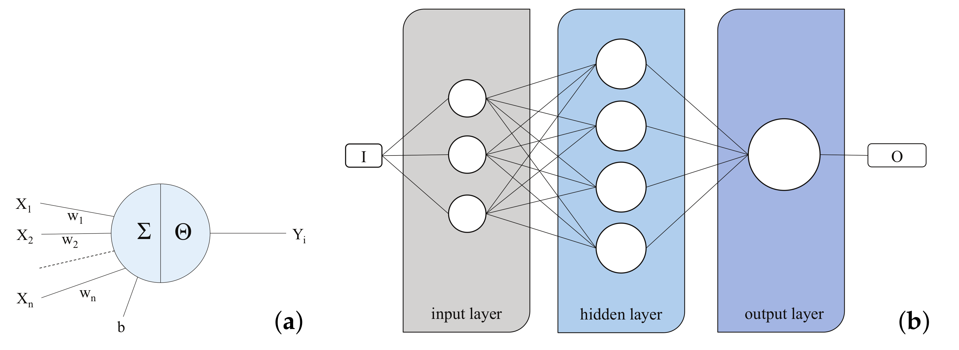
An artificial neural network is a general term encompassing many different architectures. Based on the literature mentioned in the introduction, a feed-forward neural network (FNN) might offer a suitable architecture to attain the stated objective of predicting the total volume of sediment flushed. A FNN are the simplest ANN structure, as the connections between the nodes of the network do not form a cycle and information passes straight (i.e., forward) through the network. The nodes (or neurons) of the ANN are processing units of the information, passing straight forward through the net. The nodes can be mathematically be formulated as follows:
where is the input information of the neuron, the synaptic weight, is the response characteristic (or transfer function) of the neuron, and Y is the output vector. Figure 1a shows such an artificial neuron schematically. In theory, a neuron can have multiple inputs and a single output. In addition to the external input , a bias b is added, in order to improve the convergence of the network. An ANN consists of the three main components—the input layer, one or more hidden layers, and the output layer—each consisting of a certain number of neurons. Figure 1b shows an example of an ANN, consisting of three layers: The input layer, a hidden layer with four neurons, and an output layer with one neuron. Depending on the problem, more complex architectures might be necessary. A comprehensive overview of the existing networks can be found in [30,31].
It is generally not clear how many layers are necessary for an ANN to understand a problem well. However, several studies have concluded that one hidden layer is optimal for most river-engineering problems, which is therefore applied in the following [32,33,34].
The neurons of the hidden and output layer are mapped using a transfer function (TF). This function transfers the input from an unlimited range to an output of a certain range. Different transfer functions have been described in the literature [27,30,31,32,35]. The most suitable TF for the hidden layer was estimated by an iterative trial-and-error approach. However, based on the evidence from previous research [14], it was decided to apply the unbound linear TF for the output layer, in order not to limit the output to a certain range, which is recommended for function fitting or non-linear regression problems. Table 1 shows the investigated combinations, using the abbreviations according to Matlab conventions. Here, “purelin” stands for the linear transfer function, which transfers an input (n) to an output (a) by . Furthermore, “logsig” is the log-sigmoid transfer function, which squashes the input into by . “Tansig” represents the hyperbolic tangent sigmoid transfer function, whose output is in the range from using . The abbreviation for the radial basis transfer function is “radbas” with . The transfer function “poslin” returns the output n if n is greater than or equal to zero and 0 if n is less than or equal to zero. “Satlin” is the saturated linear transfer function using if , if , or if , such that the output is in the range . Similar to satlin is “satlins”, which is a symmetric saturating linear transfer function using if , if , or if . An extension to radbas is “radbasn”, which is the normalized radial basis trasfer function using . Finally, "tribas" represents a triangular basis transfer function using if , and otherwise.
In addition, the most suitable number of neurons in the hidden layer of the ANN cannot be pre-defined. However, we can estimate a feasible range of neurons using the following Equation [14,36]:
where and represent the number of input and output nodes, respectively. The number of neurons is very important, as too small a number can lead to underfitting of the network, while too large a number can cause overfitting and unnecessarily high computational effort.
Initially, the weights of the network are randomly defined. In the training procedure, the weights and biases of the network are adjusted, such that the output of the network matches a given target. For this procedure, the Levenberg–Marquardt learning algorithm was used, which has shown good performance in other river-engineering applications [28,32,35]. Note that, in this study, Matlab (Version 2020a) was used to design and train the network.
2.2. Study Site
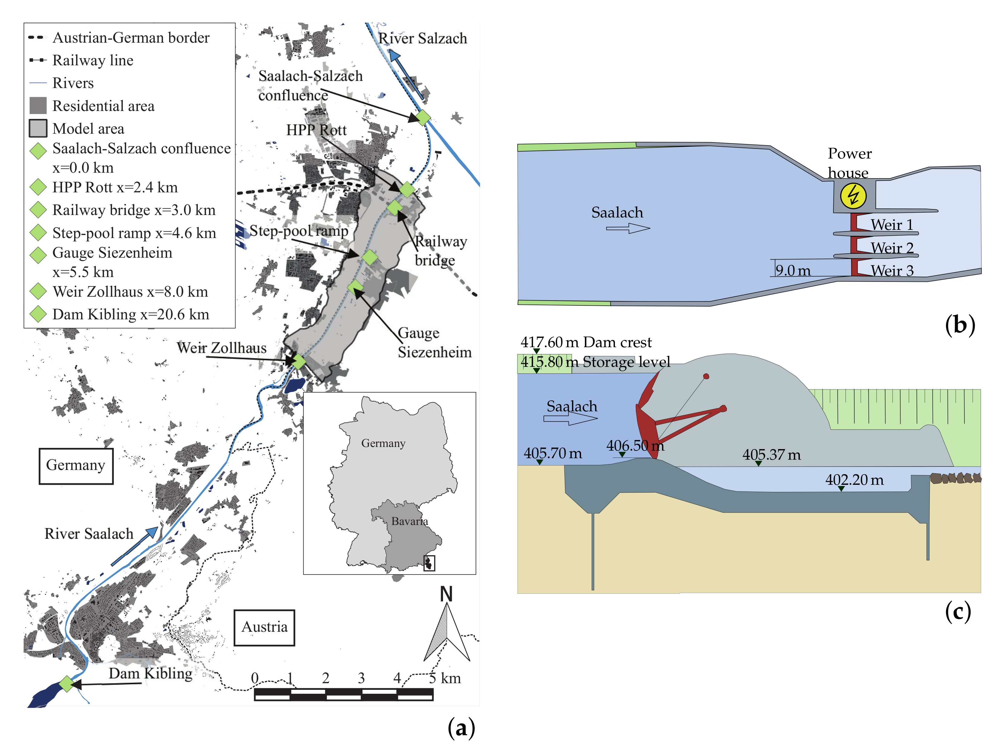
The study site for this research was a lower section of the alpine Saalach River at the German–Austrian border. Figure 2a provides an overview of the study site, highlighting important points along the river. The run-of-river HPP Rott dams the river to produce energy and, as originally intended, to stabilize the riverbed (Co-ordinates: Lat, 47.835047; Long, 12.994155). Figure 2b,c show schematic sketches of the HPP. The lower Saalach river transports a huge amount of coarse sediment (e.g., around m3/year are supplied into the river downstream of the Dam Kibling on average), which would accumulate in the reservoir of the HPP Rott if no sediment management were performed. However, the operator has to guarantee that the riverbed in the reservoir does not exceed a defined riverbed level. Therefore, drawdown flushing of the reservoir is irregularly performed, induced by opening of the weirs (three in total), thus lowering the water level. During normal operations of the HPP, the water level in the reservoir is equal to the storage level of m (Figure 2c). It deviates from this level only during higher flood events or when flushing [9].
The applicability and accuracy of the ANN developed herein depends heavily on the data available to train the network. The data have to reflect a wide range of possible situations, as ANNs are good for interpolation, but less suited for extrapolation to data outside of the training range. At this HPP, only sparse documentation on flushing, consisting of six real flushing events, was available for this study. This database was too small for our purpose.
Therefore, an already existing two-dimensional hydromorphological numerical model of this section, based on the TELEMAC-SISYPHE modeling system, was used as a surrogate to generate a larger data set for training the ANN. In the numerical model, the two-dimensional flow module TELEMAC2D was coupled with the sediment module SISYPHE. The model was initially designed to simulate the long-term morphological development of this river section under different hydropower operational schemes and reaches; therefore, from the gauge at Sizenheim to the HPP Rott (Figure 2a). The details of this numerical model have been reported in other publications [9,37]. Table 2 summarizes, therefore, just the main model parameters.
As mentioned above, this hydomorphological model was used to synthetically generate a broader, but still realistic database. For the numerical simulations, the discharge time-series from 1 January 2006 to 31 December 2013, measured at the gauge Siezenheim, was applied as the inflow boundary condition. In order to obtain a sufficiently large and heterogeneous database for training the network, different flushing scenarios (numbered with the index i) were generated. Therefore, for each scenario, a different threshold discharge Qf,i was defined, meaning that flushing is performed when this value is exceeded. In total, nine scenarios with the corresponding threshold discharges were developed: Qf,i = [100, 125, 150, 175, 200, 225, 250, 275, 300] [m/s]. Applying these values to the eight year-long discharge time-series, the corresponding water surface level at the HPP was defined for each scenario, denoted as Zf,i [m] in the following.
Figure 3 shows one exemplary flushing operation from of the eight years. Here, the differences between the generated scenarios are shown for a specific flow situation, which is around an HQ2 discharge. It can be seen that the lowering of the water level from the storage level ZS = 415.80 m started differently in each scenario, depending on the specific threshold discharge Qf,i. The lowering continued until free-flowing conditions were reached. When the discharge decreased and fell below the threshold, the water level increased again until ZS was reached. The gradient for lowering and raising of the water level was defined, for this HPP, at 0.5 m/h. This depended mainly on the stability of the embankments of the reservoir.
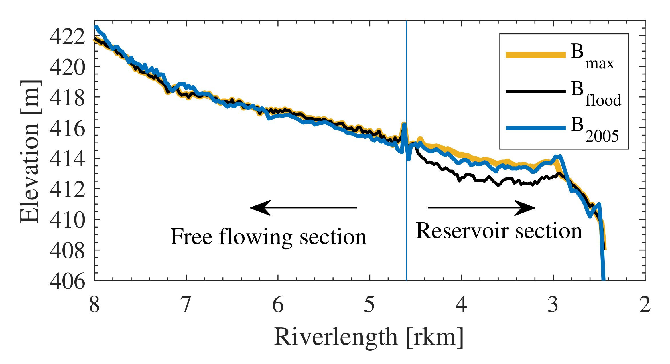
Furthermore, we expect that the volume of sediment in the domain (or the riverbed elevation) prior to a specific flushing operation makes a difference to the flushing efficiency. Thus, three different initial bathymetries for the 2D numerical model were also defined: The first representing the highest observed riverbed (Bmax), the second was the design riverbed for flood protection (Bflood), and the third was the riverbed measured in 2005/6 (B2005). Figure 4 shows the differences, by means of a longitudinal plot of the mean riverbed of the 2D model along the domain. It can be seen that Bmax had the highest elevation, especially in the reservoir section downstream from 4.6 km. Bflood was, in comparison, clearly lower, as it was designed to reduce inundation in the case of flood events [37]. In the free-flowing section, both bathymetries were the same, as the inundation was not critical. The third bathymetry B2005 was similar to Bmax, but was lower in the reservoir section and had some alterations in the free flowing section. With these defined initial and boundary conditions, a total of 27 (9 flushing scenarios × 3 inital bathymetries) numerical 2D simulations for the time period of eight years were carried out (Table 3).
2.3. Data Preparation
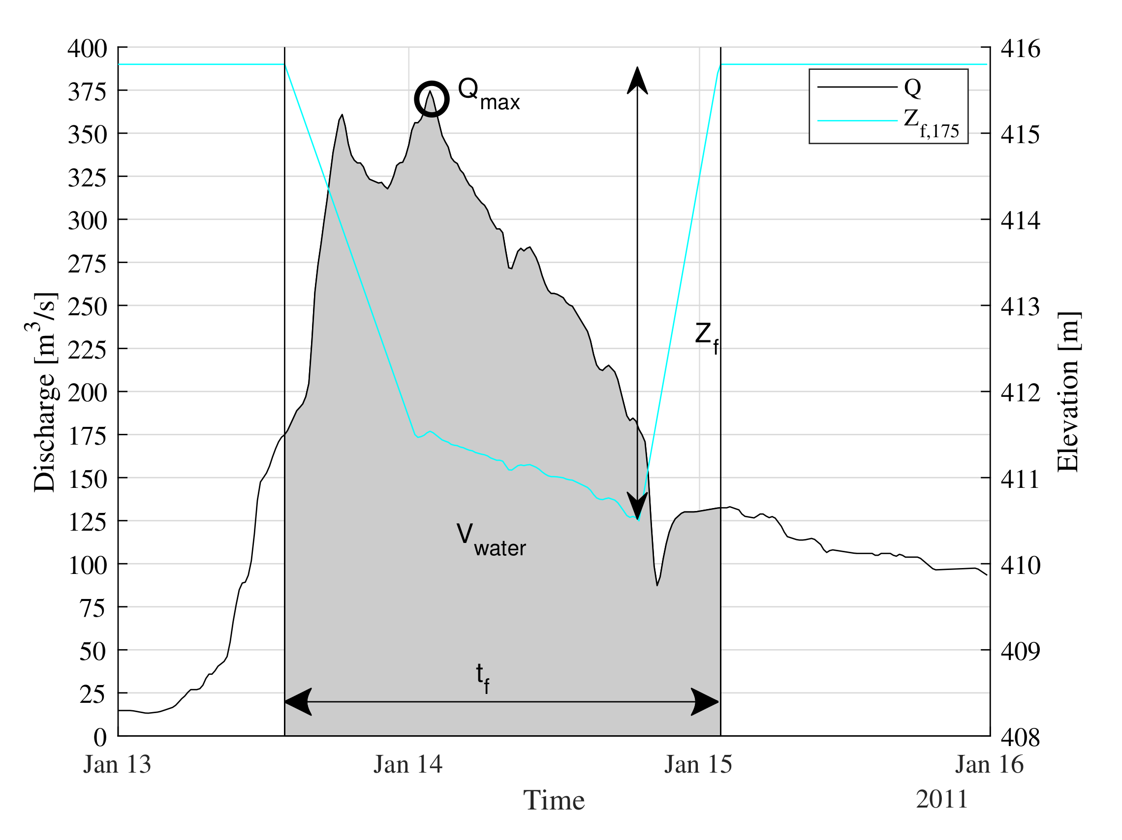
From these 27 initially conducted numerical simulations, each covering a period of eight years, around 600 different single flushing events were extracted. Figure 5 shows one exemplary flushing event, including the time-series of the discharge and the water elevation at the HPP. It should be noted that a single flushing event was defined from the time when the inflow discharge exceeded the threshold discharge and lasted until the discharge fell below this value, which happened frequently over the simulated time. However, such a flushing event consists of continuous temporal data (e.g., Q(t) or Zf(t)), which means that the data needed to be further processed and prepared in a suitable way.
The ANN applied required discrete input and target data. According to the literature and our expectations, the amount of sediment flushed depends on the flow present, the operation of the weir, and the initial riverbed before flushing [9]. However, it was not clear how to derive these input parameters from the continuous time-series data of the numerical simulation. Therefore, we defined different parameters to describe a single flushing event, which served later as input to the ANN: The first parameter we defined was the peak discharge during the flushing event, Qmax. This parameter alone might not be sufficient to distinguish different flow situations (e.g., a narrow but steep flow curve and a broad wave shape with same peak discharge). Furthermore, for a case like that shown in Figure 5, where two peaks are present, the peak discharge by itself might not be enough. Therefore, a second parameter, the total volume of water passing the weir during flushing, Vwater, was defined. Furthermore, the operation of the weir must be considered. Here, we defined the duration of flushing, tf, and the minimum water level reached during flushing, Zf,min. The fifth parameter noted was the initial volume of sediment in the domain before flushing, Vb,initial. However, as Vb,initial is hard to estimate in reality, a normalized variable is introduced here instead. The new parameter was defined as LoA = , denoting the level of aggregation before a flushing event. At this study site, a maximum acceptable riverbed in the reservoir has been defined by the authorities. The volume of this riverbed was calculated as Vb,max, corresponding to the volume of the initial bathymetry Bmax. The lowest riverbed of all simulations was used to estimate the minimum volume, Vb,min. This enabled the real use of such a network, as the LoA ratio can also be estimated in reality.
Finally, the target (and, thus, output) value of the ANN was the total volume of sediment, Vf, leaving the domain during flushing. This information was obtained by temporal integration of the sediment flux leaving the domain at the outlet, which are the weirs of the HPP.
2.4. Training Methodology
In the section above, we described possible input parameters for the ANN, which were proposed according to our expertise. However, in order to optimize the network architecture and to see their influence on the output, combinations of the described parameters were tested through a training procedure, as highlighted in Table 4.
Furthermore, for training the network, input and target values were each normalized into the range , using their min–max values after the following equation:
The corresponding min and max values are provided in Table 5.
The variability and heterogeneity of the input and target values are shown in Figure 6 using boxplots, in which the median and the 25% quantiles are highlighted. As mentioned above, a high variability is necessary to obtain a general and applicable ANN.
During the training step, the ANN learns the relationship between the input and target data. Before training, the prepared data are first separated randomly into three subsets—training (70%), testing (15%), and validation (15%)—to avoid overfitting and to obtain a generally applicable ANN. Moreover, the number of neurons was tested iteratively, from 2 to 11, using Equation (2). It is important to mention that the initial weights can also have a major impact on the possible accuracy of a network. In order to avoid this effect, training was conducted several times with new initial weights. In this study, the number of runs for each combination of a number of neurons in the hidden layer (10) and each IP Combination (5), as well as for the TF Combination (9), was 500.
Furthermore, the reliability and performance of the best network developed was investigated further, through a sensitivity analysis. In this analysis, a selected input parameter was changed in a certain bandwidth by multiplication with a factor fs, following the equation:
where X is the initial input and Xs is the modified input parameter. This indicates whether the ANN can also deal with data outside of the training range.
2.5. Performance Criteria
The correlation coefficient (R, Equation (5)), as a relative error measure, and the Root Mean Square Error (RMSE, Equation (6)) and the Mean Absolute Error (MAE, Equation (7)), as absolute error measures, were selected to investigate and evaluate the performance of the different trained networks:
where n is the number of data pairs, and and are the ith predicted and measured values, respectively.
3. Results
3.1. Training
The previously explained training procedure was carried out by testing the number of neurons and the different transfer functions. In total, 225,000 different networks were obtained, which were then analyzed, as detailed in the following. Note that the error criteria to evaluate the performance of the ANNs were evaluated by calculating the error measure from the test sub set. Figure 7 shows the categorized overview of the performance of the different ANNs using boxplots: (a) The transfer function combination; (b) the number of neurons; and (c) the input parameter combination.
It is evident that the TF Combinations 9 (purelin–purelin) and 4 (poslin–purelin) clearly had the worst performance, indicating that a TF based on a linear function in the hidden layer is not optimal. Moreover, other TFs with linear functions (5, 6, and 8) in the hidden layer were only slightly better. Indeed, non-linear TFs 1–3 and 7 showed similar accuracy and the lowest RMSEs. The differences in their performance were negligible and similar results could be obtained (Figure 7a). Furthermore, it is evident that, with an increasing number of neurons, the accuracy of all networks increased independently of the TF, but stopped at nine neurons (Figure 7b). This means that a higher number of neurons would lead to results of the same accuracy, but requires additional computational power with no further advantage. Figure 7c shows that the accuracy of the networks increased with additional inputs and, as the same time, the bandwidth of the error became smaller. This means that the network architecture (TF, Number of Neurons) becomes less important and, in more cases, an accurate ANN could be obtained. It is clear that IPs 1 and 2 were the worst, which means that the other parameters were significant and must be considered. ANNs with IP options 3 and 5 obtained similar accuracy. However, it is evident that the input combination 4 was clearly the most accurate combination. This confirms that the LoA parameter is important for the ANN to understand the data. Moreover, adding the Vwater parameter clearly improved the performance.
The network which showed the best accuracy—that is, the network with the smallest difference (RMSE) between the measured data (Target) and the predicted ANN Output—was used for further tests. Of all 225,000 networks, the best ANN had TF-combination 2 (tansig–purelin), a number of neurons equal to 9, and IP-combination 4 (using all five parameters). Figure 8 shows the regression of the target data (x-axis) and the corresponding output of the ANN (y-axis) for all data (overall), and the subsets for training, validation, and testing, respectively. This illustrates very well that the ANN could learn the relationship between the inputs and the output, as the relation is almost linear. Moreover, the normalized RMSE of the ANN was very low and close to zero. In order to give the absolute error of the network a physical meaning, the values were de-normalized and the MAE was calculated. The best network had a MAE of 960 m3 for the test subset. This means that, on average, the ANN over- or under-predicts the volume of flushing, Vf, by this value; which is very low, considering possible flushing volumes of up to 100,000 m3.
3.2. Sensitivity
To validate whether the ANN works well as a general predictor of reservoir flushing, a sensitivity analysis on the input parameter LoA (the level of aggregation) was performed. This parameter represents the initial volume of sediment in the domain. It was expected that the higher this value was, the higher the amount of sediment flushed, and vice versa. Furthermore, this parameter was clearly independent of the others and could be analyzed alone, as it does not affect the flow present or the weir operation. For the sensitivity analysis, we multiplied this parameter with a factor fs = [0.7, 0.8, 0.9, 1.1, 1.2, 1.3], such that (Equation (4)), which is basically a decrease (fs < 1) or an increase (fs > 1) of the original LoA. These values, , were used in the sensitivity test as input for the previously determined ANN. The other parameters were kept unchanged.
Figure 9 shows the results of this analysis by means of scatter plots of the original results (ff = 1) against the output of the test. It is clear that increases of LoA by 10, 20, and 30%, respectively, (filled scatter points), led to an overall increase of the predicted output. This means a higher amount of sediment flushed, Vf. Correspondingly, the ANN predicted a lower output with a decreased LoA to 90, 80, and 70% (empty scatter points), respectively, as input. This closely followed our expectations and confirmed that the designed ANN has a basic understanding of the governing process. From a reservoir with a very low LoA—which means a very low riverbed—less sediment is mobilized during flushing than from a reservoir with a high riverbed closer to the water surface.
4. Discussion
The proposed tool, using data-driven methods for reservoir flushing estimation, showed promising results. The developed ANN identified a clear correlation between distinct input data and the desired mobilized sediment volume (i.e., the volume of sediment flushed). Although this approach is very simple, requiring only five simple inputs, the mean average error was so small that it can be neglected when the total uncertainty is considered. This was especially true in the case of the Saalach river, where we have, on average, high annual sediment loads of around 40,000 m3/year and, during one single flushing event, volumes as high as 20,000 or even 100,000 m3 are frequently mobilized.
One important point to discuss here is the origin of the training data: In order to develop an applicable and generally valid ANN, it is necessary to use a sufficiently large and heterogeneous database for training; that is, larger than the available data at this study site. Limited data was also one problem of a study using an ANN at the Three Gorges Dam; thus, the predictive ability of the model was not that good (e.g., ) [29]. To overcome this problem in our study, a sufficiently large amount of training data were obtained by using a numerical model as a surrogate for real measured data. The idea to use surrogate models in the absence of real data have also been applied in other studies, such as [33,34]. The numerical simulations in this study each covered a period of eight years and included several different flow conditions (e.g., flood events ranging from floods with a return period of 1 year up to 100 years), such that the ANN could learn a variety of possible situations. However, it must be highlighted that the network developed here is, therefore, only applicable to this particular river section. If the river system of the Saalach fundamentally changes in the future (e.g., due to the extension of the existing HPP by an additional gate or water extraction in the section between the discharge gauge and the HPP), the predictive ability of the ANN will decrease. In contrast, other changes in the system that affect the discharge regime will have no change. This could happen, for example, due to climate change, which could cause more frequent occurrence of extreme discharge events and longer periods of low water [39]. Here, the applicability of the ANN is not affected, as the frequency of flushing events or other temporal factors are not inputs of the designed ANN and each event is independent of the previous ones.
The overall concept underpinning this research is transferable to other study sites and extendable with additional parameters and inputs. If the described input data were gathered from different HPPs, a sufficiently large database consisting of real measurements could be obtained. If the data came from different HPPs, it might be necessary to include additional parameters representing the geometry (e.g., length and width) and granulometry (e.g., mean diameter dm) of the different reservoirs. Such a parameter was not necessary for this test, as the data were only obtained from the one site.
Moreover, in further research, the reservoir might be divided into several parts (e.g., lower and upper sections), in order to spatially locate where the volume is eroded. However, it might then be necessary to couple two ANNs together, each of which responsible for their own section.
Furthermore, it should be pointed out that it took around 87 h per simulation (8 years in reality) and, so, 2349 h in total to generate the database for training. This is a heavy time load, although the Cool-MUC-2 HPC system of the Leibniz Computing Center was used and the 2D numerical modeling software TELEMAC-SISYPHE can run efficiently in parallel mode using domain decomposition techniques [40]. This clearly highlights the huge computational effort which is necessary to investigate sediment flushing by numerical methods. Of course, this effort was also necessary to obtain the database used in the present study, but the trained ANN needed only 1 second on a standard computer to evaluate the volume of flushing for the 600 different scenarios.
The performed sensitivity analysis of our study case confirmed that the ANN determined a general relationship between the input and target data. By changing the initial volume of sediment in the domain before the flushing (LoA), the predicted output behaved according to our expectations. In further work, the sensitivity of other parameters could also be investigated. However, it should then be remembered that these parameters can influence each other. An increasing peak discharge affects the volume of the water, as well as the free-flowing water level during flushing. Moreover, with a change of peak discharge, the duration of the flushing will also change. Therefore, sensitivity analyses were only performed on the LoA herein, as this value is independent of the others.
It must be mentioned that an ANN is just one data-driven approach for the detection of non-linear correlations. Many other different methods are available. In particular, support vector machine (SVM) models may provide a suitable alternative. This approach has been successfully applied to reconstruct streamflows from different data types [41] or for the prediction of suspended sediment loads (SSL) [42]. Some studies have compared the performance of both approaches (i.e., ANN and SVM) and obtained similar accuracy with both models, for example, to model soil pollution [43] or to predict the monthly river flow [44]. Moreover, stochastic modeling (SM) by the multivariate regression method could also be an option worth mentioning [45,46]. In a further study, one could evaluate how SVM and SM models perform for the purpose of reservoir flushing, compared to the ANN concept presented here.
Finally, the developed ANN is transferable in a simple, executable GUI, which can run on every computational system. It can be easily integrated into the operation and management procedure of any reservoir. Figure 10 shows a sketch of a possible workflow. Given the near-future hydrograph (e.g., from a hydrological model), the input Qmax, the peak discharge of the expected flood wave can be defined. Further, required inputs can be defined or calculated, such as the volume of the hydrograph Vwater, the duration of the flushing tf, and the minimum water level reached Zf,min, such that the ANN can predict the volume of sediment flushed from the reservoir given this specific operation. If the volume is considered as effective in lowering the riverbed (decision = yes), the flushing can be initiated. If not (decision = no), another operation mode (e.g., an increased tf, which means a longer flushing operation) can be tested; or, if no operation leads to a desired high volumetric output, the flushing can be postponed until a bigger discharge is estimated.
5. Conclusions
The main conclusions of this research can be summarized as follows:
- In general, artificial neural networks (ANN) are powerful additional tools for river management.
- A feed-forward neural network can accurately predict the volume of sediment flushed during a single event, based on discrete input parameters.
- The developed ANN can be embedded into existing management structures, providing a decision-support system for reservoir operators.
- Extension of the approach to other study areas and, thus, the inclusion of more data are highly recommended.
Author Contributions
Conceptualization, M.R. and M.D.B.; methodology, M.R.; software, M.R.; validation, M.R., M.D.B. and P.R.; formal analysis, M.R.; investigation, M.R.; resources, M.R.; data curation, M.R.; writing–original draft preparation, M.R.; writing–review and editing, M.R. and M.D.B.; visualization, M.R.; supervision, P.R. All authors have read and agreed to the published version of the manuscript.
Funding
This research received no external funding.
Institutional Review Board Statement
Not applicable.
Informed Consent Statement
Not applicable.
Data Availability Statement
The data presented in this study are available on request from the corresponding author.
Acknowledgments
The authors thank the Leibnitz Computing Centre (LRZ, Garching near Munich) for the HPC system to conduct the numerical simulations.
Conflicts of Interest
The authors declare no conflict of interest.
References
- Habersack, H.; Hein, T.; Stanica, A.; Liska, I.; Mair, R.; Jäger, E.; Hauer, C.; Bradley, C. Challenges of river basin management: Current status of, and prospects for, the River Danube from a river engineering perspective. Sci. Total Environ. 2016, 543, 828–845. [Google Scholar] [CrossRef] [PubMed] [Green Version]
- Schleiss, A.J.; Franca, M.J.; Juez, C.; De Cesare, G. Reservoir sedimentation. J. Hydraul. Res. 2016, 54, 595–614. [Google Scholar] [CrossRef]
- Guillén-Ludeña, S.; Manso, P.; Schleiss, A. Multidecadal Sediment Balance Modelling of a Cascade of Alpine Reservoirs and Perspectives Based on Climate Warming. Water 2018, 10, 1759. [Google Scholar] [CrossRef] [Green Version]
- Ludeña, S.G.; Manso, P.; Schleiss, A.J.; Schwegler, B.; Stamm, J.; Fankhauser, A. Sediment balance of a cascade of alpine reservoirs based on multi-decadal data records. E3S Web Conf. 2018, 40, 03012. [Google Scholar] [CrossRef] [Green Version]
- Annandale, G.W.; Morris, G.L.; Karki, P. Extending the Life of Reservoirs: Sustainable Sediment Management for Dams and Run-of-River Hydropower; World Bank Group: Washington, DC, USA, 2016; Available online: http://documents.worldbank.org/curated/en/794841476187802040/Extending-the-life-of-reservoirs-sustainable-sediment-management-for-dams-and-run-of-river-hydropower (accessed on 1 October 2020).
- Reckendorfer, W.; Badura, H.; Schütz, C. Drawdown flushing in a chain of reservoirs—Effects on grayling populations and implications for sediment management. Ecol. Evol. 2019, 9, 1437–1451. [Google Scholar] [CrossRef] [Green Version]
- Isaac, N.; Eldho, T.I. Sediment management studies of a run-of-the-river hydroelectric project using numerical and physical model simulations. Int. J. River Basin Manag. 2016, 14, 165–175. [Google Scholar] [CrossRef]
- Isaac, N.; Eldho, T.I. Sediment removal from run-of-the-river hydropower reservoirs by hydraulic flushing. Int. J. River Basin Manag. 2019, 1–14. [Google Scholar] [CrossRef]
- Reisenbüchler, M.; Bui, M.D.; Skublics, D.; Rutschmann, P. Sediment Management at Run-of-River Reservoirs Using Numerical Modelling. Water 2020, 12, 249. [Google Scholar] [CrossRef] [Green Version]
- Bui, M.D.; Rutschmann, P. Numerical modelling for reservoir sediment management. In Proceedings of the ASIA 2016, Sixth International Conference and Exhibition on Water Resources and Hydropower Development in Asia, Vientiane, Laos, 1–3 March 2016. [Google Scholar]
- Chaudhary, H.P.; Isaac, N.; Tayade, S.B.; Bhosekar, V.V. Integrated 1D and 2D numerical model simulations for flushing of sediment from reservoirs. ISH J. Hydraul. Eng. 2019, 25, 19–27. [Google Scholar] [CrossRef]
- Dépret, T.; Piégay, H.; Dugué, V.; Vaudor, L.; Faure, J.B.; Le Coz, J.; Camenen, B. Estimating and restoring bedload transport through a run-of-river reservoir. Sci. Total Environ. 2019, 654, 1146–1157. [Google Scholar] [CrossRef]
- Gallerano, F.; Cannata, G. Compatibility of Reservoir Sediment Flushing and River Protection. J. Hydraul. Eng. 2011, 137, 1111–1125. [Google Scholar] [CrossRef]
- Ateeq-Ur-Rehman, S. Numerical Modeling of Sediment Transport in Dasu-Tarbela Reservoir using Neural Networks and TELEMAC Model System; Technische Universität München: München, Germany, 2019; Available online: http://mediatum.ub.tum.de/?id=1455875 (accessed on 1 October 2020).
- Esmaeili, T.; Sumi, T.; Kantoush, S.A.; Kubota, Y.; Haun, S.; Rüther, N. Three-Dimensional Numerical Study of Free-Flow Sediment Flushing to Increase the Flushing Efficiency: A Case-Study Reservoir in Japan. Water 2017, 9, 900. [Google Scholar] [CrossRef] [Green Version]
- Shields, A. Application of Similarity Principles and Turbulence Research to Bed-Load Movement; Hydrodynamics Laboratory California Institute of Technology: Pasadena, CA, USA, 1936; Volume 167, Available online: https://authors.library.caltech.edu/25992/1/Sheilds.pdf (accessed on 1 October 2020).
- Wu, W. Depth-Averaged Two-Dimensional Numerical Modeling of Unsteady Flow and Nonuniform Sediment Transport in Open Channels. J. Hydraul. Eng. 2004, 130, 1013–1024. [Google Scholar] [CrossRef]
- Juez, C.; Murillo, J.; García-Navarro, P. Numerical assessment of bed-load discharge formulations for transient flow in 1D and 2D situations. J. Hydroinform. 2013, 15, 1234–1257. [Google Scholar] [CrossRef]
- Sindelar, C.; Gold, T.; Reiterer, K.; Hauer, C.; Habersack, H. Experimental Study at the Reservoir Head of Run-of-River Hydropower Plants in Gravel Bed Rivers. Part I: Delta Formation at Operation Level. Water 2020, 12, 2035. [Google Scholar] [CrossRef]
- Reiterer, K.; Gold, T.; Habersack, H.; Hauer, C.; Sindelar, C. Experimental Study at the Reservoir Head of Run-of-River Hydropower Plants in Gravel Bed Rivers. Part II: Effects of Reservoir Flushing on Delta Degradation. Water 2020, 12, 3038. [Google Scholar] [CrossRef]
- Bieri, M.; Müller, M.; Boillat, J.L.; Schleiss, A.J. Modeling of Sediment Management for the Lavey Run-of-River HPP in Switzerland. J. Hydraul. Eng. 2012, 138, 340–347. [Google Scholar] [CrossRef]
- El Bilali, A.; Taleb, A.; El Idrissi, B.; Brouziyne, Y.; Mazigh, N. Comparison of a data-based model and a soil erosion model coupled with multiple linear regression for the prediction of reservoir sedimentation in a semi-arid environment. Euro-Mediterr. J. Environ. Integr. 2020, 5, 64. [Google Scholar] [CrossRef]
- Garg, V.; Jothiprakash, V. Evaluation of reservoir sedimentation using data driven techniques. Appl. Soft Comput. 2013, 13, 3567–3581. [Google Scholar] [CrossRef]
- Jothiprakash, V.; Garg, V. Reservoir Sedimentation Estimation Using Artificial Neural Network. J. Hydrol. Eng. 2009, 2009. 14, 1035–1040. [Google Scholar] [CrossRef]
- Apaydin, H.; Feizi, H.; Sattari, M.T.; Colak, M.S.; Shamshirband, S.; Chau, K.W. Comparative Analysis of Recurrent Neural Network Architectures for Reservoir Inflow Forecasting. Water 2020, 12, 1500. [Google Scholar] [CrossRef]
- Ateeq-Ur-Rehman, S.; Bui, M.; Rutschmann, P. Variability and Trend Detection in the Sediment Load of the Upper Indus River. Water 2018, 10, 16. [Google Scholar] [CrossRef] [Green Version]
- Tarar, Z.R.; Ahmad, S.R.; Ahmad, I.; Hasson, S.u.; Khan, Z.M.; Washakh, R.M.A.; Ateeq-Ur-Rehman, S.; Bui, M.D. Effect of Sediment Load Boundary Conditions in Predicting Sediment Delta of Tarbela Reservoir in Pakistan. Water 2019, 11, 1716. [Google Scholar] [CrossRef] [Green Version]
- Bui, M.D.; Kaveh, K.; Penz, P.; Rutschmann, P. Contraction scour estimation using data-driven methods. J. Appl. Water Eng. Res. 2015, 3, 143–156. [Google Scholar] [CrossRef]
- Li, X.; Qiu, J.; Shang, Q.; Li, F. Simulation of Reservoir Sediment Flushing of the Three Gorges Reservoir Using an Artificial Neural Network. Appl. Sci. 2016, 6, 148. [Google Scholar] [CrossRef] [Green Version]
- Haykin, S.S. Neural Networks: A Comprehensive Foundation: Solutions Manual; Macmillan College Publishing Company: New York, NY, USA, 1994. [Google Scholar]
- Haykin, S.; Haykin, S. Neural Networks and Learning Machines; Pearson Education, Inc.: Upper Saddle River, NJ, USA, 2009. [Google Scholar]
- Ateeq-Ur-Rehman, S.; Bui, M.D.; Hasson, S.U.; Rutschmann, P. An Innovative Approach to Minimizing Uncertainty in Sediment Load Boundary Conditions for Modelling Sedimentation in Reservoirs. Water 2018, 10, 1411. [Google Scholar] [CrossRef] [Green Version]
- Bui, V.H.; Bui, M.D.; Rutschmann, P. The Prediction of Fine Sediment Distribution in Gravel-Bed Rivers Using a Combination of DEM and FNN. Water 2020, 12, 1515. [Google Scholar] [CrossRef]
- Bui, V.H.; Bui, M.D.; Rutschmann, P. Combination of Discrete Element Method and Artificial Neural Network for Predicting Porosity of Gravel-Bed River. Water 2019, 11, 1461. [Google Scholar] [CrossRef] [Green Version]
- Kaveh, K.; Bui, M.D.; Rutschmann, P. A new approach for morphodynamic modeling using integrating ensembles of artificial neural networks. In Wasserbau—Mehr als Bauen im Wasser, Proceedings of the 18th Symposium of TU Munich, TU Graz and ETH Zurich, TU Graz, Austria, 11–14 September 2019; Huber, R., Ed.; Rutschmann, Peter: London, UK, 2019; Volume 134, pp. 304–315. Available online: https://www.bgu.tum.de/fileadmin/w00blj/wb/Publikationen/Berichtshefte/Band134.pdf (accessed on 1 October 2020).
- Shahin, M.A.; Maier, H.R.; Jaksa, M.B. Predicting Settlement of Shallow Foundations using Neural Networks. J. Geotech. Geoenviron. Eng. 2002, 128, 785–793. [Google Scholar] [CrossRef]
- Reisenbüchler, M.; Bui, M.D.; Skublics, D.; Rutschmann, P. Enhancement of a numerical model system for reliably predicting morphological development in the Saalach River. Int. J. River Basin Manag. 2020, 18, 335–347. [Google Scholar] [CrossRef]
- Hunziker, R.P. Fraktionsweiser Geschiebetransport; Laboratory of Hydraulics, Hydrology and Glaciology (VAW), ETH Zürich: Zürich, Switzerland, 1995; Volume 11037, p. 191. [Google Scholar] [CrossRef]
- Goler, R.A.; Frey, S.; Formayer, H.; Holzmann, H. Influence of Climate Change on River Discharge in Austria. Meteorol. Z. 2016, 25, 621–626. [Google Scholar] [CrossRef]
- Moulinec, C.; Denis, C.; Pham, C.T.; Rougé, D.; Hervouet, J.M.; Razafindrakoto, E.; Barber, R.W.; Emerson, D.R.; Gu, X.J. TELEMAC: An efficient hydrodynamics suite for massively parallel architectures. Comput. Fluids 2011, 51, 30–34. [Google Scholar] [CrossRef] [Green Version]
- Chiogna, G.; Marcolini, G.; Liu, W.; Pérez Ciria, T.; Tuo, Y. Coupling hydrological modeling and support vector regression to model hydropeaking in alpine catchments. Sci. Total Environ. 2018, 633, 220–229. [Google Scholar] [CrossRef]
- Nourani, V.; Alizadeh, F.; Roushangar, K. Evaluation of a Two-Stage SVM and Spatial Statistics Methods for Modeling Monthly River Suspended Sediment Load. Water Resour. Manag. 2016, 30, 393–407. [Google Scholar] [CrossRef]
- Sakizadeh, M.; Mirzaei, R.; Ghorbani, H. Support vector machine and artificial neural network to model soil pollution: A case study in Semnan Province, Iran. Neural Comput. Appl. 2017, 28, 3229–3238. [Google Scholar] [CrossRef]
- Ghorbani, M.A.; Zadeh, H.; Isazadeh, M.; Terzi, O. A comparative study of artificial neural network (MLP, RBF) and support vector machine models for river flow prediction. Environ. Earth Sci. 2016, 75. [Google Scholar] [CrossRef]
- Bishop, P.L.; Hively, W.D.; Stedinger, J.R.; Rafferty, M.R.; Lojpersberger, J.L.; Bloomfield, J.A. Multivariate analysis of paired watershed data to evaluate agricultural best management practice effects on stream water phosphorus. J. Environ. Qual. 2005, 34, 1087–1101. [Google Scholar] [CrossRef] [PubMed]
- Le, T.M.K.; Mäkelä, M.; Schreithofer, N.; Dahl, O. A multivariate approach for evaluation and monitoring of water quality in mining and minerals processing industry. Miner. Eng. 2020, 157, 106582. [Google Scholar] [CrossRef]
Figure 1.
(a) Scheme of an artificial neuron; and (b) Scheme of a Feed-forward network.

Figure 2.
(a) Overview of the study site, including the extent of the numerical model and the important sites along the river [37]; and sketches of the HPP Rott in top (b) and longitudinal sectional (c) views [9].

Figure 3.
Time-series of the flow (Q) and the nine different developed scenarios, represented by the water surface elevation (Zf,i) for one exemplary flow situation.
Figure 3.
Time-series of the flow (Q) and the nine different developed scenarios, represented by the water surface elevation (Zf,i) for one exemplary flow situation.

Figure 4.
Longitudinal section of the mean river bed for the three different initial bathymetries B.
Figure 4.
Longitudinal section of the mean river bed for the three different initial bathymetries B.

Figure 5.
Discretisation of continuous time-series of the hydrograph (Q) and water surface elevation (Zf) into five parameters, exemplary for one event of scenario Zf,175.
Figure 5.
Discretisation of continuous time-series of the hydrograph (Q) and water surface elevation (Zf) into five parameters, exemplary for one event of scenario Zf,175.

Figure 6.
Analysis of the five input parameters and the output parameter.

Figure 7.
Influence on the performance of the ANNs by: (a) The transfer function (TF); (b) the number of neurons; and (c) the input parameter (IP) combination.
Figure 7.
Influence on the performance of the ANNs by: (a) The transfer function (TF); (b) the number of neurons; and (c) the input parameter (IP) combination.

Figure 8.
Regression of the original data (Target) and the predicted data (Output) for all data (overall), and for each of the training, validation, and testing subsets.
Figure 8.
Regression of the original data (Target) and the predicted data (Output) for all data (overall), and for each of the training, validation, and testing subsets.

Figure 9.
Scatter plot of the original ANN output (fs = 1; x-axis) against the test output (y-axis) with decreasing/increasing (fs = [0.7, 0.8, 0.9, 1.0, 1.1, 1.2, 1.3]) as input.
Figure 9.
Scatter plot of the original ANN output (fs = 1; x-axis) against the test output (y-axis) with decreasing/increasing (fs = [0.7, 0.8, 0.9, 1.0, 1.1, 1.2, 1.3]) as input.

Figure 10.
Integration of the developed ANN as a decision support tool for reservoir management.


Table 1.
Different tested combinations of transfer functions (TFs) for the hidden and output layers.
Table 1.
Different tested combinations of transfer functions (TFs) for the hidden and output layers.
| # | Hidden–Output |
|---|---|
| 1 | logsig–purelin |
| 2 | tansig–purelin |
| 3 | radbas–purelin |
| 4 | poslin–purelin |
| 5 | satlin–purelin |
| 6 | satlins–purelin |
| 7 | radbasn–purelin |
| 8 | tribas–purelin |
| 9 | purelin–purelin |
Table 2.
Main model parameters of the 2D hydromorphological model.
| Parameter | Value |
|---|---|
| Riverbed roughness (Strickler) kst | 35 m/s |
| Form roughness (Strickler) kst,r | Sectional calibrated [22–35] m/s |
| Bedload transport formula | Hunziker [38] |
| Shields-parameter | 0.04 (for all grain classes) |
| Active layer thickness | 0.14 m = dmax |
| Number of grain classes | 8 |
| Mean diameter of the single grain classes [mm] | 0.5, 2, 8, 16, 31.5, 60, 93, 140 |
Table 3.
Overview of the numerical configurations to obtain the database.
| Initial Batyhmetry Bi | Threshold Discharge Qf,i [m3/s] | ||||||||||
|---|---|---|---|---|---|---|---|---|---|---|---|
| max | 2005 | flood | 100 | 125 | 150 | 175 | 200 | 225 | 250 | 275 | 300 |
Table 4.
Different combinations of input parameters (IPs).
| # | Input Parameters |
|---|---|
| 1 | Qmax, Zf,min |
| 2 | Qmax, Zf,min, tf |
| 3 | Qmax, Zf,min, tf, Vwater |
| 4 | Qmax, Zf,min, tf, Vwater, LoA |
| 5 | Qmax, Zf,min, tf, LoA |
Table 5.
Range of the Input and Target used for normalization.
| Qmax | Vwater | tf | Zf,min | LoA | Vf | |
|---|---|---|---|---|---|---|
| [m3/s] | [m3] | [h] | [m] | [/] | [m3] | |
| Min | 100.08 | 2.623·105 | 0.5 | 409.695 | 0.2037 | 5.479·10−5 |
| Max | 1.083·103 | 1.900·108 | 379 | 415.7 | 1.293 | 1.003·105 |
Publisher’s Note: MDPI stays neutral with regard to jurisdictional claims in published maps and institutional affiliations. |
© 2021 by the authors. Licensee MDPI, Basel, Switzerland. This article is an open access article distributed under the terms and conditions of the Creative Commons Attribution (CC BY) license (http://creativecommons.org/licenses/by/4.0/).
Share and Cite
MDPI and ACS Style
Reisenbüchler, M.; Bui, M.D.; Rutschmann, P. Reservoir Sediment Management Using Artificial Neural Networks: A Case Study of the Lower Section of the Alpine Saalach River. Water 2021, 13, 818. https://doi.org/10.3390/w13060818
AMA Style
Reisenbüchler M, Bui MD, Rutschmann P. Reservoir Sediment Management Using Artificial Neural Networks: A Case Study of the Lower Section of the Alpine Saalach River. Water. 2021; 13(6):818. https://doi.org/10.3390/w13060818
Chicago/Turabian StyleReisenbüchler, Markus, Minh Duc Bui, and Peter Rutschmann. 2021. "Reservoir Sediment Management Using Artificial Neural Networks: A Case Study of the Lower Section of the Alpine Saalach River" Water 13, no. 6: 818. https://doi.org/10.3390/w13060818
Note that from the first issue of 2016, this journal uses article numbers instead of page numbers. See further details here.