
A Novel Method for Regional Short-Term Forecasting of Water Level


1
College of Geodesy and Geomatics, Shandong University of Science and Technology, Qingdao 266590, China
2
Shandong Electric Power Engineering Consulting Institute Corp., Ltd., Jinan 250013, China
3
Zhejiang Institute of Hydraulics & Estuary (Zhejiang Institute of Marine Planning and Design), Hangzhou 310020, China
4
Key Laboratory of Estuary and Coast of Zhejiang Province, Hangzhou 310020, China
5
Key Laboratory of Oceanic Surveying and Mapping, Ministry of Natural Resources of China, Qingdao 266590, China
6
Shanghai Institute of Optics and Fine Mechanics, Chinese Academy of Sciences, Shanghai 201800, China
*
Authors to whom correspondence should be addressed.
Water 2021, 13(6), 820; https://doi.org/10.3390/w13060820
Submission received: 11 December 2020
/
Revised: 11 March 2021
/
Accepted: 14 March 2021
/
Published: 17 March 2021
Abstract
:The water level forecasting system represented by the hydrodynamic model relies too much on the input data and the forecast value of the boundary, therefore introducing uncertainty in the prediction results. Tide tables ignore the effect of the residual water level, which is usually significant. Therefore, to solve this problem, a water level forecasting method for the regional short-term (3 h) is proposed in this study. First, a simplified MIKE21 flow model (FM) was established to construct the regional major astronomical tides after subdividing the model residuals into stationary constituents (surplus astronomical tides, simulation deviation) and nonstationary constituents (residual water level). Harmonic analysis (HA) and long short-term memory (LSTM) were adopted to forecast these model residuals, respectively. Finally, according to different spatial background information, the prediction for each composition was corrected by the inverse distance weighting (IDW) algorithm and its improved IDW interpolation algorithm based on signal energy and the spatial distance (IDWSE) from adjacent observation stations to nonmeasured locations. The developed method was applied to Narragansett Bay in Rhode Island. Compared with the assimilation model, the root-mean-square error (RMSE) of the proposed method decreased from 12.3 to 5.0 cm, and R2 increased from 0.932 to 0.988. The possibility of adding meteorological features into the LSTM network was further explored as an extension of the prediction of the residual water level. The results show that the accuracy was limited to a moderate level, which is related to the difficulty presented by using only wind features to completely characterize the regional dynamic energy equilibrium process.
1. Introduction
As one of the most widely used approaches for tidal prediction, the tide tables based on harmonic analysis (HA) [1] can accurately predict astronomical tides. However, tide tables cannot predict the residual water level caused by wind, barometric pressure, and discharge, which are quite significant. With the development of numerical simulation technology, the effect of environmental factors on water level changes has become a concern. As a result, a series of hydrodynamic models have been proposed [2,3]. Relying on a hydrodynamic model and the Physical Oceanographic Real-Time System (PORTS®) [4], the United States built a 48 h tidal forecast system in ports, estuaries, great lakes, and coastal waters [5,6,7], such as the Gulf of Maine Operational Forecast System (GOMOFS). In this system, the Regional Ocean Modeling System (ROMs) [8] is used as the core prediction model, and meteorological and hydrological prediction products are also assimilated. When evaluating the performance of GOMOFS, Peng et al. [9] found that the root-mean-square error (RMSE) between the prediction and the observation was larger than the RMSE between the observation and the astronomical tides prediction, indicating an unsatisfactory precision of prediction. The findings were the same in the Chesapeake Bay Operational Forecast System (CBOFS) [7].
Assimilation and correction of the Singapore regional model (SRM) [10] may be the work most similar to the research regional forecasting of water level. In these studies, prediction results from the model residuals are divided into two categories. One category is represented by chaos theory, in which the error is maintained at a medium level and does not change significantly [11]. For the second category, the error gradually diverges with lead time, such as in ensemble Kalman filters [12], neural networks [13], and other combined models [14]. Of note, as a product of numerical simulation, the forecast error always contains two tidal components [15]: The residuals of the simulated tides (simulation deviation) and the partial astronomical tides (surplus astronomical tides). The former is caused by the errors of bathymetry, coastline, parameters, open boundary, and so on, which will affect the total water depth and, in turn, affect the tide. The latter is caused by the number of tidal constituents at the open boundary, which are usually incomplete. For the prediction of nonstationary time series data, LSTM is considered to have excellent performance. Due to the dedicated “gate mechanism” [16], LSTM can remember variable lengths of time and has been successfully applied in the field of water level forecast, especially in marine disaster prevention (such as storm surges, floods) [17,18,19]. In fact, the short-time water level forecast under normal circumstances is also important for avoiding ship groundings, aiding in navigation and oil spill response. However, the related research is generally used for the whole water level at a single station, such as Yang et al. [20], and it may be unable to give the real forecasting skill of the LSTM for the residual water level.
Furthermore, the spatial distribution of the model residuals is also a crucial step for regional water level prediction. Clearly, a key ingredient in the successful spatial distribution is a realistic estimation of the background error distribution [21]. Wang et al. developed an approximate ordinary kriging method by hypothesizing that the spatial distribution of the model residuals is the same as that of the SRM output [11]. However, this assumption ignores the error caused by the simplified input and inaccurate parameters of the model itself, which change the spatial distribution of the model residuals. In the field of hydrology and meteorology, interpolation methods including inverse distance weighting (IDW) [22], kriging [23], and spline are commonly used. Considering the number of observation stations and the computational cost, it is more appropriate to use IDW to perform classic three-point interpolation (3PM) [24]. However, in some cases, the interpolation is amplified or diminished.
Therefore, we proposed a novel regional short-term (3 h) water level forecast method, which takes into account both the prediction accuracy of the residual water level at the observation station and the spatial distribution of water level components. A major astronomical tides model is constructed using the MIKE21 flow model (FM), and three constituents of model residuals are obtained by HA at the observation stations. The difficulty in model residual prediction lies in the residual water level. The LSTM is first used to forecast the residual water level under normal circumstances rather than extreme weather conditions, and its forecasting skill is comprehensively analyzed. As an extension of the prediction for residual water level, the possibility of adding meteorological features into the LSTM network for the prediction of residual water level is further explored. In addition, to solve the problem of weight anomalies when using the 3PM algorithm, the IDW interpolation method based on the signal energy and spatial distance (IDWSE) is proposed to improve the interpolation accuracy of the simulation deviation. Finally, to evaluate the performance of the proposed method, this method is applied to Narragansett Bay and the prediction results are compared with the assimilation model, which absorbs wind forcing and pressure.
2. Methods
The method used in this study is shown in Figure 1. The entire study can be divided into three parts: Construct a model of 8 major astronomical tides using the MIKE21 FM, forecast the model residuals at the observation stations, and distribute the forecasts at nonmeasured locations.
2.1. Numerical Model
MIKE 21 FM is a two-dimensional numerical model developed by the Danish Hydraulic Institute (DHI) for simulating tides, currents, waves, water quality, and other processes. The model has been successfully applied in rivers, lakes, estuaries, bays, and coastal areas [25,26,27,28]. The hydrodynamic module (HD) is based on the numerical solution of incompressible Reynolds averaged Navier-Stokes equations invoking the assumptions of Boussinesq and hydrostatic pressure and consists of continuity, momentum, temperature, salinity, and density equations [29]. In this study, MIKE21 FM is used to construct a model of major astronomical tides. Therefore, only the major astronomical tides are input at the open boundary.
2.2. Tidal Harmonic Analysis and Water Level Constituents
Decomposition and prediction of stationary constituents are realized by the HA, which determines the astronomical tide of a priori known frequencies (derived from astronomical and hydrodynamic theory):
where S0 is the mean sea level (MSL) and R(t) is the residual water level. , hj, gj, f, and u are the angular velocity, amplitude, phase lag, amplitude, and phase correction factors corresponding to the jth tidal constituent, respectively. Of these, hj and gj are known to be the tidal harmonic constants. Equation (1) is linearized as:
where , . The vectors aj and bj can be obtained by using least squares regression under the Rayleigh separation equation [30]. After obtaining the tidal harmonic constants (hj, gj), the stationary constituents can be hindcasted or forecasted according to Equation (2).
The definition and properties of each water level constituent in this study are shown in Table 1.
2.3. Residual Water Level Forecast Based on the LSTM Network
Unlike feed-forward networks, recurrent neural networks (RNNs) utilize the internal memory to process arbitrary time sequences of inputs, for which there are both internal feedback and feed-forward connections between RNN cells [31]. LSTM is a modified version of RNN that can optionally add or remove information from the cell state (Ct) via the forget gate (ft), input gate (it), and output gate (ot) (Equations (3)–(8)). Thus, to some extent, LSTM solves the vanishing or exploding gradient problem of RNNs [6].
where W is the input weight matrix of the hidden element, U is the output weight matrix, b is the bias vector, ‘’ denotes the Hadamard product, and is the activation function.
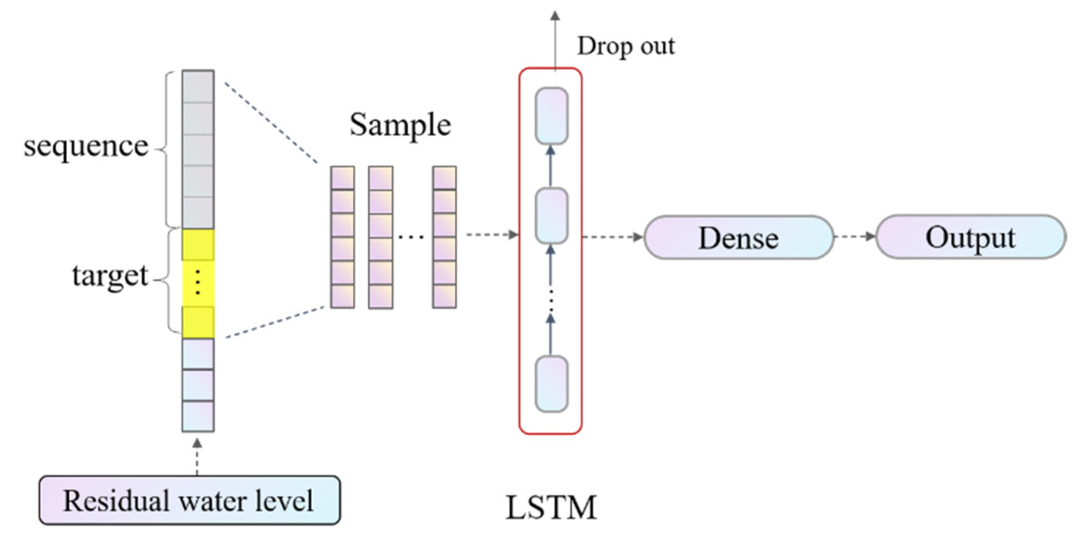
In this study, the previous time step of length m is used to forecast the residual water level for the n-hour lead time. Next, the sample data set is generated by a single-step sliding window. In this way, the time sequences of the residual water level are reorganized and transformed into a supervised learning forecast problem. The LSTM structure is implemented in Keras with the TensorFlow backend [32], and the design concept of the network follows the principle of “simple to fine,” that is, the hyperparameters are adjusted for the validation set so that the basic model with a simple structure can be updated to achieve an ideal outcome. The structure of the single-feature forecast model (SFFM) based on the LSTM network is shown in Figure 2.
2.4. Spatial Distribution Using IDW and IDWSE
IDW interpolation is commonly used in the geosciences and is usually applicable in situations with spatial distribution ambiguity. For IDW, it is assumed that weight depends only on spatial distance rather than other physical processes. The expression is:
where denotes the prediction at a nonmeasured location c; denotes the prediction at the ith observation station; q is the number of observation stations; di and are the Euclidean distance and weights between the nonmeasured location and ith observation station, respectively; and p is the power exponent, which is 2 in the calculations.
3PM is an interpolation using three adjacent observation stations to estimate the value of nonmeasured locations. Thus, it is a fast and cost-effective method in tide-station-insufficient water areas. The simulation deviation always increases from the open boundary to the bay in the semiclosed hydrodynamic model. Therefore, when the 3PM is used for interpolation, the values of interpolation points are likely to be amplified or diminished, as shown in Figure 3.
To address the abovementioned limitations, an interpolation method based on the signal energy and spatial distance (IDWSE) is proposed that is suitable for harmonic signals with linear spatial variation. The key idea of IDWSE is to correct the weak or strong weighting caused by 3PM through the signal energy ratio. First, the signal energy of the simulation deviation is calculated at each observation station (Equation (11)). Next, we identify station b with the minimum (or maximum) signal energy and calculate the signal energy multiple ki (at station b, ki = 1) of the residual observation stations relative to station b:
where and Ei denote the value and energy of the simulation deviation at the ith observation station, respectively. The values of the weights w11, w12, and w13 can be expressed as:
Finally, to prevent ki from being too large due to Ei approaching zero, the following criteria are adopted to select the interpolation method:
2.5. Evaluation Index
To evaluate the accuracy of the forecast method, the following metrics are used in this study:
- 1.
- Root-Mean-Square Error (RMSE)
RMSE is one of the most widely used criteria for evaluating the accuracy of models. RMSE is very sensitive to a large forecast error, so it can measure the forecast performance of the high and low water levels well.
- 2.
- Mean Absolute Error (MAE)
MAE is a measure to evaluate the absolute deviation between the prediction and observation. The significance for the lower and higher water level forecasts is the same, and the deviation is not magnified by the square.
- 3.
- R-Squared (R2)
R2 describes the proportion of the total variance in the observation that can be explained by the forecast model. The closer R2 is to 1, the better the regression results are.
In these equations, , , and are the actual water level, predicted water level, and mean actual water level, respectively.
3. Experiments and Results
3.1. Experiment Area
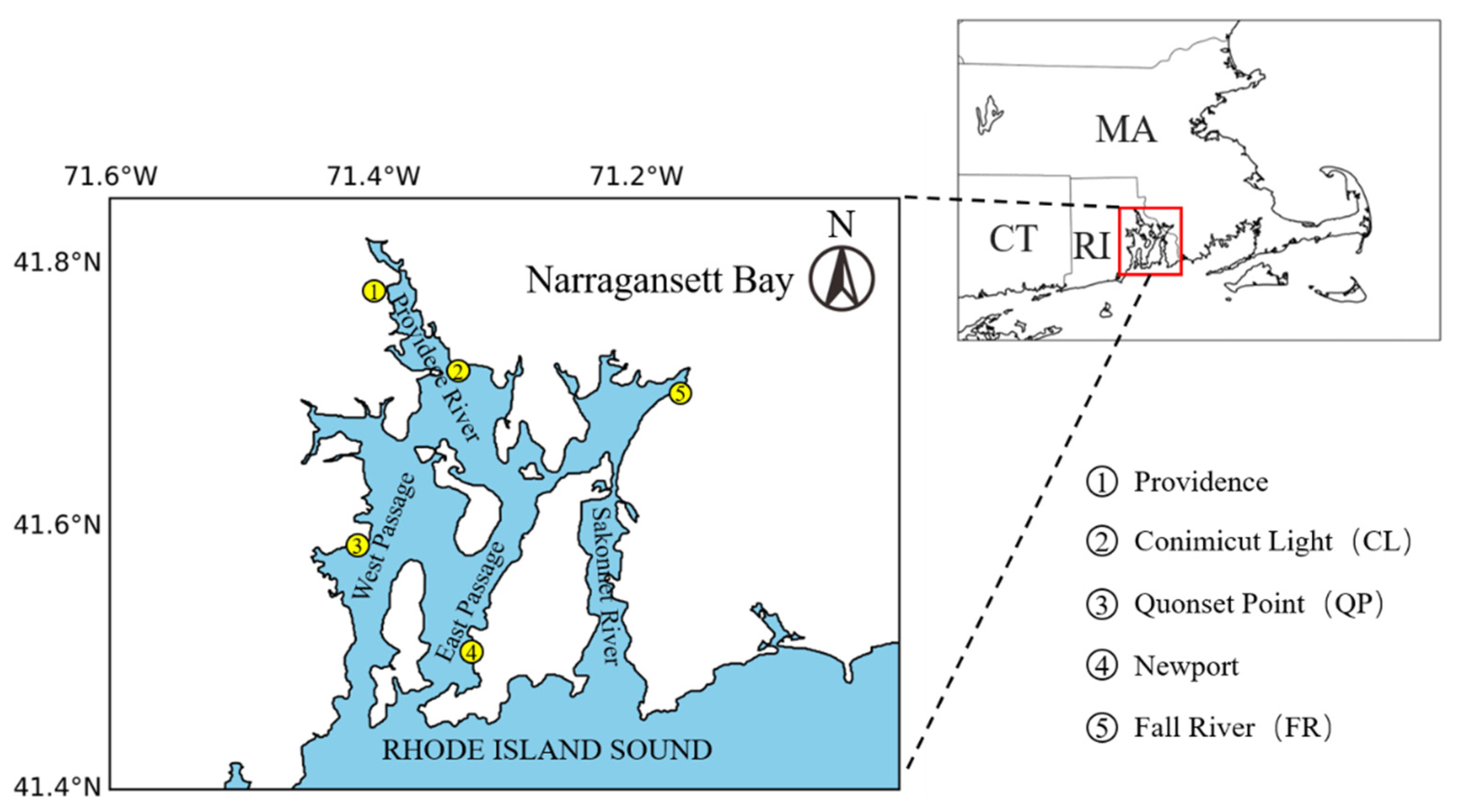
The Narragansett Bay drainage basin covers an area of 4714 km2 and is located on Rhode Island, USA. A total of 370 km2 of this area is in Narragansett Bay (40°21′–41°51′ N, 71°9′–71°30′ W), which is the largest semiclosed estuary in the northeastern United States [33]. Fresh water flowing into the bay comes mainly from the Taunton, Blackstone, and Pawtuxet Rivers. However, compared with the tide, the magnitude of river discharge (combined yearly average of 105 m3 s–1) is very small [34]. Seawater enters Narragansett Bay through three routes: The East Passage, West Passage, and Sakonnet River. The water depth in the East Passage is 16–48 m, while the West Passage is shallower (6–16 m) [35]. The diurnal range at Newport is 1.1 m and increases to 1.5 m at Providence.
3.2. Data Collection
The bathymetry and coastline data used by MIKE21 FM are derived from the products of Estuarine Bathymetry and Shoreline/Coastline Resources published by the National Oceanographic and Atmospheric Administration (NOAA), and the bathymetry datum is the mean lowest low water (MLLW). The tidal harmonic constant of the input water level at the open boundary is derived from the TPXO8_atlas tidal model published by the University of Oregon, USA [36]. The location of the five observation stations in the experimental area is shown in Figure 4. The hourly water level and meteorological observation from each station from 2013 to 2015 were selected for the experiment. To avoid introducing unnecessary errors in the datum transformation, the datum of the water level was vertically referenced to MSL in this paper.
Due to the limited number of observation stations, an experiment was designed to test the proposed method, in which Providence, Quonset Point (QP), and Fall River (FR) were used as observation stations, while Conimicut Light (CL) was regarded as the nonmeasured station to evaluate the experimental results. In addition, because of the absence of the water level at QP, six months (from April to September) of water level in 2015 were forecasted.
3.3. Forecast Results for Stationary Constituents
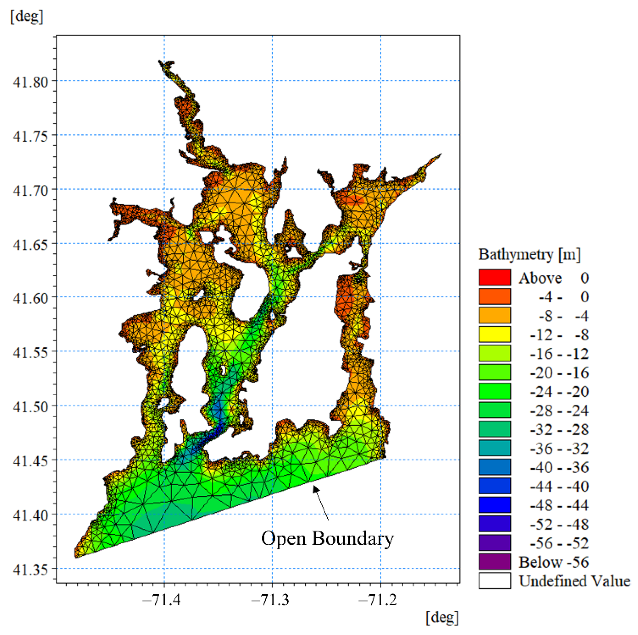
A triangular irregular network (TIN) was used to construct the bathymetric mesh. To fit the coastline better, the resolution was increased along the coastline. The value of each mesh node was interpolated using high-resolution bathymetric data, as shown in Figure 5. The spatially varying bed roughness coefficient (Manning coefficient) and eddy viscosity coefficient (Smagorinsky coefficient) were typically adjusted as important initial parameters. In the absence of empirical parameters, these two constant coefficients were tested using an iterative approach using the major astronomical tides of Newport as the calibration target. Finally, the major astronomical tidal model of Narragansett Bay (MATNB) was constructed by using the parameters in Table 2, and it will be used in subsequent forecasting work.
Unlike the residual water level, the simulation deviation is still harmonic and gradually increases from the open boundary (Newport) to the inner bay, and reaches its maximum at the head of the bay, as shown in Table 3. The M2 constituent is the main component of the simulation deviation, which means that the amplitude of M2 is underestimated in MATNB. Table 4 presents the main components of the surplus astronomical tide. Two significant constituents are SA (long-period constituent) and M4 (shallow water constituent). Due to the large spatial scale, the SA is relatively close at each station. However, the amplitude of M4 is related to the bathymetry and tends to be larger in shallow water. The hindcast of the simulation deviation and the surplus astronomical tides account for 100% of the original signal variation. The results indicate that the variations in both the simulation deviation and surplus astronomical tides at any time can be forecasted by HA.
3.4. Forecast Results for the Nonstationary Constituents
Before training the LSTM network, the sample was standardized by the z-score. Then, the two-year dataset (2013–2014) was divided into training and validation sets at a ratio of 7:3, and the next year’s residual water level was used as the testing set to verify the prediction skill of the network. The hyperparameters of the network were adjusted for the validation set. To prevent overfitting, the training stopped when the loss stopped falling. The size of each dataset and hyperparameters are shown in Table 5 and Table 6, respectively.
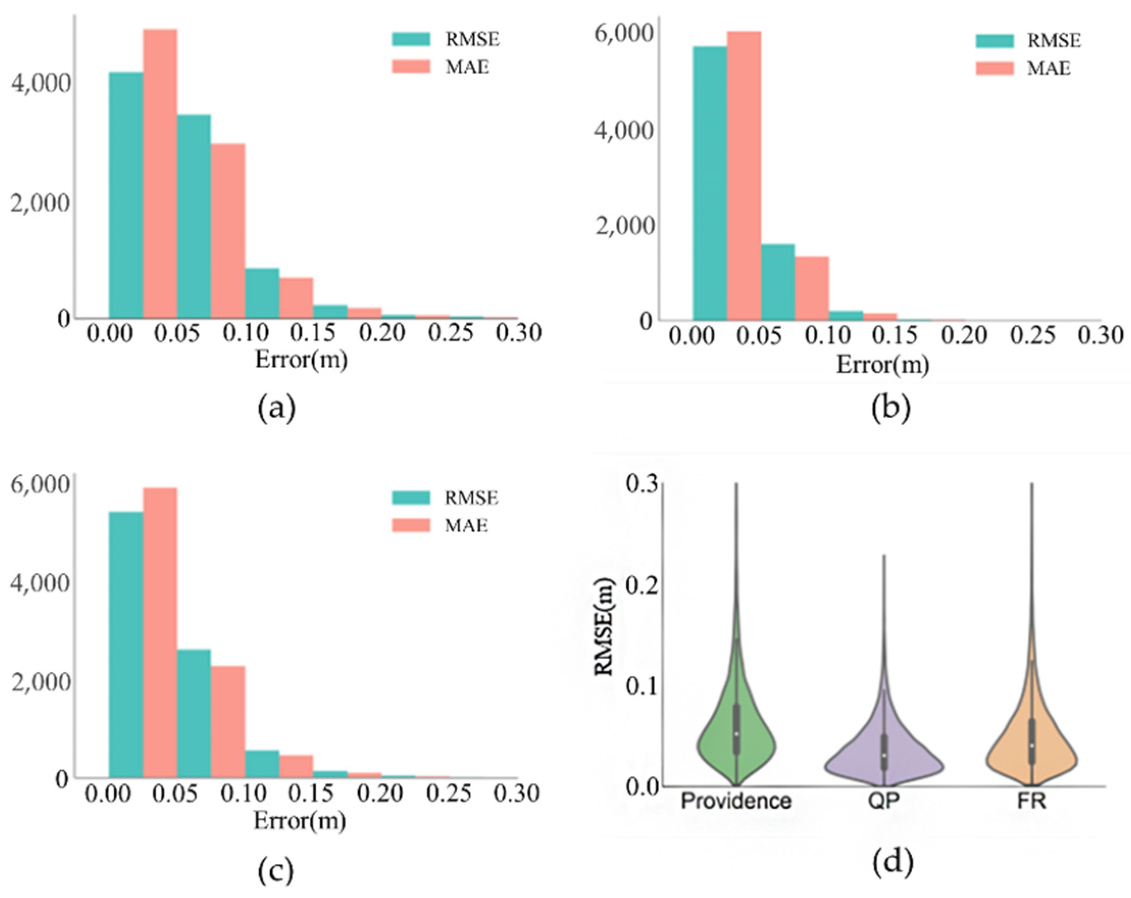
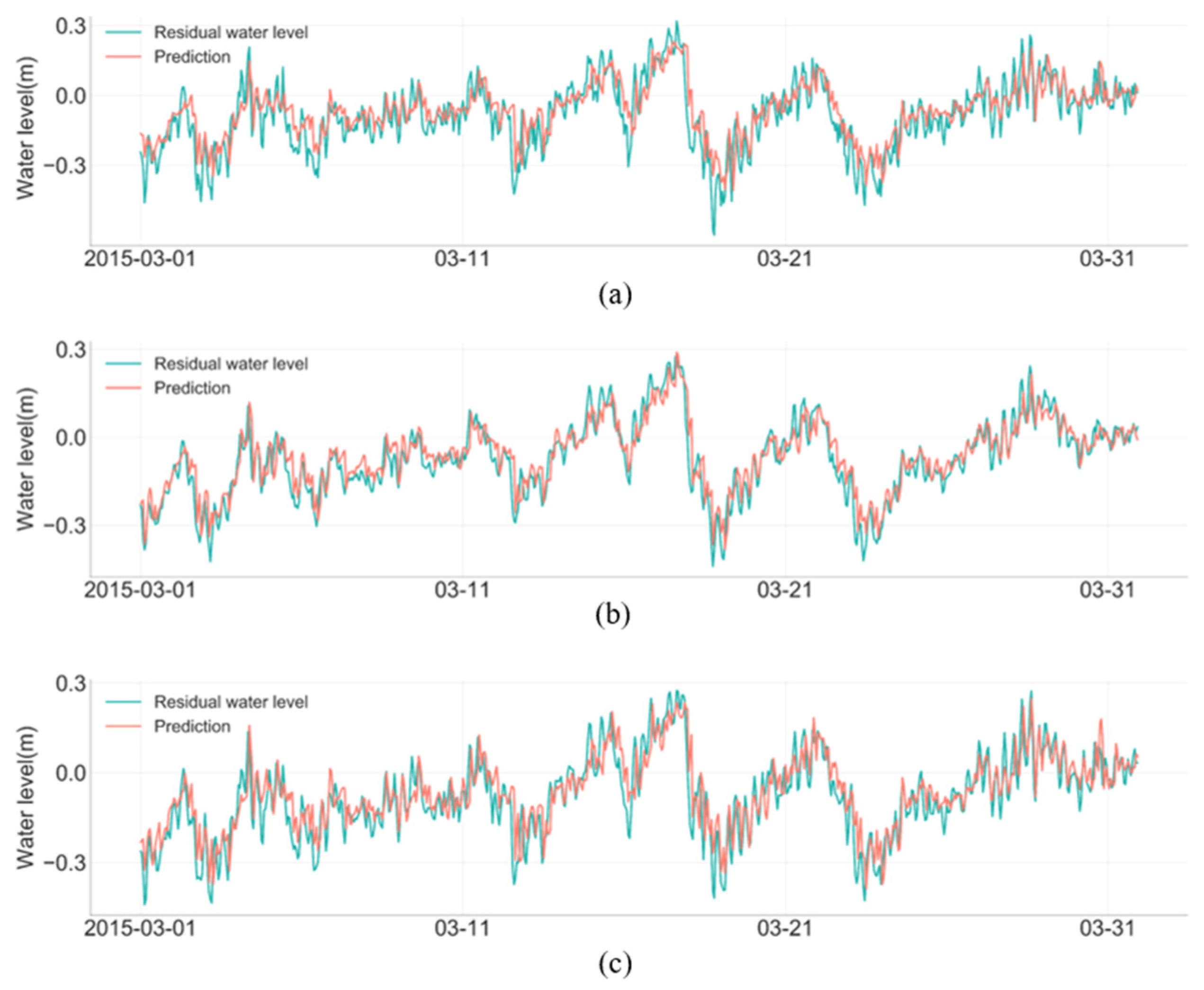
The RMSE and MAE statistics of the LSTM when the lead time (n) was equal to 3 are shown in Figure 6. The error was concentrated in the 10 cm range, with the lowest median prediction error in QP. Figure 7 further shows the performance of the LSTM network in the water level fluctuation period. The prediction at Providence does not fit the actual value well locally, showing slight underprediction of the high water level and slight overprediction of the low water level. By contrast, the performance at FR shows a moderate effect. However, the prediction performance is excellent at QP, which means that the high-frequency noise in shallow water interferes with the training and subsequently impacts the generalizability of the network. Regarding the overall forecast performance, the LSTM network still shows good stability and accuracy.
3.5. Spatial Distribution Results
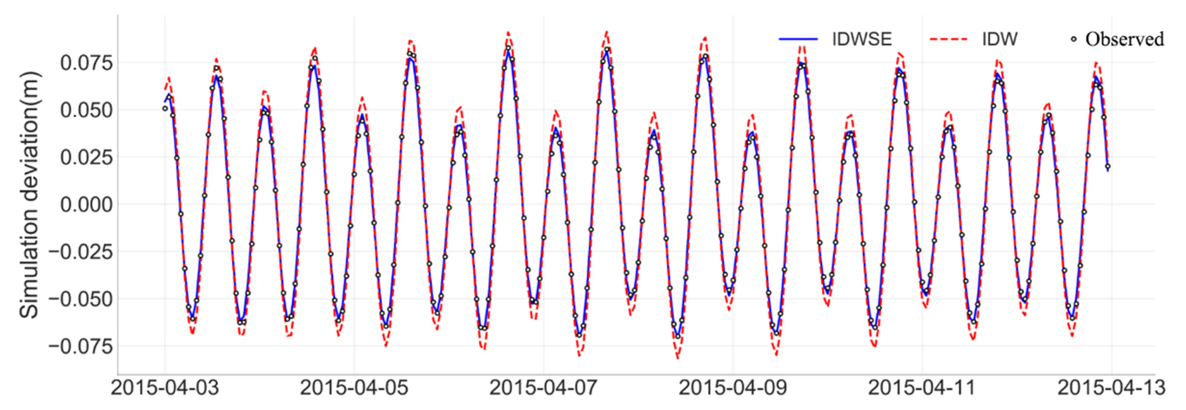
As the main constituent in the simulation deviation, the amplitude of M2 at Providence and FR is greater than that at QP, which causes weight anomalies when using 3PM interpolation. According to Table 7, the weights calculated using IDW and IDWSE have different biases. The performance of the two interpolation methods is shown in Figure 8. The curves show that the value at CL is amplified using IDW interpolation, while IDWSE interpolation solves this problem by increasing the weak weighting (QP). Furthermore, the interpolation accuracy is less sensitive to the interpolation method, which may be due to highly correlated components within the region. Despite this, IDWSE still improves the IDW interpolation accuracy slightly and proves its effectiveness.
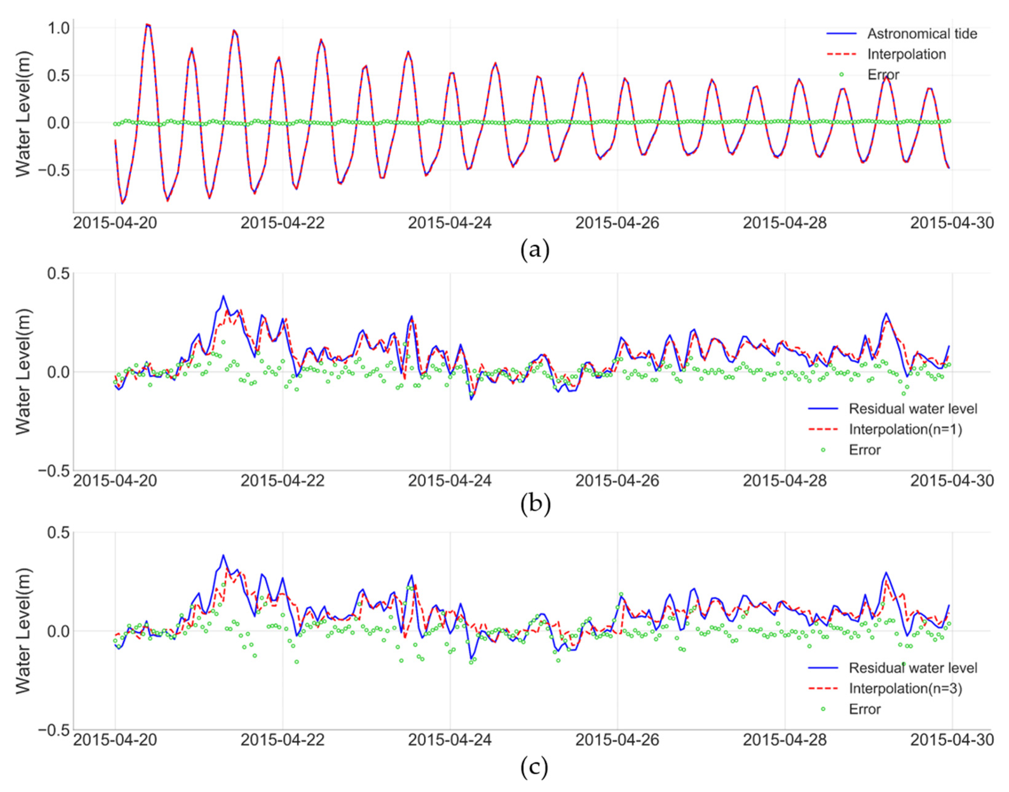
In addition to the simulation deviation, the spatial backgrounds of other constituents were not clear, so IDW was still used for spatial correction. To better illustrate the sources of error in the water level forecasting, Figure 9 shows a time series of the astronomical tides and residual water level at different lead times at CL. The astronomical tides prediction was highly correlated with the actual values, indicating that the stationary constituent was well predicted and corrected (Figure 9a). The prediction of the residual water level was closely associated with the lead times (n). When n was equal to 1, the error was essentially distributed around zero (Figure 9b), and when n was equal to 3, the errors oscillated slightly (Figure 9c). The above results demonstrate that the accuracy of the water level forecasting at CL depends mainly on the accuracy of the residual water level forecasting at observation stations.
3.6. Comparison with Assimilation Model
To verify the superiority of the proposed method, we have developed an assimilation model based on MATNB for comparison. Just like the GOMOFS, this regional water level forecasting model assimilated the hourly variation in wind and barometric field. These data are obtained from ERA5 datasets [37] provided by the European Centre for Medium-Range Weather Forecasts (ECMWF), which are available at a spatial resolution of 0.25° in longitude and latitude. Besides, eight major astronomical constituents (same as MATNB), as well as two shallow water overtides (M4 and MS4), were input at the open boundary.
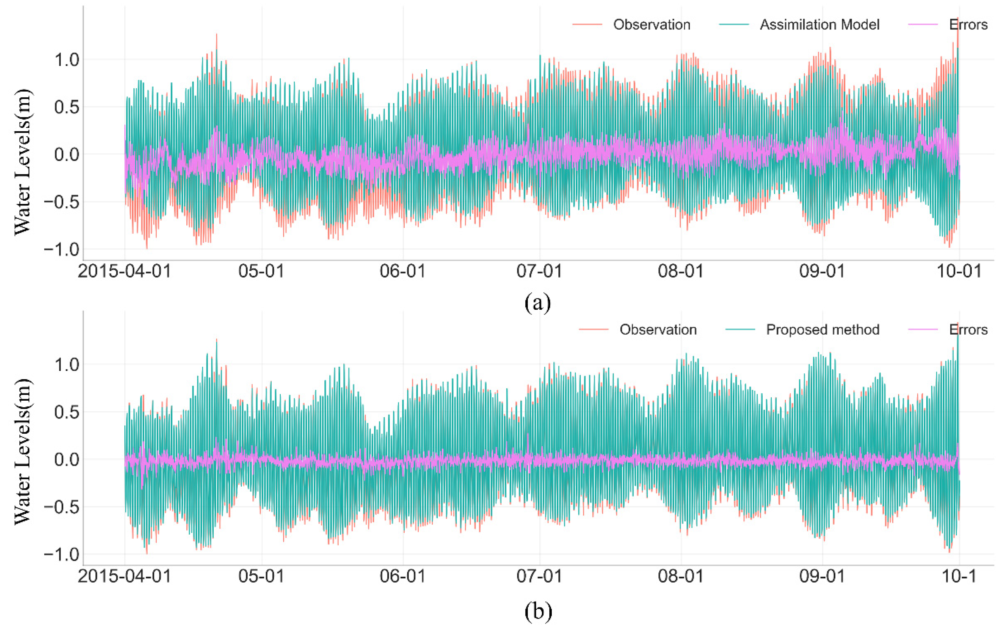
The output of the assimilation model is shown in Figure 10a. Excluding the simulation start time, the prediction accuracy of the assimilation model for the high-water level was better than that of the low water level. In estuaries, the hazards of incorrectly estimated low water levels were more significant, which can cause the vessel groundings. Due to the limitations of the hydrodynamic model, this model cannot take into account all environmental factors. In other words, the forecasting error might be further magnified under extreme conditions. However, the proposed method captured the large oscillation process during the period of fluctuation, and the prediction errors were maintained at a low level during the stationary period despite the occasional outliers (Figure 10b). According to the statistical analysis (Table 8), the RMSE was reduced from 12.3 to 5.0 cm, the MAE was reduced from 9.7 to 3.8 cm, and the R2 was increased to 0.988, indicating ideal forecast performance.
4. Discussion
4.1. Relationship between the Lead Time and Accuracy
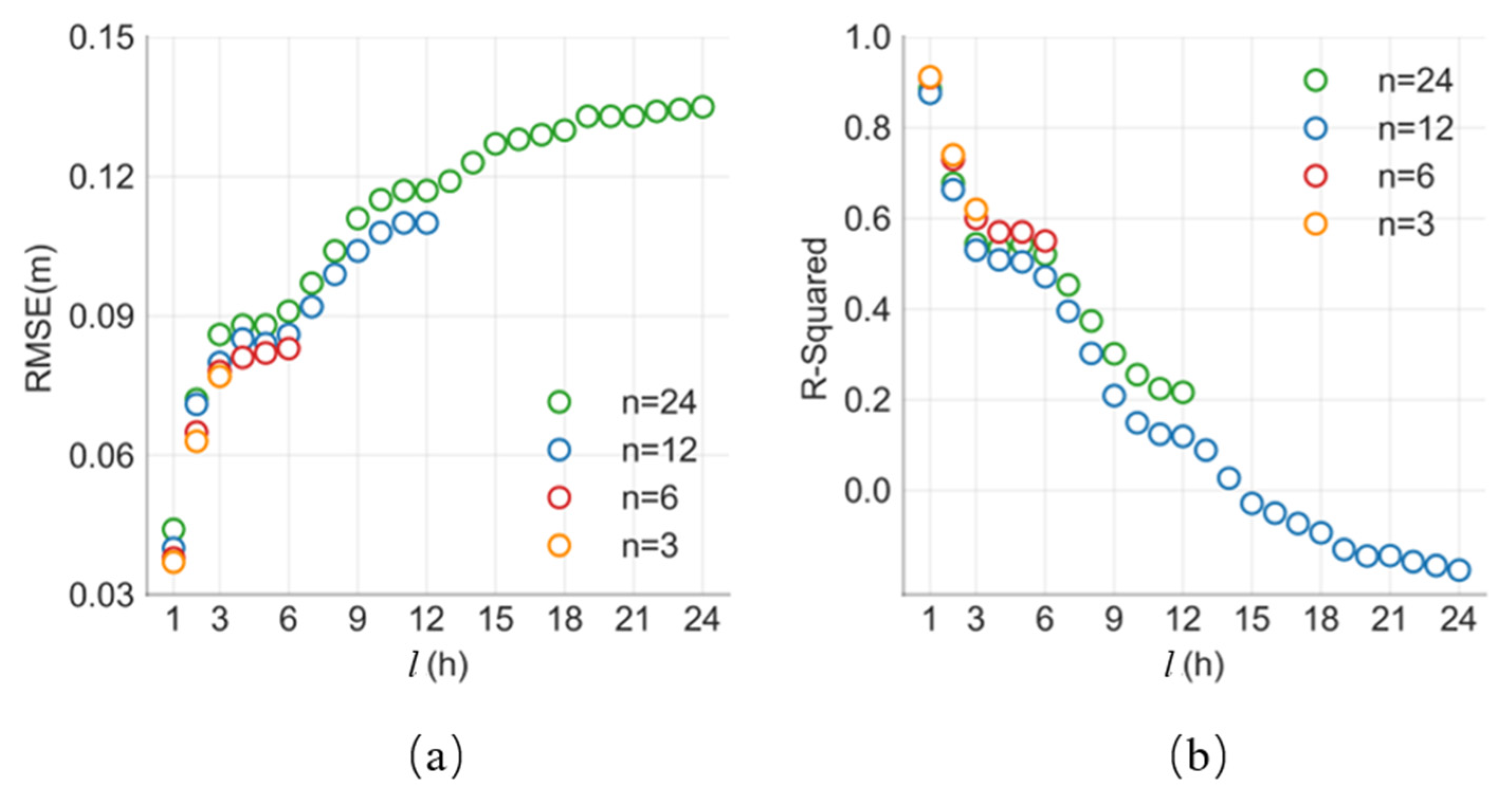
As described previously, the residual water level is the primary component of prediction error. Thus, it is necessary to analyze the relationship between the lead time and accuracy in the LSTM network. Considering the moderate efficacy of the prediction performance at FR, we predicted the hourly residual water level at FR for 3, 6, 12, and 24 h lead time. The RMSE and R2 of the prediction are illustrated in Figure 11. With increasing lead times, the overall performance of LSTM decreased slightly. Based on observations of the lth forecast time in each group, the RMSE entered the first significant growth interval with an increase of approximately 5 cm. Subsequently, the RMSE was basically unchanged when the stationary interval was 3 < l ≤ 6. The RMSE then entered a second significant growth interval at 6 < l ≤ 9, with an increase of approximately 3.5 cm. Thereafter, the RMSE increased slowly and remained near 13 cm, indicating that the prediction gradually converges. Using another precision index (R2), its prediction was highly reliable (0.91) at the first forecast time. When l = 6, the predictions could still explain over 50% of the variation in the residual water level. Of note, R2 became negative when l = 15, indicating a failure of the LSTM network.
4.2. Comparison with the Multi-Feature Forecast Model Based on the LSTM Network
Wind and barometric pressure are generally considered significant factors that cause disturbances in the water level in the coastal ocean [38]. Therefore, we evaluated the possibility of using wind and barometric pressure as features (from NOAA at the observation stations) for residual water level prediction. To this end, the above features were entered into the LSTM along with the residual water level to build a multi-feature forecast model (MFFM). The dataset construction result is shown in Table 9.
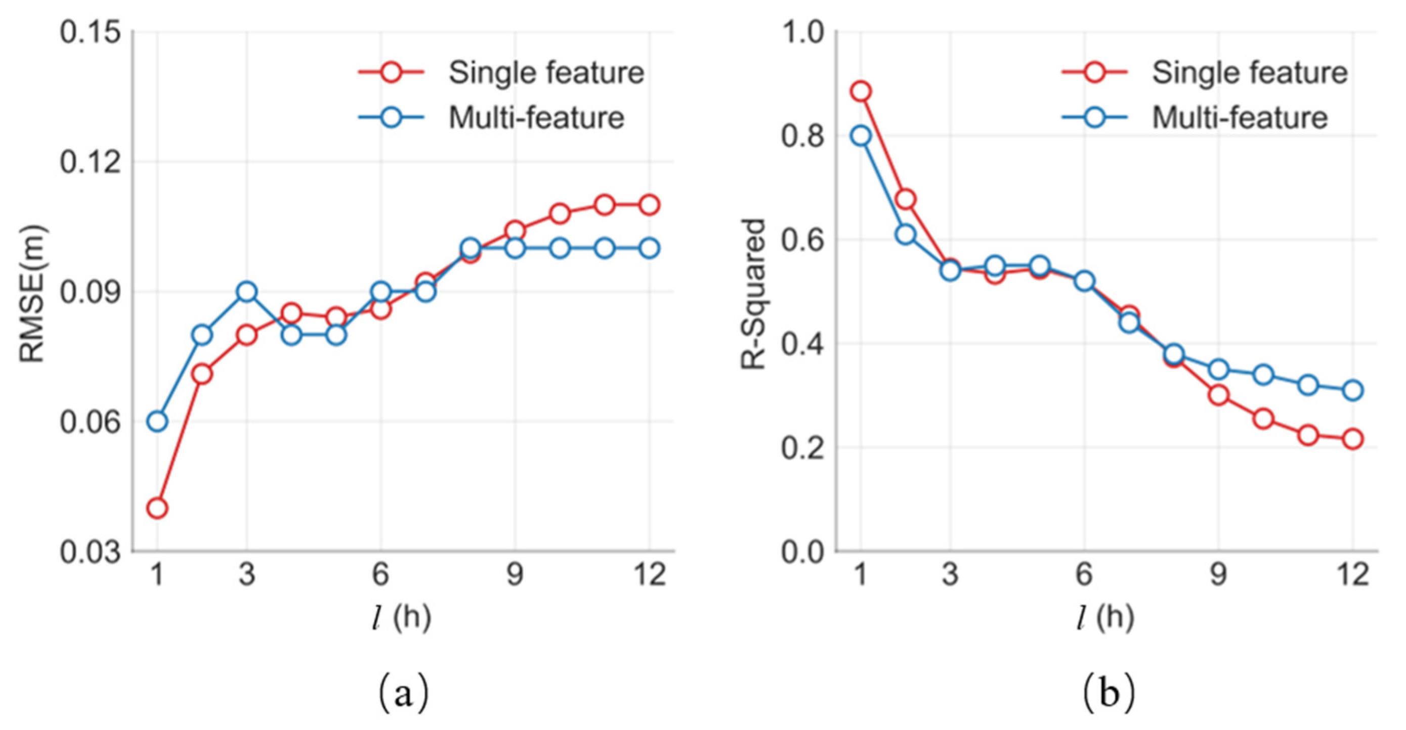
Figure 12 shows the forecast performance of these two models with a lead time of 12 h at FR. According to the variation in the RMSE and R2 curves, the interval l can be roughly divided into three parts: 0–3, 4–8, and 9–12 h. During the first interval [0, 3 h], meteorological features have a negative effect on the forecast. The RMSE of the MFFM at l = 1 reaches 6 cm, which is significantly larger than that of SFFM. During the second interval [4, 8 h], the forecast performance of these two models is almost equal. An interesting phenomenon is that the RMSE curve of MFFM does not continue to rise, but a “dent” occurs when l = 4 and 5. During the third interval [9, 12 h], the R2 of the MFFM is greater than that of SFFM by approximately 0.1, indicating that the meteorological features improve the performance of the MFFM during this period.
It is well established that a component of water level variability is due to the inverted barometer effect [39]. To further analyze the error source of MFFM, we subtracted the barometric pressure effect from the residual water level using the following hydrostatic equation [40]:
where is the residual water level produced by barometric pressure (P(t)). and g are the seawater density and acceleration due to gravity, respectively. Once the is determined, the remaining components of residual water level (ψ(t)) are assumed to be produced by wind.
We took the predicted value of l = 1 as a sequence and then used Equation (18) to obtain the 2 days’ ψ(t) of MFFM at FR (Figure 13a). As a reference, we also provided the wind speed and direction, as shown in Figure 13b. The contrasts showed that MFFM could sometimes not accurately predict the direction and magnitude of the water level variability (within the dashed frame). In fact, due to the gravity and inertia, the water level is constantly changing to maintain a dynamic balance of the regional energy. Thus, it is difficult to fully characterize this process only by using wind features, and the accuracy of the MFFM is limited to a moderate level.
5. Conclusions
To improve the accuracy of the regional water level prediction, prediction and distribution of model residuals were carried out based on the simplified hydrodynamic model output (MATNB). Experimental results at Narragansett Bay showed that the SFFM can effectively predict the residual water level in the short-term (3 h). In terms of the spatial distribution, IDWSE improved the issue of amplitude the simulation deviation at CL using three-station IDW interpolation. Compared with the assimilation model, the RMSE of this method decreased from 12.3 to 5.0 cm, and R2 increased from 0.932 to 0.988. Therefore, this method could be a viable alternative for predicting the water level in the water area with few observation stations, and it does not require additional inputs of meteorological or hydrological prediction products.
Furthermore, we considered the influence of wind and barometric pressure on the LSTM network. The results showed that the accuracy of the MFFM was limited to a moderate level. This limitation arises because it is difficult to fully characterize the dynamic equilibrium process using only wind features. Therefore, we plan to design a reasonable feature quantification scheme to improve the prediction time and accuracy of the water level in future work.
Author Contributions
Z.T. conceptualized the study and wrote the paper with the guidance and supervision of D.S., X.G. and J.X., W.S. validated the results. Y.S. provided the software. All authors have read and agreed to the published version of the manuscript.
Funding
This research was funded by the National Natural Science Foundation of China (41930535, 41830540, 52001189); National Key R&D Program of China (2018YFF0212203, 2017YFC1405006, 2018YFC1405900, 2016YFC1401210); SDUST Research Fund (2019TDJH103).
Institutional Review Board Statement
Not applicable.
Informed Consent Statement
Not applicable.
Data Availability Statement
The bathymetry, coastline, tides and meteorological data in Narragansett Bay used in this paper come from National Oceanic and Atmospheric Administration (https://www.ngdc.noaa.gov/mgg/bathymetry/relief.html, accessed on 11 December 2020; https://tidesandcurrents.noaa.gov, accessed on 11 December 2020). The ERA5 data sets used in this paper are from European Centre for Medium-Range Weather Forecasts (https://cds.climate.copernicus.eu/cdsapp#!/dataset/reanalysis-era5-single-levels?tab=overview, accessed on 11 December 2020).
Acknowledgments
We deeply thank the National Oceanic and Atmospheric Administration (https://tidesandcurrents.noaa.gov, accessed on 11 December 2020) for providing tides and meteorological data. We also thank the European Centre for Medium-Range Weather Forecasts for providing the ERA5 data sets for our study.
Conflicts of Interest
The authors declare no conflict of interest.
References
- Foreman, M.G.G.; Henry, R.F. The harmonic analysis of tidal model time series. Adv. Water Resour. 1989, 12, 109–120. [Google Scholar] [CrossRef]
- Mellor, G.L. Users Guide for a Three Dimensional, Primitive Equation, Numerical Ocean Model; Program in Atmospheric and Oceanic Sciences, Princeton University: Princeton, NJ, USA, 1998. [Google Scholar]
- Chen, C.; Liu, H.; Beardsley, R.C. An unstructured grid, finite-volume, three-dimensional, primitive equations ocean model: Application to coastal ocean and estuaries. J. Atmos. Ocean. Technol. 2003, 20, 159–186. [Google Scholar] [CrossRef]
- Bethem, T.; Burton, J.; Caldwell, T.; Evans, M.; Kittredge, R.; Lavoie, B.; Werner, J. Generation of Real-Time Narrative Summaries for Real-time Water Levels and Meteorological Observations in PORTS®. In Proceedings of the Fourth Conference on Artificial Intelligence Applications to Environmental Sciences (AMS-2005), San Diego, CA, USA, 10 January 2005. [Google Scholar]
- Pettigrew, N.R.; Roesler, C.S.; Neville, F.; Deese, H.E. An Operational Real-Time Ocean Sensor Network in the Gulf of Maine. In Proceedings of the International conference on GeoSensor Networks, Boston, MA, USA, 1–3 October 2006; pp. 213–238. [Google Scholar]
- Georgas, N.; Blumberg, A.F. Establishing confidence in marine forecast systems: The design and skill assessment of the New York Harbor Observation and Prediction System, version 3 (NYHOPS v3). In Estuarine and Coastal Modeling (2009); ASCE Press: Reston, VA, USA, 2010; pp. 660–685. [Google Scholar]
- Lanerolle, L.W.J.; Patchen, R.C.; Aikman, I.F. The Second Generation Chesapeake Bay Operational Forecast System (CBOFS2): A ROMS-Based Modeling System. In Proceedings of the 11th International Conference on Estuarine and Coastal Modeling, Monterey, CA, USA, 3–5 November 2003. [Google Scholar] [CrossRef]
- Shchepetkin, A.F.; McWilliams, J.C. The Regional Oceanic Modeling System (ROMS): A split-explicit, free-surface, topography-following-coordinate oceanic model. Ocean Model. 2005, 9, 347–404. [Google Scholar] [CrossRef]
- Peng, M.; Zhang, A.; Yang, Z. Implementation of the Gulf of Maine Operational Forecast System (GOMOFS) and the Semioperational Nowcast/Forecast Skill Assessment; National Oceanic and Atmospheric: Washington, DC, USA, 2018. [CrossRef]
- Hasan, G.M.J.; van Maren, D.S.; Ooi, S.K. Hydrodynamic modeling of Singapore’s coastal waters: Nesting and model accuracy. Ocean Model. 2016, 97, 141–151. [Google Scholar] [CrossRef]
- Wang, X.; Babovic, V. Enhancing water level prediction through model residual correction based on Chaos theory and Kriging. Int. J. Numer. Methods Fluids 2014, 75, 42–62. [Google Scholar] [CrossRef]
- Karri, R.R.; Wang, X.; Gerritsen, H. Ensemble based prediction of water levels and residual currents in Singapore regional waters for operational forecasting. Environ. Model. Softw. 2014, 54, 24–38. [Google Scholar] [CrossRef]
- Sun, Y.; Babovic, V.; Chan, E.S. Artificial neural networks as routine for error correction with an application in Singapore regional model. Ocean Dyn. 2012, 62, 661–669. [Google Scholar] [CrossRef]
- Sun, Y.; Sisomphon, P.; Babovic, V.; Chan, E.S. Efficient data assimilation method based on chaos theory and Kalman filter with an application in Singapore Regional Model. J. Hydro-Environ. Res. 2010, 3, 85–95. [Google Scholar] [CrossRef]
- Kurniawan, A.; Ooi, S.K.; Babovic, V. Improved sea level anomaly prediction through combination of data relationship analysis and genetic programming in Singapore Regional Waters. Comput. Geosci. 2014, 72, 94–104. [Google Scholar] [CrossRef]
- Hochreiter, S.; Schmidhuber, J. Long Short-Term Memory. Neural Comput. 1997, 9, 1735–1780. [Google Scholar] [CrossRef] [PubMed]
- Liang, C.; Li, H.; Lei, M.; Du, Q. Dongting Lake Water Level Forecast and Its Relationship with the Three Gorges Dam Based on a Long Short-Term Memory Network. Water 2018, 10, 1389. [Google Scholar] [CrossRef] [Green Version]
- Le, X.-H.; Ho, H.V.; Lee, G.; Jung, S. Application of long short-term memory (LSTM) neural network for flood forecasting. Water 2019, 11, 1387. [Google Scholar] [CrossRef] [Green Version]
- Song, T.; Ding, W.; Wu, J.; Liu, H.; Zhou, H.; Chu, J. Flash Flood Forecasting Based on Long Short-Term Memory Networks. Water 2019, 12, 109. [Google Scholar] [CrossRef] [Green Version]
- Yang, C.H.; Wu, C.H.; Hsieh, C.M. Long Short-Term Memory Recurrent Neural Network for Tidal Level Forecasting. IEEE Access 2020, 8, 159389–159401. [Google Scholar] [CrossRef]
- Singh, K.; Jardak, M.; Sandu, A.; Bowman, K.; Lee, M.; Jones, D. Construction of non-diagonal background error covariance matrices for global chemical data assimilation. Geosci. Model Dev. 2011, 4, 299–316. [Google Scholar] [CrossRef] [Green Version]
- Lu, G.Y.; Wong, D.W. An adaptive inverse-distance weighting spatial interpolation technique. Comput. Geosci. 2008, 34, 1044–1055. [Google Scholar] [CrossRef]
- Cressie, N. The origins of kriging. Math. Geol. 1990, 22, 239–252. [Google Scholar] [CrossRef]
- Ika, N.; Purnama, S.; Hartono. The determination of groundwater flow system using several deterministicand classical methods in Limboto-Gorontalo Lowland, Gorontalo Province. IOP Conf. Ser. Earth Environ. Sci. 2020, 485. [Google Scholar] [CrossRef]
- Symonds, A.M.; Vijverberg, T.; Post, S.; Spek, B.J.V.D.; Sokolewicz, M. Comparison between Mike 21 FM, Delft3D and Delft3D FM Flow Models of Western Port Bay, Australia. Coast. Eng. Proc. 2017, 11. [Google Scholar] [CrossRef]
- Syed, Z.; Choi, G.; Byeon, S. A Numerical Approach to Predict Water Levels in Ungauged Regions—Case Study of the Meghna River Estuary, Bangladesh. Water 2018, 10, 110. [Google Scholar] [CrossRef] [Green Version]
- Mahdavi, A.H.; Sharghi, H.A. Numerical Investigation of Storm Surge in Kong Port in the Persian Gulf. engrXiv 2019. [Google Scholar] [CrossRef] [Green Version]
- Fadlillah, L.N.; Widyastuti, M.; Sunarto; Marfai, M.A. Comparison of tidal model using mike21 and delft3d-flow in part of Java Sea, Indonesia. IOP Conf. Ser. Earth Environ. Sci. 2020, 451. [Google Scholar] [CrossRef] [Green Version]
- Warren, I.R.; Bach, H.K. MIKE 21: A modelling system for estuaries, coastal waters and seas. Environ. Softw. 1992, 7, 229–240. [Google Scholar] [CrossRef]
- Godin, G. The Analysis of Tides; University of Toronto Press: Toronto, ON, Canada, 1972; Volume xxi. [Google Scholar]
- Sherstinsky, A. Fundamentals of Recurrent Neural Network (RNN) and Long Short-Term Memory (LSTM) network. Physica D 2020, 404, 132306. [Google Scholar] [CrossRef] [Green Version]
- Brownlee, J. Deep Learning With Python: Develop Deep Learning Models on Theano and TensorFlow Using Keras; Machine Learning Mastery: San Francisco, CA, USA, 2016. [Google Scholar]
- Ries, K. Estimating surface-water runoff to Narragansett Bay, Rhode Island and Massachusetts. Water-Resour. Investig. Rep. 1990, 89, 4164. [Google Scholar] [CrossRef]
- Gordon, R.B.; Spaulding, M.L. Numerical simulations of the tidal and wind-driven circulation in Narragansett Bay. Estuar. Coast. Shelf Sci. 1987, 24, 611–636. [Google Scholar] [CrossRef]
- Kincaid, C.; Bergondo, D.; Rosenberger, K. The Dynamics of Water Exchange Between Narragansett Bay and Rhode Island Sound. In Science for Ecosystem-Based Management: Narragansett Bay in the 21st Century; Desbonnet, A., Costa-Pierce, B.A., Eds.; Springer: New York, NY, USA, 2008; pp. 301–324. [Google Scholar]
- Egbert, G.D.; Erofeeva, S.Y. Efficient Inverse Modeling of Barotropic Ocean Tides. J. Atmos. Ocean. Technol. 2002, 19, 183–204. [Google Scholar] [CrossRef] [Green Version]
- Hersbach, H.; Bell, B.; Berrisford, P.; Hirahara, S.; Horányi, A.; Muñoz-Sabater, J.; Nicolas, J.; Peubey, C.; Radu, R.; Schepers, D. The ERA5 global reanalysis. Q. J. R. Meteorol. Soc. 2020, 146, 1999–2049. [Google Scholar] [CrossRef]
- David, S.-M.; Arnoldo, V.-L. Sea-Level Slopes and Volume Fluxes Produced by Atmospheric Forcing in Estuaries: Chesapeake Bay Case Study. J. Coast. Res. 2008, 24, 208–217. [Google Scholar] [CrossRef] [Green Version]
- Smith, N.P. Meteorological forcing of coastal waters by the inverse barometer effect. Estuar. Coast. Mar. Sci. 1979, 8, 149–156. [Google Scholar] [CrossRef]
- Gill, A.E. Atmosphere-Ocean Dynamics; Academic Press: Cambridge, MA, USA, 1982; p. 662. [Google Scholar]
Figure 1.
Flowchart of the proposed method.

Figure 2.
Structure of the single-feature forecast model (SFFM) based on the long short-term memory (LSTM) network.
Figure 2.
Structure of the single-feature forecast model (SFFM) based on the long short-term memory (LSTM) network.

Figure 3.
When using three-point interpolation (3PM) based on inverse distance weighting (IDW), the value of interpolating point I1 may be amplified if it is closer to the two observation stations along the coastline, and the value of interpolating point I2 may be diminished if it is closer to the two observation stations far away from the coastline.

Figure 4.
Location of Narragansett Bay and observation stations.

Figure 5.
Extent, mesh (5835 nodes), and bathymetry of major astronomical tidal model of Narragansett Bay (MATNB).
Figure 5.
Extent, mesh (5835 nodes), and bathymetry of major astronomical tidal model of Narragansett Bay (MATNB).

Figure 6.
Root-mean-square error (RMSE) and mean absolute error (MAE) of the residual water level prediction (n = 3) in the testing set at (a) Providence, (b) Quonset Point (QP), and (c) Fall River (FR); (d) density of RMSE at each station.
Figure 6.
Root-mean-square error (RMSE) and mean absolute error (MAE) of the residual water level prediction (n = 3) in the testing set at (a) Providence, (b) Quonset Point (QP), and (c) Fall River (FR); (d) density of RMSE at each station.

Figure 7.
Performance (n = 3) of LSTM network in the water level fluctuation period at (a) Providence, (b) QP, and (c) FR.
Figure 7.
Performance (n = 3) of LSTM network in the water level fluctuation period at (a) Providence, (b) QP, and (c) FR.

Figure 8.
Simulation deviation using IDW and IDWSE interpolation at Conimicut Light (CL).

Figure 9.
Predictions of (a) astronomical tide, (b) residual water level (n = 1), and (c) residual water level (n = 3) at CL, obtained by interpolation from Providence, FR, and QP.
Figure 9.
Predictions of (a) astronomical tide, (b) residual water level (n = 1), and (c) residual water level (n = 3) at CL, obtained by interpolation from Providence, FR, and QP.

Figure 10.
Time series of the observed water level at CL compared with (a) the assimilation model and (b) the proposed method (n = 3).
Figure 10.
Time series of the observed water level at CL compared with (a) the assimilation model and (b) the proposed method (n = 3).

Figure 11.
The (a) RMSE and (b) R2 of the SFFM for 3, 6, 12, and 24 h lead times at FR.

Figure 12.
The (a) RMSE and (b) R2 of the SFFM and multi-feature forecast model (MFFM) with a lead time of 12 h at FR.
Figure 12.
The (a) RMSE and (b) R2 of the SFFM and multi-feature forecast model (MFFM) with a lead time of 12 h at FR.

Figure 13.
Time series of (a) ψ(t) and (b) wind features at FR on 11 and 12 November 2015.


Table 1.
Definition and properties of the water level constituents.
| Constituent | Definition | Property |
|---|---|---|
| Astronomical tides: Hast | Significant astronomical tide | Stationary |
| Simulated values of the major astronomical tides: Hsimu | M2, S2, N2, K2, K1, O1, P1, Q1 | Stationary |
| Actual values of the major astronomical tides: Hmain | M2, S2, N2, K2, K1, O1, P1, Q1 | Stationary |
| Simulation deviation: εmodel | Hmain − Hsimu | Stationary |
| Surplus astronomical tides: Hrt | Hast − Hmain | Stationary |
| Residual water level: R | Observation (H) − Hast | Nonstationary |
Table 2.
Main parameters of MANTB.
| Parameters | Value |
|---|---|
| Time | From 1 January 2015 to 31 December 2015; time step: 3600 s |
| Eddy viscosity | Smagorinsky formulation, constant value: 0.28 |
| Density | Barotropic |
| Bed resistance | Manning coefficient: 45 |
| Boundary conditions | Water level including M2, S2, N2, K2, K1, O1, P1, Q1 |
Table 3.
Harmonic constants of the simulation deviation at each station.
| Tidal Constituent | Providence (100%) 1 | QP (100%) | Newport (100%) | FR (100%) | ||||
|---|---|---|---|---|---|---|---|---|
| Amplitude (cm) | Phase (deg) | Amplitude (cm) | Phase (deg) | Amplitude (cm) | Phase (deg) | Amplitude (cm) | Phase (deg) | |
| Q1 | 0.1 | 236.3 | 0.1 | 232.2 | 0.6 | 174.7 | 0.1 | 224.1 |
| O1 | 0.7 | 28.1 | 0.7 | 24.2 | 0.1 | 47.9 | 0.7 | 21.6 |
| P1 | 0.3 | 92.1 | 0.4 | 78.7 | 0.7 | 85.4 | 0.4 | 101.4 |
| K1 | 1.7 | 48.3 | 1.6 | 43.1 | 1.4 | 38.0 | 1.5 | 46.3 |
| N2 | 1.3 | 40.4 | 0.9 | 32.2 | 0.9 | 355.8 | 1.5 | 46.0 |
| M2 | 7.8 | 46.6 | 5.3 | 39.1 | 4.3 | 44.1 | 8.3 | 49.7 |
| S2 | 2.1 | 56.5 | 1.6 | 43.0 | 1.5 | 46.8 | 2.0 | 56.1 |
| K2 | 0.8 | 253.1 | 1.0 | 257.0 | 1.0 | 261.0 | 1.0 | 254.9 |
1 Hindcast of the simulation deviation accounting for 100% of the original signal variation.
Table 4.
Harmonic constants of the surplus astronomical tides at each station.
| Tidal Constituent | Providence (100%) 1 | QP (100%) | Newport (100%) | FR (100%) | ||||
|---|---|---|---|---|---|---|---|---|
| Amplitude (cm) | Phase (deg) | Amplitude (cm) | Phase (deg) | Amplitude (cm) | Phase (deg) | Amplitude (cm) | Phase (deg) | |
| SA | 9.9 | 219.1 | 8.8 | 224.2 | 8.9 | 230.1 | 9.1 | 224.0 |
| M4 | 9.1 | 60.5 | 6.1 | 48.1 | 5.1 | 37.2 | 9.0 | 64.4 |
| MN4 | 3.9 | 12.4 | 2.6 | 0.8 | 2.2 | 351.6 | 3.8 | 17.4 |
| S1 | 3.4 | 333.1 | 2.3 | 341.2 | 1.8 | 335.4 | 3.1 | 344.3 |
| MU2 | 2.7 | 1.6 | 2.5 | 354.8 | 2.4 | 349.0 | 2.7 | 3.4 |
| M6 | 2.5 | 307.3 | 0.7 | 267.0 | 0.5 | 218.1 | 1.9 | 333.3 |
| MS4 | 2.4 | 142.2 | 1.6 | 121.9 | 1.3 | 107.5 | 2.5 | 145.6 |
| NU2 | 2.4 | 352.0 | 2.2 | 348.4 | 2.4 | 349.0 | 2.4 | 353.2 |
1 Hindcast of the surplus astronomical tides accounting for 100% of the original signal variation.
Table 5.
Dataset size, units: Group.
| Dataset | Providence | Quonset Point | Fall River |
|---|---|---|---|
| Training | 12,122 | 9338 | 12,148 |
| Validation | 5196 | 4003 | 5207 |
| Testing | 8733 | 7461 | 8733 |
Table 6.
The hyperparameters of the LSTM network.
| Hyperparameters | Number of LSTM Layer | Neuron Numbers | Drop Out | Epoch | Gradient Descent Optimizer | Learning Rate | Activity Function of Dense Layer |
|---|---|---|---|---|---|---|---|
| Value | 1 | 64 | 0.2 | 100 | RMSprop | 0.001 | ReLu |
Table 7.
The weight calculated by IDW and IDWSE.
| Method | Providence (11 km) 1 | QP (15 km) | FR (15 km) |
|---|---|---|---|
| IDW | 0.48 | 0.26 | 0.26 |
| IDWSE | 0.26 | 0.61 | 0.13 |
1 Distance measured from CL, and the same is true for the other stations.
Table 8.
Comparison of the evaluation metrics between the two methods.
| Method | RMSE (cm) | MAE (cm) | R2 |
|---|---|---|---|
| Assimilation model | 12.3 | 9.7 | 93.2% |
| Proposed | 5.0 | 3.8 | 98.8% |
| Improvement | 59.3% | 60.8% | 5.6% |
Table 9.
Converting features to a dataset for the LSTM network.
| Feat1 (t − m) ~Feat1 (t − 1) 1 | Feat2 (t − m) ~Feat2 (t − 1) | Feat3 (t − m) ~Feat3 (t − 1) | Feat4 (t − m) ~Feat4 (t − 1) | Feat1(t)~ Feat1 (t + n − 1) |
|---|---|---|---|---|
| Residual water level | Wind speed | Wind direction | Barometric pressure | Residual water level |
1 Feat1 (t − m) ~ Feat1 (t − 1) refers to feature 1 from time t − m to t − 1, and the same is true for the other features.
Publisher’s Note: MDPI stays neutral with regard to jurisdictional claims in published maps and institutional affiliations. |
© 2021 by the authors. Licensee MDPI, Basel, Switzerland. This article is an open access article distributed under the terms and conditions of the Creative Commons Attribution (CC BY) license (http://creativecommons.org/licenses/by/4.0/).
Share and Cite
MDPI and ACS Style
Tu, Z.; Gao, X.; Xu, J.; Sun, W.; Sun, Y.; Su, D. A Novel Method for Regional Short-Term Forecasting of Water Level. Water 2021, 13, 820. https://doi.org/10.3390/w13060820
AMA Style
Tu Z, Gao X, Xu J, Sun W, Sun Y, Su D. A Novel Method for Regional Short-Term Forecasting of Water Level. Water. 2021; 13(6):820. https://doi.org/10.3390/w13060820
Chicago/Turabian StyleTu, Zejie, Xingguo Gao, Jun Xu, Weikang Sun, Yuewen Sun, and Dianpeng Su. 2021. "A Novel Method for Regional Short-Term Forecasting of Water Level" Water 13, no. 6: 820. https://doi.org/10.3390/w13060820
Note that from the first issue of 2016, this journal uses article numbers instead of page numbers. See further details here.