
Improving Mean Annual Precipitation Prediction Incorporating Elevation and Taking into Account Support Size


1
National Research Council of Italy—Institute for Agricultural and Forest Systems in the Mediterranean (ISAFOM), 87036 Rende (CS), Italy
2
National Research Council of Italy—Research Institute for Geo-Hydrological Protection (IRPI), 87036 Rende (CS), Italy
*
Author to whom correspondence should be addressed.
Water 2021, 13(6), 830; https://doi.org/10.3390/w13060830
Submission received: 22 February 2021
/
Revised: 14 March 2021
/
Accepted: 16 March 2021
/
Published: 18 March 2021
(This article belongs to the Special Issue Modelling Precipitation in Space and Time)
Abstract
:Accounting for secondary exhaustive variables (such as elevation) in modelling the spatial distribution of precipitation can improve their estimate accuracy. However, elevation and precipitation data are associated with different support sizes and it is necessary to define methods to combine such different spatial data. The paper was aimed to compare block ordinary cokriging and block kriging with an external drift in estimating the annual precipitation using elevation as covariate. Block ordinary kriging was used as reference of a univariate geostatistical approach. In addition, the different support sizes associated with precipitation and elevation data were also taken into account. The study area was the Calabria region (southern Italy), which has a spatially variable Mediterranean climate because of its high orographic variability. Block kriging with elevation as external drift, compared to block ordinary kriging and block ordinary cokriging, was the most accurate approach for modelling the spatial distribution of annual mean precipitation. The three measures of accuracy (MAE, mean absolute error; RMSEP, root-mean-squared error of prediction; MRE, mean relative error) have the lowest values (MAE = 112.80 mm; RMSEP = 144.89 mm, and MRE = 0.11), whereas the goodness of prediction (G) has the highest value (75.67). The results clearly indicated that the use of an exhaustive secondary variable always improves the precipitation estimate, but in the case of areas with elevations below 120 m, block cokriging makes better use of secondary information in precipitation estimation than block kriging with external drift. At higher elevations, the opposite is always true: block kriging with external drift performs better than block cokriging. This approach takes into account the support size associated with precipitation and elevation data. Accounting for elevation allowed to obtain more detailed maps than using block ordinary kriging. However, block kriging with external drift produced a map with more local details than that of block ordinary cokriging because of the local re-evaluation of the linear regression of precipitation on block estimates.
1. Introduction
Assessing the spatial distribution of precipitation is crucial for water resource management and, in particular, for facing the challenges of agriculture and food production [1]. The accurate modelling of precipitation is a well-known topic and it essentially consists in predicting the precipitation over more or less areas, depending on the objectives of such modelling, from a few sparse measuring stations with good confidence [2,3,4].
The use of remote sensing data to indirectly obtain comprehensive precipitation can be a feasible alternative to direct measurements, but the accuracy and resolution of precipitation may not be adequate for the intended use [5].
Precipitation varies more or less continuously in the geographical space and is suitable to be modelled as an intrinsic stationary process by using the methods of geostatistics [3,6,7]. Consequently, many different geostatistical methods have been developed for characterizing and modelling precipitation, both simple ones that only use precipitation measurements at fixed points and more complex ones that also use extensive information as covariates for spatial interpolation [3,8,9,10]. Choosing an interpolation method for a given dataset and study area is a key issue in many cases. In areas with low relief and abundant data from evenly distributed precipitation gauges, most interpolation methods give similar results [11]. Unfortunately, such conditions are rarely found and, especially in mountainous areas with sparse data, implicit or explicit assumptions about the variation among measured points may differ significantly even at relatively small scales [11,12,13]. Furthermore, the interpolation of point data does not end with the production of a map, but allows for inferences to be made and knowledge about the precipitation process to be improved. Therefore, great caution is needed when using information from precipitation atlases based only on statistical relationships [14]. There are different methods that may combine regression analysis and distance-based weighted averages producing smooth surfaces [15,16,17,18]. In these methods, the key difference among them is in the criteria used in determining the weights of point data in relation to distance. These criteria may include simple distance relations as in inverse distance weighting methods [19], variance minimization as in different types of kriging algorithms [20], or curvature minimization and the application of smoothness criteria as in splining [21,22].
Compared to using only precipitation measurements, it has been shown that the use of exhaustive auxiliary variables as covariates in multivariate geostatistics can improve the accuracy of precipitation estimation [23]. Such an improvement depends on the explanatory relationship between precipitation and covariates. Therefore, interpolating point data may allow to understand factors controlling the distribution of precipitation [7,14]. There are many studies of multivariate geostatistics using covariates as radar imagery or topographic attributes [23,24,25,26,27].
The precipitation–elevation relationship is perhaps the most widely used, and it has been shown how elevation strongly controls the variability of precipitation at the small scale of monthly, annual, or interannual precipitations [2,12,23,24,25,28,29,30,31]. Moreover, the correlation between elevation and precipitation becomes stronger as the time aggregation increases [31], and Goovaerts [23] reported that implementing the elevation as background information can improve the interpolation performance on a monthly and yearly time scale. However, it may not be possible to capture such a relationship because it also depends on the spatial scale [32].
However, elevation (or any other topographic attribute) and precipitation data are associated with different support sizes, which for precipitation can be considered punctual (very small surface unit), while for elevation it depends on the resolution of the digital elevation model and the support size can certainly not be considered punctual. Usually, in multivariate geostatistics applications, different types of data are used without regard to the original size of the support with which they are associated. Instead, to combine such different spatial data, it is necessary to define methods to take into account the underlying uncertainties and change of support [33]. Generally, when applying statistical methods there is a tendency to overlook support problems, whereas in the application of geostatistics this has been taken into account.
The use of elevation as covariate for estimating precipitation at annual temporal scale has been described and, theoretically, it should move from the academic and research domains to operational use. However, there are two geostatistical estimators that are designed to incorporate exhaustively secondary information: cokriging and kriging with external drift [34]. The main differences between them consists in how the covariate (collocated) datum is handled: in cokriging that datum influences the primary cokriging estimate, whereas in kriging with external drift (KED) the secondary datum provides information only about the primary trend at a given location. In addition, in KED the secondary information tends to influence strongly the estimate, whereas cokriging accounts for the global linear correlation between primary and secondary variables as captured by the cross variogram [34]. Assessing which of the two geostatistical methods best models mean annual precipitation is certainly an important research issue. Moreover, further advance on the problem of the different support sizes associated with precipitation and elevation data needs to be considered appropriately.
The main objective of this paper was comparing block ordinary cokriging and block kriging with an external drift in estimating the mean annual precipitation using elevation as covariate. As reference of a univariate geostatistical approach, block ordinary kriging was used. The different support sizes associated with precipitation and elevation data were also taken into account.
2. Materials and Methods
2.1. Study Area and Data
Calabria region is located at the southern part of the Italian peninsula (Figure 1) and has a surface area of 15,080 km2. The mean elevation is 597 m above sea level (a.s.l.), whereas its highest elevation is 2266 m a.s.l. Calabria region is one of the most mountainous Italian areas, but it does not have many high peaks (Figure 1): 42% of the regional area is classified as mountain (elevation greater than 500 m a.s.l.), 49% hills (elevation between 50 and 500 m a.s.l.), and only 9% plain (elevation less than 50 m a.s.l.).
Calabria region, as a result of its geographic position within the Mediterranean sea and its orography (Figure 1), has a climate typically Mediterranean [35], with warm air currents coming from Africa and high temperatures affecting the Ionian side of Calabria, which leads to short and heavy precipitation. The Tyrrhenian side of Calabria is affected by western air current, which causes temperatures to be milder and precipitation amount to be higher on the mountains than on the Ionian side. The inner areas of the region have cold and snowy winters, and fresh summers with some precipitation [36].
The data used in this study are a set of mean annual precipitation series relative to the period 1921–2010 collected by the Multi-Risk Functional Centre of the Regional Agency for Environment Protection. From a long-term database were selected 183 precipitation series having more than 50 years of observations, and the mean annual precipitation was calculated for each precipitation gauge.
The elevation data were obtained from a digital elevation model (DEM) with 80 m × 80 m cell size.
2.2. Geostatistical Approach
Here, only a very brief introduction to the well-known estimators used in the study case will be made, and for a detailed description of them, interested readers should refer to Goovaerts [34], Chilès and Delfiner [20], Webster and Oliver [37], and Wackernagel [38], among others.
The idea behind geostatistics is the correlation between pairs of sample values at different distances and what Matheron [39] called regionalized variables, , those phenomena that are distributed in space and exhibit a certain spatial structure [39]. The observed values, , at each data point x (x is the location coordinates vector) are considered as the outcome of a random variable . The set of spatially dependent random variables forms the random function. The random variable is denoted with capital Z, whereas its outcome (realization) is called a regionalized variable and is denoted with lowercase z. At unsampled locations, the values are unknown but well defined and they can also be considered as realizations (outcomes) of the same random variable [40]. The variogram is the basic tool for structural interpretation of the phenomenon and for estimation [6,39]. The variogram is a function of the vector h (module and direction) (lag) and, for a defined direction, it quantifies how different the values become as the distance increases. The experimental variogram is a set of unconnected points, and being used to predict the variable at unsampled locations, it needs to fit a continuous mathematical function (model) to calculate variogram values for any distances and not give rise to negative variances for any combination of random variables [37,40]. In addition to the model type, the variogram model is defined by its parameters (range and sill). The range is the distance over which pairs of precipitation (or elevation) values are spatially correlated, while the sill is the variogram value corresponding to the range. The optimal fitting will be chosen on the basis of cross-validation, which checks the compatibility between the data and the structural model by considering each data point in turn, removing it temporarily from the dataset and using its neighboring information to predict the value of the variable at its location. The goodness of fit was evaluated using the mean error (ME) and the mean squared deviation ratio (MSDR) [37].
Ordinary kriging (OK) is one of the most basic kriging methods and uses primary information only and also provides an error variance . The values of the variable(s) of interest at the unsampled location are computed as a weighted linear combination of the neighboring observations (α = 1, …, n). The weights are obtained by solving a system of linear equations so as to minimize the estimation or error variance under the constraint of unbiasedness of the estimator [34]. Here, the map obtained by OK will be used as reference to discuss the results of multivariate methods.
When a secondary variable is both less expensive to be measured than the variable of interest and densely sampled, information from an auxiliary variable might be used to improve the precision of prediction of the variable of interest. In this case, if two or more variables are considered, the theory of regionalized variables applies to them and the variogram can be easily extended to multiple variables by considering two variables at a time: both variables are considered at one location and both separated by a lag vector h. The same method of variogram calculation applies, and there are only more variograms to calculate and fit to quantify the spatial structure of all considered variables. The cross-variogram between two variables allows their shared features to be disclosed and, on the case that the relationship is direct, the higher the correlation between the two variables, the more similar the direct variograms of the two variables are. However, the direct and cross-variograms cannot be considered independently and form a linear model of coregionalization (LMC) to be jointly fitted so to be definite negative for variance constrains and to be physically plausible [41]. The relationships between the variables are controlled by weighting of factors, and the LMC assumes that the N variables are a linear combination of L underlying independent factors l = 1, …, L. The simple and cross-variograms of the n variables are modelled by a linear combination of NS standardized variograms to unit sill . Using the matrix notation, the LMC can be written as:
where is a symmetric matrix of order , whose diagonal and nondiagonal elements represent simple and cross-variograms for lag h; is called coregionalization matrix and is a symmetric semidefinite positive matrix of order with real elements at a specific spatial scale u.
The multivariate extension of kriging formalism is called cokriging [41].
An alternative way to incorporate a secondary variable in the estimation of the primary variable is kriging with external drift (KED). The condition for its application is that the relation between primary and secondary variable must be linear and make physical sense [34]. The smooth variability of the secondary (external) variable is deemed related to that of the primary variable to be estimated [42]. The regionalized variable is considered as a realization of a random function consisting of a mean function and a second-order stationarity random function with a mean equal to zero [38]:
The basic hypothesis of KED is that the expected value (or mean) of the variable , known only at a small set of points in the study area, can be written as a linear transformation of secondary variables , exhaustively known in the same area (external drift):
where and are unknown coefficients, which are implicitly estimated through the kriging system within each search neighborhood. Moreover, the secondary variable must vary smoothly in space, otherwise the resulting kriging system may be unstable; and the external variable must be known at all locations x of the primary data values and at all locations x to be estimated.
Cokriging and kriging with external drift are designed to incorporate exhaustively sampled secondary variables, but they differ in how such data are handled. In cokriging estimate, the secondary variables are spatial random variable with expected values and variograms, which directly influence the estimation of the primary variable, whereas in KED, they provide information only about the primary trend at location x. Especially when the estimated slope (Equation (3)) is large, the secondary information tends to influence strongly the KED estimation. Instead, in cokriging the cross-variogram describes the global linear correlation between primary and secondary variables. Finally, modelling direct and cross-variograms in cokriging is more straightforward than the inference of the residual covariance required by kriging with an external drift [34,43].
Block kriging is the traditional geostatistical interpolation method used in solving a change of support problem [20,40], and it is used to predict the mean values of a block from the observations at locations with point support, accounting for the block’s attributes (size, shape, and orientation):
where is centered at the point and the block can be a line, an area, or a volume, depending on whether z is defined in one, two, or three dimensions. The main difference between point and block kriging consists in the calculation of the point-to-block covariances (variograms), and since “block support” covariances (variograms) can be expressed in terms of “point support” covariances (variograms), the change of support problem can be solved by computing the average of the variogram on the block , discretizing the block V0 into points and approximated by a summation:
Consequently, from point observations, block kriging can be used to predict the average value at a larger scale, taking into account not only the size but also the shape and orientation of the blocks.
Cokriging can estimate accurately the values at unsampled point locations or averages over blocks [40], but taking into account the different supports in the calculation of variograms and cross-variograms is crucial to obtain valid inference [44]. More details of cokriging theory can be found in Wackernagel [38] or Chilès and Delfiner [20].
Even though the geostatistical approach does not require that the data follow a normal distribution, variogram modelling is sensitive to strong departures from normality because a few exceptionally large values may contribute to many very large squared differences. A normal transformation is suggested when skewness is greater than 0.5 [37], and Gaussian anamorphosis is a suitable procedure to transform skew data into a Gaussian-shaped variable with zero mean and unit variance [20,38]. Moreover, in multivariate approaches, normalization and standardization of data may be requested when the variables have different units of measurement and orders of magnitude.
In this study case, precipitation data were associated with a point support whereas the secondary exhaustively measured variable (elevation) was associated with a support equal to the digital elevation model (DEM) resolution (80 m × 80 m). Then, it was required to transform the variograms of KED and LMC established on points into the corresponding variograms on the given block support (80 m × 80 m). For such a transformation (called regularization), the variogram was calculated using a discretization of the blocks into equal cells, then a pseudo-experimental variogram was calculated in the fictitious cell centers, and finally the point variograms were averaged over the block [20].
Finally, all Gaussian estimates were produced on a block support 80 m × 80 m using the three geostatistical methods and later back-transformed into precipitation raw data.
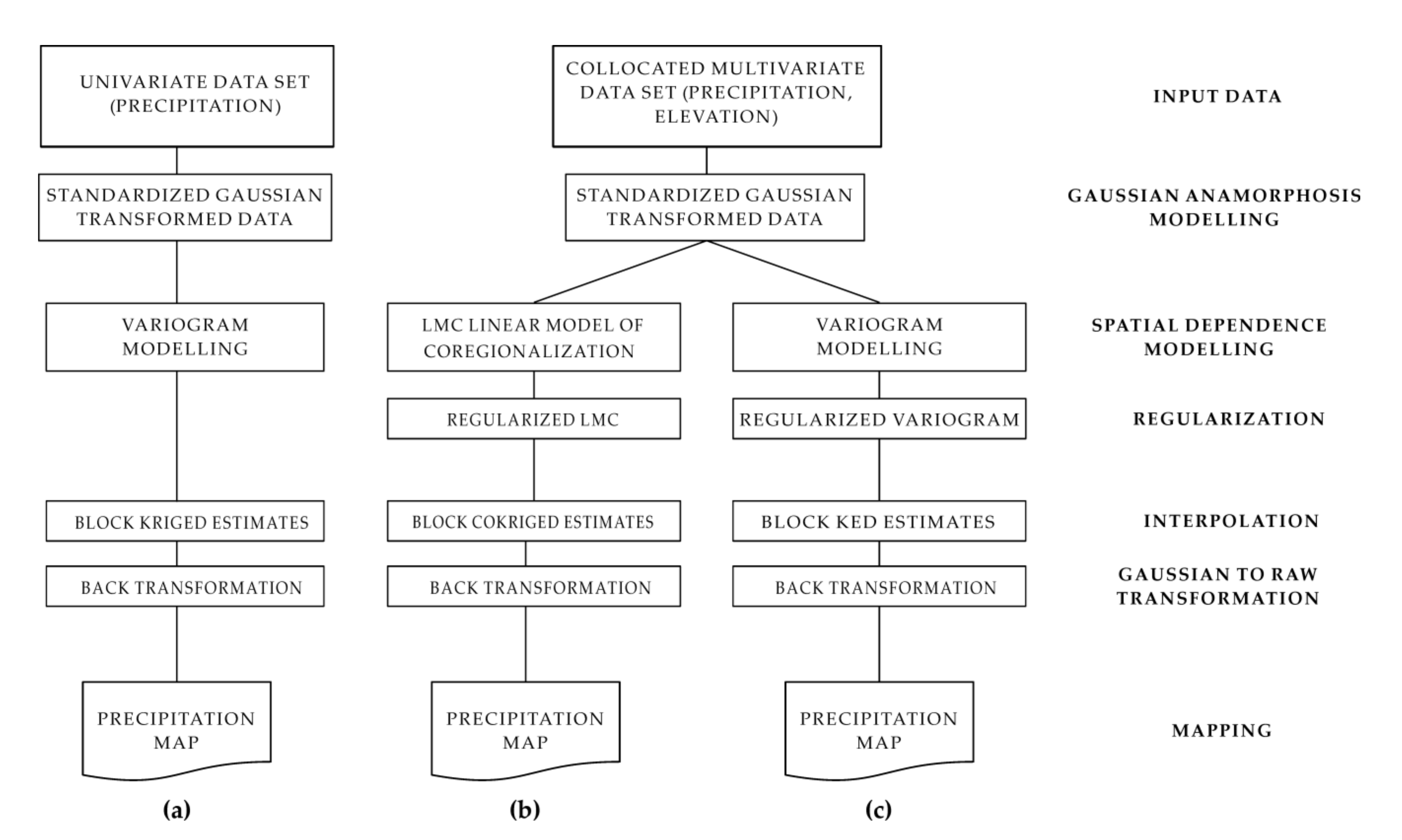
An overview of the three geostatistical approaches is shown in Figure 2.
All geostatistical analyses were performed using the software package ISATIS, release 2018.3 [45].
2.3. Validation Procedure
The whole dataset (n = 183) was randomly split into a calculation set including 146 precipitation gauge (80% of the whole dataset) and a validation set including 37 precipitation gauges (20% of the whole dataset). Figure 1 shows the locations of the calculation and validation sets. The calculation set was used both to apply the three geostatistical approaches (block ordinary kriging, block ordinary cokriging, and block kriging with external drift) following the schematic overview summarized in Figure 2 and to estimate the mean annual precipitation values at the validation set locations to provide an independent assessment of the prediction quality. Since it is unlikely that one method will produce the best estimate at all locations, the predictions were compared using three classical measures of accuracy (see for example [46,47], among others): (1) the mean absolute error (MAE), (2) the root mean squared error of prediction (RMSEP), and (3) the mean relative error (MRE). In addition, the goodness of prediction (G), as a measure of effectiveness, was calculated. The MAE is the average of the absolute residuals (e.g., predicted minus observed) [48]:
where is the number of observations in the independent validation set (here n = 37), is the estimated value at location α, and is the observed value at location α. MAE should be close to zero. The mean squared error of prediction (RMSEP) is the root of the averaged squared difference between the observed value and the estimated value ,
The RMSEP measures the precision of the prediction and it should be as small as possible. To reduce the impact of large values on the computation of the MAE, the mean relative error (MRE) has been also computed:
The fourth comparative measure is a goodness of prediction used by Agterberg [49] and is given by:
where is the sample mean. The measure G gives an indication of how effective a prediction might be, relative to that which could have been derived from using the sample mean alone [49]. If is less than , it indicates that the predictions made using are more accurate on average than those made using and G will be positive, whereas if is greater than , it indicates that the predictions made using are less accurate on average than those made using and G will be negative. The magnitude of G gives the accuracy: a value equal to 100% indicates perfect prediction.
Moreover, to analyze the effect of elevation in the validation procedure and to assure that the results were confirmed in different classes of elevation, a solution could be to split the validation set into elevation class functions representing plain, hill, and mountain. However, in order to have more or less the same number of data in the different elevation classes, it was preferred to use the quartiles of the elevation data distribution of the validation set. According to this criterion, the lower quartile, the median, and the upper quartile were used to split the data into four elevation classes, roughly ranging from lowland through hill to mountain:
- Class 1 (10 precipitation data): elevation between 3 and 120 m a.s.l.
- Class 2 (9 precipitation data): elevation between 160 and 286 m a.s.l.
- Class 3 (9 precipitation data): elevation between 304 and 498 m a.s.l.
- Class 4 (9 precipitation data): elevation between 550 and 1358 m a.s.l.
Then, the three accuracy measures (MAE, RMSEP and MRE), and the effectiveness measure (G) were calculated for the estimated precipitation values of each elevation class.
Moreover, a scatterplot of measured versus predicted values provided additional evidence on how well an estimation method has performed. The best possible estimates would match the measured values, and therefore the slope of the scatterplot should be close to 1. A good index for summarizing how close the points on a scatterplot come to falling on a straight line is the Pearson correlation coefficient. However, because highly mismatched pairs on the scatterplot influence the linear correlation coefficient, the Spearman rank correlation coefficient as measure of the strength of the relationship was also used.
Finally, as a measure of the strength of the relationship between the measured and estimates of precipitation values for each elevation class, the Pearson correlation coefficient and the Spearman rank correlation coefficient were calculated.
3. Results
The mean annual precipitation and elevation data both show asymmetric distributions (Figure 3). The distribution of the mean annual precipitation is slightly positive skewed because mean (1089.3 mm) and median (1059.8 mm) are a little different (skewness coefficient = 0.51). In addition, the upper whisker (maximum precipitation value = 2081.8 mm) is longer than the lower whisker (minimum precipitation value = 502.7 mm). Both calculation (C) and validation (V) sets for the mean annual precipitation (Figure 3) have similar means and medians.
The distribution of elevation data is moderately skewed with a more marked difference between the mean (434.5 m) and the median (367.0 m) (skewness coefficient = 0.75) than the one of precipitation data (Figure 3). The difference between the upper whisker (maximum elevation value = 1358 m) and the lower whisker (minimum elevation value = 3 m) is also greater than for the average annual precipitation. The calculation set of elevation data has a similar distribution and main statistics to the whole set, whereas the validation set has a greater asymmetry (Figure 3).
However, all data were transformed into Gaussian-shaped variables using the above-mentioned Gaussian anamorphosis. Moreover, a standardization to zero mean and unit variance is however required in a multivariate analysis when the variables are expressed in different units and have different magnitudes, as in the present study case. Therefore, all geostatistical procedures were performed in the Gaussian domain, and finally the estimates were back-transformed to the original units.
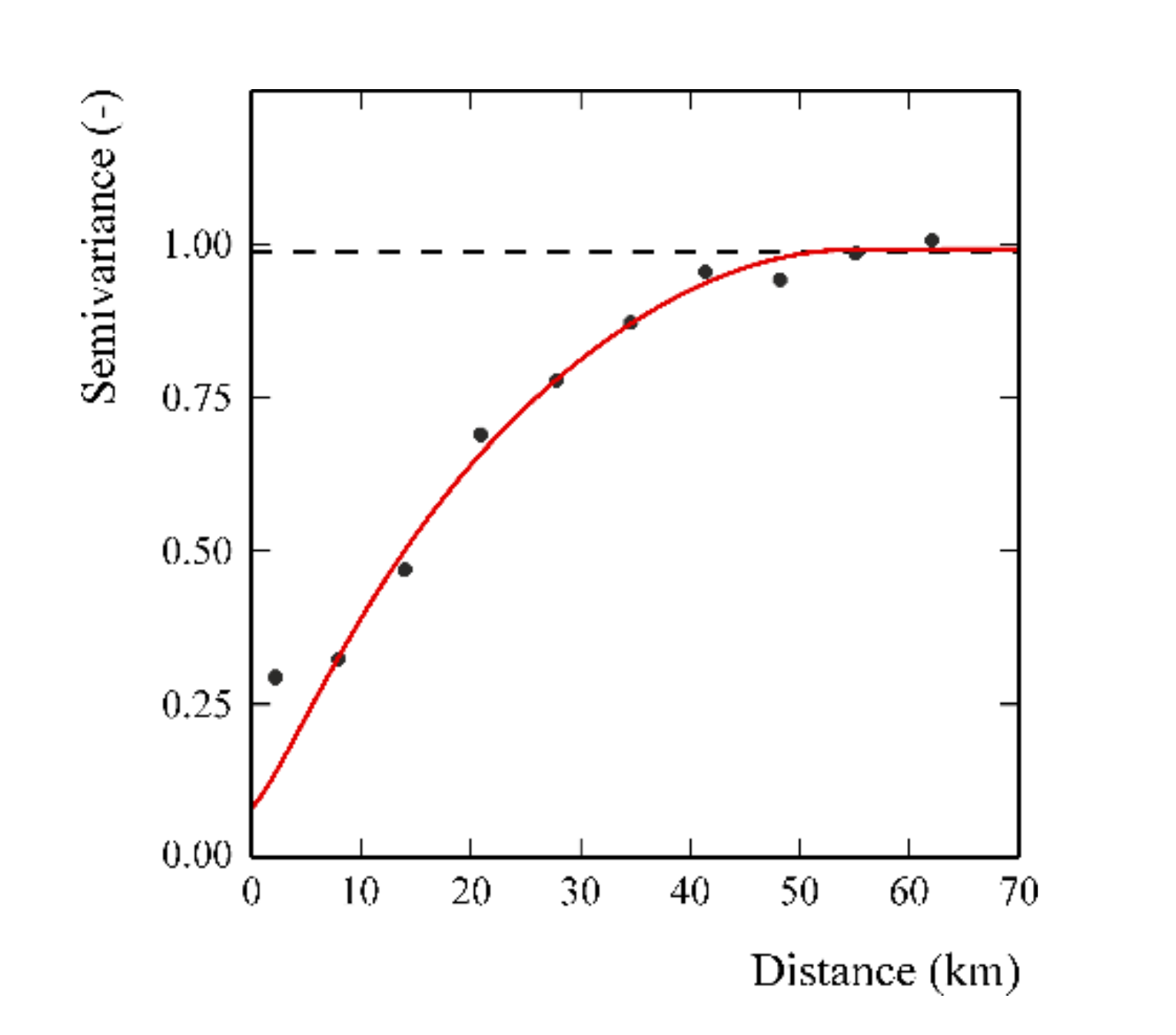
In the scope of identifying possible anisotropic behaviors, a map of the 2D variograms (not shown) of precipitation data was computed, but no relevant difference as a function of direction (anisotropy) was found. Therefore, an experimental variogram was computed and modelled by a bounded isotropic nested variogram model (Figure 4), which included three basic structures: a nugget effect, a K-Bessel model [20] with a scale (distance parameter) of about 29.8 km and a parameter equal to 1, and a spherical model [37] with range of 54.6 km.
The goodness of fit was tested through cross-validation with mean errors equal to 0.025 and a standardized error variance of 0.80. The standardized error variance is within the tolerance interval 0.7–1.3 [20].
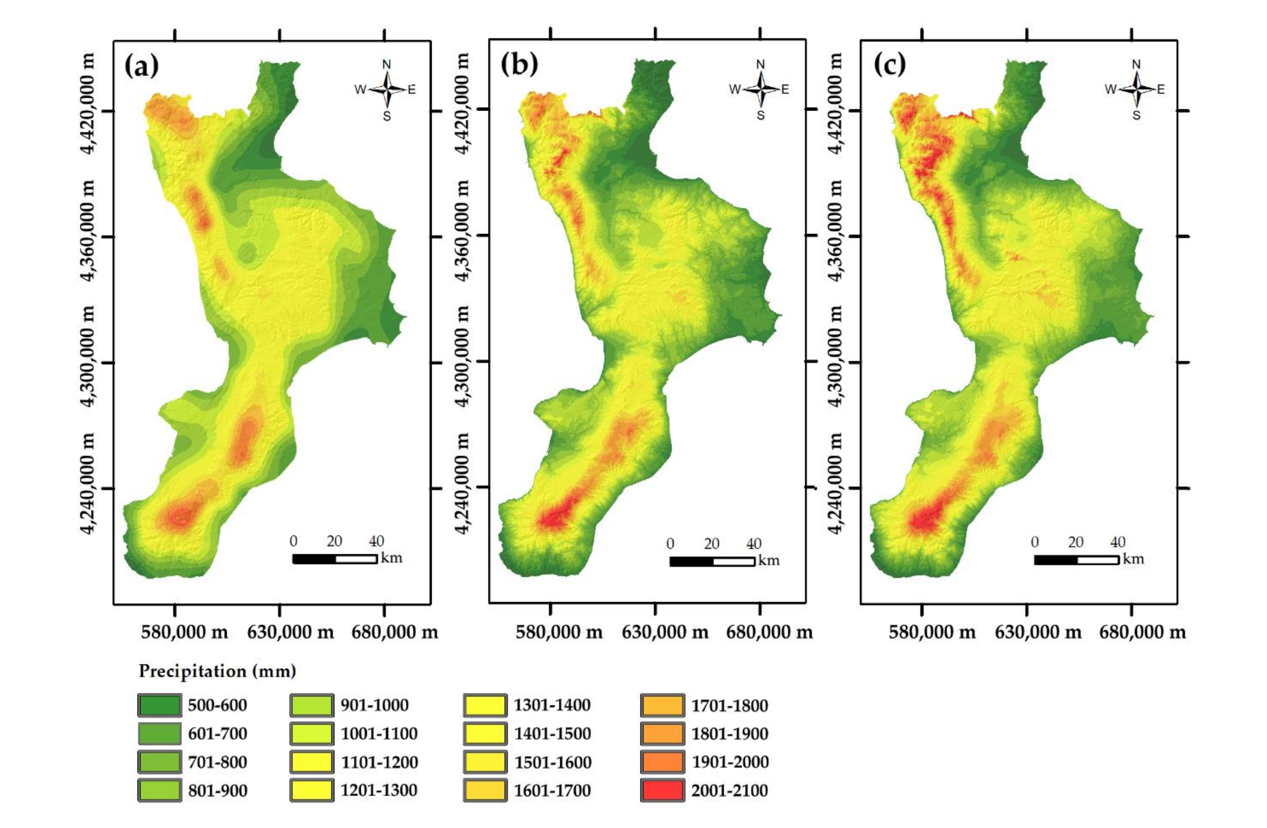
The fitted variogram and the Gaussian precipitation data were used with block ordinary kriging to estimate the values of the square blocks centered on the 80 m × 80 m grid nodes. The estimated values were back-transformed to raw precipitation using the previously determined anamorphosis function (Figure 5a).
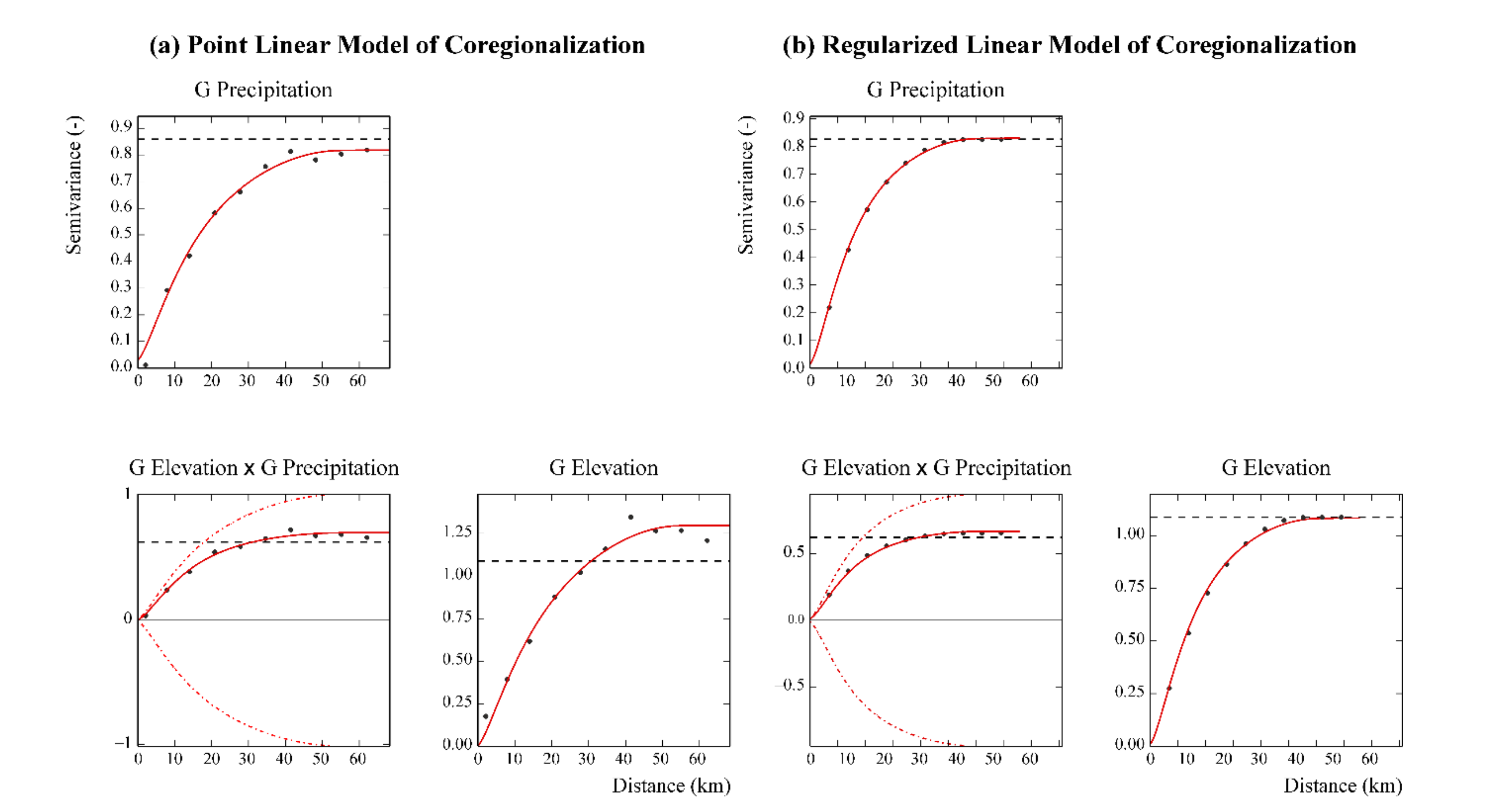
A point linear model of coregionalization (LMC) of the Gaussian-transformed variables of precipitation and elevation was computed to apply block ordinary cokriging. The LMC included three variograms (Figure 6a): one auto-variogram for each variable and one cross-variogram for the two variables.
The point LMC was fitted including the following basic structures (Figure 6a): a nugget effect, a K-Bessel model with a scale of about 29.8 km and parameter equal to 1, and a spherical model [19] with a range of about 54.6 km. The goodness of fit was tested through cross-validation with mean errors equal to 0.032 for Gaussian precipitation and 0.045 for Gaussian elevation, whereas the standardized error variances were 0.90 for Gaussian precipitation and 1.07 for Gaussian elevation. Both standardized error variances are within the tolerance interval 0.7–1.3 [20].
The experimental variograms of the Gaussian data were regularized over the 80 m × 80 m block, and the fitted block LMC included the following three basic spatial structures: a nugget effect, a K-Bessel model with a scale of about 32.4 km and parameter equal to 1, and a spherical model with a range of about 60.2 km (Figure 6b).
Finally, the Gaussian precipitation values were estimated at the square blocks centered on the 80 m × 80 m grid nodes, and then they were back-transformed to raw precipitation data using the previously determined anamorphosis function (Figure 5b).
To apply kriging with external drift, Gaussian data of elevation were used as external drift. The mean annual precipitation and elevation are linearly and positively correlated with a coefficient of 0.61 for raw data that increases to 0.66 for Gaussian values. That confirms the applicability condition of KED. The same variogram model fitted for the univariate case was used for kriging with elevation as external drift, but was regularized over the 80 m × 80 m block. Finally, at the square blocks centered on the 80 m × 80 m grid nodes, the Gaussian precipitation values were estimated and back-transformed to raw precipitation data (Figure 5c).
Finally, the calculation set was used to apply the three methods and re-estimate the precipitation values at the validation set locations. The measures of accuracy and effectiveness of the estimates obtained by the three interpolation techniques are reported in Table 1.
All measures of accuracy and effectiveness of the estimates show that block kriging with external drift (BKED) performs better than block ordinary kriging (BOK) and block ordinary cokriging (BcoK). In fact, using BKED, the three accuracy measures (MAE, RMSEP, and MRE) have the lowest values, while the effectiveness measure (G) has the highest value (Table 1).
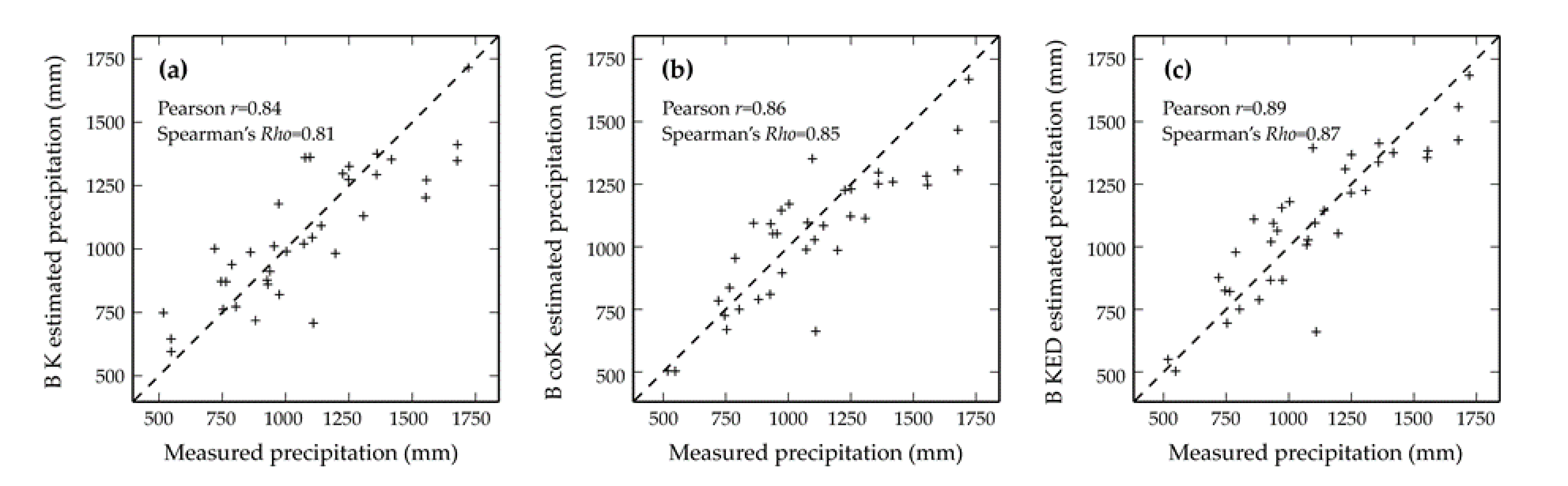
Finally, the scatterplots of estimated versus measured precipitation of the validation set (Figure 7) also show the best performance for block kriging with external drift (Figure 7c).
The largest values of the Pearson correlation coefficient r (0.89) and Spearman rank correlation coefficient Rho (0.87) for block kriging with external drift (Figure 7c) confirm the good performance of this approach.
Similarly to what was obtained from the results of the measures of accuracy and effectiveness of the estimates obtained by the three interpolation techniques, the Pearson correlation coefficient r and Spearman rank correlation coefficient Rho are higher for block kriging with external drift (BKED) than for the other methods for the validation subsets of elevation classes 2 (160–286 m a.s.l.), 3 (304–498 m a.s.l.), and 4 (550–1358 m a.s.l.), although for class 2, the Spearman rank correlation coefficient Rho of BcoK is slightly higher (0.45) than that of BKED (0.42) (Table 2).
In accordance with what happened with the measures of accuracy and effectiveness of the estimates, for the validation subset of the elevation class 1 (3–120 m a.s.l.), the Pearson correlation coefficient r and Spearman rank correlation coefficient Rho are higher for block cokriging (BcoK) than for the other methods (Table 2).
4. Discussion
As explained before, elevation and precipitation data are associated with different support sizes, which for precipitation can be considered punctual, whereas for elevation it is equal to the resolution of the digital elevation model (80 m × 80 m). Taking this difference in support into account required the regularization of variograms (Figure 6). The regularized variograms differ from the point support variograms by a constant term that measures within-block variance and is related to the size and geometry of the support [40] (Figure 6). The block LMC (Figure 6b), compared to point LMC (Figure 6a), shows that as block size increases, the sills decrease whereas the ranges increase. The nugget should also decrease because the proportion of noise in the data decreases and the nugget should be filtered. However, in this particular case, there is little apparent decrease in the nugget because it was already very small in the point LMC.
In the linear model of coregionalization of the Gaussian-transformed variables of precipitation and elevation (both point and block LMC), all variogram models (Figure 6) show a great continuity at the origin, which is an evidence of very regular processes. Moreover, the variograms also show a nested spatial structure that includes two different variogram models at short and long spatial scales. That leads to the suggestion that the variability of precipitation and elevation is due to two different processes acting at short and long range. This variability at two different spatial scales has been reported to be probably due to the orographic effect for the shorter range of spatial variation and to large-scale factors of variation as global atmospheric circulation for the longer range [7].
The visual inspection of the cross-variograms (Figure 6) allows also to check the correlation between the two variables: the proximity of the variogram model to the dotted curve (called hull) represents the maximum correlation between the two variables (intrinsic correlation) [38].
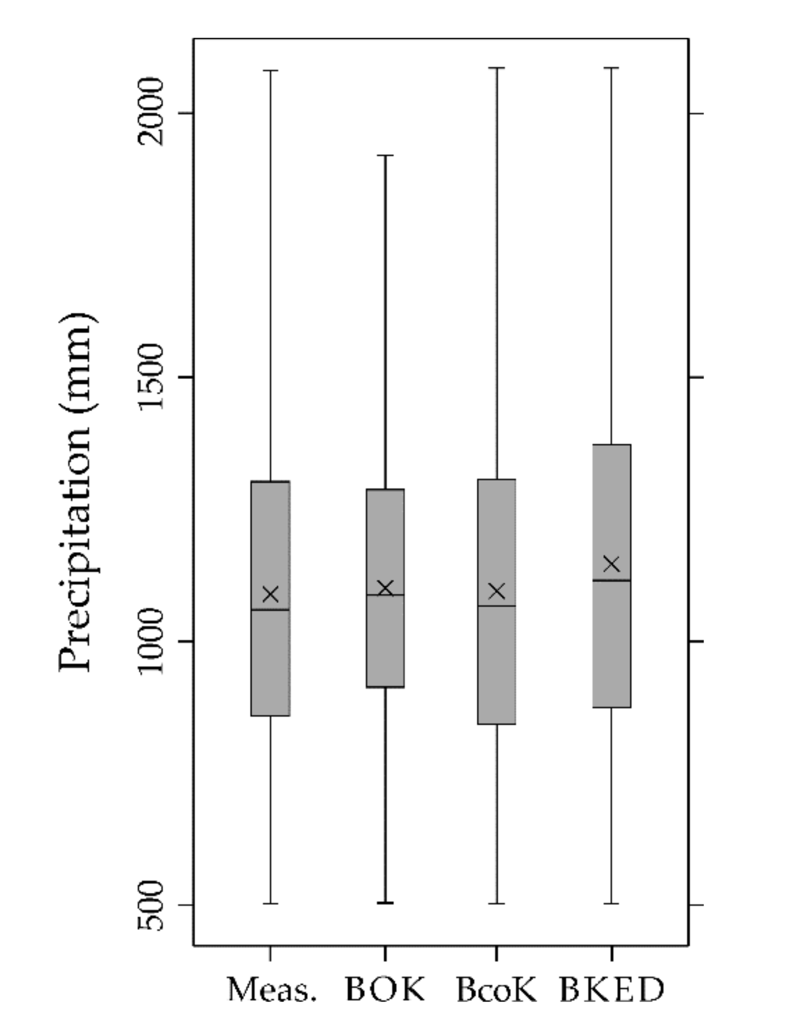
Accounting for secondary information, as in BcoK and BKED, results in maps with more details (Figure 5b,c) than that obtained by univariate block ordinary kriging (Figure 5a). Block ordinary cokriging and block kriging with external drift (Figure 5b,c) share the secondary information from elevation and their maps show similar features. It is interesting to compare the box plots of the map values obtained with the three geostatistical methods and that of the mean annual precipitation data (Figure 8).
The first thing one can observe is the smoothing effect, typical of ordinary kriging, which reduces both the interquartile range (difference between the upper and lower quartile) and the maximum value. On the contrary, both block ordinary cokriging and block kriging with external drift reproduce the statistics of the measured data better than block ordinary kriging (Figure 8).
However, Figure 5c shows that block kriging with external drift produces more local details than block ordinary kriging and block ordinary cokriging. Such “short-range” variation is due to the local re-evaluation of the linear regression of precipitation on block estimates.
These results are confirmed by other studies. For example, Lloyd [25] studied the effect of elevation on estimation of monthly precipitation in Great Britain comparing moving window regression, inverse distance weighted, ordinary kriging, simple kriging with a locally varying mean, and kriging with external drift, and has concluded that kriging with external drift provided the most accurate estimates of precipitation. In another study on the spatio-temporal analysis of daily precipitation and temperature in the Mexico basin, Carrera-Hernandez and Gaskin [50] compared OK, KED, block kriging with external drift, OK in a local neighborhood, and KED in a local neighborhood (KEDL), and the latter (KEDL), using elevation as an auxiliary variable to define the drift, performed best.
Block kriging with external drift (BKED) also clearly performs better than the other methods for the validation subsets of elevation classes 2 (160–286 m a.s.l.), 3 (304–498 m a.s.l.), and 4 (550–1358 m a.s.l.), although for class 2, the MAE of BKED (133.64 mm) is slightly higher than that of BcoK (133.12 mm). On the contrary, for the validation subset of the elevation class 1 (3–120 m a.s.l.), all measures of accuracy and effectiveness of the estimates show that block cokriging (BcoK) performs better than block ordinary kriging (BOK) and block kriging with external drift (BKED) (Table 1). However, these results clearly indicate that the use of an exhaustive secondary variable always improves the precipitation estimate. In the case of areas with elevations below 120 m, block cokriging makes better use of secondary information in precipitation estimation than block kriging with external drift. At higher elevations, however, the opposite is always true: BKED performs better than BcoK (Table 1).
5. Conclusions
The results of the study showed that block kriging with external drift, compared to block ordinary kriging and block ordinary cokriging, was the most accurate approach for modelling the spatial distribution of mean annual precipitation. The approach used elevation as external drift and took into account the support size associated with precipitation and elevation data.
However, although the results clearly indicated that the use of an exhaustive secondary variable always improves the precipitation estimate, in the case of areas with elevations below 120 m, block cokriging makes better use of secondary information in precipitation estimation than block kriging with external drift. Instead, at higher elevations, the opposite is always true: block kriging with external drift performs better than block cokriging.
The maps obtained by geostatistical approaches accounting for secondary information (such as elevation) showed to be more detailed than the one obtained by the univariate block ordinary kriging. Particularly, the maps obtained by block ordinary cokriging and block kriging with external drift, which shared the secondary information from elevation, showed similar features, but block kriging with external drift produced more local details than block ordinary cokriging because of the local re-evaluation of the linear regression of precipitation on block estimates. Moreover, both block ordinary cokriging and block kriging with external drift reproduced the statistics of the measured precipitation data better than block ordinary kriging.
The results of this study are a contribution in modelling and understanding natural processes such as precipitation at an annual time scale.
Author Contributions
G.B. conceived and designed the study, analyzed and interpreted the data, and wrote the paper; M.C. has contributed to conceive and designed the study, analyzed and interpreted the data, and wrote the paper. All authors have read and agreed to the published version of the manuscript.
Funding
This research received no external funding.
Institutional Review Board Statement
It is not relevant to our study.
Informed Consent Statement
It is not relevant to our study.
Data Availability Statement
The data used are the property of the Calabria Region and available free of charge on request. The source of the data used is clearly stated in the text.
Acknowledgments
The authors thank the reviewers for providing constructive comments, which have contributed to the improvement of the manuscript.
Conflicts of Interest
The authors declare no conflict of interest.
References
- Molden, D.; Vithanage, M.; de Fraiture, C.; Faures, J.M.; Gordon, L.; Molle, F.; Peden, D. Water Availability and Its Use in Agriculture. In Treatise on Water Science; Wilderer, P., Ed.; Elsevier Science: Amsterdam, The Netherlands, 2011; Volume 4, pp. 707–732. ISBN 978-0-44453-193-3. [Google Scholar]
- Deraisme, J.; Humbert, J.; Drogue, G.; Freslon, N. Geostatistical Interpolation of Rainfall in Mountainous Areas. In geoENV III—Geostatistics for Environmental Applications; Monestiez, P., Allard, D., Froidevaux, R., Eds.; Springer: Dordrecht, The Netherlands, 2001; pp. 57–66. [Google Scholar]
- Grimes, D.I.F.; Pardo-Igúzquiza, E. Geostatistical analysis of rainfall. Geogr. Anal. 2010, 42, 136–160. [Google Scholar] [CrossRef]
- Su, Y.; Zhao, C.; Wang, Y.; Ma, Z. Spatiotemporal variations of precipitation in China using surface gauge observations from 1961 to 2016. Atmosphere 2020, 11, 303. [Google Scholar] [CrossRef] [Green Version]
- Bostan, P.A.; Heuvelink, G.B.M.; Akyurek, S.Z. Comparison of regression and kriging techniques for mapping the average annual precipitation of Turkey. Int. J. Appl. Earth Obs. Geoinf. 2012, 19, 115–126. [Google Scholar] [CrossRef]
- Matheron, G. The Theory of Regionalized Variables and Its Applications; Ecole Nationale Superieure des Mines de Paris: Paris, France, 1971; Volume 5. [Google Scholar]
- Buttafuoco, G.; Lucà, F. Accounting for elevation and distance to the nearest coastline in geostatistical mapping of average annual precipitation. Environ. Earth Sci. 2020, 79, 11. [Google Scholar] [CrossRef]
- Lloyd, C.D. Multivariate Interpolation of Monthly Precipitation Amount in the United Kingdom; Springer: Dordrecht, The Netherlands, 2010; pp. 27–39. [Google Scholar]
- Szentimrey, T.; Bihari, Z.; Szalai, S. Comparison of Geostatistical and Meteorological Interpolation Methods (What is What?). In Spatial Interpolation for Climate Data: The Use of GIS in Climatology and Meteorology; ISTE: London, UK, 2010; pp. 45–56. ISBN 978-1-90520-970-5. [Google Scholar]
- Hengl, T.; AghaKouchak, A.; Percěc Tadić, M. Methods and data sources for spatial prediction of rainfall. In Rainfall: State of the Science; Testik, F.Y., Gebremichael, M., Eds.; American Geophysical Union: Washington, DC, USA, 2010; pp. 189–214. ISBN 978-1-11867-023-1. [Google Scholar]
- Burrough, P.; McDonnell, R.A. Principles of Geographical Information Systems; Oxford University Press: London, UK, 1998; p. 330. [Google Scholar]
- Diodato, N. The influence of topographic co-variables on the spatial variability of precipitation over small regions of complex terrain. Int. J. Climatol. 2005, 25, 351–363. [Google Scholar] [CrossRef]
- Collins, F.C.; Bolstad, P.V. A comparison of spatial interpolation techniques in temperature estimation. In Proceedings of the Third International Conference/Workshop on Integrating GIS and Environmental Modeling, Santa Fe, NM, USA, 21–25 January 1996; National Center for Geographic Information Analysis (NCGIA): Santa Barbara, NM, USA, 1996; pp. 122–134. [Google Scholar]
- Roe, G.H. Orographic precipitation. Annu. Rev. Earth Planet. Sci. 2005, 33, 645–671. [Google Scholar] [CrossRef]
- Hartkamp, D.; De Beurs, K.; Stein, A.; White, J.W. Interpolation Techniques for Climate Variables Interpolation; CIMMYT: Mexico City, Mexico, 1999; ISBN 1405-7484. [Google Scholar]
- Brunsdon, C.; McClatchey, J.; Unwin, D.J. Spatial variations in the average rainfall-altitude relationship in Great Britain: An approach using geographically weighted regression. Int. J. Climatol. 2001, 21, 455–466. [Google Scholar] [CrossRef] [Green Version]
- Kumari, M.; Singh, C.K.; Basistha, A.; Dorji, S.; Tamang, T.B. Non-stationary modelling framework for rainfall interpolation in complex terrain. Int. J. Climatol. 2017, 37, 4171–4185. [Google Scholar] [CrossRef]
- Lucà, F.; Buttafuoco, G.; Terranova, O. 2.03—GIS and Soil A2—Huang, Bo BT—Comprehensive Geographic Information Systems; Elsevier: Oxford, UK, 2018; pp. 37–50. ISBN 978-0-12-804793-4. [Google Scholar]
- Gotway, C.A.; Ferguson, R.B.; Hergert, G.W.; Peterson, T.A. Comparison of Kriging and Inverse-Distance Methods for Mapping Soil Parameters. Soil Sci. Soc. Am. J. 1996, 60, 1237–1247. [Google Scholar] [CrossRef]
- Chilès, J.-P.; Delfiner, P. Geostatistics: Modeling Spatial Uncertainty, 2nd ed.; Wiley Series in Probability and Statistics; John Wiley & Sons, Inc.: Hoboken, NJ, USA, 2012; ISBN 9781118136188. [Google Scholar]
- Dubrule, O. Comparing splines and kriging. Comput. Geosci. 1984, 10, 327–338. [Google Scholar] [CrossRef]
- Hutchinson, M.F. Interpolating mean rainfall using thin plate smoothing splines. Int. J. Geogr. Inf. Syst. 1995, 9, 385–403. [Google Scholar] [CrossRef]
- Goovaerts, P. Geostatistical approaches for incorporating elevation into the spatial interpolation of rainfall. J. Hydrol. 2000, 228, 113–129. [Google Scholar] [CrossRef]
- Hevesi, J.A.; Istok, J.D.; Flint, A.L. Precipitation Estimation in Mountainous Terrain Using Multivariate Geostatistics. Part I: Structural Analysis. J. Appl. Meteorol. 1992, 31, 661–676. [Google Scholar] [CrossRef]
- Lloyd, C.D. Assessing the effect of integrating elevation data into the estimation of monthly precipitation in Great Britain. J. Hydrol. 2005, 308, 128–150. [Google Scholar] [CrossRef]
- Berndt, C.; Rabiei, E.; Haberlandt, U. Geostatistical merging of rain gauge and radar data for high temporal resolutions and various station density scenarios. J. Hydrol. 2014, 508, 88–101. [Google Scholar] [CrossRef]
- Gabriele, S.; Chiaravalloti, F.; Procopio, A. Radar-rain-gauge rainfall estimation for hydrological applications in small catchments. Adv. Geosci. 2017, 44, 61–66. [Google Scholar] [CrossRef] [Green Version]
- Gómez-Hernández, J.J.; Cassiraga, E.F.; Guardiola-Albert, C.; Rodríguez, J.Á. Incorporating Information from a Digital Elevation Model for Improving the Areal Estimation of Rainfall. In geoENV III—Geostatistics for Environmental Applications; Monestiez, P., Allard, D., Froidevaux, R., Eds.; Springer: Dordrecht, The Netherlands, 2001; pp. 67–78. [Google Scholar]
- Martínez-Cob, A. Estimation of mean annual precipitation as affected by elevation using multivariate geostatistics. Water Resour. Manag. 1995, 9, 139–159. [Google Scholar] [CrossRef] [Green Version]
- Pardo-Igúzquiza, E. Comparison of geostatistical methods for estimating the areal average climatological rainfall mean using data on precipitation and topography. Int. J. Climatol. 1998, 18, 1031–1047. [Google Scholar] [CrossRef]
- Bárdossy, A.; Pegram, G. Interpolation of precipitation under topographic influence at different time scales. Water Resour. Res. 2013, 49, 4545–4565. [Google Scholar] [CrossRef]
- Haiden, T.; Pistotnik, G. Intensity-dependent parameterization of elevation effects in precipitation analysis. Adv. Geosci. 2009, 20, 33–38. [Google Scholar] [CrossRef] [Green Version]
- Gotway, C.A.; Young, L.J. Combining incompatible spatial data. J. Am. Stat. Assoc. 2002, 97, 632–648. [Google Scholar] [CrossRef] [Green Version]
- Goovaerts, P. Geostatistics for Natural Resources Evaluation; Oxford University Press: New York, NY, USA, 1997; ISBN 0195115384. [Google Scholar]
- Longobardi, A.; Buttafuoco, G.; Caloiero, T.; Coscarelli, R. Spatial and temporal distribution of precipitation in a Mediterranean area (southern Italy). Environ. Earth Sci. 2016, 75, 1–20. [Google Scholar] [CrossRef]
- Buttafuoco, G.; Caloiero, T.; Guagliardi, I.; Ricca, N. Drought assessment using the reconnaissance drought index (RDI) in a southern Italy region. In Proceedings of the 6th IMEKO TC19 Symposium on Environmental Instrumentation and Measurements, Reggio Calabria, Italy, 24–25 June 2016; pp. 52–55. [Google Scholar]
- Webster, R.; Oliver, M.A. Geostatistics for Environmental Scientists; Statistics in Practice; John Wiley & Sons, Ltd.: Chichester, UK, 2007; ISBN 9780470517277. [Google Scholar]
- Wackernagel, H. Multivariate Geostatistics: An Introduction with Applications; Springer: Berlin/Heidelberg, Germany, 2003; ISBN 3540441425. [Google Scholar]
- Matheron, G. Principles of geostatistics. Econ. Geol. 1963, 58, 1246–1266. [Google Scholar] [CrossRef]
- Armstrong, M. Basic Linear Geostatistics; Springer: Berlin/Heidelberg, Germany, 1998; ISBN 978-3-540-61845-4. [Google Scholar]
- Myers, D.E. Co-Kriging—New Developments. In Geostatistics for Natural Resources Characterization; Verly, G., David, M., Journel, A.G., Marechal, A., Eds.; Springer: Dordrecht, The Netherlands, 1984; pp. 295–305. ISBN 978-94-010-8157-3. [Google Scholar]
- Deutsch, C.V.; Journel, A.G. GSLIB: Geostatistical Software Library, 2nd ed.; Oxford University Press: New York, NY, USA, 1998; ISBN 0195100158. [Google Scholar]
- Gotway, C.A.; Hartford, A.H. Geostatistical methods for incorporating auxiliary information in the prediction of spatial variables. J. Agric. Biol. Environ. Stat. 1996, 1, 17–39. [Google Scholar] [CrossRef]
- Castrignanò, A.; Buttafuoco, G.; Quarto, R.; Vitti, C.; Langella, G.; Terribile, F.; Venezia, A. A combined approach of sensor data fusion and multivariate geostatistics for delineation of homogeneous zones in an agricultural field. Sensors 2017, 17, 2794. [Google Scholar] [CrossRef]
- Bleines, C.; Deraisme, J.; Geffroy, F.; Jeannée, N.; Perseval, S.; Rambert, F. Isatis Technical References; Geovariances: Avon, France, 2018. [Google Scholar]
- Yang, Y.; Zhao, C.; Sun, L.; Wei, J. Improved Aerosol Retrievals Over Complex Regions Using NPP Visible Infrared Imaging Radiometer Suite Observations. Earth Space Sci. 2019, 6, 629–645. [Google Scholar] [CrossRef]
- Yang, X.; Zhao, C.; Luo, N.; Zhao, W.; Shi, W.; Yan, X. Evaluation and Comparison of Himawari-8 L2 V1.0, V2.1 and MODIS C6.1 aerosol products over Asia and the oceania regions. Atmos. Environ. 2020, 220, 117068. [Google Scholar] [CrossRef]
- Voltz, M.; Webster, R. A comparison of kriging, cubic splines and classification for predicting soil properties from sample information. J. Soil Sci. 1990, 41, 473–490. [Google Scholar] [CrossRef]
- Agterberg, F.P. Trend Surface Analysis. In Spatial Statistics and Models; Gaile, G.L., Willmott, C.J., Eds.; Springer: Dordrecht, The Netherlands, 1984; pp. 147–171. ISBN 978-90-481-8385-2. [Google Scholar]
- Carrera-Hernández, J.J.; Gaskin, S.J. Spatio temporal analysis of daily precipitation and temperature in the Basin of Mexico. J. Hydrol. 2007, 336, 231–249. [Google Scholar] [CrossRef]
Figure 1.
Study area and precipitation gauges locations (coordinate system: Projection UTM, Zone 33N, Datum WGS84).
Figure 1.
Study area and precipitation gauges locations (coordinate system: Projection UTM, Zone 33N, Datum WGS84).

Figure 2.
A schematic overview of three approaches: (a) block ordinary kriging, (b) block ordinary cokriging, and (c) block kriging with external drift.
Figure 2.
A schematic overview of three approaches: (a) block ordinary kriging, (b) block ordinary cokriging, and (c) block kriging with external drift.

Figure 3.
Box plots of the whole (W), calculation (C), and validation (V) sets for the mean annual precipitation and elevation data.
Figure 3.
Box plots of the whole (W), calculation (C), and validation (V) sets for the mean annual precipitation and elevation data.

Figure 4.
Variogram of the Gaussian precipitation data. The filled points are the experimental semivariance values, and the red solid line is the fitted model of variogram. The black dashed line is the experimental variance.
Figure 4.
Variogram of the Gaussian precipitation data. The filled points are the experimental semivariance values, and the red solid line is the fitted model of variogram. The black dashed line is the experimental variance.

Figure 5.
Maps of the mean annual precipitation obtained using block ordinary kriging (a), block ordinary cokriging (b), and block kriging with external drift (c).
Figure 5.
Maps of the mean annual precipitation obtained using block ordinary kriging (a), block ordinary cokriging (b), and block kriging with external drift (c).

Figure 6.
Point (a) and regularized (b) auto- and cross-variograms of the Gaussian-transformed variables of precipitation and elevation. The experimental values are the plotted black points, and the red solid lines are of the model of coregionalization. The red dash-dotted lines are the hull of perfect correlation, and the black dashed lines are the experimental variances.

Figure 7.
Scatterplots of estimated versus measured precipitation for block ordinary kriging (a), block ordinary cokriging (b), and block kriging with external drift (c). The values of the Pearson correlation coefficient (r) and of the Spearman rank correlation coefficient (Rho) are also reported.
Figure 7.
Scatterplots of estimated versus measured precipitation for block ordinary kriging (a), block ordinary cokriging (b), and block kriging with external drift (c). The values of the Pearson correlation coefficient (r) and of the Spearman rank correlation coefficient (Rho) are also reported.

Figure 8.
Box plots of the measured precipitation data (Meas.) and predicted precipitation using block ordinary kriging (BOK), block ordinary cokriging (BcoK), and block kriging with external drift (BKED).
Figure 8.
Box plots of the measured precipitation data (Meas.) and predicted precipitation using block ordinary kriging (BOK), block ordinary cokriging (BcoK), and block kriging with external drift (BKED).


Table 1.
Measures of accuracy (MAE, mean absolute error; RMSEP, root-mean-squared error of prediction; MRE, mean relative error) and effectiveness (G, goodness of prediction) of the estimates obtained by the three interpolation techniques for the whole validation set and the four validation subsets. The first column in parentheses shows the number of used data for the whole set and sub-sets (Elevation classes 1, 2, 3, and 4).
| Data Set | Estimation Method | MAE (mm) | RMSEP (mm) | MRE (-) | G (-) |
|---|---|---|---|---|---|
| Whole validation set (37) | BOK 1 | 135.11 | 173.68 | 0.13 | 54.92 |
| BcoK 1 | 130.72 | 165.77 | 0.12 | 62.41 | |
| BKED 1 | 112.80 | 144.89 | 0.11 | 75.67 | |
| Elevation class 1 (10) | BOK 1 | 120.09 | 142.44 | 0.18 | 97.73 |
| BcoK 1 | 62.10 | 67.55 | 0.08 | 99.35 | |
| BKED 1 | 73.30 | 81.52 | 0.10 | 99.17 | |
| Elevation class 2 (9) | BOK 1 | 137.49 | 162.35 | 0.14 | 97.42 |
| BcoK 1 | 133.12 | 150.11 | 0.14 | 97.78 | |
| BKED 1 | 133.64 | 149.67 | 0.14 | 97.83 | |
| Elevation class 3 (9) | BOK 1 | 213.46 | 251.01 | 0.17 | 94.79 |
| BcoK 1 | 223.32 | 253.14 | 0.18 | 95.18 | |
| BKED 1 | 197.90 | 227.08 | 0.17 | 96.37 | |
| Elevation class 4 (9) | BOK 1 | 84.40 | 119.82 | 0.07 | 99.18 |
| BcoK 1 | 118.88 | 147.62 | 0.10 | 98.63 | |
| BKED 1 | 58.89 | 75.50 | 0.04 | 99.69 |
1 Block ordinary kriging (BOK), block ordinary cokriging (BcoK), and block kriging with external drift (BKED).
Table 2.
Values of Pearson correlation coefficient (r) and Spearman rank correlation coefficient (Rho) for the measured mean annual precipitation and that estimated using block ordinary kriging, block ordinary cokriging, and block kriging with external drift for the four validation subsets (Elevation classes 1, 2, 3, and 4). The first column in parentheses shows the number of used data for the subsets.
| Data Set | Estimation Method | r (-) | Rho (-) |
|---|---|---|---|
| Elevation class 1 (10) | BOK 1 | 0.89 | 0.79 |
| BcoK 1 | 0.97 | 0.89 | |
| BKED 1 | 0.96 | 0.81 | |
| Elevation class 2 (9) | BOK 1 | 0.52 | 0.57 |
| BcoK 1 | 0.42 | 0.45 | |
| BKED 1 | 0.45 | 0.42 | |
| Elevation class 3 (9) | BOK 1 | 0.74 | 0.57 |
| BcoK 1 | 0.64 | 0.52 | |
| BKED 1 | 0.72 | 0.60 | |
| Elevation class 4 (9) | BOK 1 | 0.81 | 0.58 |
| BcoK 1 | 0.86 | 0.82 | |
| BKED 1 | 0.91 | 0.90 |
1 Block ordinary kriging (BOK), block ordinary cokriging (BcoK), and block kriging with external drift (BKED).
Publisher’s Note: MDPI stays neutral with regard to jurisdictional claims in published maps and institutional affiliations. |
© 2021 by the authors. Licensee MDPI, Basel, Switzerland. This article is an open access article distributed under the terms and conditions of the Creative Commons Attribution (CC BY) license (http://creativecommons.org/licenses/by/4.0/).
Share and Cite
MDPI and ACS Style
Buttafuoco, G.; Conforti, M. Improving Mean Annual Precipitation Prediction Incorporating Elevation and Taking into Account Support Size. Water 2021, 13, 830. https://doi.org/10.3390/w13060830
AMA Style
Buttafuoco G, Conforti M. Improving Mean Annual Precipitation Prediction Incorporating Elevation and Taking into Account Support Size. Water. 2021; 13(6):830. https://doi.org/10.3390/w13060830
Chicago/Turabian StyleButtafuoco, Gabriele, and Massimo Conforti. 2021. "Improving Mean Annual Precipitation Prediction Incorporating Elevation and Taking into Account Support Size" Water 13, no. 6: 830. https://doi.org/10.3390/w13060830
Note that from the first issue of 2016, this journal uses article numbers instead of page numbers. See further details here.