
Optimal Design of District Metered Areas in a Water Distribution Network Using Coupled Self-Organizing Map and Community Structure Algorithm


Department of Civil Engineering, Kyung Hee University, 1732 Deogyeong-daero, Giheung-gu, Yongin-si, Gyeonggi-do 17104, Korea
*
Author to whom correspondence should be addressed.
Water 2021, 13(6), 836; https://doi.org/10.3390/w13060836
Submission received: 25 February 2021
/
Revised: 12 March 2021
/
Accepted: 16 March 2021
/
Published: 18 March 2021
(This article belongs to the Special Issue Risk Assessment and Decision Support in Drinking Water Systems)
Abstract
:Operation and management of a water distribution network (WDN) by district metered areas (DMAs) bring many benefits for water utilities, particularly regarding water loss control and pressure management. However, the optimal design of DMAs in a WDN is a challenging task. This paper proposes an approach for the optimal design of DMAs in the multiple-criteria decision analysis (MCDA) framework based on the outcome of a coupled model comprising a self-organizing map (SOM) and a community structure algorithm (CSA). First, the clustering principle of the SOM algorithm is applied to construct initial homologous clusters in terms of pressure and elevation. CSA is then coupled to refine the SOM-based initial clusters for the automated creation of multiscale and dynamic DMA layouts. Finally, the criteria for quantifying the performance of each DMA layout solution are assessed in the MCDA framework. Verifying the model on a hypothetical network and an actual WDN proved that it could efficiently create homologous and dynamic DMA layouts capable of adapting to water demand variability.
1. Introduction
The introduction of the divide-and-conquer paradigm in the early 1980s has simplified the computation and control of leakage in a large water distribution network (WDN) [1]. The original network is decomposed into subsectors called district metered areas (DMAs). Each DMA is separated from the remaining network via intervening valves, and flowmeters are installed to measure the water quantities entering and leaving the DMA [2]. The method for dividing a WDN into DMAs is generally called water network partitioning (WNP) and comprises two phases: clustering and sectorization [3]. The clustering phase focuses on defining the optimal configuration of the DMAs, and the sectorization phase physically decomposes the network by determining the location of flow meters and gate valves.
The operation and management (O&M) of a WDN using DMAs has been proven to have several merits, a few of which are listed as follows: (i) leakage control, which in turn reduces the quantity of non-revenue water [4,5,6]; (ii) simple pressure management [7]; (iii) prompt identification of burst pipes and speedy repair [8]; (iv) protection of the network from accidental or malicious contamination events [9,10]; (v) monitoring of water quality and optimized sensor placement [11]. By contrast, installing the DMAs in a WDN has trade-offs such as (i) increased capital cost due to device installation [12,13]; (ii) reduced pressure redundancy due to valve-controlled isolation [14]; (iii) changed water age (WA) due to altered flow paths, which may influence on the water quality in the network [15]. Thus, the balance between merits and demerits should be considered during the implementation of DMAs.
A WDN hydraulic model is a planar graph with several vertices (i.e., nodes) interconnected through edges (i.e., pipes). Therefore, a WDN inherits the attributes of most graph theorems [16]. In other words, WNP is considered to have similarities with most graph partitioning approaches and inherits their properties. Over the last decade, WNP has been considerably explored and developed [17]. Although numerous approaches have been proposed for WNP, most of them are based on graph theory and engineering judgment. Exhaustive research [18] presented state-of-the-art methodologies for optimizing the two phases of WNP.
The clustering phase is a crucial process in establishing the DMAs, as it determines the shapes and dimensions of the DMAs while minimizing the number of boundary pipes. A literature review in this field revealed the following six most commonly used approaches for water network clustering: (1) graph theory-based algorithm [19,20,21,22]; (2) traditional modularity-based algorithm [23,24,25,26,27,28]; (3) adjusted modularity-based algorithm [29,30,31,32]; (4) multilevel recursive bisection (MLRB) [3,10,13,33]; (5) spectral clustering-based method [34,35,36]; (6) multi-agent approach [37,38,39].
Several studies have been designing dynamic DMAs rather than permanent DMAs to overcome failures and enhance network reliability in abnormal cases. Giudicianni et al. [40] proposed a method to create dynamic DMAs that allow the expansion of the existing DMAs while maintaining the set of boundary pipes in each sub-area. Wright et al. [41] presented the concept of reconfigurable DMAs to enhance the service pressure, reduce leakage, and improve system resilience. Liu and Lansey [42] proposed an approach for optimal DMA design based on multiple-phase optimization. Pesantez et al. [43] developed a method to design DMAs by coupling geospatial tools (e.g., ArcGIS) and hydraulic models (e.g., EPANET). Most recently, Santonastaso et al. [44] presented a highly practical method, in which the position of existing valves in WDN was considered to adjust a generic WDN partitioning algorithm by using a dual topology matrix, resulting in feasible DMAs in reality.
In summary, many methods have been developed to divide a WDN into DMAs. However, they are classified into two general classes involving two types of computer algorithms: graph partitioning algorithms, and modularity index-based community structure algorithms. The greatest weakness of these methods is that the size and number of DMAs are fixed by the experimenter or have not been properly evaluated. This causes the WNP approaches to have certain shortcomings, listed below:
- Graph theory–based WDN partitioning, including spectral algorithms and MLRB, requires that the size and number of clusters be determined in advance [3,13,34,35,42]. Unfortunately, the optimal number of clusters (i.e., number of DMAs) is generally not known in advance. Thus, the determination of the optimal number of DMAs in a given WDN has not been addressed heretofore.
- A modularity index-based optimization approach for exploring the communities in a WDN was focused on the network topology information, whereas specific hydraulic properties of the WDN have not been considered adequately [25,26,45,46]. This means that practical engineering aspects (i.e., weighting factors of nodes/links) were not integrated/embedded into the model adequately, thus forming infeasible DMAs.
- A set of standard criteria and their degree for designing and evaluating the DMA’s performance is lacking. In reality, water utilities develop a strategy to design DMAs that focus on pressure management to ensure minimal leakage. Thus, maintaining a uniform pressure in each DMA is essential, especially in a water network with multiple sources or irregular topographical conditions. Therefore, it is desirable to propose a method that addresses these aspects.
This paper presents a novel approach for the optimal design of DMAs (i.e., number and layout of DMAs) in a given WDN. A three-phase strategy is implemented. First, the SOM and community structure algorithm (CSA) [24] are coupled to decompose a WDN into multiscale DMAs. Accordingly, an attribute matrix is constructed for training the SOM by considering the network geometry, topology, and hydraulic properties at the nodes (e.g., elevation and pressure). Thus, the SOM allows the generation of initial clusters that are homologous in terms of hydraulic properties. CSA is then coupled to refine these initial clusters to create multiscale and dynamic DMA layouts automatically. Second, a heuristic procedure based on the genetic algorithm (GA) is adopted for deciding the locations of gate valves and flow meters along the boundary pipes for realizing alternative layouts. Finally, a set of indices is proposed to evaluate the WNP performance of the alternative solutions. Five indexes, i.e., demand similarity, pressure similarity, resilience, WA, and capital costs, are considered to assess the performances of the WNPs. To this end, a multiple-criteria decision analysis (MCDA) framework using the technique for order preference by similarity to ideal solution (TOPSIS) [49] is employed to determine the optimal design of DMAs in the network.
2. Methods
2.1. Characteristics of WDN
From a topological point of view, the structures of a WDN are modeled as a graph and are represented using a matrix [50]. The following sections present the mathematical structure and basic properties of a WDN using several matrices.
2.1.1. Adjacency Matrix
A WDN is presented mathematically by mapping onto a graph , where is the vertex set of nodes representing the junctions, reservoirs, and tanks, and is the set of edges containing pipes, valves, and pumps. The adjacency matrix is the most common representation of a graph, which indicates the vertices to which a given vertex is adjacent. The adjacency matrix of an undirected network is square and symmetric. Considering a pair of nodes and has elements , defined such that
The degree of a node (DoN), , reflects the number of edges connected to a vertex and is defined as
The adjacency matrix is a fundamental technique used in mathematics for representing and solving graphs. In the subsequent sections, advanced matrices are described based on the adjacency matrix to measure the strength of the relationship between pairs of nodes in the network.
2.1.2. Topology Similarity (TS) Matrix
The topology similarity (TS) index is used to quantify the closeness between node degrees in a network [51]. In terms of the topology, the nodes in a pair are similar if they share several neighbors. For a pair of nodes and , let and denote the set of neighbors of nodes and , respectively. According to Salton et al. [52], the TS is defined as the number of common neighbors of two nodes divided by the geometric mean of their DoNs:
where is the topology similarity index of nodes and , and its value is bounded between 0 and 1. A higher value indicates that two nodes are likely to be grouped into the same cluster.
2.1.3. Hydraulic Similarity (HS) Matrix
The hydraulic similarity (HS) index is used to quantify the correlation between a pair of nodes in a WDN based on its elevation and pressure. Consider a pair of nodes and . They are similar in terms of hydraulics if the root-mean-square deviation (RMSD) of the elevation and pressure is the lowest; in other words, the RMSD subtraction from 1 gives the highest value. Nevertheless, distinguishing the linkage between a pair of nodes as directly or indirectly connected may result in inaccurate identification of the network’s clustering structure. Thus, the HS between a pair of nodes is formulated as follows:
where and are the differences in elevation and pressure between nodes and . They can be calculated by normalizing two data measurements, in which
and
where and , and and are the elevations and pressures at nodes and , respectively. and are the maximum elevation and pressure among all nodes in the network, respectively. The value of the HS index in Equation (4) ranges between 0 and 1; a higher value indicates greater similarity between nodes in a pair in terms of hydraulics.
A DMA is formed by a set of nodes with the maximum similarity. In other words, a DMA configuration should guarantee the following:
- The pairs of nodes in the DMA have a high TS index and HS index;
- The pairs of nodes within a DMA must be connected directly.
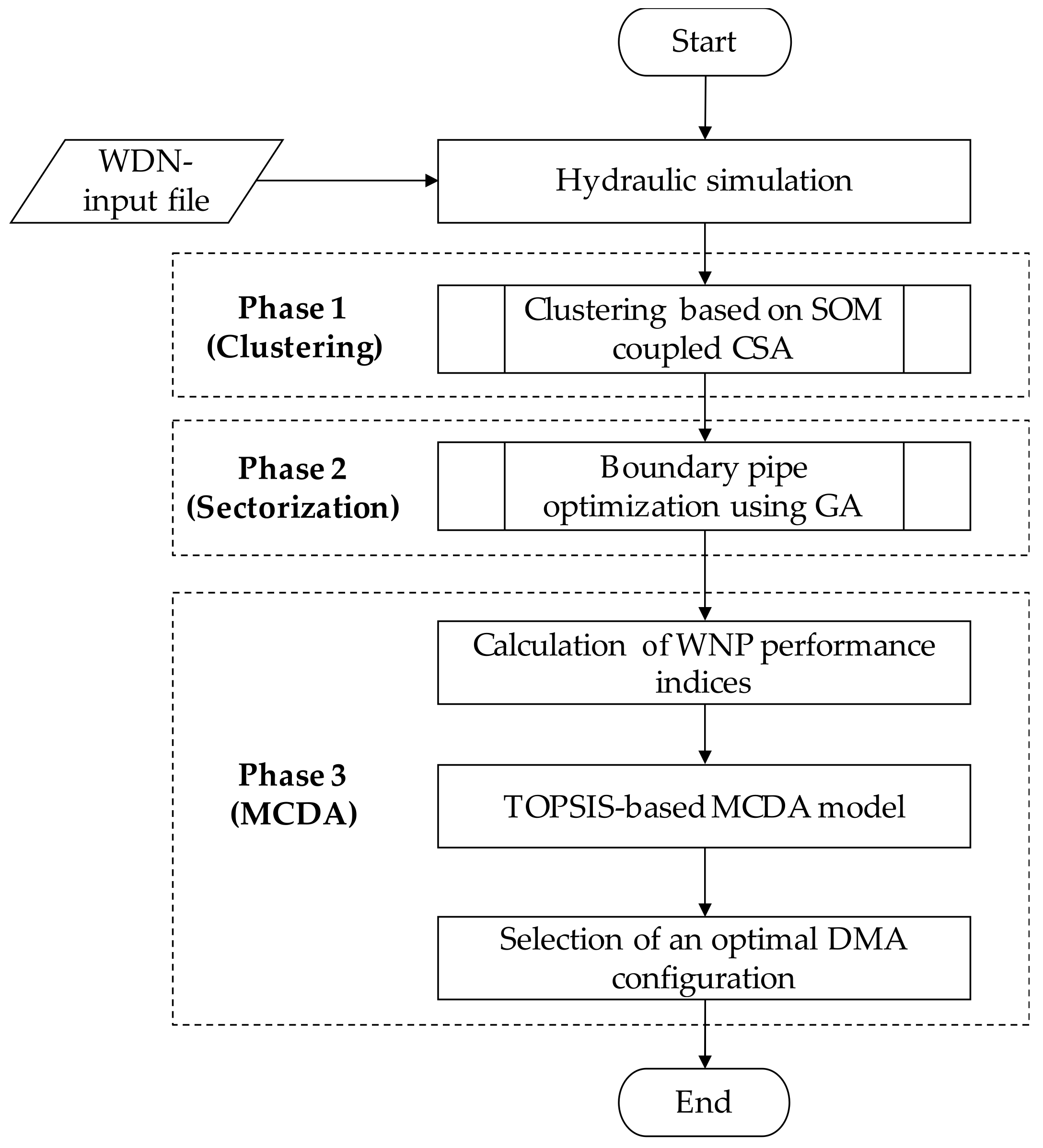
Figure 1 shows the flowchart of three main phases of the proposed method:
- In the clustering phase, hydraulic and topological data are prepared. Then, SOM is adopted to form homologous clusters before the CSA is applied for refining cluster sizes into multiscale DMAs;
- In the sectorization phase, flowmeters and gate valves are optimally located in the boundary pipes identified in the clustering phase;
- In the MCDA phase, TOPSIS is designed to rigorously evaluate the performance of the multiscale DMA layouts that are obtained in the sectorization phase, aiming to determine the optimal DMA layout in a given WDN. The detailed methodology proposed for each phase is described in the following sections.
2.2. Phase 1: Coupled Model of SOM and CSA for Clustering Dynamic DMAs
2.2.1. SOM-Based Clustering of Homologous Regions in WDN
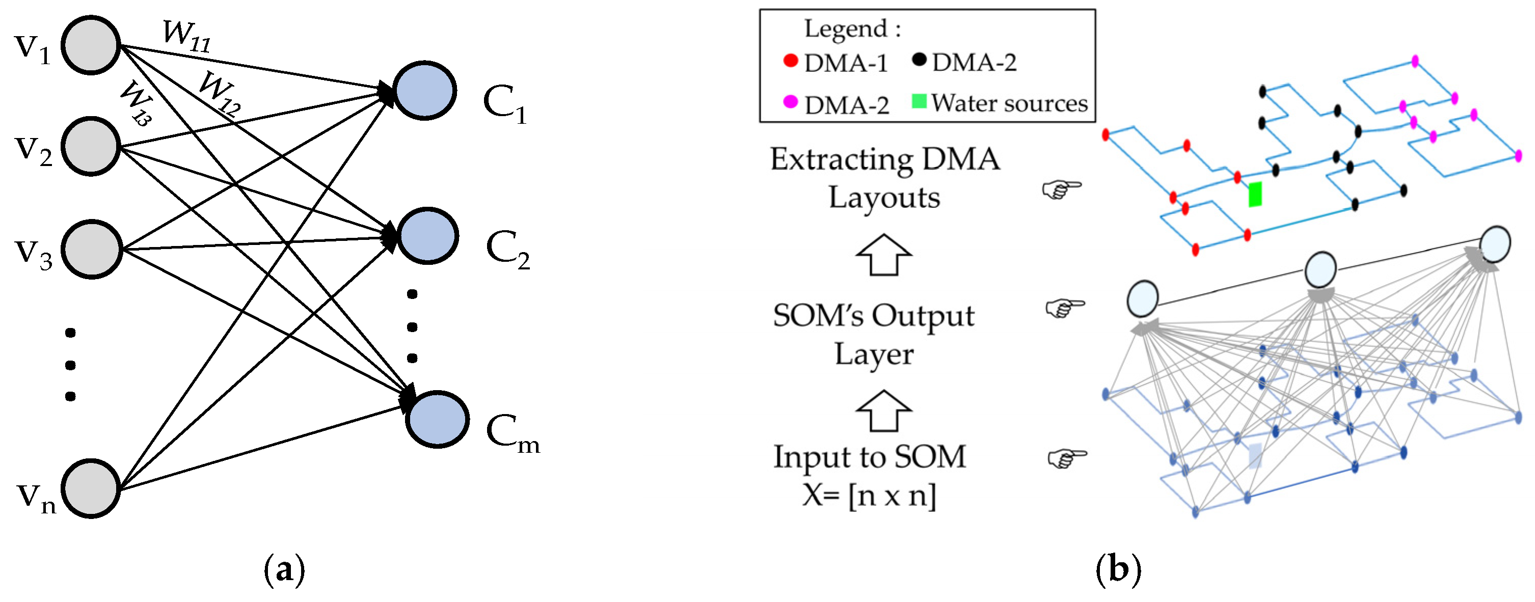
The SOM is a specific type of ANN method developed by Kohonen [47]. A SOM is an unsupervised clustering method that can learn/classify patterns from data without external supervision. The original purpose of the SOM is to transform high-dimensional input data into lower-dimensional data (generally two dimensions), thus making it easier to analyze and visualize the topology of the input data. The main advantage of the SOM is that it preserves the topology of the input data structure after training, thus revealing the optimal number of clusters inherent to the input space by mapping it to a two-dimensional structure. The structure of the SOM model is illustrated in Figure 2a. An in-depth discussion of the SOM algorithm can be found in the literature [47,53]. A brief description of the SOM model for clustering a WDN into homologous regions is provided subsequently.
As seen in Figure 2a, a SOM contains a single layer of neurons ( directly connected to -dimensional input vectors ( by random weights (. Here, the length of an input vector is equal to the number of nodes in a given WDN. As discussed in Section 2.1, the topological and hydraulic relationship between pairs of nodes in a WDN is represented by a matrix () given as
where A, TS, and HS are the adjacency matrix, matrix, and matrix, respectively. To visualize the formulation, Equation (7) can be rewritten as
where is the number of nodes in the network, is a symmetric matrix, and , for . Thus, the SOM input vector is equivalent to each column of matrix (i.e., ) and the larger the value of its element is, the more possible that nodes and will be in the same cluster. To eliminate the sensitivity of the scale variation, the input values are normalized before training the SOM.
The neurons of SOM (i.e., output layers) are generally arranged in a typical two-dimensional structure. Higher-dimensional output layers are also possible but are generally not encouraged because it is difficult to visualize layers with more than three dimensions. In the SOM architecture, each neuron is a black box where a mathematical operation is executed during the training time and reveals the topological structure of the input space. The SOM size has a significant effect on the degree of stratification of the input space. A small SOM size may aggregate much of the input’s spatial structure, whereas a large size would result in many different strata. Hence, in this study, the output layer’s size was determined by a self-adaptive approach based on the scale of variation of pattern values at the nodes in Equation (8) to ensure that the maximum possible number of clusters is formed from the input data. Figure 2b illustrates the utilization of a trained SOM for a hypothetical WDN with a map size of .
The weight vector of each neuron has the same dimension as the input pattern. It is denoted by the following equation:
where is the weight vector that connects the th neuron to the th input layer; is the number of neurons in the output layer, and is the total training nodes in the WDN.
The training process begins with all weights initialized randomly based on the principal components of the input data. Then, the SOM model calculates the similarity between each input vector and the weight vector . The Euclidean distance is used to measure the closeness between and as follows:
where represents the Euclidean norm. A smaller similarity value of indicates that the two vectors are very similar. Thus, the output neuron with the weight vector that has the smallest similarity is taken as the winning neuron.
The weight vector of the winning neuron, as well as those within a certain radius of the winning neuron, are adjusted and updated. The adjusted weight of the winning neuron is given as follows:
where and are parameters of learning rate and topological neighborhood (i.e., neighborhood radius), respectively. Hence, the updating weight vector at the time is defined by the equation as follows:
where and are learning rate parameters and neighborhood radius at time , respectively. Equations (11)–(13) are repeated sequentially for all neurons in the output layer and cycled through until the weight vectors converge within a certain tolerance or the defined number of iterations is reached.
In Equations (12) and (13), the learning rate is a parameter that reflects the contribution of each training input vector to the updated weight of the vector. It has a value between 0 and 1 and is updated during the training time as
where is the number of nodes in the WDN. The neighborhood radius () is a parameter that influences the search of the neighboring winner neurons. The higher the value of , the more strongly the neurons are affected by the weight update of an individual neuron in each training step. In this study, the Gaussian neighborhood function is used to determine the radius of influence of the winner neurons.
2.2.2. CSA-Based Creation of Multiscale and Dynamic DMAs
An advanced tool for visualizing the clustering results from SOM is the U-matrix. In U-matrix, each neuron maps the average Euclidean distance between each input node and its nearest neighbors in a high-dimensional space onto the two-dimensional map within the grids of the U-matrix. In other words, the neurons are the place to archive input nodes and their neighbors with the closest similarities. Therefore, after the SOM training, the neurons are considered initial clusters, and the potential number of homologous regions is revealed.
On the other hand, because the input data is a high-dimensional space (i.e., matrix, where is the number of nodes in the WDN) and contains various data patterns (e.g., the variations in the topological and hydraulic values at the nodes), the visualization of the cluster regions using the U-matrix may not be clear. Neurons in the SOM’s output structure are then mapped on a real WDN being considered. By doing so, it is possible to examine whether a node is assigned to a cluster while being physically outside of this cluster. Therefore, the initial clusters may larger than the number of neurons in the SOM structure, leading to a coarser and unbalanced layout (e.g., size and number of clusters). This means that the initial clusters from the SOM model need refinement to reduce the number of groups, increase the quality of clustering, and balance the number of nodes allocated to each cluster to create practical DMAs in reality.
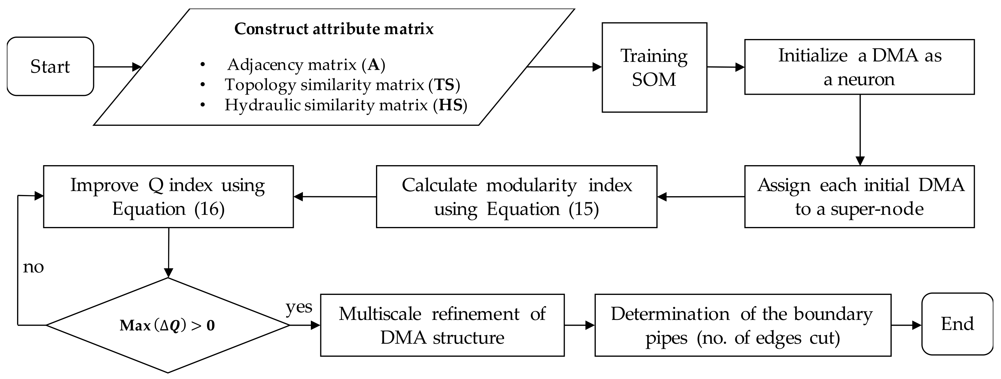
For these reasons, the CSA is embedded as an external method to evaluate and strengthen the quality of clustering implemented via the SOM. After the initial clusters have been attained from the SOM model, they are reconstructed into new clusters. All initial clusters are compressed into a super-node that connects each other by external links (i.e., links connecting boundary nodes in different clusters). The modularity-based CSA proposed by Clauset et al. [24] is used to calculate the modularity index as follows:
where is one-half the fraction of links that join the nodes in cluster to those in cluster . Thus, is the total fraction of links that occur within the clusters, and is the fraction of all the ends of links that are joined to the nodes in the cluster .
The change in upon joining of two neighboring clusters and , whether make an increasing or decreasing as follows:
In each step, the algorithm searches for the maximum among the positive values of and joins that corresponding pair of clusters to achieve the highest increase in modularity. For this CSA, the modularity index is updated by adding to the previous step. At the end of the iteration process, the number of communities decreases by 1.
By adopting this approach, the CSA performs two functions. The first is the automated creation of multiscale DMAs by merging the clusters into new bigger clusters based on the modularity index. The second is dynamic partitioning; thus, the DMAs obtained are dynamic configurations. In particular, the new layout reconfiguration obtained after the size-reducing multiscale DMAs in the present step always preserves the set of boundary pipes in the previous steps [40]. In other words, a set of boundary pipes for any new DMA layout always maintains a subset of the previous layout. Using the coupled model of SOM and CSA allows to dynamically aggregate/disaggregate network to multiscale DMAs while taking advantage of homologous clustering created by SOM. Whilst, the use of CSA alone for clustering mainly focuses on modularity index, which is the quality measure of network density to define the clusters with assuming that the density of a network division is effective if there are many edges within communities and only a few between them [24,25].
The flowchart in Figure 3 summarizes the procedure to develop the initial clusters into multiscale and dynamic DMAs in the proposed method:
2.3. Phase 2: GA-Based Sectorization
The shape and size of each DMA were determined in the clustering phase, which means a set of boundary pipes was identified. This second phase, called sectorization, aims to determine the location of flow meters and gate valves among the boundary pipes to decompose the network into independent DMAs.
A minimum number of flow meters should be installed to reduce the initial investment budget and operating costs from the O&M perspective. In contrast, a greater number of closed gate valves results in increased head loss and internal power dissipation. Thus, it reduces resilience against the occurrence of a failure in the system. In essence, an optimization process can be implemented to achieve several user-oriented goals. Laucelli et al. [4] proposed a method that simultaneously considers three objective functions for optimal DMA segmentation, such as minimizing the number of flow meters and intermitting customer demand while maximizing the reduction of leakage. Zhang et al. [45] presented a framework to locate devices by minimizing the number of boundary pipes and maximizing network pressure and WA uniformity. Campbell et al. [54] optimized the sectorization tasks by integrating a series of energy, operation, and economic criteria. Recently, Giudicianni et al. [40] developed a heuristic framework for dynamic partitioning of WDNs using multi-objective functions to address different goals for saving energy, water, and cost. Similarly, various objective functions have also been reported in [29,30,42].
The objective functions for sectorization essentially vary among designers and depend on the final goal of the WNP. Regarding energy, the total power of a WDN is categorized into dissipated power at the pipes (i.e., internal power loss) and supplied power at the node (i.e., external power supplied). In this study, the optimal position of gate valves aims to maximize supplied power at the nodes. A heuristic procedure using the GA was developed to maintain the hydraulic performance of the network at the lowest dissipated power. This requires maximizing the nodal head after sectorization. It is formulated as the following objective function:
where is the specific weight of water, and and are the elevation, pressure, and water flow at node under peak demand conditions, respectively.
Nevertheless, the objective function is constrained by the expression of Equation (18) to ensure that all nodal pressures must be equal or higher than the minimum required pressure to serve all users.
where is the minimum nodal pressure in a network and is the minimum required pressure. It varies among the countries/cities or according to the capability of the water utilities. In addition, the maximum number of flowmeters is constrained to be less than or equal to the number of DMAs in the network.
The GA is implemented as follows: each individual in the population set is a solution represented by a sequence of binary chromosomes with a length equal to the number of boundary pipes (. At the boundary pipes, either a flowmeter or gate valve is installed. Thus, the number of flowmeters ( to be installed in the network is chosen, then
in which corresponds to the number of gate valves to isolate the DMAs. Therefore, the chromosome corresponding to the th boundary pipe is set to 0 if a gate valve is installed or to 1 if a flow meter is installed [3,34,40]. Each individual is evaluated by computing the fitness value Equation (17) to choose the optimal solution.
2.4. Sample Network Demonstration of Phases 1 and 2
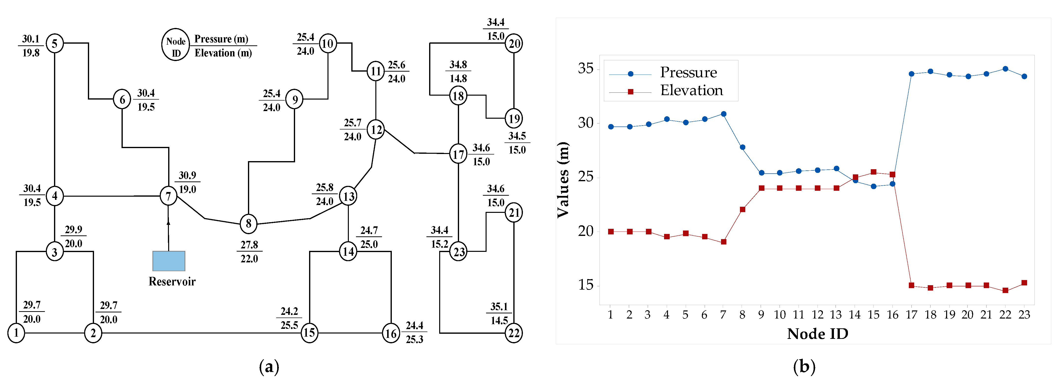
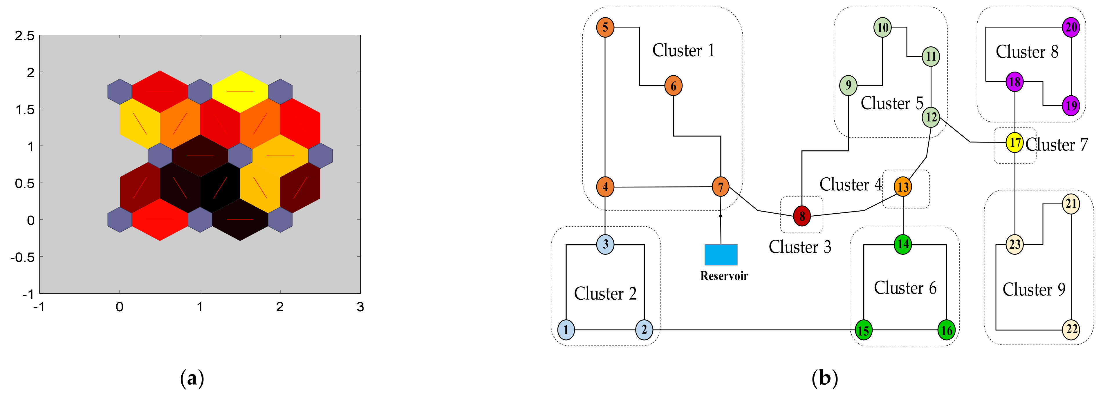
A sample WDN with 23 nodes and 28 pipes is presented here to illustrate the proposed method. The layout of the network and hydraulic properties are shown in Figure 4a. The elevation and pressure changes at the nodes dividing the network into three distinct regions can be seen in Figure 4b.
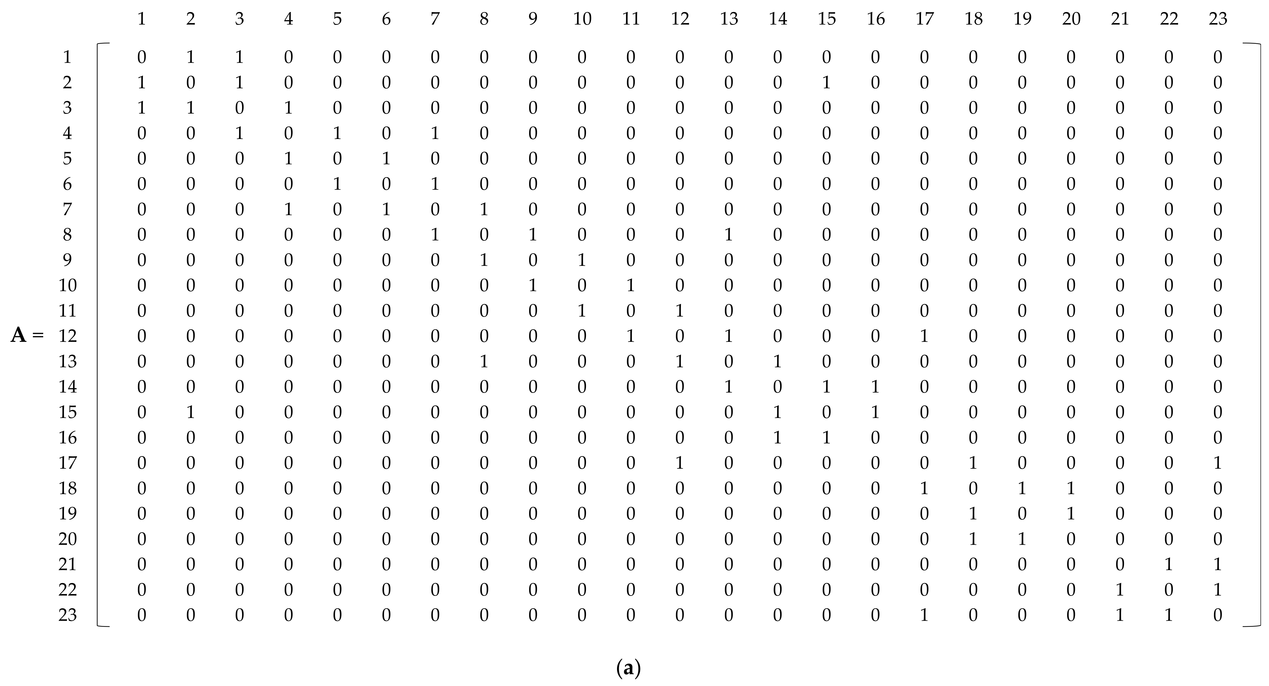
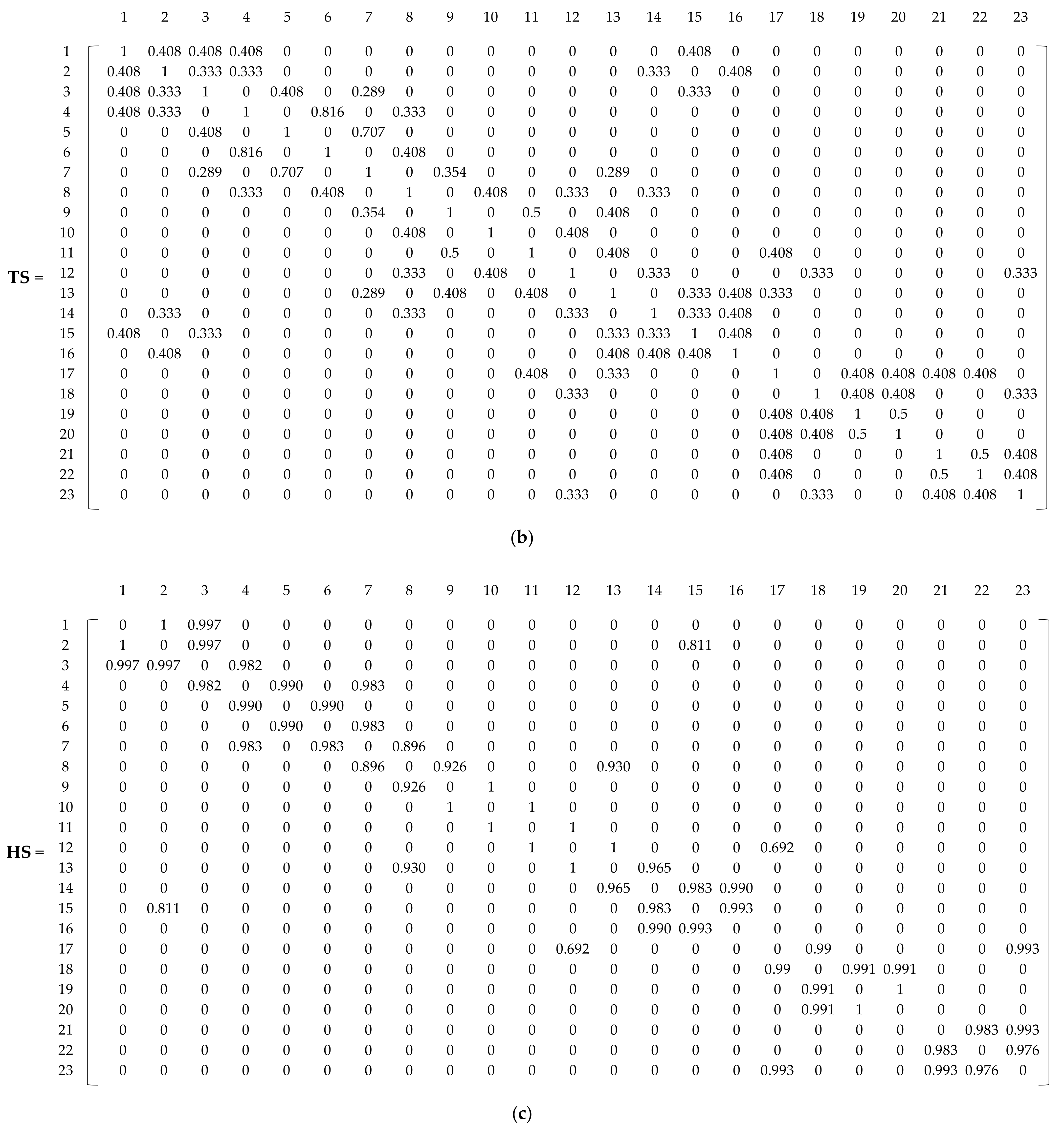
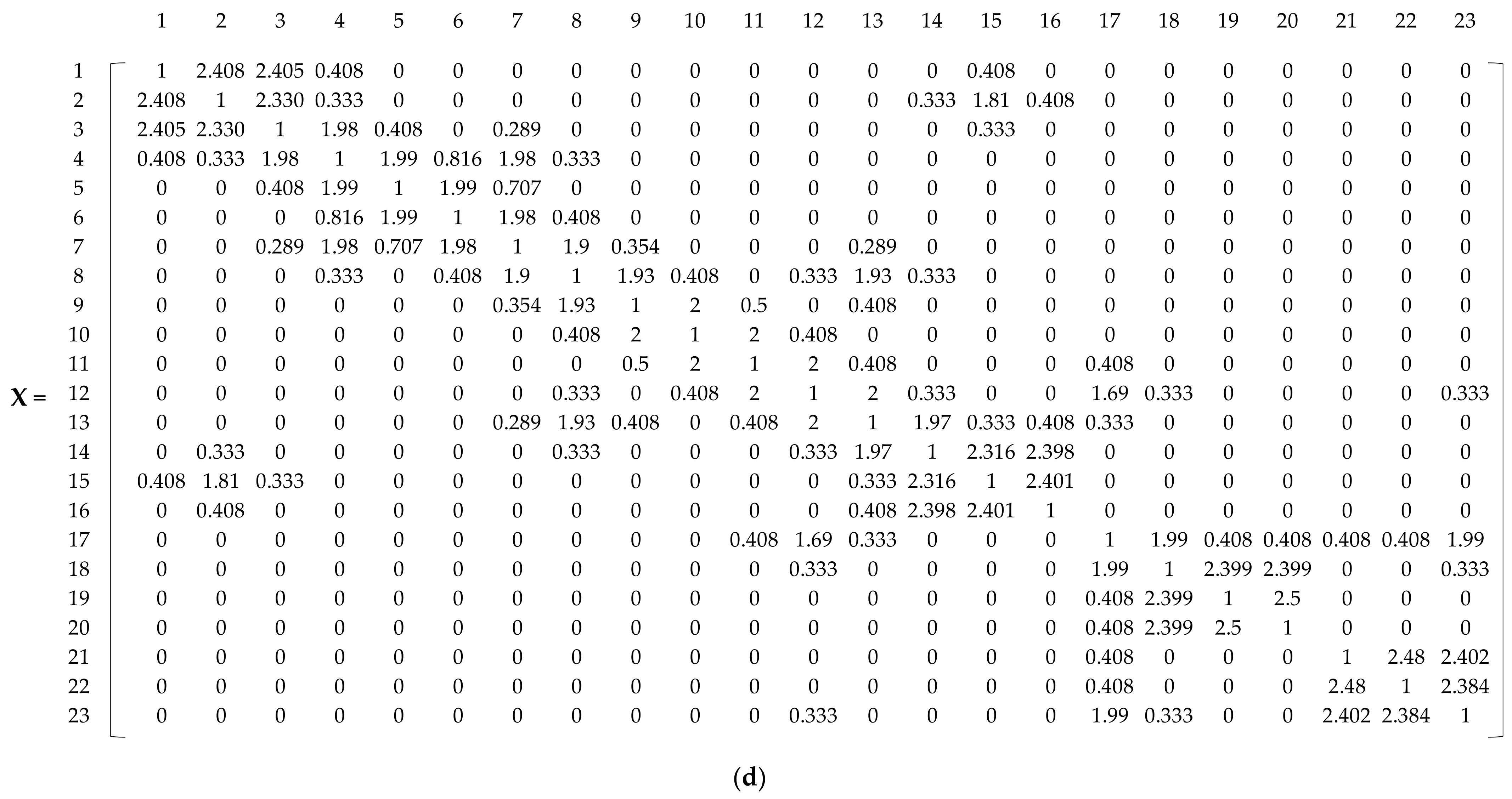
The network is abstracted to the A matrix, TS matrix, and HS matrix obtained based on Equations (1), (3), and (4), respectively, and they are sequentially reported as three matrices as shown in Figure 5a–c. The TS matrix is described by Equation (3) and quantifies the topological similarity of a pair of nodes. According to Equation (4), the HS matrix illustrates the correlation between the elevations and head pressures of a pair of nodes. Before normalization for training the SOM, an integrated matrix created by adding up the three attribute matrices of A, TS, and HS was obtained based on Equation (7) as shown in Figure 5d.
The pairs of nodes with the most similar values are grouped into a cluster. Therefore, based on each column of the matrix, node 1 has a greater tendency to connect with nodes 2 and 3 to form a cluster, whereas nodes 4 and 15 are less likely to group with node 1. Similarly, node 2 has a greater possibility to match nodes 1 and 3, followed by node 15. In contrast, node 2 is less likely to be connected with nodes 4, 14, and 16.
For the sake of simplicity, SOM is applied and expressed according to the following processes. Because of the differences in the scales of the values in the input matrix (), normalization is conducted to reduce the sensitivity before training the SOM. The SOM input here is a 23 × 23 symmetric matrix (equal to the number of nodes in the WDN). Based on the size of the training dataset, the SOM was arranged and visualized on the two-dimensional grid map comprising 3 × 3 cells (i.e., nine neurons). After a total of 50,000 iterations, the initial DMA was created. It was visualized as a U-matrix of the SOM, as shown in Figure 6a, and the nodes belonging to these DMAs were labeled as shown in Figure 6b.
In the visualization results in Figure 6a, the nine neurons represented by blue hexagons are fully connected in a mesh with multicolor regions to indicate the distance between two neurons. The neurons connected by hexagons of lighter colors indicate a small distance between each other. The darker the color, the greater is the distance between the neurons. Although the configuration and number of clusters are empirically determined based on the U-matrix, it is difficult to visualize because different colors’ strata are unclear. To produce a clustering structure more visible, the SOM sample hits where the number of input items matched to each neuron is mapped onto a two-dimensional plane. The configuration in Figure 6b exposes nine initial clusters equivalent to the nine neurons in the U-matrix; specifically, it reveals the nodes that are grouped into the same clusters. As shown in Figure 6b, clusters 1, 2, 5, 6, 8, and 9 are generated by assembling the neighbor nodes, thus creating homologous clusters. In other words, the nodes in each cluster are very similar to each other in terms of the topology and hydraulic indices. Clusters 3, 4, and 7 include only one node. This means that the nodes in these clusters are not homologous with the remaining nodes in the network (i.e., heterogeneity in terms of elevation and pressure, which does not allow the grouping of these nodes with the neighboring clusters). In short, the SOM shows high performance in the detection of homologous clusters and outlier clusters in the WDNs.
Because an initial macro DMA is generated and its size is unbalanced, it is not feasible yet for O&M. Thus, the CSA proposed by Clauset et al. [24] is applied for two reasons. First, CSA allows the detection of the dynamic DMA configuration by rescaling the initial DMAs to obtain a new, larger DMA, in which a set of boundary pipes is a subset of the initial layouts. Thus, it balances the size of the DMA and reduces the computational burden on the subsequent sectorization phase. Second, using the results from the SOM, the CSA will effectively reduce the running time to obtain a final DMA aggregation in a complex network [55].
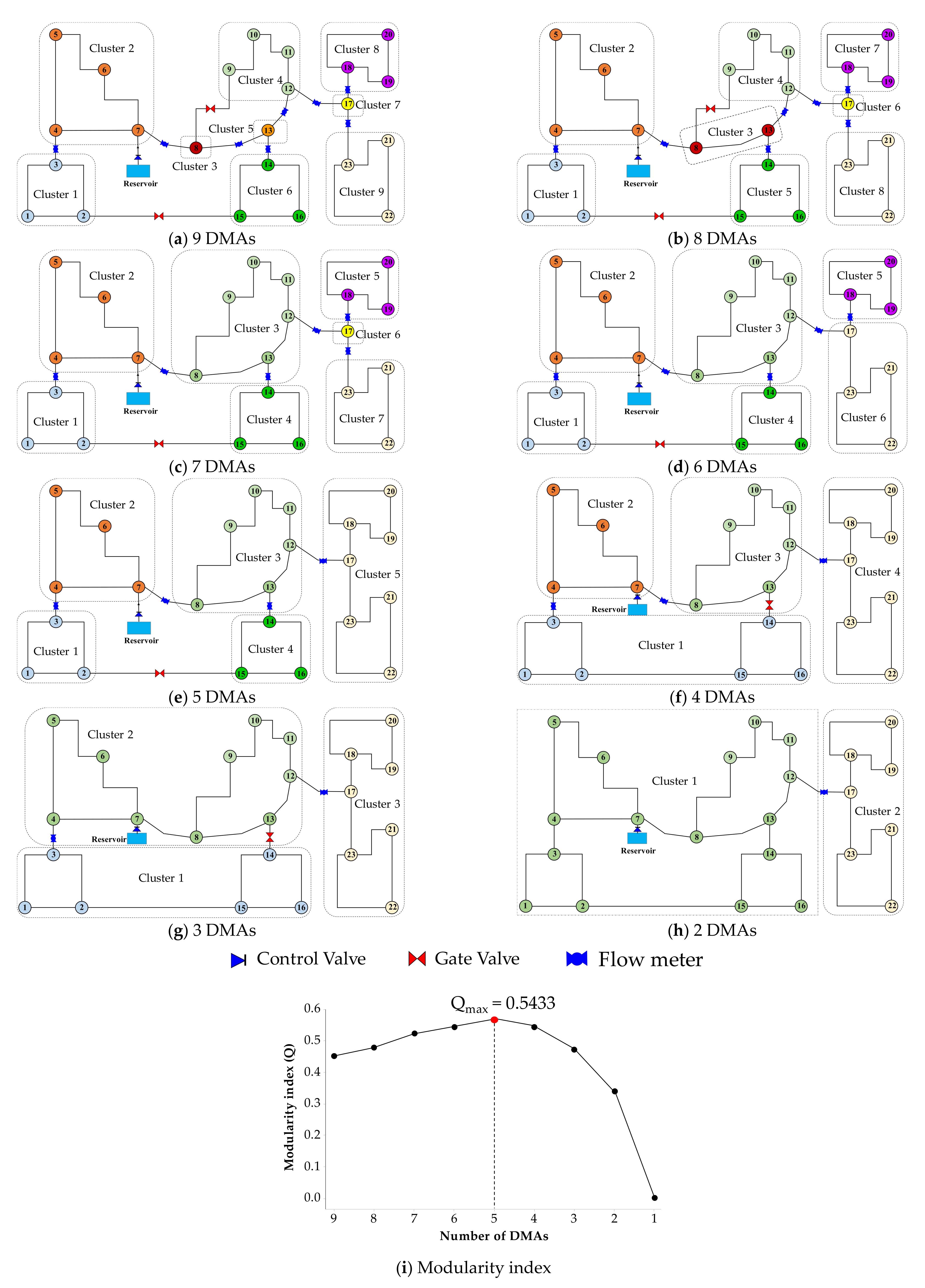
The CSA qualifies the communities in a network based on the modularity index (); thus, the possible number of DMAs is determined using . As a rule of thumb, a DMA layout is acceptable if the index is greater than 0.3 [55]. Figure 7a–h illustrates the change in the DMA layout configuration by implementing the CSA, and Figure 7i shows the variation in depending on the number of DMAs.
A variance measurement was introduced to verify the results observed in the clustering phase. It indicates how far the nodal pressure deviates among the nodes in comparison with the mean within the same cluster.
where is the number of nodes in the cluster , and and are the pressure at the node and the average pressure of all nodes in the cluster , respectively.
Table 1 lists the variance of the pressure in each cluster for multiscale layouts, as shown in Figure 7a–h. As can be seen, the SOM results for nine clusters create uniform clusters in terms of the pressure, with an average variance of 0.0287. However, the CSA subsequently reduces the number of clusters, resulting in a smooth increase in the variance. Considering the layouts containing five to eight clusters (see Figure 7b–e), two facts can be observed:
- The pressure variance in these layouts is relatively small and varies gently;
- The modularity index increases smoothly to a maximum of 0.5433 correspondings to five clusters (see Figure 7i).
On the contrary, in layouts with the number of DMA clusters less than five (see Figure 7f–h), the variance in pressure in each cluster increases significantly, whereas the indices decrease. This is because of the aggregation of clusters that are heterogeneous in terms of pressure. For example, and in Figure 7e are joined to generate a new larger cluster in Figure 7f, causing a significant increase in the pressure variance to 7.1598, whereas the variances of the two original clusters were 0.0056 and 0.0423, respectively.
Although the CSA allows the preservation of the internal boundary pipes between the clusters for each step, its drawback is that it optimizes the layouts by focusing on maximizing the index. Therefore, considering from the index perspective, the number of clusters in the potential layouts should vary from 2 to 5. Although the layouts with more than five DMAs have an acceptable index (i.e., greater than 0.3), they are not preferable since they require an excessive number of flowmeters to be installed. Nevertheless, with regard to variance analysis, the number of reasonable clusters ranges from 5 to 9. Thus, a post-analysis by comprehensive evaluation of the multiscale DMA layouts is proposed in this paper. Section 2.5 presents the procedures for determining the optimal layout based on the MCDA model.
2.5. Phase 3: MCDA-Based Comparative Analysis of Multiscale DMAs
In this section, an MCDA framework is introduced to determine the optimal DMA layout. Accordingly, a set of criteria representing (1) the operational aspects (e.g., demand and pressure similarity indices), (2) network reliability (resilience index), (3) water quality (WA), and (4) economic factors (capital costs) are investigated and comprehensively evaluated for alternative DMA layouts.
2.5.1. Performance Indices of WNP
Demand Similarity Index (DSI)
The demand similarity index (DSI) quantifies the uniformity of the size of DMAs in a WDN. For optimal O&M, the water demand in each DMA should be similar. The DSI is calculated using the standard deviation of each DMA water demand compared with the average demand as follows [36].
where is the number of DMAs in a WDN, is the water demand at the th DMA, and is the average water demand of all DMAs. The smaller the value of the DSI, the more uniform are the sizes of the DMAs in a WDN.
Pressure Similarity Index (PSI)
According to the fixed and variable area discharges (FAVAD) equation, the pressure directly affects the leakage rate. Thus, the creation of DMAs with uniform pressure is prioritized. The DMAs with similar pressure reduces the potential energy dissipation by using the pressure relief valves (PRVs) and saving energy for the pumps. The following equation formulates the pressure similarity index:
where is the total water demand of the network; , , and are the pressure at the th node, mean pressure, and the number of nodes at the th DMA, respectively.
The first factor of summand in Equation (22) expresses the demand-weight factor of the th DMA, whereas the second factor reflects the normalized deviation of nodal pressure within the th DMA compared with its average pressure. The smaller the value of the pressure similarity index (PSI), the more uniform the pressure within each DMA.
Resilience Index (RI)
The RI is mainly correlated with the reliability of a WDN, which quantifies the ability of the network to recover from system failures [56]. Here, RI is the ratio of the surplus energy to the networks total energy, excluding the energy necessary to supply water to meet the demand at the design pressure, and is expressed as follows:
where , and are the number of demand nodes, pumps, and reservoirs in the network, respectively; and are the water demand and pressure at the th node; and are the water discharge and total head, respectively, of the sources or tanks ; and are the discharge and pumping head through the pumps, respectively; is the minimum required pressure for adequate service.
The higher the values of the RI indices, the better the performance of the WNP, which indicates lower energy dissipation at the nodes, and thus better reliability and redundancy of the WDN.
Water Age (WA)
WA is a surrogate indicator for evaluating water quality. It is calculated as the time required for a parcel of water to travel from the source to the nodes in the network. Because the WA affects the residual chlorine levels, it can be used as an appropriate index to simulate the change in water quality in the WDN. The average WA of all the nodes in the network is calculated as the demand-weighted WA, considering the contribution of nodes with greater water demand, as follows:
where is the travel time for the water to reach the th node from the source.
Capital Cost
According to Gomes et al. [12], the capital cost for constructing DMAs in the network is the total cost of installing flowmeters and gate valves in the boundary pipes. Therefore, the cost function for the designed DMAs is formulated as follows:
where and are the number of flowmeters and gate valves, respectively; and are the cost of the metering equipment and valve stations, respectively. The cost varies depending on the diameters of the pipes.
2.5.2. Multi-Criteria Decision Analysis (MCDA)
The TOPSIS is a decision-making support tool that attempts to choose the best solution among the alternatives by simultaneously considering the shortest distance from the positive ideal solution, and the farthest distance from the negative ideal solution. The primary process of the MCDA model based on TOPSIS is implemented in the following steps.
Step 1: Construct and normalize the original decision matrix
Suppose there are decision-making alternatives (i.e., DMA designs), and each alternative is evaluated based on criteria (i.e., performance indices). The decision matrix is constructed as
where indicates the performance index of the th evaluation object for the th decision criterion.
Step 2: Standardization of criteria
For the standardization of various criteria to the same trend, the original decision matrix in Equation (27) is standardized to obtain the following equation:
where is the normalized value of the th evaluation object under the th decision criterion, . In the case of profitability criteria such as the resilience index (RI), a larger value indicates better performance.
In the case of the cost criterion, WA, and similarity indices, a smaller value indicates better performance.
Step 3: Normalize the decision matrix
This process aims to reduce the effects of different units and sizes of criteria.
Step 4: The definition of weight for each indicator
The weight factors for the criteria reflect their relative importance in the decision-making process, and critically affect the final score of the alternatives. In general, the weights are determined by subjective and objective methods [57,58]; however, the expert generally engages the decision-maker to appropriately structure the problem. In this study, the weight factors are determined based on the sound engineering judgment that was widely utilized in the early MCDA studies. Particularly, the identical weight of 0.2 is assigned to each indicator, except for PSI and WA. Most studies indicated that controlling uniform pressure in the DMAs is a critical task for water utilities to reduce the water losses, leading to non-revenue water reduction [1,2,6,7,45]. To that end, the proposed clustering method in this study aims to form homologous DMAs in hydraulic properties (e.g., elevation and pressure). Therefore, PSI is deemed to be more important than the other indicators and has a higher weight of 0.3. WA is considered a less critical criterion when designing DMAs. Studies [59,60] pointed out that typically the water volume stored in the network was nearly half of the daily water consumption. Thus, it is reasonable to assume that water would be replaced twice a day in the network, which is a good indicator of the water quality. Therefore, compared with other indicators, WA has a lower weight of 0.1. The weight factors assigned to the indicators are summarized in Table 2.
Step 5: Calculate the weighted normalized decision-making matrix.
where is the weight of the th criterion.
Step 6: Determine the best and worst ideal solutions
where and are the set of the best and worst ideal solutions for the th criterion, respectively.
Step 7: Calculate the distance from each alternative to the best ideal solution and the worst ideal solution.
where and are the distance from th object to the best and worst ideal solutions.
Step 8: Calculate the relative closeness to the ideal solution.
where is the relative closeness of the object to the ideal solution.
Step 9: Rank the alternatives.
The assessment result is determined by ranking the alternatives based on the relative closeness to the ideal solution. The best solution is identified according to the greatest relative closeness to the ideal solution.
3. Results and Discussion
3.1. Case Study
The proposed methodology was verified on an actual large WDN, the Wolf-Cordera Ranch WDN located in Colorado, USA. The network was first introduced by Lippai [61] and was originally designed to cover 9.70 km2 with the amount of water supply forecasted at 441 L/s to meet the average daily demand until 2030. During a regular day operation, including peak hour demand, the network is supplied by one source operated by one pumping station in the highest network topography, as shown in Figure 8a. The minimum pressure required for all nodes is considered to be 40 m. The main hydraulic and topological characteristics of the un-partitioned Wolf-Cordera Ranch water network are summarized in Table 3.
3.2. Multiscale and Dynamic DMA Layouts
The adjacency matrix, TS matrix, and HS matrix were developed as described in Section 2.1. Then, SOM was applied to form the initial cluster layouts. Following the procedure to determine the optimal SOM architecture and number of nodes in the trained network, the SOM with 49 neurons (i.e., a grid size of 7 × 7) was produced to ensure that the maximum number of clusters was formed from the training data. Figure 8b illustrates the clustering results of the SOM application and represents the U-matrix and SOM hits. Within each neuron (i.e., grid cell), the SOM sample hits indicate the number of network nodes and the associated cluster to which the nodes belong. For example, the upper-leftmost neuron has the label (31), which means that 31 nodes have very similar topological and hydraulic mapping to that particular neuron. Neurons with a different number of nodes labeled on them indicate that the SOM classified the network into different homogeneities depending on the input space pattern. The colored regions surrounding the neurons indicate the distance between the neurons. The U-matrix and SOM hit maps were then labeled and transformed into the applied WDN. As shown in Figure 8c, the initial clusters were found by the SOM classification. These clusters are coarse and unbalanced in size. Therefore, the CSA is adopted to obtain fine clusters and reduce their number to make the DMAs more realistic and reliable.
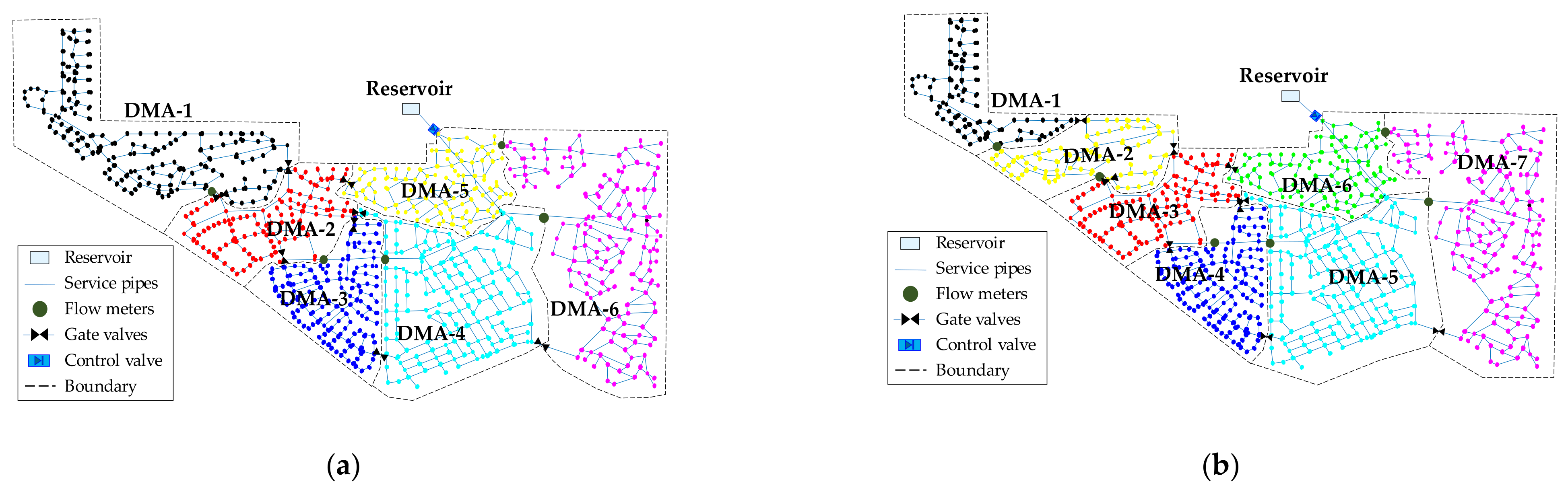
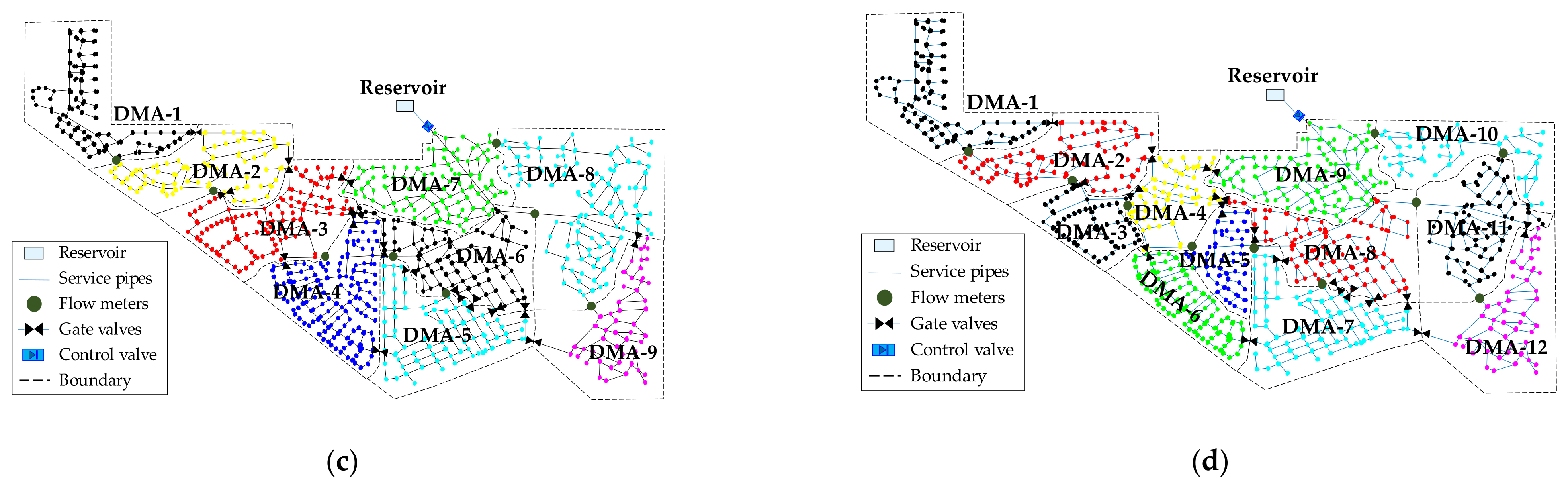
Figure 8d shows the number of DMA solutions versus its modularity index (). As shown in the figure, the index shows a maximum value of approximately 0.89 with 25 DMAs. The index of the layouts with less than 25 DMAs smoothly decreases and falls to 0 when the number of DMAs reaches 1. Here, a desirable number of DMAs in the partitioned layouts is considered for performance analysis based on two aspects: (1) the layouts should have indices larger than 0.3, and (2) the number of DMAs in these layouts should be less than 25. Although layouts with more than 25 DMAs show a sufficiently high index, they are not encouraged to balance the financial investment and the number of DMAs. Thus, the practical layouts with the number of DMA layers between 3 and 25 are evaluated. Figure 9 illustrates four DMA layouts resulting from the coupled model of SOM and CSA. The sectorization results using the GA search for each DMA layout are summarized in Table 4, and the positions of flowmeters and valves in the selected four DMAs are indicated in Figure 9.
Figure 9 shows the change in typical network configurations of the 6, 7, 9, and 12 DMAs. Starting from the six DMA layouts (see Figure 9a) as the initial state, we can progressively see the decomposition. Figure 9b, DMA1 and DMA2 are decomposed from DMA1 in the six DMA layouts, forming a new layout with seven DMAs. The seven DMA design is further decomposed into a nine DMA design by sectorizing DMA5 and DMA7 into two smaller groups (Figure 9c); this DMA design is further decomposed, to finally reach the twelve DMA layout as seen in Figure 9d. In this way, the new DMA layouts that are created by top-down decomposing or bottom-up merging of DMAs always preserve the former layouts (i.e., boundary pipes).
3.3. Comprehensive Evaluation of Alternative DMA Layouts
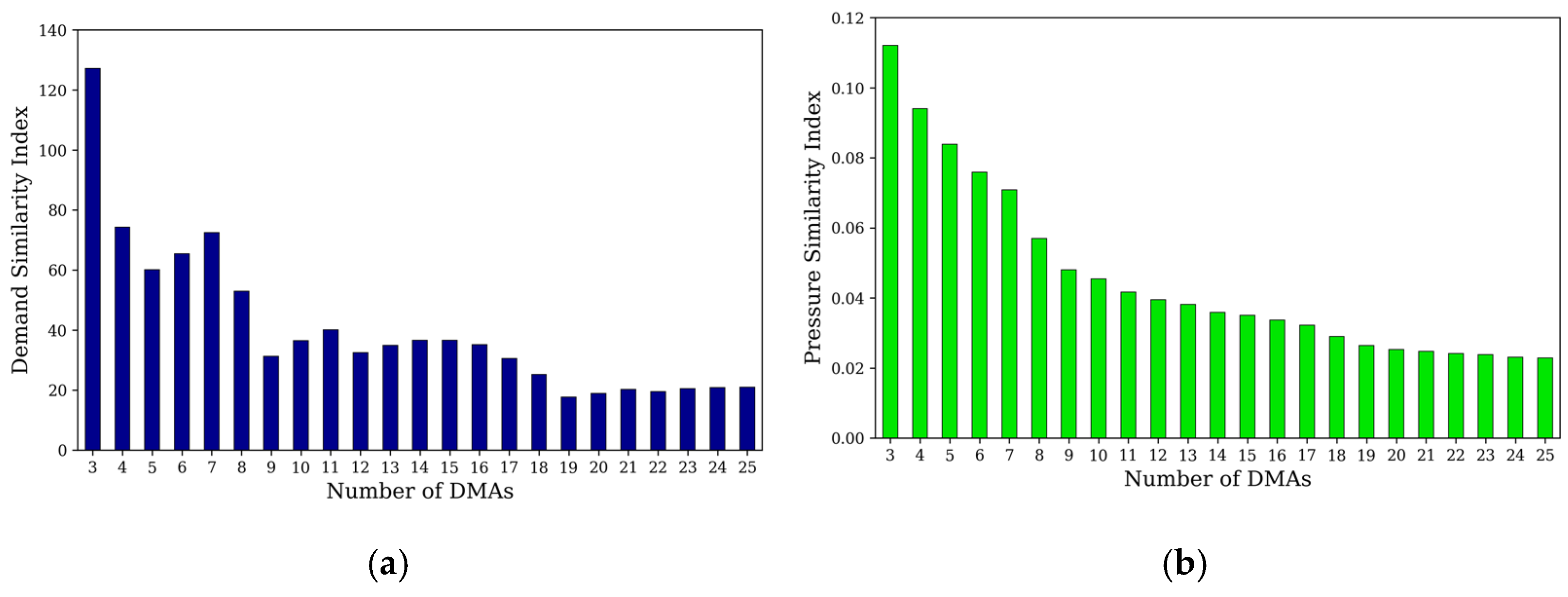
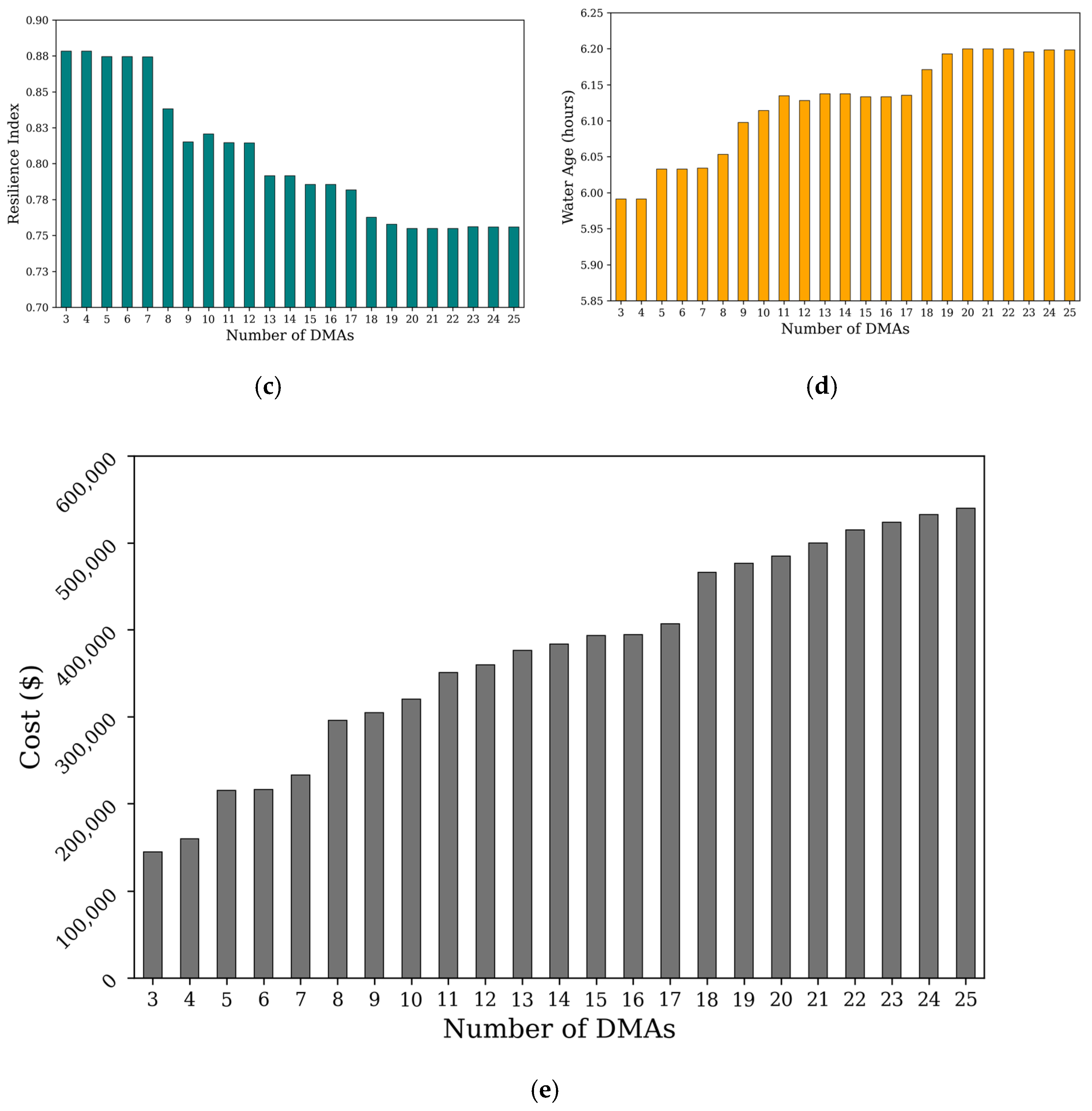
A set of 23 selected DMA layouts (from 3 DMAs to 25 DMAs) were comprehensively evaluated based on their performance. As mentioned in Section 2.5, five criteria were evaluated: (1) demand similarity, (2) pressure similarity, (3) system resilience, (4) WA, and (5) investment cost. The performances of WNP on various criteria are shown in Figure 10.
In general, the more DMAs created, the better is the PSI, as shown in Figure 10b. However, a layout with a greater number of DMAs requires increased investment costs owing to the higher number of devices that need to be installed along the boundary pipes (see Figure 10e). The increase in the number of DMAs also causes a decrease in the RI due to valve closure, as shown in Figure 10c. As expected, the DSI tends to decrease when the number of DMAs increases overall. However, this trend is likely irregular; it fluctuates when the number of DMAs ranges between 3 and 11, as seen in Figure 10a. This indicates that the water demand distribution randomly changes over the application network. As for WA, it tends to increase with the number of DMAs due to valve-controlled isolations. However, there are exceptions; as shown in Figure 10d, the WA decreased slightly either in the case of 12 DMAs or when the number of DMAs increased from 15 to 17. A significant rise in the WA was observed when the number of DMAs ranged from 18 to 25. This can be explained by the fact that the gate valves change the flow direction, thereby increasing or decreasing the flow velocity, resulting in the WA variation.
A decision matrix of 5 × 23 was constructed to evaluate alternative DMA layouts based on the performance criteria. The overall performance scores of the decision matrix after the standardization process are listed in Table 5.
The performance of the individual DMA layouts was ranked by TOPSIS, as summarized in Table 6. The overall results changed irregularly. However, the results show that the 23 layout solutions can be divided into three groups based on their scores, which are relative closeness to the ideal solution. The top scores ranged from 0.655 to 0.679 for the layout solutions containing 5–7 DMAs, followed by a range of scores between 0.612 and 0.645 for designs with 8–10 DMAs. The medium score ranged between 0.509 and 0.576 for the layout containing 11–17 DMAs, and the low scores varied from 0.437 to 0.458 for layouts containing 18–25 DMAs. The highest score calculated was 0.679 for the layout with 7 DMAs. Thus, the evaluation of indicators revealed that the layout containing 7 DMAs was relatively the closest to the ideal solution and was ranked first among the 23 solutions.
The obtained results were compared with those reported by Liu and Han [36], which applied the spectral method for the same Wolf-Cordera Ranch network. The proposed method in this study generates DMA layouts that achieve superior results compared to conventional methods. First, instead of permanent DMAs, the approach proposed here can create dynamic DMAs in which homologous pressures in each DMA are controlled. Second, due to the CSA algorithm’s advantage, with the same number of DMAs, the number of boundary pipes was found to be less than that reported using the spectral method. This plays a vital role in reducing the cost of establishing the DMAs in the network. Third, by proposing an exhaustive analysis of the performance of WNP, the approach proposed here determines the degree of influence of decision-making criteria more plausible. As a result, the best layout was found to be the one with 7 DMAs, compared to the reported 12 DMA layout in the results of Liu and Han [36].
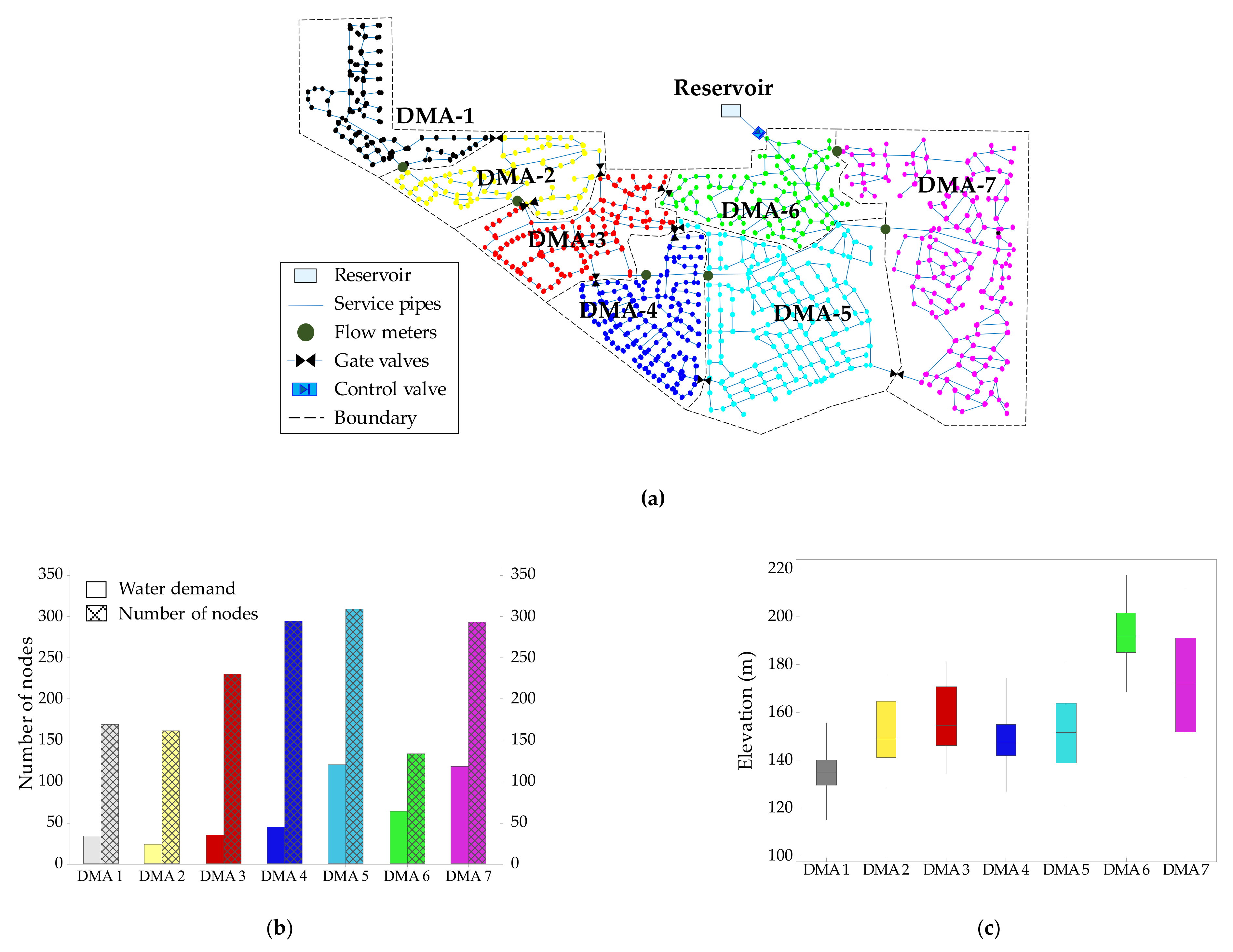
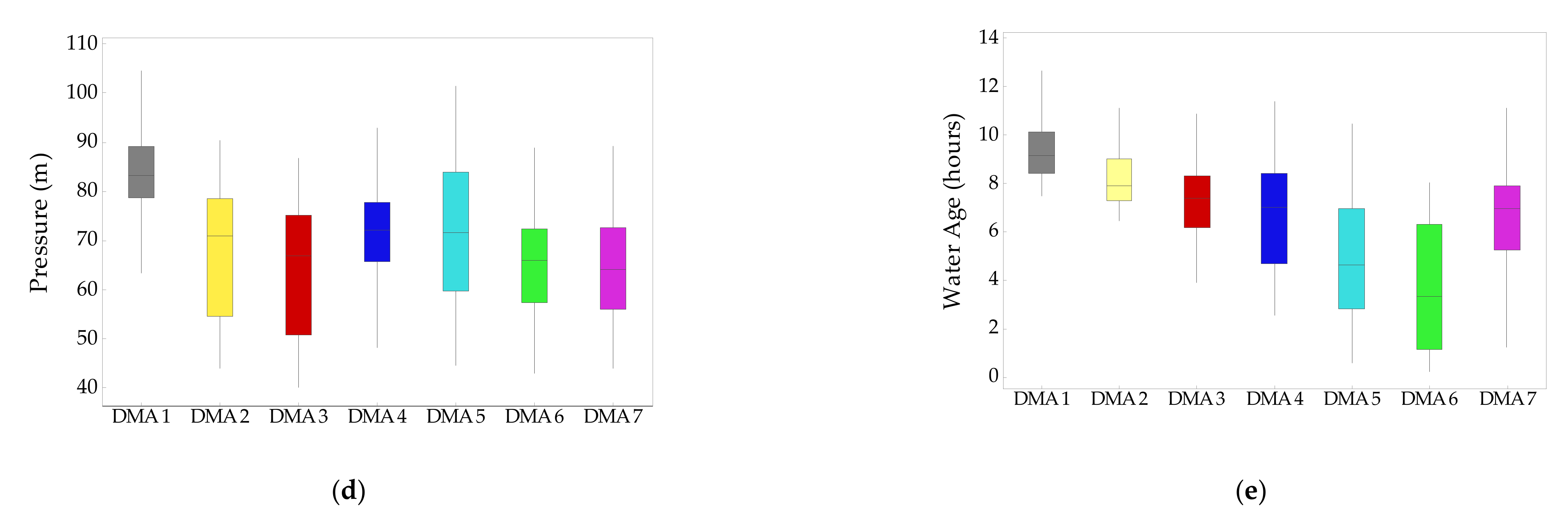
3.4. Evaluation of the Optimal DMA Layout
This section aims to evaluate the operability of the selected optimal layout of 7 DMAs (Figure 11a). The performances of the optimal layout with 7 DMAs are shown in Figure 11b–e. Figure 11b shows the sizes of the DMAs in terms of the water demand and the number of nodes. As shown, the water demand in each DMA varies from 24.1 to 120.7 L/s, with the two largest DMAs being DMA5 and DMA7, whereas the number of nodes changes from 134 for DMA6 to 309 for DMA5. The difference in the water demand between the DMAs can be explained by the fact that the proposed algorithm tends to create DMAs that are homologous in pressure without water demand-based clustering. This is acceptable because, in reality, the water consumption shows random spatial-temporal changes across the network owing to user demand. Figure 11c–e shows the box-whisker plots of various performance indices. Although the Wolf-Cordera Ranch network has an irregular topography with significant variation in the elevation (see Figure 11c), the pressure variations in the DMAs are not significant and the median values are similar to each other as seen in Figure 11d. This is because the proposed algorithm tends to cluster the nodes with similar pressure. The highest-pressure zone was found in DMA1 because it is located in the region with the lowest elevation. On the contrary, DMA6 and DMA7 are located in the higher elevation zones that are close to the reservoir; thus, the pressure is slightly lower than in other zones. The WA tends to increase as the distance from the source to the DMAs increases as seen in Figure 11e. The WA of DMA6 shows wide ranges due to several ending-nodes with very low base demand. In addition, having big and widely spread demand nodes, DMA7 shows a wide range of WA.
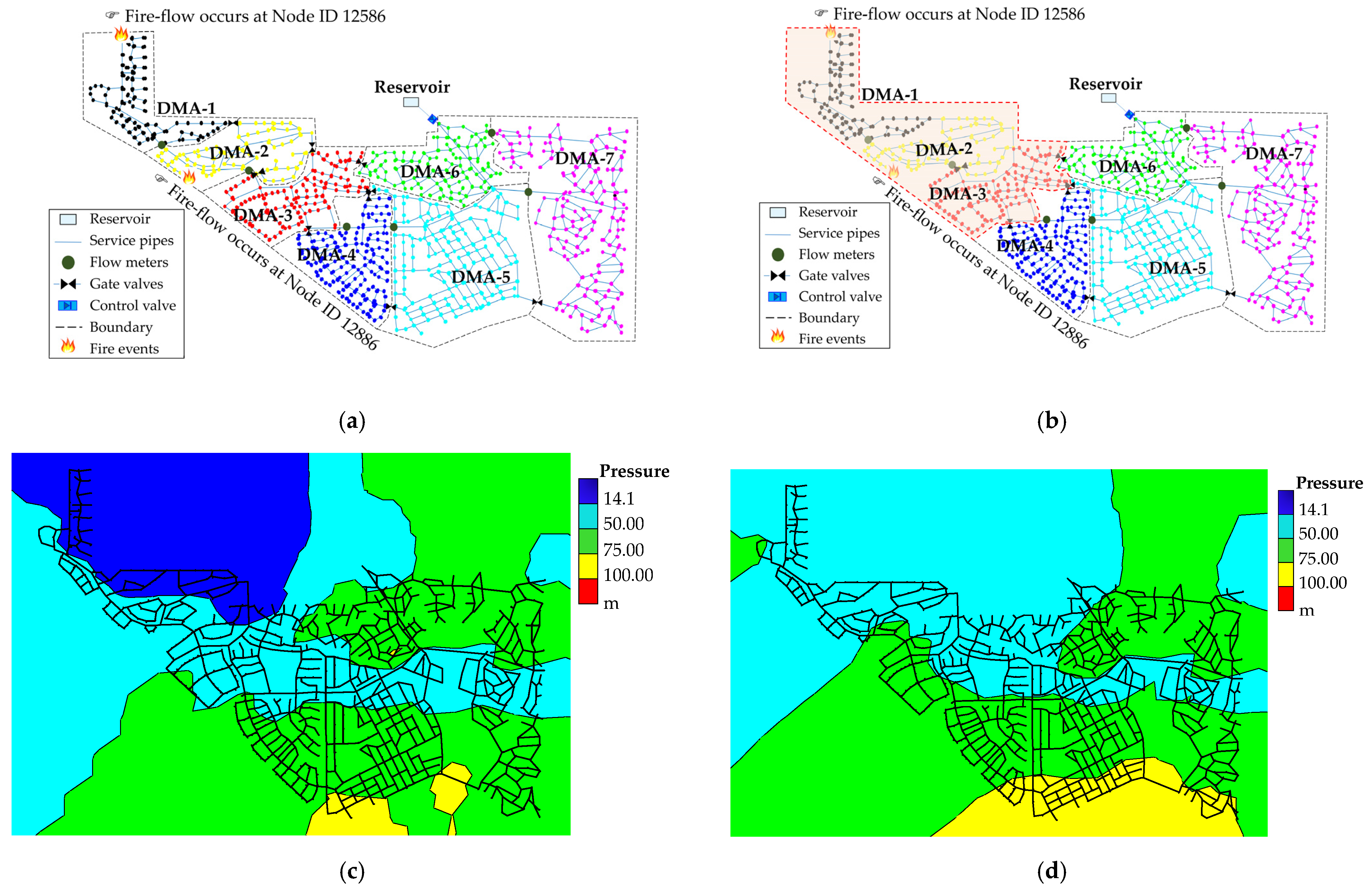
3.5. Dynamic Operation of DMAs
An abnormal operating condition with fire flows was simulated for the selected 7 DMAs layout. Here, the pressure-driven analysis was conducted to simulate the abnormal condition more realistically. Note that a minimum nodal pressure of 14.1 m (20 psi) should be maintained in the entire network during the fire event to supply the network adequately. A central role of the system operation with DMAs is that it provides adequate fire flow and is available for customers at a certain level. This role must be satisfied even when the network is decomposed into DMAs. It was assumed that the fires took place at two separate DMAs at the peak demand hour. A fire flow of 95 L/s (approximately 1500 GPM) was applied equally to the two DMAs. For simplicity, it was assumed that the fire coincided at DMA-1 and DMA-2 because they are critical DMAs with nodes located farthest from the source. Figure 12a shows the original 7 DMAs layout with the locations of the fire occurring nodes.
The analysis revealed that when two fires coincided at two separate DMAs, one at node 12,586 of DMA1 and the other at node 12,886 of DMA2, the network operated at a lower pressure than the required minimum standard (i.e., 14.1 m). Figure 12c shows that the pressures in the upper zones of DMA1, DMA2, and DMA3 were lower than the required pressure of 14.1 m because the head loss in those zones increased owing to the fire flows. To adapt to this situation, the DMAs were merged by opening the gate valves. A dynamic layout can be created by opening some gate valves to merge neighboring DMAs into a larger DMA. In this case, the network was rescaled to a layout containing 5 DMAs by grouping DMA1, DMA2, and DMA3 to a new larger DMA, as depicted in Figure 12b. This was implemented by opening the internal gate valves installed at the boundary pipes 21,244 and 21,775. The nodal pressure in the new layout (i.e., with 5 DMAs) was markedly improved; all nodes within the DMAs guaranteed a higher pressure than the minimum requirement of 14.1 m, as shown in Figure 12d. Furthermore, the pressures in DMA5 and DMA7 were found to increase slightly. This was because opening the gate valves changed the flow directions and reduced head losses.
4. Conclusions
This paper presented an approach for optimizing the design of DMAs in a WDN based on a three-phase strategy. First, the clustering phase generated DMA layouts using a hybrid model of SOM and CSA. Second, in the sectorization phase, the GA was used to locate flowmeters and gate valves for creating isolated DMAs optimally. Finally, five quantitative indicators were introduced to comprehensively evaluate alternative DMA layouts using an MCDA. Following the suggested three phases, the optimal DMA layout for a given WDN was determined both in number and size. The proposed three-phase method was tested on a hypothetical network and an actual complex WDN. The results revealed that the proposed method could auto-create DMAs in terms of homologous pressure by taking full advantage of the SOM model. Moreover, by taking the principle of CSA, the generated configurations of DMAs are dynamic. The dynamic configuration means that new DMA layouts are simplified by aggregation/disaggregation approach while always preserve the set of boundary pipes at each level. Thus, under abnormal conditions such as a fire event, the existing DMA layouts can be transformed dynamically by size-rescaling to make the network more resilient under an emergency.
Constructing the input data for clustering with SOM is crucial. As demonstrated in this study, DMA layouts were generated based on the nodal information without pipe weights. As a future study, it will be interesting to create an input space not only for training SOM but also for any generic WNP algorithms that extend more engineering aspects of WDN, such as existing valves, tanks, pumps, pipe flows, and pipe diameters, to design practical DMAs. The weight factors in MCDA play a critical role in determining the optimal DMA layout. Here, weight factors were determined based on the sound engineering judgment without an objective validation method. Further justification for the determination of the weight factors would be required. Furthermore, an optimization algorithm for identifying the optimal location of gate valves and flowmeters could be extended to consider the influence of tanks, pumps in the O&M of DMAs.
Author Contributions
Conceptualization, X.K.B. and D.K.; methodology, X.K.B. and D.K.; coding and simulation, X.K.B. and M.S.M.; validation, D.K.; formal analysis, X.K.B.; writing—original draft preparation, X.K.B.; writing—review and editing, M.S.M. and D.K.; supervision, D.K.; funding acquisition, D.K. All authors have read and agreed to the published version of the manuscript.
Funding
This work was supported by the National Research Foundation of Korea (NRF) grant funded by the Korean government (MSIT—Ministry of Science and ICT), grant number NRF-2020R1A2C2009517.
Institutional Review Board Statement
Not applicable.
Informed Consent Statement
Not applicable.
Data Availability Statement
The data presented in this study are available on request from the corresponding author.
Conflicts of Interest
The authors declare no conflict of interest.
References
- Farley, M. Leakage Management and Control: A Best Practice Training Manual, No. WHO/SDE/WSH/01.1; World Health Organization: Geneva, Switzerland, 2001. [Google Scholar]
- Morrison, J.; Tooms, S.; Rogers, D. DMA Management Guidance Notes; IWA Publishing: London, UK, 2007. [Google Scholar]
- Di Nardo, A.; Di Natale, M.; Santonastaso, G.F.; Venticinque, S. An Automated Tool for Smart Water Network Partitioning. Water Resour. Manag. 2013, 27, 4493–4508. [Google Scholar] [CrossRef]
- Laucelli, D.B.; Simone, A.; Berardi, L.; Giustolisi, O. Optimal Design of District Metering Areas for the Reduction of Leakages. J. Water Resour. Plan. Manag. 2017, 143, 04017017. [Google Scholar] [CrossRef]
- Rajeswaran, A.; Narasimhan, S.; Narasimhan, S. A graph partitioning algorithm for leak detection in water distribution networks. Comput. Chem. Eng. 2018, 108, 11–23. [Google Scholar] [CrossRef] [Green Version]
- Creaco, E.; Haidar, H. Multiobjective Optimization of Control Valve Installation and DMA Creation for Reducing Leakage in Water Distribution Networks. J. Water Resour. Plan. Manag. 2019, 145, 04019046. [Google Scholar] [CrossRef]
- Brentan, B.; Meirelles, G.; Luvizotto, E.; Izquierdo, J. Hybrid SOM+ k-Means clustering to improve planning, operation and management in water distribution systems. Environ. Model. Softw. 2018, 106, 77–88. [Google Scholar] [CrossRef]
- Ferrari, G.; Savić, D. Economic Performance of DMAs in Water Distribution Systems. Procedia Eng. 2015, 119, 189–195. [Google Scholar] [CrossRef] [Green Version]
- Di Nardo, A.; Di Natale, M.; Musmarra, D.; Santonastaso, G.F.; Tzatchkov, V.; Alcocer-Yamanaka, V.H. Dual-use value of network partitioning for water system management and protection from malicious contamination. J. Hydroinform. 2014, 17, 361–376. [Google Scholar] [CrossRef]
- Di Nardo, A.; Di Natale, M.; Musmarra, D.; Santonastaso, G.; Tuccinardi, F.; Zaccone, G. Software for partitioning and protecting a water supply network. Civ. Eng. Environ. Syst. 2015, 33, 55–69. [Google Scholar] [CrossRef]
- Ciaponi, C.; Creaco, E.; Di Nardo, A.; Di Natale, M.; Giudicianni, C.; Musmarra, D.; Santonastaso, G.F. Reducing Impacts of Contamination in Water Distribution Networks: A Combined Strategy Based on Network Partitioning and Installation of Water Quality Sensors. Water 2019, 11, 1315. [Google Scholar] [CrossRef] [Green Version]
- Gomes, R.; Marques, A.S.A.; Sousa, J. District Metered Areas Design Under Different Decision Makers’ Options: Cost Analysis. Water Resour. Manag. 2013, 27, 4527–4543. [Google Scholar] [CrossRef]
- Di Nardo, A.; Di Natale, M.; Giudicianni, C.; Santonastaso, G.F.; Tzatchkov, V.; Varela, J.M.R. Economic and Energy Criteria for District Meter Areas Design of Water Distribution Networks. Water 2017, 9, 463. [Google Scholar] [CrossRef] [Green Version]
- Herrera, M.; Abraham, E.; Stoianov, I. A Graph-Theoretic Framework for Assessing the Resilience of Sectorised Water Distribution Networks. Water Resour. Manag. 2016, 30, 1685–1699. [Google Scholar] [CrossRef] [Green Version]
- Armand, H.; Stoianov, I.; Graham, N. Impact of network sectorisation on water quality management. J. Hydroinform. 2017, 20, 424–439. [Google Scholar] [CrossRef] [Green Version]
- Boccaletti, S.; Latora, V.; Moreno, Y.; Chavez, M.; Hwang, D. Complex networks: Structure and dynamics. Phys. Rep. 2006, 424, 175–308. [Google Scholar] [CrossRef]
- Saldarriaga, J.; Bohorquez, J.; Celeita, D.; Vega, L.; Paez, D.; Savic, D.; Dandy, G.; Filion, Y.; Grayman, W.; Kapelan, Z. Battle of the Water Networks District Metered Areas. J. Water Resour. Plan. Manag. 2019, 145, 04019002. [Google Scholar] [CrossRef]
- Bui, X.K.; Marlim, M.S.; Kang, D. Water Network Partitioning into District Metered Areas: A State-Of-The-Art Review. Water 2020, 12, 1002. [Google Scholar] [CrossRef] [Green Version]
- Perelman, L.; Ostfeld, A. Topological clustering for water distribution systems analysis. Environ. Model. Softw. 2011, 26, 969–972. [Google Scholar] [CrossRef]
- Lifshitz, R.; Ostfeld, A. Clustering for Analysis of Water Distribution Systems. J. Water Resour. Plan. Manag. 2018, 144, 04018016. [Google Scholar] [CrossRef]
- Scarpa, F.; Lobba, A.; Becciu, G. Elementary DMA Design of Looped Water Distribution Networks with Multiple Sources. J. Water Resour. Plan. Manag. 2016, 142, 04016011. [Google Scholar] [CrossRef] [Green Version]
- Gomes, R.; Marques, A.S.; Sousa, J. Decision support system to divide a large network into suitable District Metered Areas. Water Sci. Technol. 2012, 65, 1667–1675. [Google Scholar] [CrossRef]
- Girvan, M.; Newman, M.E.J. Community structure in social and biological networks. Proc. Natl. Acad. Sci. USA 2002, 99, 7821–7826. [Google Scholar] [CrossRef] [Green Version]
- Clauset, A.; Newman, M.E.J.; Moore, C. Finding community structure in very large networks. Phys. Rev. E 2004, 70, 066111. [Google Scholar] [CrossRef] [Green Version]
- Diao, K.; Zhou, Y.; Rauch, W. Automated Creation of District Metered Area Boundaries in Water Distribution Systems. J. Water Resour. Plan. Manag. 2013, 139, 184–190. [Google Scholar] [CrossRef]
- Campbell, E.; Ayala-Cabrera, D.; Izquierdo, J.; Pérez-García, R.; Tavera, M. Water Supply Network Sectorization Based on Social Networks Community Detection Algorithms. Procedia Eng. 2014, 89, 1208–1215. [Google Scholar] [CrossRef] [Green Version]
- Perelman, L.S.; Allen, M.; Preis, A.; Iqbal, M.; Whittle, A.J. Automated sub-zoning of water distribution systems. Environ. Model. Softw. 2015, 65, 1–14. [Google Scholar] [CrossRef] [Green Version]
- Ciaponi, C.; Murari, E.; Todeschini, S. Modularity-Based Procedure for Partitioning Water Distribution Systems into Independent Districts. Water Resour. Manag. 2016, 30, 2021–2036. [Google Scholar] [CrossRef]
- Giustolisi, O.; Ridolfi, L. New Modularity-Based Approach to Segmentation of Water Distribution Networks. J. Hydraul. Eng. 2014, 140, 04014049. [Google Scholar] [CrossRef]
- Giustolisi, O.; Ridolfi, L. A novel infrastructure modularity index for the segmentation of water distribution networks. Water Resour. Res. 2014, 50, 7648–7661. [Google Scholar] [CrossRef]
- Creaco, E.; Cunha, M.; Franchini, M. Using Heuristic Techniques to Account for Engineering Aspects in Modularity-Based Water Distribution Network Partitioning Algorithm. J. Water Resour. Plan. Manag. 2019, 145, 04019062. [Google Scholar] [CrossRef]
- Simone, A.; Giustolisi, O.; Laucelli, D.B. A proposal of optimal sampling design using a modularity strategy. Water Resour. Res. 2016, 52, 6171–6185. [Google Scholar] [CrossRef] [Green Version]
- Alvisi, S. A New Procedure for Optimal Design of District Metered Areas Based on the Multilevel Balancing and Refinement Algorithm. Water Resour. Manag. 2015, 29, 4397–4409. [Google Scholar] [CrossRef]
- Di Nardo, A.; Di Natale, M.; Giudicianni, C.; Greco, R.; Santonastaso, G.F. Weighted spectral clustering for water distribution network partitioning. Appl. Netw. Sci. 2017, 2, 1–16. [Google Scholar] [CrossRef] [Green Version]
- Di Nardo, A.; Giudicianni, C.; Greco, R.; Herrera, M.; Santonastaso, G.F. Applications of Graph Spectral Techniques to Water Distribution Network Management. Water 2018, 10, 45. [Google Scholar] [CrossRef] [Green Version]
- Liu, J.; Han, R. Spectral Clustering and Multicriteria Decision for Design of District Metered Areas. J. Water Resour. Plan. Manag. 2018, 144, 04018013. [Google Scholar] [CrossRef]
- Izquierdo, J.; Herrera, M.; Montalvo, I.; Pérez-García, R. Agent-based division of water distribution systems into district metered areas. In Proceedings of the 4th International Conference on Software and Data Technologies, Sofia, Bulgaria, 26–29 July 2009; pp. 83–90. [Google Scholar]
- Herrera, M.; Izquierdo, J.; Pérez-García, R.; Montalvo, I. Multi-agent adaptive boosting on semi-supervised water supply clusters. Adv. Eng. Softw. 2012, 50, 131–136. [Google Scholar] [CrossRef]
- Hajebi, S.; Barrett, S.; Clarke, A.; Clarke, S. Multi-agent simulation to support water distribution network partitioning. In Proceedings of the 27th European Simulation and Modelling Conference, Lancaster, UK, 23–25 October 2013; pp. 163–168. [Google Scholar]
- Giudicianni, C.; Herrera, M.; Di Nardo, A.; Adeyeye, K. Automatic Multiscale Approach for Water Networks Partitioning into Dynamic District Metered Areas. Water Resour. Manag. 2020, 34, 835–848. [Google Scholar] [CrossRef] [Green Version]
- Wright, R.; Stoianov, I.; Parpas, P.; Henderson, K.; King, J. Adaptive water distribution networks with dynamically reconfigurable topology. J. Hydroinform. 2014, 16, 1280–1301. [Google Scholar] [CrossRef]
- Liu, J.; Lansey, K.E. Multiphase DMA Design Methodology Based on Graph Theory and Many-Objective Optimization. J. Water Resour. Plan. Manag. 2020, 146, 04020068. [Google Scholar] [CrossRef]
- Pesantez, J.; Berglund, E.Z.; Mahinthakumar, G. Geospatial and Hydraulic Simulation to Design District Metered Areas for Large Water Distribution Networks. J. Water Resour. Plan. Manag. 2020, 146, 06020010. [Google Scholar] [CrossRef]
- Santonastaso, G.F.; Di Nardo, A.; Creaco, E. Dual topology for partitioning of water distribution networks considering actual valve locations. Urban Water J. 2019, 16, 469–479. [Google Scholar] [CrossRef]
- Zhang, K.; Yan, H.; Zeng, H.; Xin, K.; Tao, T. A practical multi-objective optimization sectorization method for water distribution network. Sci. Total. Environ. 2019, 656, 1401–1412. [Google Scholar] [CrossRef]
- Zhang, Q.; Wu, Z.Y.; Zhao, M.; Qi, J.; Huang, Y.; Zhao, H. Automatic Partitioning of Water Distribution Networks Using Multiscale Community Detection and Multiobjective Optimization. J. Water Resour. Plan. Manag. 2017, 143, 04017057. [Google Scholar] [CrossRef]
- Kohonen, T. Self-organized formation of topologically correct feature maps. Biol. Cybern. 1982, 43, 59–69. [Google Scholar] [CrossRef]
- Rana, S.M.M.; Boccelli, D.L.; Marchi, A.; Dandy, G.C. Drinking Water Distribution System Network Clustering Using Self-Organizing Map for Real-Time Demand Estimation. J. Water Resour. Plan. Manag. 2020, 146, 04020090. [Google Scholar] [CrossRef]
- Hwang, C.-L.; Yoon, K. Methods for Multiple Attribute Decision Making. In Optimizing Hospital-Wide Patient Scheduling; Springer: Cham, Switzerland, 2014; pp. 58–191. [Google Scholar]
- Giudicianni, C.; Di Nardo, A.; Di Natale, M.; Greco, R.; Santonastaso, G.F.; Scala, A. Topological Taxonomy of Water Distribution Networks. Water 2018, 10, 444. [Google Scholar] [CrossRef] [Green Version]
- Zhou, T.; Lü, L.; Zhang, Y.-C. Predicting missing links via local information. Eur. Phys. J. B 2009, 71, 623–630. [Google Scholar] [CrossRef] [Green Version]
- Salton, G.; McGill, M.J. Introduction to Modern Information Retrieval; McGraw Hill Book Company: New York, NY, USA, 1983. [Google Scholar]
- Miljkovic, D. Brief review of self-organizing maps. In Proceedings of the 2017 40th International Convention on Information and Communication Technology, Electronics and Microelectronics (MIPRO), Opatija, Croatia, 22–26 May 2017; pp. 1061–1066. [Google Scholar]
- Campbell, E.; Izquierdo, J.; Montalvo, I.; Pérez-García, R. A Novel Water Supply Network Sectorization Methodology Based on a Complete Economic Analysis, Including Uncertainties. Water 2016, 8, 179. [Google Scholar] [CrossRef] [Green Version]
- Newman, M.E.J. Fast algorithm for detecting community structure in networks. Phys. Rev. E 2004, 69, 066133. [Google Scholar] [CrossRef] [Green Version]
- Todini, E. Looped water distribution networks design using a resilience index based heuristic approach. Urban Water 2000, 2, 115–122. [Google Scholar] [CrossRef]
- Ouma, Y.O.; Tateishi, R. Urban Flood Vulnerability and Risk Mapping Using Integrated Multi-Parametric AHP and GIS: Methodological Overview and Case Study Assessment. Water 2014, 6, 1515–1545. [Google Scholar] [CrossRef]
- Chung, E.-S.; Abdulai, P.J.; Park, H.; Kim, Y.; Ahn, S.R.; Kim, S.J. Multi-Criteria Assessment of Spatial Robust Water Resource Vulnerability Using the TOPSIS Method Coupled with Objective and Subjective Weights in the Han River Basin. Sustain. J. Rec. 2016, 9, 29. [Google Scholar] [CrossRef] [Green Version]
- Martínez-Solano, F.J.; Iglesias-Rey, P.L.; Meliá, D.M.; Ribelles-Aguilar, J.V. Combining Skeletonization, Setpoint Curves, and Heuristic Algorithms to Define District Metering Areas in the Battle of Water Networks District Metering Areas. J. Water Resour. Plan. Manag. 2018, 144, 04018023. [Google Scholar] [CrossRef]
- Salomons, E.; Skulovich, O.; Ostfeld, A. Battle of Water Networks DMAs: Multistage Design Approach. J. Water Resour. Plan. Manag. 2017, 143, 04017059. [Google Scholar] [CrossRef]
- Lippai, I. Water System Design by Optimization: Colorado Springs Utilities Case Studies. In Pipelines 2005; American Society of Civil Engineers (ASCE): Reston, VA, USA, 2005; pp. 1058–1070. [Google Scholar]
Figure 1.
Flow chart of the proposed approach.

Figure 2.
Illustration of self-organizing map (SOM) model: (a) two-layer SOM for community detection; (b) schematic to illustrate the performance of SOM to determine district metered areas (DMAs) in water distribution network (WDN).
Figure 2.
Illustration of self-organizing map (SOM) model: (a) two-layer SOM for community detection; (b) schematic to illustrate the performance of SOM to determine district metered areas (DMAs) in water distribution network (WDN).

Figure 3.
Flowchart of the clustering approach.

Figure 4.
Sample network illustration: (a) WDN layout and (b) variation in pressure and elevation at nodes.
Figure 4.
Sample network illustration: (a) WDN layout and (b) variation in pressure and elevation at nodes.

Figure 5.
Construction of attribute matrices for the sample network. (a) Adjacency matrix (A) obtained from Equation (1); (b) TS matrix obtained from Equation (3); (c) HS matrix obtained from Equation (4); (d) Input matrix (X) for training the SOM obtained from Equation (7).
Figure 5.
Construction of attribute matrices for the sample network. (a) Adjacency matrix (A) obtained from Equation (1); (b) TS matrix obtained from Equation (3); (c) HS matrix obtained from Equation (4); (d) Input matrix (X) for training the SOM obtained from Equation (7).


Figure 6.
Results of training a SOM model for a sample network: (a) U-Matrix map of 3 × 3 neurons; (b) nine initial clusters obtained after training the SOM.
Figure 6.
Results of training a SOM model for a sample network: (a) U-Matrix map of 3 × 3 neurons; (b) nine initial clusters obtained after training the SOM.

Figure 7.
Post-partition results of the CSA: (a–h) multiscale DMA layouts (from 9 to 2 DMAs); (i) variation in modularity index with the number of DMAs.
Figure 7.
Post-partition results of the CSA: (a–h) multiscale DMA layouts (from 9 to 2 DMAs); (i) variation in modularity index with the number of DMAs.

Figure 8.
Formation of DMAs in the Wolf-Cordera Ranch water distribution network through the proposed method: (a) the original WDN, (b) the U-matrix with nodal hits labeled in each cluster, (c) SOM initial clusters abstracted to the WDN, and (d) modularity indexes for the corresponding number of DMAs following the application of CSA.

Figure 9.
Sample of DMA layouts generated: (a) 6 DMAs; (b) 7 DMAs; (c) 9 DMAs; (d) 12 DMAs.


Figure 10.
Performance of different DMA layouts on various criteria: (a) DSI; (b) PSI; (c) RI; (d) WA; (e) investment costs (Cost).
Figure 10.
Performance of different DMA layouts on various criteria: (a) DSI; (b) PSI; (c) RI; (d) WA; (e) investment costs (Cost).


Figure 11.
Performance of optimal layout with 7 DMAs operating under the normal condition: (a) DMA layout; (b) bar chart representing the size of each DMA; (c–e) show the variations in elevation, pressure, and WA, respectively, in each DMA.
Figure 11.
Performance of optimal layout with 7 DMAs operating under the normal condition: (a) DMA layout; (b) bar chart representing the size of each DMA; (c–e) show the variations in elevation, pressure, and WA, respectively, in each DMA.


Figure 12.
Simulation of fire-flow scenario: (a) original 7 DMAs layout with fire events; (b) network adaptation by merging DMAs 1, 2, and 3 into one larger DMA; (c) contour plot of pressure for original 7 DMAs layout under fire events; (d) contour plot of pressure after DMAs merging by opening the gate valves under fire events.


Table 1.
Results for sample network clustering and comparison of performance.
| No. of Clusters | Cluster Record | Variance Record | Average Variance | Q Index |
|---|---|---|---|---|
| 9 | C1 = {1,2,3}; C2 = {4,5,6,7}; C3 = {8}; C4 = {9,10,11,12}; C5 = {13}; C6 = {14,15,16}; C7 = {17}; C8 = {18,19,20}; C9 = {21,22,23}; | Var(C1) = 0.0056; Var(C2) = 0.0873; Var(C3) = 0; Var(C4) = 0.0135; Var(C5) = 0; Var(C6) = 0.0423; Var(C7) = 0; Var(C8) = 0.0261; Var(C9) = 0.0838; | 0.0287 | 0.4511 |
| 8 | C1 = {1,2,3}; C2 = {4,5,6,7}; C3 = {8, 13}; C4 = {9,10,11,12}; C5 = {14,15,16}; C6 = {17}; C7 = {18,19,20}; C8 = {21,22,23}; | Var(C1) = 0.0056; Var(C2) = 0.0873; Var(C3) = 1.0898; Var(C4) = 0.0135; Var(C5) = 0.0423; Var(C6) = 0; Var(C7) = 0.0261; Var(C8) = 0.0838 | 0.1686 | 0.4767 |
| 7 | C1 = {1,2,3}; C2 = {4,5,6,7}; C3 = {8,9,10,11,12,13}; C4 = {14,15,16}; C5 = {18,19,20}; C6 = {17}; C7 = {21,22,23}; | Var(C1) = 0.0056; Var(C2) = 0.0873; Var(C3) = 0.7191; Var(C4) = 0.0423; Var(C5) = 0.0261; Var(C6) = 0; Var(C7) = 0.0838 | 0.1377 | 0.5211 |
| 6 | C1 = {1,2,3}; C2 = {4,5,6,7}; C3 = {8,9,10,11,12,13}; C4 = {14,15,16}; C5 = {18,19,20}; C6 = {17,21,22,23}; | Var(C1) = 0.0056; Var(C2) = 0.0873; Var(C3) = 0.7191; Var(C4) = 0.0423; Var(C5) = 0.0261; Var(C6) = 0.0642; | 0.1574 | 0.5422 |
| 5 | C1 = {1,2,3}; C2 = {4,5,6,7}; C3 = {8,9,10,11,12,13}; C4 = {14,15,16}; C5 = {17,18,19,20,21,22,23}; | Var(C1) = 0.0056; Var(C2) = 0.0873; Var(C3) = 0.7191; Var(C4) = 0.0423; Var(C5) = 0.0506; | 0.1810 | 0.5433 |
| 4 | C1 = {1,2,3,14,15,16}; C2 = {4,5,6,7}; C3 = {8,9,10,11,12,13}; C4 = {17,18,19,20,21,22,23}; | Var(C1) = 7.1598; Var(C2) = 0.0873; Var(C3) = 0.7191; Var(C4) = 0.0506; | 2.0042 | 0.5422 |
| 3 | C1 = {1,2,3,14,15,16}; C2 = {4,5,6,7,8,9,10,11,12,13}; C3 = {17,18,19,20,21,22,23}; | Var(C1) = 7.1598; Var(C2) = 5.3974; Var(C3) = 0.0506; | 4.2026 | 0.4700 |
| 2 | C1 = {1,2,3,4,5,6,7,8,9,10,11,12, 13,14,15,16}; C2 = {17,18,19,20,21,22,23}; | Var(C1) = 6.1588; Var(C2) = 0.0506; | 3.1047 | 0.3389 |
Table 2.
Weight factors for MCDA model.
| Indicator | DSI | PSI | RI | WA | Cost |
|---|---|---|---|---|---|
| Weight | 0.2 | 0.3 | 0.2 | 0.1 | 0.2 |
Table 3.
Main characteristics of the Wolf-Cordera Ranch water distribution network.
| Physical Characteristics | Value | Main Hydraulic Features | Value |
|---|---|---|---|
| No. of nodes | 1592 | Minimum pressure (m): | 41.2 |
| No. of pipes | 1795 | Mean of pressure (m): | 70.8 |
| No. of valves (PRVs) | 2 | Maximum pressure (m): | 107.7 |
| No. of reservoirs | 1 | Mean surplus pressure (m): | 29.1 |
| No. of pumping stations | 1 | Average WA (hour): | 6.0 |
| Main pipe diameters (mm) | 200–600 | Resilience index (RI) | 0.877 |
Note that the proposed methods were developed in the MATLAB environment version R2020a, supported with the Epanet-Matlab toolkit for hydraulic simulation. The program was run using an Intel Core i9-10920X @ 3.5 GHz (24 CPUs) and 128 GB RAM on a Windows 10 environment.
Table 4.
Characteristic of boundary pipes obtained by GA for different DMA layouts.
| No. of DMAs | |||||||||||||||||||||||
|---|---|---|---|---|---|---|---|---|---|---|---|---|---|---|---|---|---|---|---|---|---|---|---|
| 3 | 4 | 5 | 6 | 7 | 8 | 9 | 10 | 11 | 12 | 13 | 14 | 15 | 16 | 17 | 18 | 19 | 20 | 21 | 22 | 23 | 24 | 25 | |
| Nbp | 9 | 10 | 12 | 13 | 15 | 23 | 25 | 27 | 30 | 33 | 35 | 36 | 38 | 39 | 44 | 48 | 51 | 53 | 54 | 55 | 56 | 58 | 59 |
| Nfm | 3 | 4 | 5 | 5 | 6 | 7 | 8 | 9 | 10 | 11 | 12 | 13 | 14 | 14 | 15 | 16 | 17 | 18 | 19 | 20 | 21 | 22 | 23 |
| Ngv | 6 | 6 | 7 | 8 | 9 | 16 | 17 | 18 | 20 | 22 | 23 | 23 | 24 | 25 | 29 | 32 | 34 | 35 | 35 | 35 | 35 | 36 | 36 |
Note: Nbp, Nfm, and Ngv are the number of boundary pipes, flowmeters, and gate valves, respectively.
Table 5.
Standardization of performance indices for 23 DMA layouts.
| No. of DMAs | Criteria | ||||
|---|---|---|---|---|---|
| DSI | PSI | RI | WA | Cost | |
| 3-DMAs | 0.00 | 0.00 | 1.00 | 1.00 | 1.00 |
| 4-DMAs | 0.48 | 0.20 | 1.00 | 1.00 | 0.96 |
| 5-DMAs | 0.61 | 0.32 | 0.97 | 0.80 | 0.82 |
| 6-DMAs | 0.56 | 0.41 | 0.97 | 0.80 | 0.82 |
| 7-DMAs | 0.50 | 0.46 | 0.97 | 0.79 | 0.78 |
| 8-DMAs | 0.68 | 0.62 | 0.67 | 0.70 | 0.62 |
| 9-DMAs | 0.88 | 0.72 | 0.49 | 0.49 | 0.59 |
| 10-DMAs | 0.83 | 0.75 | 0.53 | 0.41 | 0.56 |
| 11-DMAs | 0.79 | 0.79 | 0.48 | 0.31 | 0.48 |
| 12-DMAs | 0.87 | 0.81 | 0.48 | 0.34 | 0.46 |
| 13-DMAs | 0.84 | 0.83 | 0.30 | 0.30 | 0.41 |
| 14-DMAs | 0.83 | 0.85 | 0.30 | 0.30 | 0.40 |
| 15-DMAs | 0.83 | 0.86 | 0.25 | 0.32 | 0.37 |
| 16-DMAs | 0.84 | 0.88 | 0.25 | 0.32 | 0.37 |
| 17-DMAs | 0.88 | 0.90 | 0.22 | 0.31 | 0.34 |
| 18-DMAs | 0.93 | 0.93 | 0.06 | 0.14 | 0.19 |
| 19-DMAs | 1.00 | 0.96 | 0.02 | 0.03 | 0.16 |
| 20-DMAs | 0.99 | 0.97 | 0.00 | 0.00 | 0.14 |
| 21-DMAs | 0.98 | 0.98 | 0.00 | 0.00 | 0.10 |
| 22-DMAs | 0.98 | 0.99 | 0.00 | 0.00 | 0.06 |
| 23-DMAs | 0.97 | 0.99 | 0.01 | 0.02 | 0.04 |
| 24-DMAs | 0.97 | 1.00 | 0.01 | 0.01 | 0.02 |
| 25-DMAs | 0.97 | 1.00 | 0.01 | 0.01 | 0.00 |
Table 6.
Ranking of DMA layouts by the TOPSIS method.
| No. of DMAs | Criterion | E+ | E− | C | Rank | ||||
|---|---|---|---|---|---|---|---|---|---|
| DSI | PSI | RI | WA | Cost | |||||
| 3 DMAs | 0.0000 | 0.0000 | 0.0777 | 0.0425 | 0.0806 | 0.0933 | 0.1198 | 0.5621 | 10 |
| 4 DMAs | 0.0244 | 0.0159 | 0.0777 | 0.0425 | 0.0775 | 0.0679 | 0.1213 | 0.6412 | 5 |
| 5 DMAs | 0.0310 | 0.0248 | 0.0754 | 0.0341 | 0.0662 | 0.0595 | 0.1131 | 0.6552 | 3 |
| 6 DMAs | 0.0285 | 0.0319 | 0.0754 | 0.0341 | 0.0659 | 0.0543 | 0.1141 | 0.6776 | 2 |
| 7 DMAs | 0.0253 | 0.0363 | 0.0753 | 0.0338 | 0.0626 | 0.0531 | 0.1126 | 0.6794 | 1 |
| 8 DMAs | 0.0343 | 0.0485 | 0.0524 | 0.0299 | 0.0497 | 0.0540 | 0.0982 | 0.6451 | 4 |
| 9 DMAs | 0.0443 | 0.0563 | 0.0380 | 0.0208 | 0.0479 | 0.0604 | 0.0965 | 0.6151 | 6 |
| 10 DMAs | 0.0419 | 0.0586 | 0.0415 | 0.0175 | 0.0448 | 0.0608 | 0.0960 | 0.6123 | 7 |
| 11 DMAs | 0.0402 | 0.0619 | 0.0377 | 0.0133 | 0.0385 | 0.0679 | 0.0923 | 0.5761 | 9 |
| 12 DMAs | 0.0438 | 0.0638 | 0.0375 | 0.0146 | 0.0367 | 0.0677 | 0.0946 | 0.5831 | 8 |
| 13 DMAs | 0.0426 | 0.0650 | 0.0232 | 0.0127 | 0.0334 | 0.0796 | 0.0886 | 0.5267 | 11 |
| 14 DMAs | 0.0419 | 0.0670 | 0.0232 | 0.0127 | 0.0319 | 0.0803 | 0.0892 | 0.5261 | 12 |
| 15 DMAs | 0.0418 | 0.0677 | 0.0194 | 0.0135 | 0.0299 | 0.0837 | 0.0883 | 0.5132 | 14 |
| 16 DMAs | 0.0425 | 0.0689 | 0.0194 | 0.0135 | 0.0296 | 0.0837 | 0.0894 | 0.5166 | 13 |
| 17 DMAs | 0.0447 | 0.0702 | 0.0169 | 0.0131 | 0.0271 | 0.0868 | 0.0901 | 0.5093 | 15 |
| 18 DMAs | 0.0471 | 0.0731 | 0.0049 | 0.0059 | 0.0150 | 0.1048 | 0.0886 | 0.4579 | 16 |
| 19 DMAs | 0.0506 | 0.0753 | 0.0019 | 0.0014 | 0.0130 | 0.1097 | 0.0916 | 0.4552 | 17 |
| 20 DMAs | 0.0500 | 0.0763 | 0.0000 | 0.0000 | 0.0112 | 0.1126 | 0.0919 | 0.4495 | 18 |
| 21 DMAs | 0.0494 | 0.0768 | 0.0000 | 0.0000 | 0.0081 | 0.1145 | 0.0916 | 0.4446 | 19 |
| 22 DMAs | 0.0497 | 0.0773 | 0.0000 | 0.0000 | 0.0051 | 0.1164 | 0.0921 | 0.4415 | 20 |
| 23 DMAs | 0.0493 | 0.0775 | 0.0008 | 0.0008 | 0.0033 | 0.1167 | 0.0920 | 0.4406 | 21 |
| 24 DMAs | 0.0491 | 0.0782 | 0.0007 | 0.0003 | 0.0015 | 0.1182 | 0.0924 | 0.4388 | 22 |
| 25 DMAs | 0.0491 | 0.0784 | 0.0007 | 0.0003 | 0.0000 | 0.1192 | 0.0925 | 0.4369 | 23 |
| Best ideal | 0.0506 | 0.0784 | 0.0777 | 0.0425 | 0.0806 | ||||
| Worst ideal | 0.0000 | 0.0000 | 0.0000 | 0.0000 | 0.0000 | ||||
Note: and denote the distance from the evaluated object to the best and worst ideal solutions (obtained by Equation (34)), respectively, while is the relative closeness of the evaluation object to the ideal solution (obtained by Equation (35)).
Publisher’s Note: MDPI stays neutral with regard to jurisdictional claims in published maps and institutional affiliations. |
© 2021 by the authors. Licensee MDPI, Basel, Switzerland. This article is an open access article distributed under the terms and conditions of the Creative Commons Attribution (CC BY) license (http://creativecommons.org/licenses/by/4.0/).
Share and Cite
MDPI and ACS Style
Bui, X.K.; Marlim, M.S.; Kang, D. Optimal Design of District Metered Areas in a Water Distribution Network Using Coupled Self-Organizing Map and Community Structure Algorithm. Water 2021, 13, 836. https://doi.org/10.3390/w13060836
AMA Style
Bui XK, Marlim MS, Kang D. Optimal Design of District Metered Areas in a Water Distribution Network Using Coupled Self-Organizing Map and Community Structure Algorithm. Water. 2021; 13(6):836. https://doi.org/10.3390/w13060836
Chicago/Turabian StyleBui, Xuan Khoa, Malvin S. Marlim, and Doosun Kang. 2021. "Optimal Design of District Metered Areas in a Water Distribution Network Using Coupled Self-Organizing Map and Community Structure Algorithm" Water 13, no. 6: 836. https://doi.org/10.3390/w13060836
Note that from the first issue of 2016, this journal uses article numbers instead of page numbers. See further details here.