
A Site-Scale Tool for Performance-Based Design of Stormwater Best Management Practices


1
Civil and Environmental Engineering Department, South Dakota School of Mines and Technology, Rapid City, SD 57701, USA
2
City and County of Denver, Office of Green Infrastructure, Department of Transportation and Infrastructure, Denver, CO 80223, USA
3
Civil and Environmental Engineering Department, Colorado School of Mines, Golden, CO 80401, USA
*
Authors to whom correspondence should be addressed.
Water 2021, 13(6), 844; https://doi.org/10.3390/w13060844
Submission received: 31 January 2021
/
Revised: 10 March 2021
/
Accepted: 12 March 2021
/
Published: 19 March 2021
(This article belongs to the Special Issue Cross-Sector Green Infrastructure for Improving Urban Storm Water Quality)
Abstract
:The objective of this research is to develop a module for the design of best management practices based on percent pollutant removal. The module is a part of the site-scale integrated decision support tool (i-DSTss) that was developed for stormwater management. The current i-DSTss tool allows for the design of best management practices based on flow reduction. The new water quality module extends the capability of the i-DSTss tool by adding new procedures for the design of best management practices based on treatment performance. The water quality module can be used to assess the treatment of colloid/total suspended solid and dissolved pollutants. We classify best management practices into storage-based (e.g., pond) and infiltration-based (e.g., bioretention and permeable pavement) practices for design purposes. Several of the more complex stormwater tools require expertise to build and operate. The i-DSTss and its component modules including the newly added water quality module are built on an accessible platform (Microsoft Excel VBA) and can be operated with a minimum skillset. Predictions from the water quality module were compared with observed data, and the goodness-of-fit was evaluated. For percent total suspended solid removal, both R2 and Nash–Sutcliffe efficiency values were greater than 0.7 and 0.6 for infiltration-based and storage-based best management practices, respectively, demonstrating a good fit for both types of best management practices. For percent total phosphorous and Escherichia. coli removal, R2 and Nash–Sutcliffe efficiency values demonstrated an acceptable fit. To enhance usability of the tool by a broad range of users, the tool is designed to be flexible allowing user interaction through a graphical user interface.
1. Introduction
Increased building, roadway, and parking lot densities associated with urbanization result in an expansion of impervious cover in urban watersheds. Impervious surfaces do not allow for the natural infiltration of stormwater and lead to increased runoff volumes, peak flow rates, and decreased water quality in the watershed’s receiving water body [1,2,3]. Impervious surfaces also accumulate pollutants, such as trash, gasoline, and fertilizers, that can adversely affect the water quality in the receiving water body as they are washed off during storm events [4]. These pollutants disrupt the natural environment by impacting certain aquatic species; promoting eutrophication, which leads to oxygen depletion and clogging of waterways; and increasing the potential for human health hazards [5,6,7]. Best management practices (BMPs) are evolving stormwater management approaches using natural processes to mitigate stormwater runoff and water quality. BMPs include structural, vegetative, or managerial practices used to treat, prevent, or reduce water pollution. In this study, we group BMPs in two categories: infiltration-based and storage-based BMPs. The infiltration-based BMPs alter runoff from drainage areas through infiltration while storage-based BMPs alter runoff mainly though storage. BMPs are implemented to achieve an integrated stormwater management using multiple BMP options [8]. Management of stormwater runoff quality and quantity using BMPs is a multi-benefit solution that can address both stormwater quality and quantity concerns [9,10].
BMP design for water quality improvement is often based on assumed performance or non-site-specific empirical estimation rather than premised on a fundamental understanding of pollutant removal mechanisms for the specific BMP at a specific site [11]. Thus, BMP design tools capable of more detailed analysis of water quality improvement are needed. More research is needed to properly characterize the interactions between hydrologic impacts of BMPs, processes for contaminant removal, and water quality performance.
An initial version of the tool (i-DSTss: site-scale integrated decision support tool) was developed for the design of BMPs based on flow reduction only [12]. A new water quality module was added to i-DSTss during this study. Thus, the current version of the i-DSTss allows the design of BMPs based on flow reduction and/or percent pollutant removal. The i-DSTss is a stormwater management model developed by the research team for the design of BMPs based on flow reduction [12,13]. The water quality module within i-DSTss includes a physically based mass balance approach for the design of infiltration- and storage-based BMPs according to percent pollutant removal.
Pollutant removal processes vary based on both type of BMPs and type of pollutants. Removal processes may include sedimentation, filtration, infiltration, and adsorption. Sedimentation involves the gravitational settling of suspended particles from runoff in ponds and infiltration-based BMPs such as bioretention cells. This is also a major mechanism for some pollutants that sorb to particulate matter and settle (e.g., phosphorus) [14]. Filtration removes particulates as they pass through a porous medium such as sand, vegetation, soil mixes, and gravel [15]. Pollutants can also be removed in infiltration-based BMPs as stormwater infiltrates into the aquifer [16]. Pollutants can also be removed in BMPs through sorption on to soil mixes and organic filters [17].
The physical, chemical, and biological process occurring in BMPs are complex; thus, detailed procedures are required for calculating BMP efficiency and effectiveness. Detailed models can be calibrated to capture observational data more accurately than over-simplified models. The International Stormwater BMP Database is a publicly accessible repository for BMP performance, design, and cost information. The project website features a database of over 700 BMP studies, performance analysis results, tools for use in BMP performance studies, monitoring guidance, and other study-related publications [18]. The database is the result of an effort by the Environmental Protection Agency (EPA) to collect stormwater quality data in the United States. It includes the concentration of different pollutant types, such as Total Suspended Solid (TSS), phosphorous, and other types of pollutants, collected from different EPA rainfall zones. The database characterizes BMP performance based on event mean concentration (EMC). The EMC is a key analytical parameter defined as the total pollution load (M) divided by the total runoff volume (L3) [19]. Although some groups believe that a better method for measuring performance is the amount of flow treated and effluent quality [20], an outlet EMC value is probably the simplest single measure of BMP performance. While an outlet EMC may be an appropriate method for determining the reduction in pollutant concentrations for an individual event, an EMC may not give an indication of the long-term performance of the BMP or the performance for runoff events of varying intensity and volume [21]. The outlet EMC model could be a good option when site-specific EMC data are available and when physically based models could not sufficiently describe the pollutant removal phenomena. The use of literature data based on land use may limit the accuracy of this EMC approach due to the variabilities in climatologic and physiographic characteristics of individual watersheds.
Strecker et al. (2001) discussed the challenges of using monitoring data to develop consistent estimates of BMP effectiveness and pollutant removal [20]. Thus, modeling these processes at a fundamental level requires estimation of pollutant removal based on physical design parameters, hydraulic variables, and intrinsic chemical properties and reaction rates. Several models have been developed to estimate the pollutant removal capacities of BMPs. The Minnesota Pollution Control Agency (MPCA) Estimator worksheet [22] presents a calculator approach to computing the pollutant load reduction for total phosphorus (TP) and TSS with a simple method. The estimator applies only to specific structural stormwater BMPs and is a simplistic tool that provides estimates of loading and load reductions. Therefore, it is not an appropriate tool for modeling a stormwater system or selecting BMPs. The estimator computes pollutant reduction using BMP performance data from the International BMP Database [18].
In some of the previous tools, the size of BMPs was determined as a function of drainage area, imperviousness, flow rate, pollutant loads, depth of BMP, and infiltration rate. Examples include the Minimal Impact Design Standards (MIDs) calculator [23] and the California Phase II Low Impact Development (LID) Sizing Tool [24]. These tools developed a graph that relates percent flow captured or percent pollutant reduction to a sizing factor (a dimensionless area, which is the ratio of the area of the BMP to the drainage area). The limitation of these approaches is that the performance curves are just applicable to the specific sites. A more robust approach was developed and implemented in the current water quality module, describing the relationship between percent pollutant removal.
Pollutant removal is often estimated using first-order decay kinetics [25,26]. The commonly applied Storm Water Management Model (SWMM) uses a conceptual continuous-flow, stirred-tank reactor (CFSTR) model to model water quality treatment in impoundments [27]. Conceptually, the CFSTR represents all treatment or removal processes that act to reduce EMCs of constituents as they pass through the BMP. The use of empirical approaches and constant concentration (EMC) for water quality prediction include assumptions that could potentially limit the accuracy of such models [28]. This method does not account for the loss of water by infiltration and evapotranspiration, which acts to reduce loads especially for BMP facilities. However, SWMM simulation also accounts for storage changes during inflows to and outflows from the facility. The main removal mechanism available with SWMM is first-order decay.
Similar to the CFSTR approach in SWMM [27], System for Urban Stormwater Treatment and Analysis IntegratioN (SUSTAIN) [29] implements first-order reaction decay for pollutant removal by BMPs. These models are relatively complex, require extensive data processing, and modeling expertise to set up and operate. Other simplified tools presented earlier are based on simplified empirical approaches such as the Minnesota Pollution Control Agency (MPCA) Estimator tool [22]. The prediction accuracy of these simplified tools is low relative to that of the more complex tools, and they are usually applicable to the specific location where they were initially developed. The water quality module within i-DSTss is user-friendly and includes rigorous approaches used in the more complex tools (e.g., SUSTAIN). The water quality module within i-DSTss can be used to calculate BMP removal efficiency for multiple types of BMPs based on user-defined data such as BMP geometry and BMP characteristics (e.g., soil type, depth, and surface area).
A significant merit of the i-DSTss water quality module is that complex approaches were translated into easy to use, computationally less intensive, yet rigorous, physically based modules. In the development of the water quality module, attempts were made to make a balance between model accuracy, model parsimony, and model transparency, which are the fundamental principles of model development [30]. The limitation of the water quality module is that it considers more parameters, e.g., soil type and decay rate, than simple models. The current water quality module uses generic default values for some parameters (e.g., decay rate). Other parameters are populated according to soil type based on literature values. Thus, the tool requires site-specific parameter values or the determination of more realistic values via calibration to yield better results. The limitation of the current tool is that it requires the influent concentration to be provided by the user. Future modifications should connect the tool to the National Stormwater Quality Database (NSQD) [31]. The advantage of the water quality module is that it is developed on the commonly used Excel-VBA platform, which requires minimum skillset, allowing a broader use.
The objective of this study is to develop and demonstrate a relatively detailed but easy-to-use sizing tool that can be used to design different types of BMPs based on water quality in urban watersheds. The water quality module is capable of analyzing scenarios of tradeoffs between BMP size and percent pollutant reduction. The result of the water quality module was verified with observed data for a permeable pavement and a wet detention pond in Madison, Wisconsin.
2. Methodology
2.1. Water Quality Module
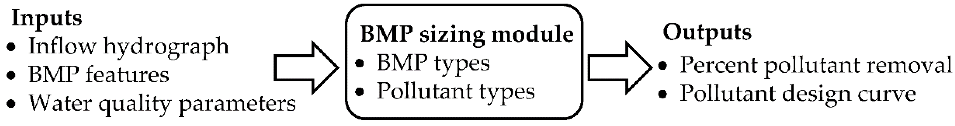
The conceptual framework of the water quality module within the i-DSTss tool is shown in Figure 1. Inputs into the water quality module include inflow hydrograph, BMP features and characteristics, and water quality parameters such as decay rate. Similar to the approach implemented in SUSTAIN [29], adsorption, settling, and filtration processes are lumped into one parameter, that is, decay rate.
The water quality module groups processes by BMP and pollutant type. Outputs from the water quality module include percent pollutant removal and pollutant design curve.
The water quality module is developed to calculate percent pollutant removal of BMPs based on the user-defined geometry and characteristics of BMPs. The sizing approach is different for infiltration-based BMPs and storage-based BMPs. In addition to the BMP types, the approaches implemented vary by pollutant type. The approaches used are summarized in Table 1 below. The water quality module includes 13 types of BMPs and 7 pollutants. BMP types are categorized in two different groups:
- (i)
- storage-based BMPs such as dry pond and wet pond,
- (ii)
- infiltration-based BMPs such as infiltration basin, dry well, infiltration trench, sand filter, porous pavement, grassed swale, vegetated filter strip, bioretention, rain garden, tree box, and wetland.
The functional relations between percent pollutant removal were developed based on mass balance. The details are presented in Section 2.2 and Section 2.3.
2.2. Infiltration-Based BMP Sizing According to Percent Pollutant Removal
The water quality module within i-DSTss allows up to seven pollutant types including colloids such as TSS and dissolved pollutants such as nutrients (total nitrogen (TN) and total phosphorous (TP)), metals, and bacteria such as Escherichia coli (E. coli) and fecal coliforms. A simplified colloid filtration theory (CFT) and decay rate approach have been implemented for the removal of colloids and dissolved pollutants, respectively.
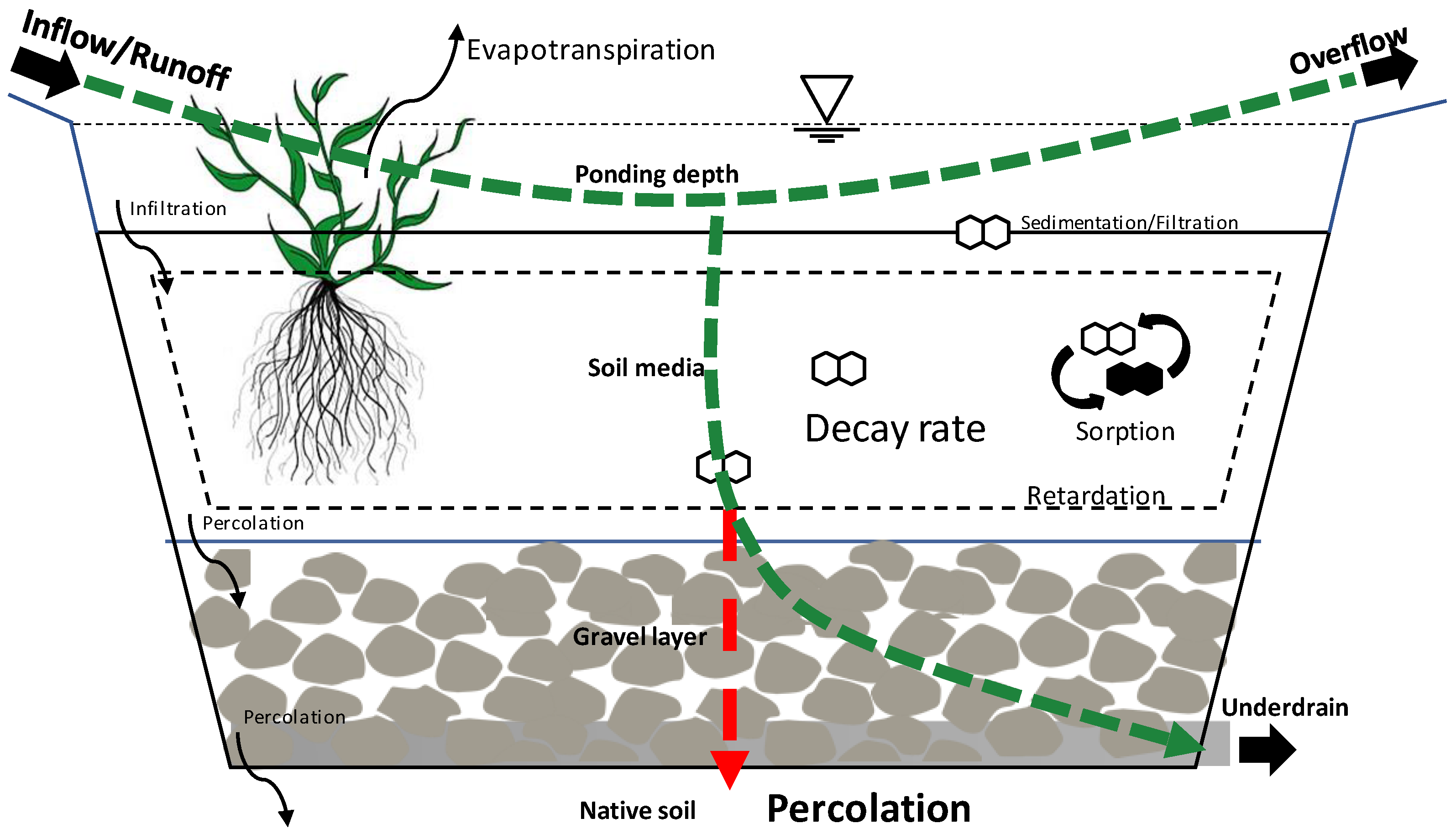
A conceptual diagram for pollutant removal processes in infiltration-based BMPs is shown in Figure 2. The number of layers vary in infiltration-based BMPs, with some BMP having three layers (a surface layer/ponding depth, a soil media layer, and a storage layer/gravel layer) and others with only a surface layer or a combination of surface layer with either soil media layer or storage layer [12]. When runoff enters infiltration-based BMPs, part of it becomes overflow and part of it percolates into the deeper soil and discharges via an underdrain. For the part that becomes overflow, percent pollutant removal is calculated in a similar way as for storage-based BMPs (presented later in Section 2.3.). For the part that discharges via the underdrain, percent pollutant removal is calculated based on decay rate and travel time in each layer. Finally, a combined efficiency is calculated based on concentration and proportion of overflow and underdrain amounts.
The combined removal efficiency for infiltration-based BMPs is given by Equation (1) as follows:
where Ec is combined efficiency, Ess is weighted average efficiency of soil media layer and storage/gravel layer, Es is efficiency of surface layer/ponding depth, QIN is runoff into an infiltration-based BMP in , and QOF is the overflow runoff out of an infiltration-based BMP in .
Removal efficiencies required in Equation (1) for the soil layer and storage layer can be calculated using Equations (2) and (4) separately. Then, a weighted average efficiency based on depth for both the soil layer and the storage layer is calculated. The approach used to calculate removal efficiency of surface layer is also similar to the methods developed for storage-based BMPs presented later in Section 2.4.
Default decay rate values are used for TP and E. coli for different types of BMPs. These values are changeable by the user and can be used for the calibration of the tool.
Equations (2) and (4) show the percent colloid and dissolved pollutant removal for infiltration-based BMPs as a function of BMP areas, respectively. Equation (2) is derived from colloid filtration theory [32,36] by simplifying interception and sedimentation terms, ignoring the diffusion term, and rearranging to solve for the percent colloid removal (details about BMP sizing approaches built into the water quality module are provided in Supplementary Materials). Equation (3) shows the interception transport mechanism and sedimentation transport mechanism terms used in Equation (2). Equation (4) is derived from the first-order decay reaction method [33] and was rearranged in a format to calculate the percent dissolved pollutant removal (details about BMP sizing approaches built into the water quality module are provided in Supplementary Materials).
where f is filter bed porosity, α is collision efficiency factor, n is single collector efficiency, z is filter bed depth in m, dp is median particle diameter in m, dc is collector diameter in m, ABMP is surface area of the BMP in m2, θ is water content, dmedia is depth of soil media in m, Q is runoff flow in , vs. is settling velocity in , and k is decay rate values in , QIN is runoff into a BMP in , and QOF is overflow runoff out of a BMP in .
2.3. Storage-Based BMP Sizing According to Percent Pollutant Removal
A similar approach was implemented for storage-based BMP types. Equations (5) and (7) show the percent TSS/colloid removal and percent dissolved pollutant removal for storage-based BMPs as a function of BMP size and flow characteristics. Equation (5) is derived from the ratio of settling velocity to critical velocity equation [35] and rearranged in a format to calculate the percent colloid removal (details about BMP sizing approaches built into the water quality module are provided in Supplementary Materials). Critical velocity is equal to the water flow rate into the pond divided by the pond surface area. A settling velocity greater than a critical velocity for a given particle size suggests that the particle is trapped before leaving the storage-based BMPs.
Equation (6) shows the equation for settling velocity, vs, [34] used in Equation (5). Equation (7) is derived from first-order decay [33] rearranged in a format to calculate the percent dissolved pollutant removal (details about BMP sizing approaches built into the water quality module are provided in Supplementary Materials).
where vs is the settling velocity in , D is the mean sieve diameter of grains in m, dBMP is the depth of the BMP in m, and QIN is runoff into a BMP in .
2.4. Performance Curve
Finally, the water quality module creates the BMP performance curve, and the BMP efficiency will be obtained from the performance curve. The performance curve is a curve in which BMP removal efficiency is graphed with respect to the sizing factor (the ratio of the area of the BMP to the area of the watershed). Relating the efficiency of the BMP to the size of the BMP and drainage area (described in detail in Supplementary Materials) assists the BMP design process [37]. Developing performance curves from the local climate provides a starting point to estimate actual reductions that could be achieved. Performance curves highlight the need to consider design parameters relative to total maximum daily load (TMDL) allocations (i.e., acceptable range for the watershed). Furthermore, these curves bracket the sensitivity of a range of assumptions for more significant parameters (e.g., surface area, infiltration rate) to evaluate potential BMP effectiveness [29]. The water quality module enables users to explore the tradeoff between the primary sizing (design criteria) and BMP performance by providing a performance curve.
3. Water Quality Module Test Cases—Performance Evaluation
To demonstrate the performance of the water quality module, measured water quality data were compared to simulated outputs for infiltration-based and storage-based BMPs. The details are presented in Section 3.1 and Section 3.2.
3.1. Infiltration-Based BMP
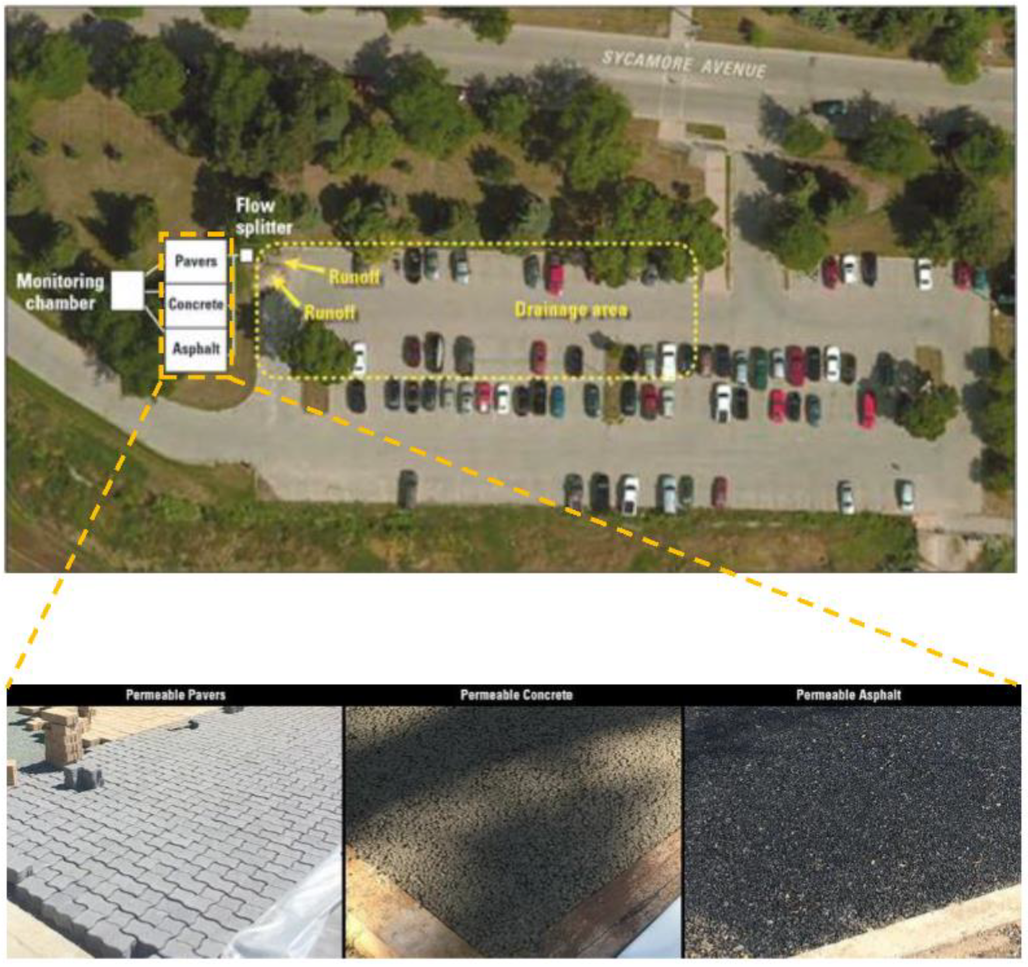
To demonstrate the performance of the water quality module, measured water quality data from a permeable pavement were used. A parking lot with an area of 1324 m2 in Madison, Wisconsin, drains into the permeable pavement located at the outlet of the parking lot. Figure 3 shows the parking lot and the permeable pavement. Inflow and outflow volumes were measured for different events [38]. A comparison of measured and simulated outflow volumes was presented by Shojaeizadeh et al. (2019) [12]. In this research, the fidelity of the water quality module was assessed based on comparison of simulated and measured percent pollutant removal for different types of pollutants including TSS, TP, and E. coli. Statistical evaluation techniques including R2 and the Nash–Sutcliffe coefficient of (NSE) were used as performance measures.
The total area of permeable pavement was 139.35 m2 consisting of three permeable pavement surfaces (permeable asphalt, permeable concrete, and permeable interlocking pavers) with equal area of 46.45 m2. The permeable pavement was developed for reducing runoff via infiltration and improving the quality of stormwater runoff originating from a conventional asphalt parking lot. Effluent water quality from the permeable pavement was compared with simulated outputs from the water quality module. A permeable pavement including each of the test plots is shown in Figure 3. The permeable pavement had a depth of approximately 50 cm. An impermeable membrane lining a sloped base (approximately 2 percent) was placed under the permeable pavement to collect and measure the infiltration rate. Actual removal efficiency was based on comparisons of the influent and effluent pollutant load for sampled events. Storm event loads at each monitoring location were computed by multiplying the EMC and event runoff volumes. Field and sample-processing equipment blanks were collected at all sample collection points, to evaluate the integrity of the water-quality sampling process, identify whether sample contamination existed and, if so, to identify possible sources [38]. Most of the available observed data were for the year 2015. We compared storm events from 2015 with the percent pollutant removal obtained from the water quality module. For each event, time series data were available for both precipitation and runoff. To make sure the results were accurate, volume of runoff into permeable pavement calculated using i-DSTss was compared with observed volumes before the start of comparing simulated water quality data with observed data.
Table 2 shows a list of parameters and their values used in the water quality module within i-DSTss for colloids and dissolved pollutants for the case study. Some are design variables and others are model parameters. Both design variables and model parameters can be changed by the user. Parameter values can be obtained from literature or determined by calibration (e.g., decay rate).
3.2. Storage-Based BMP
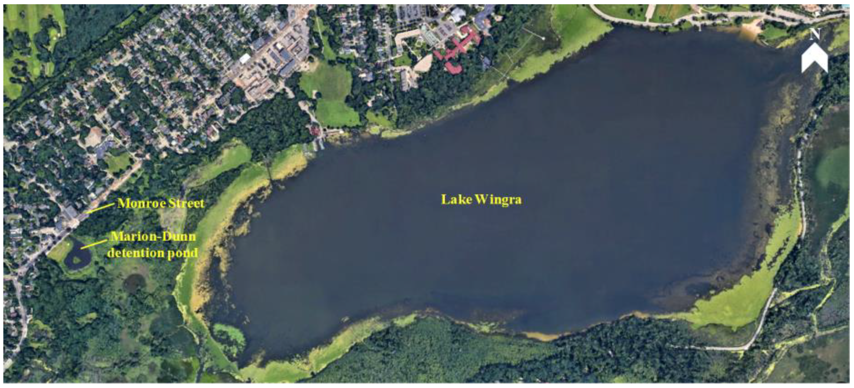
To demonstrate the performance of the water quality module, measured water quality data from a wet detention pond obtained from studies conducted by the U.S. Geological Survey (USGS) were used. The University of Wisconsin Arboretum in Madison, Wisconsin, constructed the Marion Dunn wet detention pond to protect the water quality and ecology of Lake Wingra from the effects of storm–sewer inflow to the lake (Figure 4). The Marion Dunn Pond is located on the downstream side of Monroe Street and the average basin slope is 2.2 percent. The pond has a surface area of 5670 m2, a maximum depth of 2.3 m, and an average depth of 1.1 m at normal pool elevation (Figure 4). It has a surcharge storage volume above the normal pool elevation that is capable of holding the 10-year, 24-h storm-runoff volume without overtopping. The pond has two outlets controlled by 45-degree V-notch weirs that drain to channels leading to Lake Wingra. The bottom of the pond consists of a clay layer that inhibits infiltration of water from or into the pond.
The Marion Dunn wet detention pond was monitored by the USGS to determine its effect on the water quality of urban runoff. The Marion Dunn Pond has a drainage area of 0.96 square kilometer, composed primarily of residential land use. TSS and TP event mean concentrations were determined from the detention pond inflow and outflow samples. EMC samples were collected for 64 runoff events. The data used for performance evaluation were not recent, however, the sampling techniques and analytical methods used are still valid. Thus, the data could still be used to conduct a valid comparison. Storm precipitation ranged from 1 to 51 mm during these events [39].
Table 3 shows a list of design and parameter values used in the water quality module for colloids and dissolved pollutants.
4. Results and Discussion
4.1. Performance Criteria
Many papers discussing the calibration of watershed models (e.g., [40,41]) use the coefficient of determination, R2, to measure the quality of calibration, which describes the degree of collinearity between simulated and observed values and varies from 0 to 1. R2 values greater than 0.5 are considered acceptable [42].
Although R2 has been widely used for model evaluation, this statistic is oversensitive to outliers and insensitive to additive and proportional differences between simulated values and observed data [43]. Hence, measures such as the Nash–Sutcliffe coefficient of efficiency (NSE) [44] and root mean square error (RMSE) are often considered to be more appropriate [45]. Thus, the NSE was also calculated. The limitation of NSE is that it does not include weighting, and thus ignores differences in uncertainty in observations [46]. NSE determines the model efficiency as follows:
where is observed data, is simulated values, and is observed mean data.
In this section, the results of two case studies including an infiltration-based BMP (permeable pavement) and a storage-based BMP (wet pond) are presented in Section 4.2 and Section 4.3, respectively.
4.2. Infiltration-Based BMP
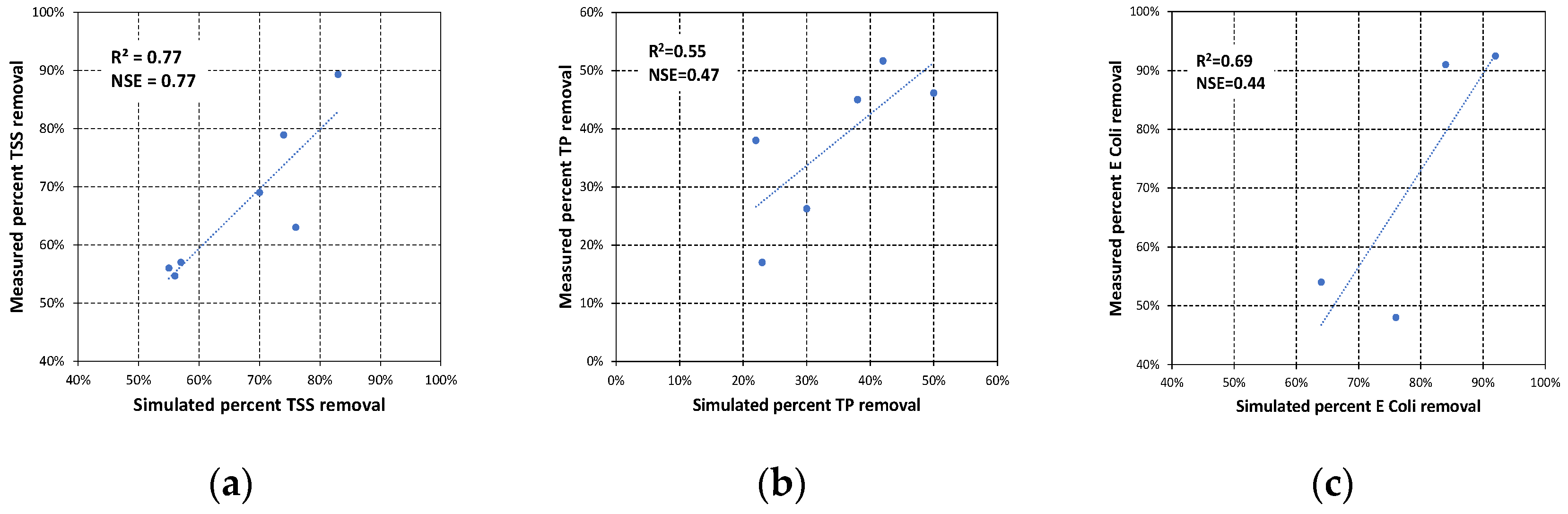
Percent TSS, TP, and E. coli removal from the water quality module were compared with observed data from a permeable pavement in Madison, Wisconsin. Table 4 shows precipitation values and antecedent dry time for different events.
Figure 5a compares percent TSS removal between observed data and simulated values for different events and shows the coefficient of determination, R2 and NSE, between observed and simulated values for all events. As shown in Figure 5a, both R2 and NSE are greater than 0.7, which is relatively good.
Figure 5b compares percent TP removal between observed data and simulated values for different events and shows the coefficient of determination, R2 and NSE, between observed and simulated values for six events (excluding event number 4) for which observed data were available. As shown in Figure 5b, both R2 and NSE are around 0.5, which is relatively acceptable.
Figure 5c compares percent E. coli removal between observed data and simulated values for different events and shows the coefficient of determination, R2 and NSE, between observed and simulated values for four events (excluding events number 2, 5, and 7) for which observed data were available. As shown in Figure 5c, R2 is 0.69 (relatively good) and NSE is 0.44 (relatively acceptable). Summarizing Figure 5a–c shows that the water quality module had better overall performance and prediction for percent TSS removal. The module had acceptable performance for percent TP and E. coli removal.
4.3. Storage-Based BMP
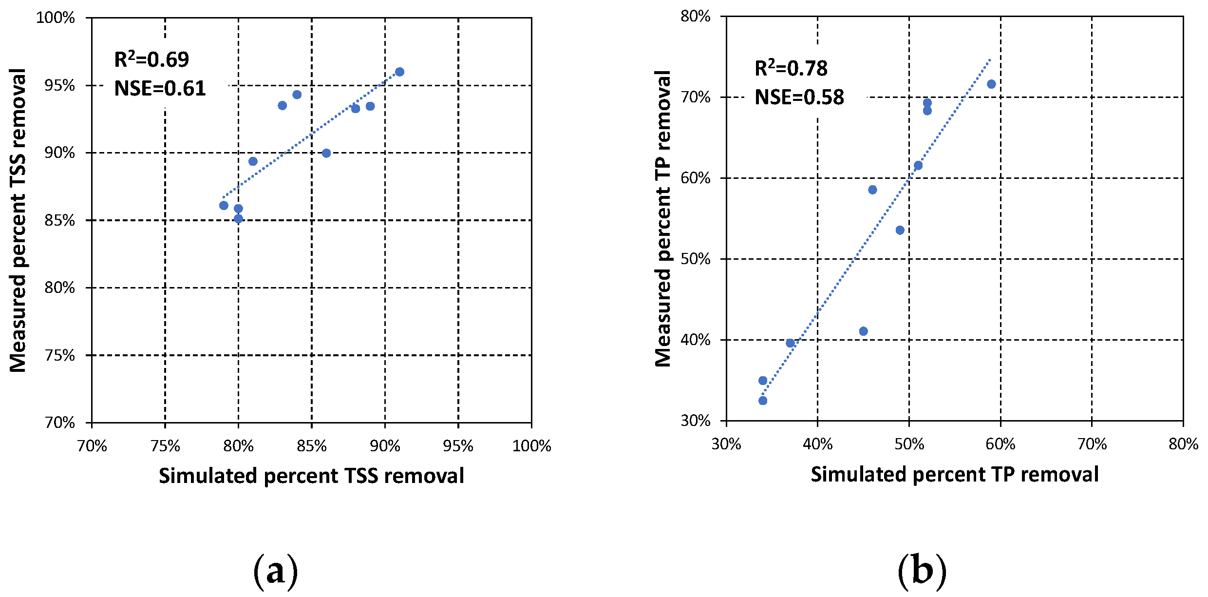
Simulated percent TSS and TP removal were compared with observed data for the Marion Dunn wet detention pond in Madison, Wisconsin. Table 5 shows precipitation values and antecedent dry time for different events.
Figure 6a compares percent TSS removal between observed data and simulated values for different events and shows the coefficient of determination, R2 and NSE, between observed and simulated values for all events. As shown in Figure 6a, both R2 and NSE are greater than 0.6, which is relatively good.
Figure 6b compares percent TP removal between observed data and simulated values for different events and shows the coefficient of determination, R2 and NSE, between observed and simulated values for all events. As shown in Figure 6b, R2 is 0.78 (relatively good) and NSE is 0.58 (relatively acceptable).
Summarizing Figure 6a,b shows that the water quality module had better overall performance and prediction for both of percent TSS and TP removal. The module had slightly better performance for percent TP removal. Additionally, the storage-based routines outperformed the infiltration-based routines at these two sites.
5. Conclusions
The water quality module is a part of the i-DSTss tool, which integrates several modules, including hydrology, BMP selection, BMP sizing, and cost. The water quality module includes sizing options for infiltration-based BMPs and storage-based BMPs. Decision-support tools in stormwater management become more useful to the users when they integrate multiple criteria and modules. Several factors were considered in the development of the water quality module within the i-DSTss including model accuracy, user interaction, and transparency. The water quality module employs a user interface that allows easy interaction; thus, it can be used by a wide range of users and designers who may not be modelers. The water quality module is relatively simple to implement, but equations for BMP performance and sizing are based on robust physically based, mass balance approaches.
To assess the fidelity of the tool, predictions from the water quality module were compared with observed data and the goodness-of-fit was evaluated for both BMP types including infiltration-based (a permeable pavement) BMPs and storage-based BMPs (a wet pond). The water quality module predicted BMP efficiency for three pollutant types including TSS, TP, and E. coli from a permeable pavement in Madison, Wisconsin. For percent TSS removal, both R2 and NSE values were greater than 0.7, demonstrating a good fit. For percent TP and E. coli removal, R2 and NSE values were around 0.5, demonstrating an acceptable fit. The water quality module also predicted BMP efficiency for two pollutant types including TSS and TP from the Marion Dunn wet detention pond in Madison, Wisconsin. For percent TSS removal, both R2 and NSE values were greater than 0.6, which is a relatively good fit. For percent TP removal, R2 is greater than 0.7 and the NSE value is greater than 0.5. A significant merit of the water quality module is that complex approaches were translated into easy to use, computationally less intensive, yet rigorous physically based modules that could be verified with observations. Due to the assumptions and simplifications made in the development, the tool has limitations. The physically based tool developed in this study may not be able to capture performance under complex environmental conditions. The tool does not account for the effect of temporal change in soil hydraulic properties due to physical or biological clogging or biogeochemical changes due to season. Future developments should consider the change in BMP efficiency over time. The tool does not include site-specific decay rate values. Future work should include testing the tool at different locations to develop site-specific values. However, the tool can generate better results than simplified empirical methods.
Supplementary Materials
The following are available online at https://www.mdpi.com/2073-4441/13/6/844/s1, A. Design procedure for different BMP group.
Author Contributions
Conceptualization, A.S., M.G., C.B., J.M., and T.H.; methodology, A.S. and M.G.; investigation, A.S. and M.G.; development, A.S.; writing—original draft preparation, A.S. and M.G.; writing—review and editing, A.S., M.G., C.B., J.M., and T.H.; supervision, M.G.; project administration, T.H. All authors have read and agreed to the published version of the manuscript.
Funding
This work was supported by the Environmental Protection Agency (EPA) (grant number EPA-G2015ORD-D1).
Institutional Review Board Statement
Study did not involve humans or animals.
Data Availability Statement
Study did not report any data.
Acknowledgments
We acknowledge William Selbig and USGS for sharing the hydrologic and water quality data of a permeable pavement and the Marion Dunn wet detention pond in Madison, Wisconsin.
Conflicts of Interest
The authors declare no conflict of interest.
References
- Bolstad, P.V.; Swank, W.T. Cumulative impacts of landuse on water quality in a southern appalachian watershed 1. J. Am. Water Resour. Assoc. 1997, 33, 519–533. [Google Scholar] [CrossRef]
- Mallin, M.A.; Johnson, V.L.; Ensign, S.H. Comparative impacts of stormwater runoff on water quality of an urban, a suburban, and a rural stream. Environ. Monit. Assess. 2009, 159, 475–491. [Google Scholar] [CrossRef]
- Wilson, C.; Weng, Q. Assessing surface water quality and its relation with urban land cover changes in the Lake Calumet Area, Greater Chicago. Environ. Manag. 2010, 45, 1096–1111. [Google Scholar] [CrossRef]
- Conway, T.M. Impervious surface as an indicator of pH and specific conductance in the urbanizing coastal zone of New Jersey, USA. J. Environ. Manag. 2007, 85, 308–316. [Google Scholar] [CrossRef]
- Gilvear, D.; Heal, K.; Stephen, A. Hydrology and the ecological quality of Scottish river ecosystems. Sci. Total Environ. 2002, 294, 131–159. [Google Scholar] [CrossRef]
- Hasan, M.S.; Geza, M.; Vasquez, R.; Chilkoor, G.; Gadhamshetty, V. Enhanced Heavy Metal Removal from Synthetic Stormwater Using Nanoscale Zerovalent Iron–Modified Biochar. Water Air Soil Pollut. 2020, 231, 1–15. [Google Scholar] [CrossRef]
- Hasan, M.S.; Geza, M.; Petersen, J.B.; Gadhamshetty, V. Graphene oxide transport and retention in biochar media. Chemosphere 2021, 264, 128397. [Google Scholar] [CrossRef] [PubMed]
- Parkinson, J. Drainage and stormwater management strategies for low-income urban communities. Environ. Urban. 2003, 15, 115–126. [Google Scholar] [CrossRef] [Green Version]
- McNett, J.; Hunt, W.F.; Davis, A.P. Influent pollutant concentrations as predictors of effluent pollutant concentrations for mid-Atlantic bioretention. J. Environ. Eng. 2011, 137, 790–799. [Google Scholar] [CrossRef]
- David, N.; Leatherbarrow, J.E.; Yee, D.; McKee, L.J. Removal efficiencies of a bioretention system for trace metals, PCBs, PAHs, and dioxins in a semiarid environment. J. Environ. Eng. 2015, 141, 04014092. [Google Scholar] [CrossRef] [Green Version]
- Ellis, J. Infiltration systems: A sustainable source-control option for urban stormwater quality management? Water Environ. J. 2000, 14, 27–34. [Google Scholar] [CrossRef]
- Shojaeizadeh, A.; Geza, M.; McCray, J.; Hogue, T.S. Site-Scale Integrated Decision Support Tool (i-DSTss) for Stormwater Management. Water 2019, 11, 2022. [Google Scholar] [CrossRef] [Green Version]
- Shojaeizadeh, A.; Geza, M.; Bell, C.; Gallo, E.; Spahr, K.; Hogue, T.; McCray, J. A Site Scale Integrated Decision Support Tool for Urban Stormwater Management. In World Environmental Water Resources Congress 2018: Water, Wastewater, and Stormwater; Urban Watershed Management; Municipal Water Infrastructure; and Desalination and Water Reuse; American Society of Civil Engineers: Reston, VA, USA, 2018; Volume 31, pp. 112–120. [Google Scholar]
- Birch, G.; Matthai, C.; Fazeli, M. Efficiency of a retention/detention basin to removecontaminants from urban stormwater. Urban Water J. 2006, 3, 69–77. [Google Scholar] [CrossRef]
- Vymazal, J.; Kröpfelová, L. Is concentration of dissolved oxygen a good indicator of processes in filtration beds of horizontal-flow constructed wetlands? In Wastewater Treatment, Plant Dynamics and Management in Constructed and Natural Wetlands; Springer: Berlin/Heidelberg, Germany, 2008; pp. 311–317. [Google Scholar]
- Mahmoud, A.; Alam, T.; Rahman, M.Y.A.; Sanchez, A.; Guerrero, J.; Jones, K.D. Evaluation of field-scale stormwater bioretention structure flow and pollutant load reductions in a semi-arid coastal climate. Ecol. Eng. X 2019, 1, 100007. [Google Scholar] [CrossRef]
- Peng, J.; Cao, Y.; Rippy, M.A.; Afrooz, A.; Grant, S.B. Indicator and pathogen removal by low impact development best management practices. Water 2016, 8, 600. [Google Scholar] [CrossRef]
- International Stormwater BMP Database. Developed by Wright Water Engineers, Inc. and Geosyntec Consultants for the Water Research Foundation (WRF), the American Society of Civil Engineers (ASCE)/Environmental and Water Resources Institute (EWRI), the American Public Works Association (APWA), the Federal Highway Administration (FHWA), and U.S. Environmental Protection Agency (EPA). 2018. Available online: http://www.bmpdatabase.org/download-master.html (accessed on 22 August 2018).
- Li, D.; Wan, J.; Ma, Y.; Wang, Y.; Huang, M.; Chen, Y. Stormwater runoff pollutant loading distributions and their correlation with rainfall and catchment characteristics in a rapidly industrialized city. PLoS ONE 2015, 10, e0118776. [Google Scholar] [CrossRef] [PubMed]
- Strecker, E.W.; Quigley, M.M.; Urbonas, B.R.; Jones, J.E.; Clary, J.K. Determining urban storm water BMP effectiveness. J. Water Resour. Plan. Manag. 2001, 127, 144–149. [Google Scholar] [CrossRef]
- Fassman, E. Stormwater BMP treatment performance variability for sediment and heavy metals. Sep. Purif. Technol. 2012, 84, 95–103. [Google Scholar] [CrossRef]
- Minnesota Pollution Control Agency. Quick Guide: MPCA Estimator Table Minnesota Stormwater Manual. 2015. Available online: http://stormwater.pca.state.mn.us/index.php/Quick_Guide:_MPCA_Estimator_tab (accessed on 28 March 2020).
- Minnesota Stormwater Manual, Overview of Minimal Impact Design Standards (MIDS); Minnesota Pollution Control Agency: Rochester, MN, USA, 2016.
- California State University Sacramento Office of Water Programs, California Phase II LID Sizing Tool Documentation Manual; California State University: Sacramento, CA, USA, 2019.
- Elliott, A.; Trowsdale, S.A. A review of models for low impact urban stormwater drainage. Environ. Model. Softw. 2007, 22, 394–405. [Google Scholar] [CrossRef]
- Wong, T.H.; Fletcher, T.D.; Duncan, H.P.; Jenkins, G.A. Modelling urban stormwater treatment—A unified approach. Ecol. Eng. 2006, 27, 58–70. [Google Scholar] [CrossRef]
- Rossman, L. Storm Water Management Model User’s Manual, Version 5.1 (EPA-600/R-14/413b); National Risk Management Research Laboratory, Office of Research and Development, US Environmental Protection Agency: Cincinnati, OH, USA, 2015.
- Moeini, M.; Shojaeizadeh, A.; Geza, M. Supervised Machine Learning for Estimation of Total Suspended Solids in Urban Watersheds. Water 2021, 13, 147. [Google Scholar] [CrossRef]
- Lee, J.G.; Riverson, J. SUSTAIN: Urban Modeling Systems Integrating Optimization and Economics. In Proceedings of the 50 years of Watershed Modeling Conference, Boulder, CO, USA, 23–26 September 2012; Available online: https://dc.engconfintl.org/watershed/23 (accessed on 28 March 2020).
- Shahin, M.; Maier, H.; Jaksa, M. Settlement prediction of shallow foundations on granular soils using B-spline neurofuzzy models. Comput. Geotech. 2003, 30, 637–647. [Google Scholar] [CrossRef]
- Pitt, R.; Maestre, A.; Clary, J. The National Stormwater Quality Database (NSQD, Version 4.02); Department of Civil and Environmental Engineering, University of Alabama: Tuscaloosa, AL, USA, 2018. [Google Scholar]
- Yao, K.-M.; Habibian, M.T.; O’Melia, C.R. Water and waste water filtration. Concepts and applications. Environ. Sci. Technol. 1971, 5, 1105–1112. [Google Scholar] [CrossRef]
- Tinoco, I.; Sauer, K.; Wang, J.C.; Puglisi, J.D.; Harbison, G.; Rovnyak, D. Physical Chemistry: Principles and Applications in Biological Sciences; Prentice Hall: Bergen County, NJ, USA, 1995; Volume 545. [Google Scholar]
- Wilson, B.; Barfield, B.; Moore, I.; Warner, R. A hydrology and sedimentology watershed model. Part II: Sedimentology component. Trans. ASAE 1984, 27, 1378–1384. [Google Scholar] [CrossRef]
- Chen, C.-N. Design of sediment retention basins. In Proceedings of the National Symposium on Urban Hydrology and Sediment Control, Lexington, Kentucky, 28–31 July 1975. [Google Scholar]
- Tiveron, T.; Gholamreza-Kashi, S.; Joksimovic, D. A USEPA SWMM Integrated Tool for Determining the Suspended Solids Reduction Performance of Bioretention Cells. J. Water Manag. Model. 2018. [Google Scholar] [CrossRef] [Green Version]
- Shojaeizadeh, A.; Geza, M.; Hogue, T.S. GIP-SWMM: A new Green Infrastructure Placement Tool coupled with SWMM. J. Environ. Manag. 2021, 277, 111409. [Google Scholar] [CrossRef]
- Selbig, W.R.; Buer, N. Hydraulic, Water-Quality, and Temperature Performance of Three Types of Permeable Pavement under High Sediment Loading Conditions; US Geological Survey: Reston, VA, USA, 2018.
- House, L.B.; Waschbusch, R.J.; Hughes, P.E. Water Quality of an Urban Wet Detention Pond in Madison, Wisconsin, 1987–1988; Wisconsin Water Science Center: Middleton, WI, USA, 1993.
- Anand, S.; Mankin, K.R.; McVay, K.A.; Janssen, K.A.; Barnes, P.L.; Pierzynski, G.M. Calibration and Validation of ADAPT and SWAT for Field-Scale Runoff Prediction 1. J. Am. Water Resour. Assoc. 2007, 43, 899–910. [Google Scholar] [CrossRef]
- White, K.L.; Chaubey, I. Sensitivity analysis, calibration, and validations for a multisite and multivariable SWAT model 1. J. Am. Water Resour. Assoc. 2005, 41, 1077–1089. [Google Scholar] [CrossRef]
- Santhi, C.; Arnold, J.G.; Williams, J.R.; Dugas, W.A.; Srinivasan, R.; Hauck, L.M. Validation of the swat model on a large rwer basin with point and nonpoint sources 1. J. Am. Water Resour. Assoc. 2001, 37, 1169–1188. [Google Scholar] [CrossRef]
- Legates, D.R.; McCabe Jr, G.J. Evaluating the use of “goodness-of-fit” measures in hydrologic and hydroclimatic model validation. Water Resour. Res. 1999, 35, 233–241. [Google Scholar] [CrossRef]
- Nash, J.E.; Sutcliffe, J.V. River flow forecasting through conceptual models part I—A discussion of principles. J. Hydrol. 1970, 10, 282–290. [Google Scholar] [CrossRef]
- Chu, T.; Shirmohammadi, A. Evaluation of the SWAT model’s hydrology component in the piedmont physiographic region of Maryland. Trans. ASAE 2004, 47, 1057. [Google Scholar] [CrossRef]
- Geza, M.; Poeter, E.P.; McCray, J.E. Quantifying predictive uncertainty for a mountain-watershed model. J. Hydrol. 2009, 376, 170–181. [Google Scholar] [CrossRef]
Figure 1.
Conceptual framework for water quality module.

Figure 2.
Conceptual diagram for pollutant removal processes in infiltration-based BMPs.

Figure 3.
Permeable pavement consisting of permeable asphalt, permeable concrete, and permeable pavers at the outlet of Parking lot located in Madison, Wisconsin [38].
Figure 3.
Permeable pavement consisting of permeable asphalt, permeable concrete, and permeable pavers at the outlet of Parking lot located in Madison, Wisconsin [38].

Figure 4.
Marion Dunn wet detention pond located in Madison, Wisconsin.

Figure 5.
Scatter diagram of observed and simulated values for (a) percent TSS removal, (b) percent TP removal, and (c) percent E. coli removal.
Figure 5.
Scatter diagram of observed and simulated values for (a) percent TSS removal, (b) percent TP removal, and (c) percent E. coli removal.

Figure 6.
Scatter diagram of observed and simulated values for (a) percent TSS removal and (b) percent TP removal.
Figure 6.
Scatter diagram of observed and simulated values for (a) percent TSS removal and (b) percent TP removal.


Table 1.
Sizing approaches for different best management practice (BMP) groups by pollutant types.
| BMP Group | Pollutant Removal Approach | Reference | |
|---|---|---|---|
| Colloids | Dissolved Pollutant | ||
| Infiltration-based | Simplified CFT | Decay rate | Yao et al. (1971) [32] and Tinoco et al. (1995) [33] |
| Storage-based | Settling | Decay rate | Wilson et al. (1984) [34], Chen et al. (1975) [35], and Tinoco et al. (1995) [33] |
CFT, colloid filtration theory.
Table 2.
List of parameters and their values used in the water quality module by pollutant type.
| Parameters | Colloids | Dissolved Pollutant |
|---|---|---|
| Values | Values | |
| Surface area (m2) | 46.45 | 46.45 |
| Soil/paver depth (cm) | 15.24 | 15.24 |
| Storage depth (cm) | 40.64 | 40.64 |
| Saturated moisture content (%) | 0.45 | 0.45 |
| Decay rate (1/day) | - | TP: 0.25 * |
| Escherichia coli: 2.0 | ||
| QIN(m3/s) | Calculated for each event | Calculated for each event |
| QOF(m3/s) | ||
| Ponding depth (cm) | 0 | 0 |
| dc(mm) | 0.1 | - |
| dp(mm) | 0.02 | - |
| α | 0.5 | - |
| f | 0.5 | - |
* SUSTAIN model [29] suggests 0.2/day. TP, total phosphorus.
Table 3.
List of design variables and parameter values used in the water quality module by pollutant type.
Table 3.
List of design variables and parameter values used in the water quality module by pollutant type.
| Variable/Parameters | Colloids | Dissolved Pollutant |
|---|---|---|
| Values | Values | |
| Surface area (m2) | 5670 | 5670 |
| Average depth (m) | 1.1 | 1.1 |
| Decay rate (1/day) | - | TP: 0.25 * |
| QIN (m3/s) | Calculated for each event | Calculated for each event |
| D (mm) | 0.02 | - |
* SUSTAIN model [29] suggests 0.2/day.
Table 4.
Storm event number, precipitation volume, and antecedent dry time.
| Event Number | 1 | 2 | 3 | 4 | 5 | 6 | 7 |
|---|---|---|---|---|---|---|---|
| Precipitation (mm) | 7 | 9 | 46 | 14 | 15 | 12 | 6 |
| Antecedent dry time (days) | 9 | 1 | 12 | 3 | 9 | 9 | 24 |
Table 5.
Storm event number, precipitation volume, and antecedent dry time.
| Event Number | 1 | 2 | 3 | 4 | 5 | 6 | 7 | 8 | 9 | 10 |
|---|---|---|---|---|---|---|---|---|---|---|
| Precipitation (mm) | 18 | 15 | 43 | 8 | 51 | 21 | 19 | 12 | 29 | 20 |
| Antecedent dry time (days) | 5 | 9 | 4 | 1 | 6 | 5 | 2 | 7 | 9 | 4 |
Publisher’s Note: MDPI stays neutral with regard to jurisdictional claims in published maps and institutional affiliations. |
© 2021 by the authors. Licensee MDPI, Basel, Switzerland. This article is an open access article distributed under the terms and conditions of the Creative Commons Attribution (CC BY) license (http://creativecommons.org/licenses/by/4.0/).
Share and Cite
MDPI and ACS Style
Shojaeizadeh, A.; Geza, M.; Bell, C.; McCray, J.; Hogue, T. A Site-Scale Tool for Performance-Based Design of Stormwater Best Management Practices. Water 2021, 13, 844. https://doi.org/10.3390/w13060844
AMA Style
Shojaeizadeh A, Geza M, Bell C, McCray J, Hogue T. A Site-Scale Tool for Performance-Based Design of Stormwater Best Management Practices. Water. 2021; 13(6):844. https://doi.org/10.3390/w13060844
Chicago/Turabian StyleShojaeizadeh, Ali, Mengistu Geza, Colin Bell, John McCray, and Terri Hogue. 2021. "A Site-Scale Tool for Performance-Based Design of Stormwater Best Management Practices" Water 13, no. 6: 844. https://doi.org/10.3390/w13060844
Note that from the first issue of 2016, this journal uses article numbers instead of page numbers. See further details here.