
Tidal Oscillation and Resonance in Semi-Closed Estuaries—Empirical Analyses from the Elbe Estuary, North Sea
by
 , ,
, ,
Sebastian S. V. Hein
1,*, 
Vanessa Sohrt
1,
Edgar Nehlsen
1,
Thomas Strotmann
2 and
Peter Fröhle
1 1
Institute of River and Coastal Engineering, Hamburg University of Technology, 21073 Hamburg, Germany
2
Hamburg Port Authority, Hydrology, 20457 Hamburg, Germany
*
Author to whom correspondence should be addressed.
Water 2021, 13(6), 848; https://doi.org/10.3390/w13060848
Submission received: 4 March 2021
/
Revised: 12 March 2021
/
Accepted: 15 March 2021
/
Published: 19 March 2021
(This article belongs to the Special Issue Hydrodynamics in Estuaries and Coast: Analysis and Modeling)
Abstract
:Many tidal influenced estuaries and coastal basins feature tidal amplification because of, e.g., convergence and reflection. Increasing amplification rates were observed in the Elbe estuary, with consequences for construction measures, nautical manoeuvring, flood protection, riverbed morphology and ecosystems. Although many studies were conducted investigating the tidal wave transformation in estuaries, studies based on spatially well-distributed empirical data covering periods over more than a year are rare. To fill this gap, a self-developed adapted harmonic analysis method of least squares was applied to hydrographs from 25 gauges, distributed over the tidal influenced estuary from the river mouth to the tidal border which is given by the weir 160 km upstream of the river mouth. The investigation period for the harmonic analyses covers a whole nodal cycle of 18.613 a beginning in the year 2000. The tidal constituents’ oscillatory behaviour including the appearance of compound tides, generated by nonlinear shallow water processes, and the formation of reflection induced partially standing waves are determined. The tidal constituents show shared frequency-group specific partial clapotis, but also have significant differences in amplification within those groups. The latter fact contributes to the detected inverse proportionality of tidal range amplification inside the estuary to incoming tidal wave height. As reflection can cause resonance in tidal influenced rivers, tests are developed to analyse whether criteria for resonance are met. To determine the system’s specific resonance frequency, a new method was introduced with the three-parameter Lorentzian curve-fitting. As the detected resonance frequency is not close to tidal frequencies, full-established resonance of the tidal wave and of the tidal constituents is not observed in the Elbe estuary. Migrating nodes of the partially standing tidal wave hint at increasing latent resonance.
1. Introduction
Various estuaries and coastal basins exhibit extreme tidal conditions compared to their adjoining open sea because of system internal tidal wave transformation. Causes are often convergence and wave reflection. Tidal waves that fulfil the critical ratio of system length to tidal wavelength of approximately 1/4 (quarter-wavelength criterion, which is also known as resonance criterion) further frequently increase tidal ranges. In this case, the natural period of the oscillating system equals the exciter period of the tidal wave and resonance occurs [1]. An example is the Bay of Fundy in the west of Nova Scotia (Canada), where a fulfilled quarter-wavelength criterion causes tidal ranges more than 12 m, in extreme cases more than 16 m [1,2,3,4]. Over the last century, an increasing number of tidal rivers and basins, e.g. Thames [5], Scheldt [6], Ems [7], Elbe [8], showed a critical evolution of tidal wave transformation, primarily associated with conducted river engineering measures. In the Elbe estuary, the tidal range doubled from 1.9 m to 3.8 m since 1880 in the port of Hamburg, while the tidal range at the river mouth 100 km downstream stayed nearly constant around 2.9 m. The aggravation of tidal conditions can have severe consequences for the system’s morphodynamics, sediment budgets, stratification and consequently ecology, construction measures, flood protection and nautical manoeuvring. To cope with these difficulties in the Elbe, yearly water way maintenance costs running into tens to hundreds of millions for operators. However, there is still a lack of comprehension of the tides’ oscillatory behaviour in estuarine systems, although numerous studies have been conducted.
Examples of previous works on tidal waves in estuaries are the publications by Aubrey and Speer [9,10], who analysed the non-linear tidal propagation of tides in shallow inlets and estuaries. Their studies are based on observations of surface elevation and horizontal currents in the Nauset inlet (Orleans) covering periods ranging from three days to one year and a one-dimensional numerical model. Even so, only nine gauges for the large branching inlet and periods of only up to one year were considered, conclusions could be drawn and clarified by their model: An establishing tidal asymmetry inside the inlet with shorter but stronger floods and consequently a net sediment import into the inlet were observed. Overtides (higher harmonics) and compound tides, increasing in amplitude inside the estuary, were identified as the cause. Van Rijn [11] conducted analytical and numerical model-based analyses of tidal wave propagation in funnel-shaped estuaries. Modelled channels were 60 km to 290 km long, were based on the estuaries of the rivers Scheldt (Netherlands), Hooghley (India) and Delaware (USA) and covered microtidal to macrotidal, shallow to deep and smooth to rough bottom roughness conditions. They state that amplification due to convergence dominates dissipation due to bottom friction in deep channels and vice versa in shallow channels. Further they say that reflection against the landward end of a closed channel is important in the most landward 1/3 of the total channel length.
Regarding previous studies in the Elbe, Eichweber and Lange [12,13] analysed current data from 14-days of measurements by 75 sensors distributed over the estuary focussing on the principal tide M2 with its higher harmonics and their effects on sediment dynamics. The authors assume that the quarter-wavelength criterion for resonance [1] is met in the Elbe estuary. They state that this resonance amplifies the M2’s higher harmonic M6 and that the main dredging sites coincide with the nodes of M2’s higher harmonics’ standing waves. Consequently, river engineering measures should consider designs to dissipate these harmonics. Rolinski and Eichweber [14] further compared the results from the velocity measurements to a hydrodynamical model. They declared that the existence of standing waves is indicated by amplitudes and phases derived from measured and simulated velocity data, but the influence of standing waves on suspended particulate matter dynamics could not be proved. More recently, Backhaus [15] and Hartwig [16] investigated tidal oscillation behaviour in the Elbe estuary regarding possible occurring resonance based on models, using a simplified geometry. They interpreted the increasing tidal ranges as an indicator of an increasing latent resonance (near resonant state), originating from conducted water way deepenings [8]. Backhaus determined a natural resonance period of the Elbe estuary to be 15.37 h, which is significantly lower than Hartwig’s estimated natural resonance period of 20.5 h.
The present studies are part of the German Coastal Engineering Research Council (KFKI) project RefTide, a collaboration between the Hamburg Port Authority (HPA) and the Hamburg University of Technology (TUHH). The aim is the determination of the recent status quo of tidal oscillation and tidal resonance of the Elbe estuary. We present a detailed analysis of the tidal constituent specific oscillatory behaviour in an estuary, for the first time according to our findings, based on water level measurements covering the whole estuary in a high spatial resolution (average gauge distance: 7 km) and a whole nodal cycle of 18.613 a of minutely data. The high spatial resolution of digital water-level data in the tidal influenced Elbe estuary, dating back beyond the year 2000, allows for extensive analyses of tidal oscillations including tidal reflection and resonance. We prove the existence of partially standing waves, after their formation was previously hinted by the velocity measurements analysed by Eichweber, Lang and Rolinski [12,13,14]. Differences in extent of amplification between tidal constituents of similar frequency are detected and the possible causes such as shallow water constituents and consequences for tidal range evolution inside the estuary are discussed. The used self-programmed harmonic analysis method of least squares (HAMELS) considers nodal modifications directly in the multiple regression, which has the advantage over conventional tools that it can distinguish between principal and shallow water constituents sharing a common frequency. To advance conventional analyses of tidal resonance, two new innovative approaches are presented and applied to the Elbe estuary. Based on the investigations presented, future studies can be conducted to investigate the temporal development of the tidal oscillations and the influencing factors.
2. Materials and Methods
2.1. Study Site
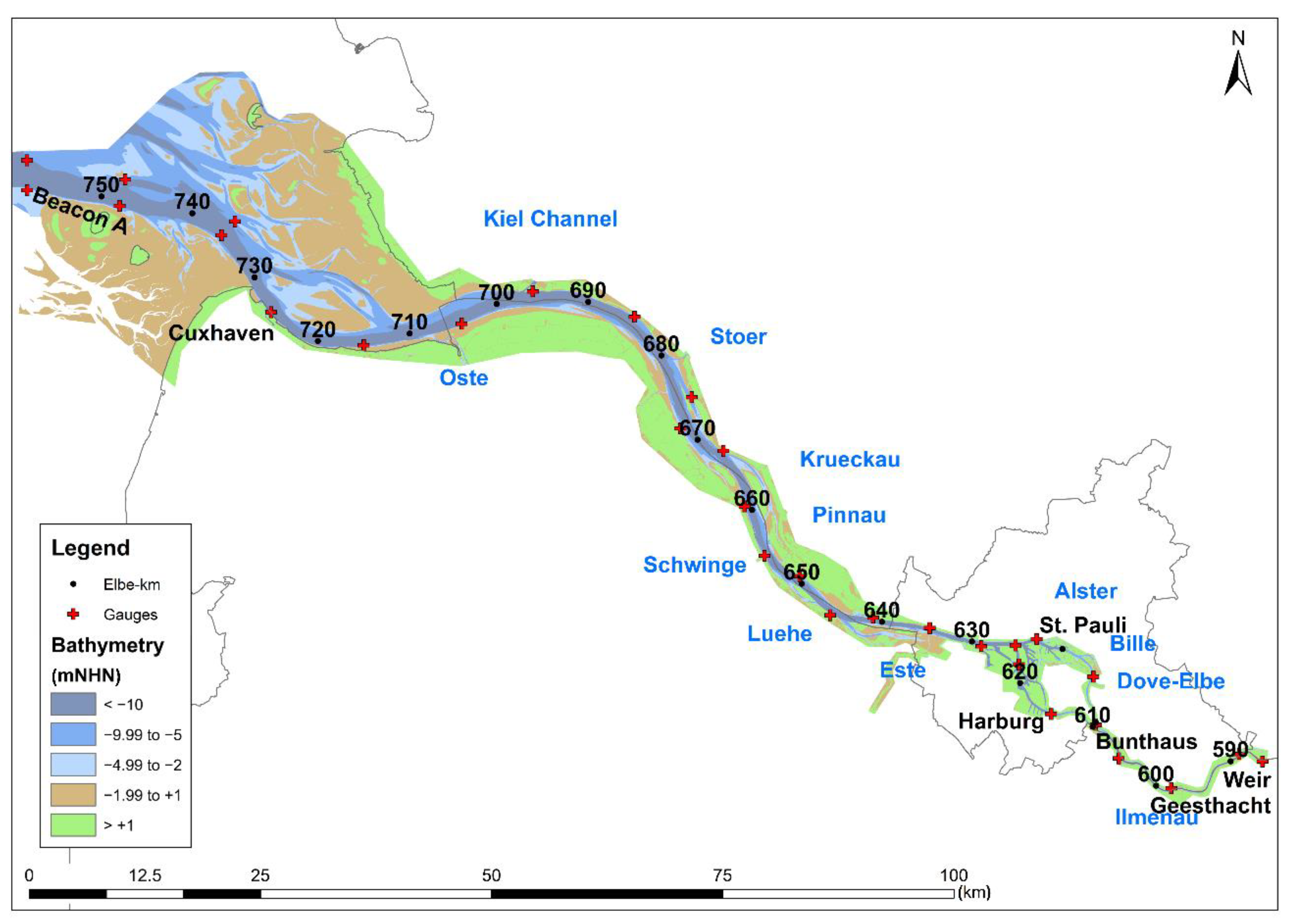
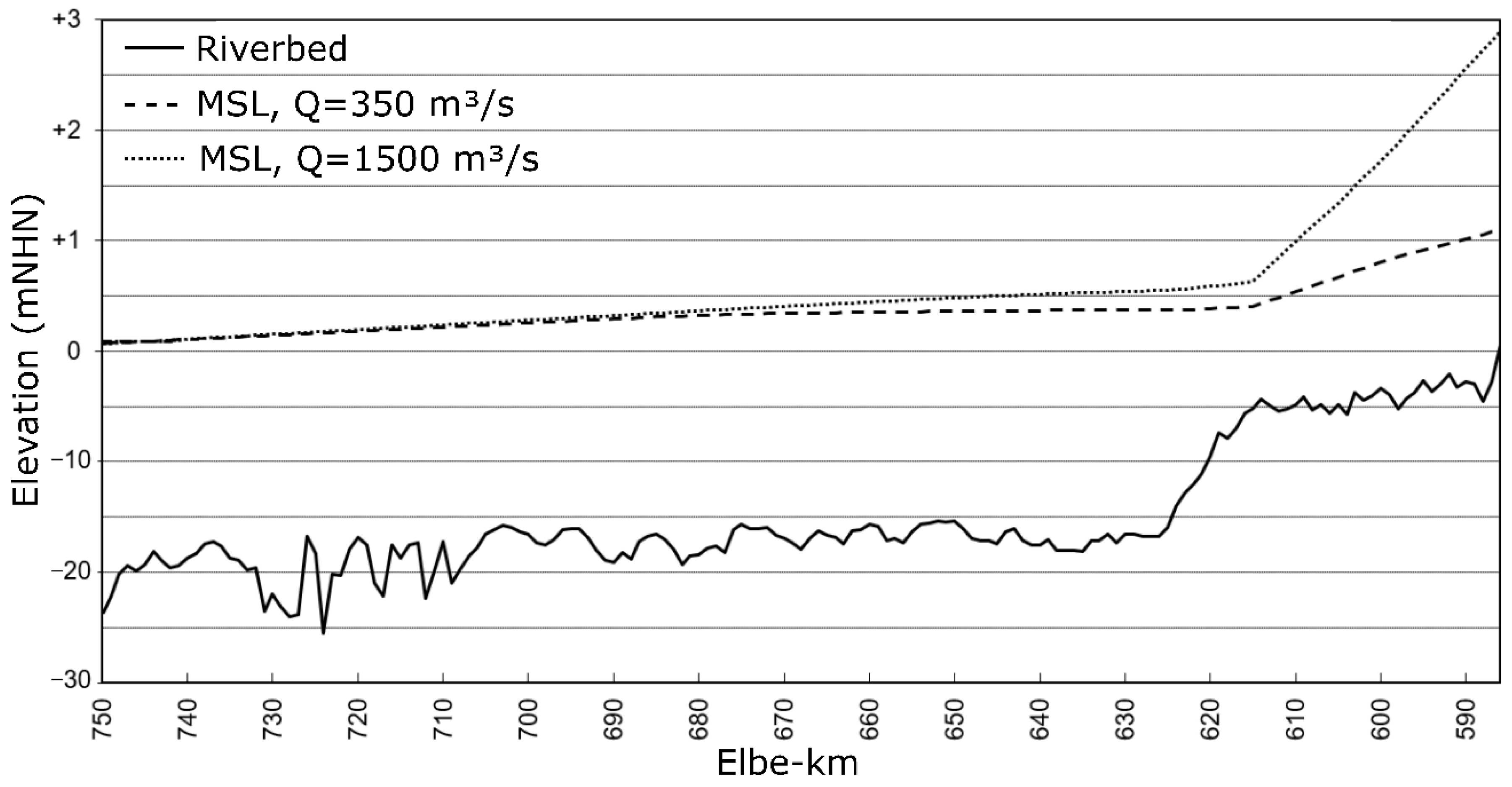
The Elbe estuary opens into the German Bight of the North Sea where tidal ranges are mostly mesotidal between 2 m and 4 m. Wind conditions are dominated by westerly winds, mainly from 247.5° to 315°. The Elbe estuary (Figure 1) reaches from its river mouth between Cuxhaven (southern bank, Elbe-km 724) and Friedrichskoog (northern bank) up to the weir in Geesthacht (Elbe-km 586). The weir is the artificial limit of the tide in the estuary, except during storm surges when it is set. The upper Elbe estuary between the weir Geesthacht (Elbe-km 686) and gauge Bunthaus (Elbe-km 610) is mostly less than 10 m deep (Figure 2) and has a width of 300 m to 500 m. Between Bunthaus and river kilometre 626, the Elbe is branched into the Northern and Southern Elbe. The Northern Elbe is between 200 m and 400 m wide and has a bathymetric change in depth at Elbe-km 620 from −6 mNHN (german Normalhöhennull; above the base height level) upstream to −17 mNHN downstream. The Southern Elbe is 200 m to 300 m wide and has a similar bathymetric change at Elbe-km 615. The lower Elbe between Elbe-km 626 to 724 at Cuxhaven has water depths between −16.6 mNHN and −25 mNHN. At Elbe-km 633, the Lower Elbe estuary widens from 500 m to 2.5 km at high tide and 1.5 km at low tide. The river mouth widens between Elbe-km 695 and 724 to a width of 17.5 km. Outside the river mouth, the fairway runs 30 km through the Wadden Sea [8].
Major tidal wave reflection occurs in the Elbe estuary mainly at the abrupt bathymetric changes in the Southern Elbe at river kilometre 615, in the Northern Elbe around kilometre 620 and at the weir in Geesthacht at Elbe-km 586. The cross-sectional constrictions are partial reflectors and the weir is a total reflector. The maximal tidal ranges are measured at the partial reflectors around river kilometre 615 in the Southern Elbe. Minimal tidal ranges are between Elbe-km 675 and 695. Upstream the cross-sectional constrictions, the tidal range decreases, as a result of increased bottom friction, as the water depth is lower and because of the increased damping influence of the river discharge in this area. These dissipative influences predominate the theoretical total reflection induced amplification at the weir. Entering the Elbe estuary, the tidal wave shows an almost sinusoidal form. As the wave progresses upstream, the waves’ flood gradient becomes steeper and the ebb gradient flattens, along with decreasing flood tide duration towards the upstream while the ebb-tide duration increases. An increasing river discharge influence towards the weir additionally contributes to the wave form deformation. The river discharge into the Elbe estuary is recorded at the gauge Neu Darchau (Elbe-km 536.44). The most important characteristic values of the discharge are for the time series from 2000 to 2018:
- Mean discharge: 674 m3/s.
- Modal value: 371 m3/s.
- Lowest observed discharge: 162 m3/s (16 August 2015).
- Mean lowest annual discharge: 254 m3/s.
- Days with discharge <350 m3/s: 1452.
- Highest observed discharge: 4080 m3/s (11 June 2013).
- Mean highest annual discharge: 2153 m3/s.
- Days with discharge >1500 m3/s: 447.
The 30-year running mean of river discharge into the Elbe estuary decreased over the last decades from 741 m3/s in 1990 to 692 m3/s in 2000 to 649 m3/s in 2019, with a constant low from 2014 to 2019 with a mean discharge of 487 m3/s [17]. Elbe discharges feature seasonal variation. Between 2014 and 2019 the mean discharge from November to April was 643 m3/s and 334 m3/s from May to October. The mean sea level (MSL) for discharges of 350 m3/s and 1500 m3/s are shown together with the fairway bathymetry in Figure 2. The influence of the discharge on the MSL gradient is mainly limited to the upper part of the estuary between the cross-sectional constrictions around Elbe-km 620 and the weir. Between the entry of the estuary and the port of Hamburg where the partial reflector is located, the MSL differences are only 25 cm to 30 cm at 350 m3/s discharge and 50 cm to 60 cm at 1500 m3/s over a distance of more than 100 km. For more details and illustrations reference is made to previous studies by Boehlich and Strotmann [8,18,19].
2.2. Materials
Data basis for the harmonic analysis is the digital water-level data collected every minute by 25 gauges distributed over the Elbe estuary from the outer river mouth up to the tide limiting weir in Geesthacht. Gauge’s operators and data provider are the Waterways and Shipping Offices of Lauenburg (Elbe-km 686–605), Hamburg (Elbe-km 639–690) and Cuxhaven (Elbe-km 690–755) and the Hamburg Port Authority (Elbe-km 605–639). The raw data can be accessed at www.kuestendaten.de. A low-pass filter with a cut-off frequency of 1/30 min was applied to the raw data, to attenuate nontidal waves. For the harmonic analyses, a temporal resolution of 60 min was used.
2.3. Tidal Analysis Methods
For the tidal spectral analyses, a self-programmed harmonic analysis method of least squares (HAMELS) was used. This HAMELS-tool features some advantages over conventional tools:
- The exact angular positions of all considered tidal constituents including their nodal corrections are calculated for every data point, which increases the accuracy.
- Nodal corrections are directly considered in the multiple regression in the HAMELS, improving the correctness of the calculated amplitudes and phases. Further, it enables to distinguish between principal and shallow water constituents sharing a common frequency.
The momentary angular positions of tidal constituents were calculated as described, e.g., by Schureman [20]. The tidal constituents’ angular frequencies are composed of periodical solar and lunar elements (Table 1): mean longitude of sun h(t), longitude of solar perigee p’(t), mean longitude of moon s(t), longitude of lunar perigee p(t) and longitude of moon’s node N(t). The composition of every tidal constituent is given by its Doodson number [21]. Those solar and lunar elements can be calculated from five orbital parameters: the mean elongation of the moon D(t), the mean anomaly of the sun M(t), the mean anomaly of the moon M’(t), the mean argument of perigee F(t) and the mean longitude of the Moon’s ascending node Ω(t). Those orbital parameters were calculated for every point in time of the data points following the Standards of Fundamental Astronomy (SOFA) provided by the International Astronomic Union (IAU) [22].
Nodal corrections are necessary in tidal analyses as they take the lunar modification into account, which alternates the tidal potential forces over an 18.613 a cycle (detailed explanations in Schureman [20] and Parker [23]). While the node factor f is multiplied with the amplitude and varies around 1, the phase correction u has to be added to the angular position and ranges around 0. The nodal correction parameters f and u were determined for each individual time stamp of the data points, following the calculation principle of Schureman [20] (derivations of the six underlying correction elements ξ, ν, ν’, ν”, R and Q for the phase correction are described in his chapters 24, 25, 131 and 132). Taking the inclination of the moon’s orbit to the celestial equator I into account, the node factor f can be calculated after Schureman’s Equations (65)–(80), (141)–(150), (215), (227) and (235) [20]. The node factor f of a compound tide is the product of the node factors of the interfering primary tidal constituents. The nodal phase modulation u is received by the addition and subtraction congruent to the calculation of a compound tides frequency as described by the International Hydrographic Organisation [24]. The used nodal correction parameters were validated via a comparison to the nodal correction parameters after the International Hydrographic Organisation [24].
In shallow waters, tidal waves are affected by nonlinear processes (detailed explanation in Parker’s chapters 2.3.2 and 7.6 [23]). Their effects become revealed by an increasing asymmetry of the tidal wave. The increasing nonlinearity is accompanied by an energy transfer from the principal tides to their higher harmonics (also called overtides) and from interfering principal tides to newly generated shallow water compound tides. They can have the same Doodson number/mean frequency as astronomical principle tidal constituents. An example is the S2 and the shallow water compound tide KP2, both having an average period of 12 h. As nodal corrections are directly applied in our HAMELS, it is possible to distinguish two tidal constituents with identical Doodson numbers, as the singularity of functions in the multiple regression is not violated: S2 has no nodal correction and consequently a theoretically constant amplitude and angular frequency ω of 2 cycles per day (cpd), while the KP2 has both a nodal amplitude and phase correction. Consequently, the different node factors and phase corrections in the functions ensure, that the singularity of functions is satisfied. The actual angular frequency differs during all time points, except when u is 0, or if both tidal constituents on a common frequency have a phase correction, when both u-values are equal. When analysing a duration that is at least 18.613 a long, the Rayleigh-criterion is met for frequency deltas larger than 0.00014709 cpd allowing for differentiations between those tidal constituents. In the case of the M2 and KO2 just 0.13% of the hourly datapoints does not fit the Rayleigh-criterion. In the case of the S2 and the KP2, it is even less with 0.06%.
Our HAMELS uses multiple linear regression to solve the data series for all considered sinusoidal tidal constituents, whose frequencies must be given. For the harmonic analysis we chose up to 97 tidal constituents, for all of them, the amplitudes and local phase φ, given for the common point in time 1 January 2000 12:00:00 UTC, were calculated for which the residual sum of squares is minimal. The residuals are the deviations between the original measured hydrograph and the reconstructed hydrograph, utilising the determined tidal constituent parameters. Those deviations result, as not all hundreds of tidal constituents can be considered, of which many have less than a centimetre in amplitude and because of non-astronomical influences on the tidal curve, such as meteorological effects. The detailed mathematics of the harmonic analysis method of least squares is well explained in the manual by Boon III and Kiley [25]. Our HAMELS was validated via a comparison of the evaluated tidal constituents of measured water level data from the Elbe with established MATLAB Toolboxes, such as UTide, which was devised by Codiga [26].
2.4. Resonance Tests
A short introduction into the quarter-wavelength criterion for tidal resonance in coastal waters is given and two innovative resonance tests for determination of a system’s resonance frequency and variations of latent resonance are presented in the following:
Full resonance occurs in a freely oscillating system when the exciter period Te equals the resonance (or natural) period Tr of the system. The resonance period of a simplified semi-closed basin/channel of equal width and depth with a total reflector at its closed end depends on the gravitational acceleration , its length l and depth d:
where the term in denominator equals the wave velocity c according to the linear wave theory (Airy) which applies to tidal waves in shallow waters where depths d are less than a twentieth of the wavelength L:
The period Te of a tidal wave acting as the exciter with a wavelength can be calculated via Equation (3):
Consequently, the exciter and resonance frequencies are equal when the length of the basin is a quarter of the tidal wavelength:
If this condition is met, the node of the establishing (partially) standing wave lies at the open end at the river mouth, the antinode with maximal amplitudes is located at the reflector and the system’s eigen oscillation and the forced exciter oscillation are synchronous. This condition is often referred to as quarter-wavelength criterion or quarter-wavelength resonance and is elucidated in more detail by Proudman [1]. This criterion can be expanded to further conditions of unequal multiples of a quarter for the ratio, since also in these cases a second, third (and so on) node is located at the open end and inner and outer oscillation are in sync [27]:
Subsequently, deduced resonance tests were developed and applied. In the first approach, a three-parameter Lorentzian curve-fitting (LCF) is used to estimate the estuaries resonance frequency. An LCF can generally be used to describe or estimate the shape of a resonance curve [28] and is also used in other scientific fields to estimate resonance frequencies, for example electrical science [29]. In freely oscillating systems, the amplification increases with closeness to the resonance frequency. Consequently, an LCF over the amplification values of the tidal constituents of different frequencies is assumed to indicate the resonance frequency corresponding the fitting curve’s maximum. The LCF function is defined as
where A is the height of the peak frequency, x0 the position of the peak frequency, x the position of each frequency and γ is the half width at half height [28]. The parameters must be roughly estimated previously to the fitting. Here start parameters after Betzler [30] were used:
where y is the amplification value of each frequency,
The node of the (partially) standing wave in a semi-closed opened system is located at the open end in the case of full established resonance. Therefore, the locations of the node for the hydrological years (example 2000: 1 November 1999–31 October 2000) 2000 to 2019 are used in the second approach to analyse if the oscillatory system got closer to a resonating status, meaning increasing latent resonance. For this purpose, a four-term Fourier model (Equation (10)) for a curve-fitting over the yearly mean tidal ranges of the gauges between the outer river mouth at beacon A (Elbe-km 755.6) and the antinode at the main reflector (Elbe-km 620) are used to locate the minimum tidal range, which indicates the node. In the Fourier series, is the intercept, ai and bi are the coefficients to be determined, x is the position and is the signal’s fundamental frequency.
The slope of the regression line through the river kilometre positions over the respective year then gives out the mean migration rate of the node.
3. Results and Discussion
Tidal constituents can be grouped, depending on their frequency, into long-period, diurnal, semidiurnal and 1/n-diurnal tides [21]. This study focusses on the diurnal, semidiurnal, quarter-diurnal and sixth-diurnal tidal species, as they tend to bear the most energy [31]. For the resonance test using the LCF, also the eighths-diurnal constituents were considered, to test the quarter-wavelength criterion for the system-to-wavelength ratio of 5/4. A general overview of tidal constituent specific oscillations in tidal reflection exhibiting estuaries and the Elbe estuary specific status quo of tidal oscillations between 2000 and 2018 is provided. The analyses were applied to a whole nodal cycle (1 January 2000 13:00:00 CET to 13 August 2018 00:00:00 CET) between the fairway deepenings in 1999/2000 and 2020/2021. During those times no further deepening measures were conducted.
3.1. Group Specific Oscillations
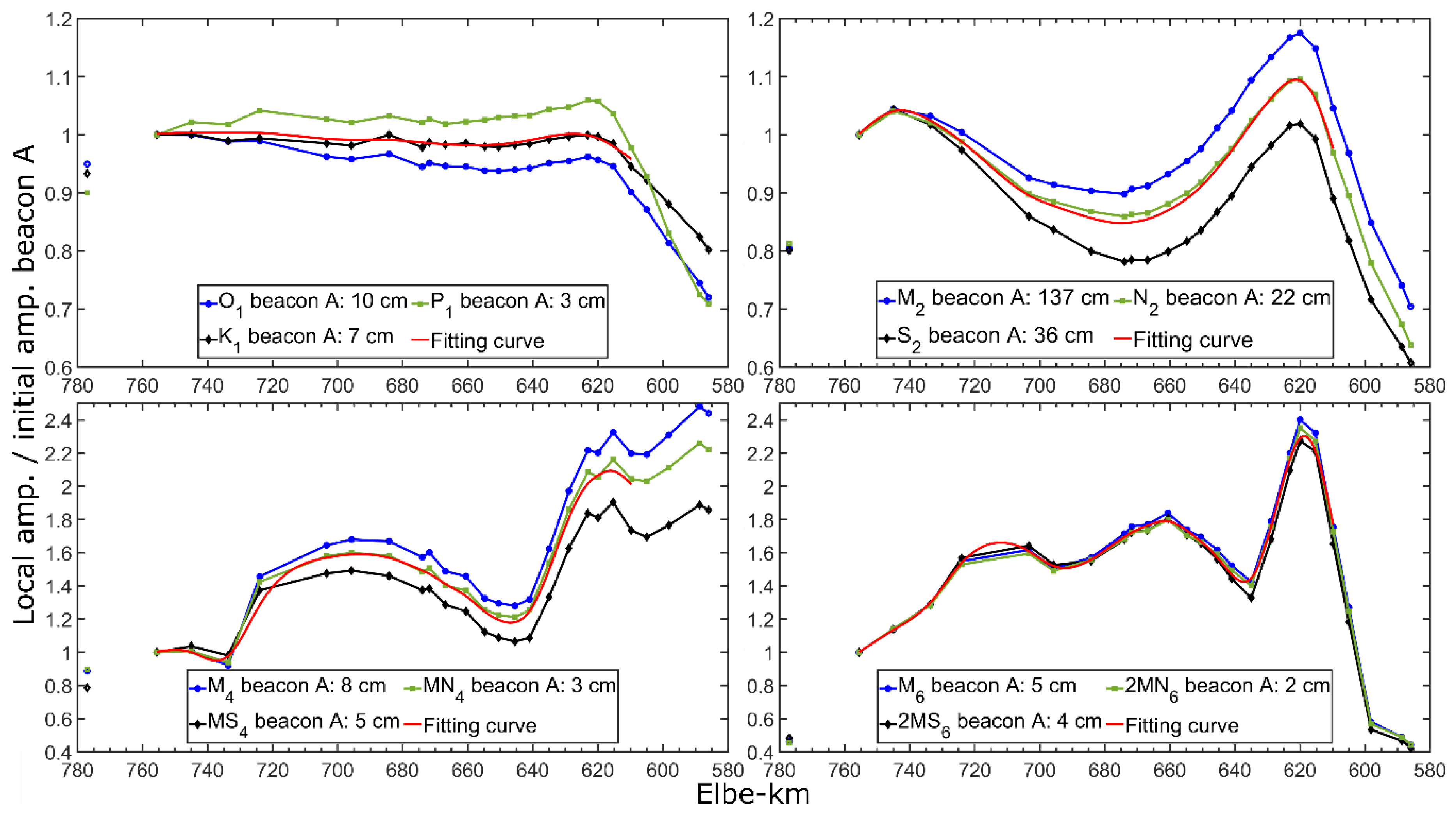
The harmonic analyses of 18.613 years of data from 25 gauges in the Elbe estuary indicate that each tidal frequency group has its own specific oscillatory behaviour as illustrated by the calculated amplitudes plotted against the gauge locations in the Elbe (Figure 3). The waveforms show a distinct reflection influence. Diurnal tides commonly show approximately constant amplitudes along the Elbe estuary with just one weakly-marked antinode with its maximum at the partial reflectors. Upstream of the partial reflector the amplitudes steadily decrease. Semidiurnal to sixth-diurnal tides show prominent formations of partial clapotis (standing waves) with distinct nodes and antinodes. All frequency groups show an antinode at the partial reflector, whereby the number of antinodes in the lower Elbe estuary increases with the species index: The semidiurnal tides oscillate in form of an uninodal partial clapotis, quarter-diurnal tidal constituents in a binodal partial clapotis and the sixth-diurnal tidal constituents suggest a trinodal partial clapotis, whereby the third node perishes in the decreasing trend towards the open sea. Consequently, the distance between the (anti)nodes decreases with the species index. As the wave speed c in shallow water solely depends on water depth d, all tidal constituents must theoretically propagate with the same speed. When the wave speed stays the same, but the frequency doubles, the wavelength must consequently halve, which is approximately the case. Quarter and sixth-diurnal tides amplify inside the estuary about twice as much as the semidiurnal tides. The loss in energy of the semidiurnal tides to higher frequencies upstream the estuary comes along with an increasing nonlinearity of the superimposed tidal wave with steeper flood gradients and flatter ebb gradients [8], conforming the observations of Aubrey and Speer [9,10]. A phenomenon that is only prominent in the quarter-diurnal species is the further increase in amplitude upstream of the partial reflector to Elbe-km 589, although the river discharge strongly dampens the superimposed tidal wave in this part of the estuary and other species decrease rapidly.
The observed tidal constituent specific partial clapotis are consistent with observations by Redfield [32], who analysed superimposed tidal waves in tidal driven embayments. According to Redfield [32], the node lies outside the system, if the length of a bay is shorter than 1/4 of the driving tidal wavelength, and the amplitude increases towards the head of the bay. If the bay is longer than 1/4 of the tidal wavelength, nodes appear inside the bay, as occurring in the Elbe estuary. The existence of partial clapotis are further supported by the findings of Eichweber and Lange [12,13] who conducted harmonic analysis based on spatially well distributed current hydrographs from the ELBEX measuring campaign in 1992. They detected standing wave patterns, but these could not be confirmed by models [14]. Together with this work, both current velocity data and measured water levels now prove the existence of standing waves. Furthermore, the partial clapotis extend across and significantly influence the entire estuary and not just the most landward 1/3 of the estuary, as stated by van Rijn [11] for estuaries covering microtidal to macrotidal, shallow to deep and smooth to rough bottom roughness conditions and lengths of 60–290 km. Concerning potential phase jumps during reflection, Hartwig [16] deduces from a 2D-numerical Elbe estuary model that no significant phase jumps would occur at the reflectors in the Elbe estuary.
The further increase in quarter-diurnal tidal amplitudes upstream the reflector indicates that the stronger influence of fluvial counter currents in this part increase the energy transfer to quarter-diurnal tidal constituents and thus increases the nonlinear asymmetry of tidal waves. Such an increase in asymmetry can be observed in the Elbe estuary [19]. Consequently, the semidiurnal tidal constituents especially lose in dominance in the uppermost part of the tidal influenced river. Analyses of current data (not shown here) confirm these observations: M4/M2 amplitude ratios of current velocity increases with increasing discharge and dependency ratios increase with closeness to the weir. These observations are supported by Parker [33], who also observed increasing M4/M2 amplitude ratios with increasing discharge in a numerical model of the Delaware River and Bay, USA. Studies from Hunt [34] also outline a decreasing dominance of semidiurnal tidal constituents in the uppermost part of the Thames estuary, Great Britain.
3.2. Group Internal Variations and Compound Tides
Although the frequency groups show common partial clapotis forms, group internal differences between tidal constituents were observed regarding degree of amplification. The two most energetic tidal constituents M2 and S2 differ remarkably (Figure 3). S2 is significantly less amplificated than the M2, even though their frequencies differ by only 0.0677 cpd. A first likely reason for this observation is the momentum conservation, but the results imply that the degree of amplification inside the Elbe estuary does not solely depend on the incident amplitude height: The highest amplitude does not always show the highest degree of amplification and the lowest amplitudes never show the lowest amplification. Another reason for a lesser amplification of the S2 in comparison to the M2 is the quadratic friction: Two interfering tidal constituents, such as the M2 and S2, which causes the Spring-Neap-Cycle, go in and out of phase over a cycle, whose period is the reciprocal of the frequency delta (in this example 14.77 d). When both tidal constituents are in phase, the tidal range and consequently also the currents are enhanced. As the energy dissipation due to quadratic friction is proportional to the square of the current speed, the mean amplitudes of both constructively interfering tidal constituents are smaller than they would be without the other tidal constituent. Herein, the relative damping of the lower tidal constituent S2 is greater than the one of the higher tidal constituent M2, as the relative current speed increase is greater [23].
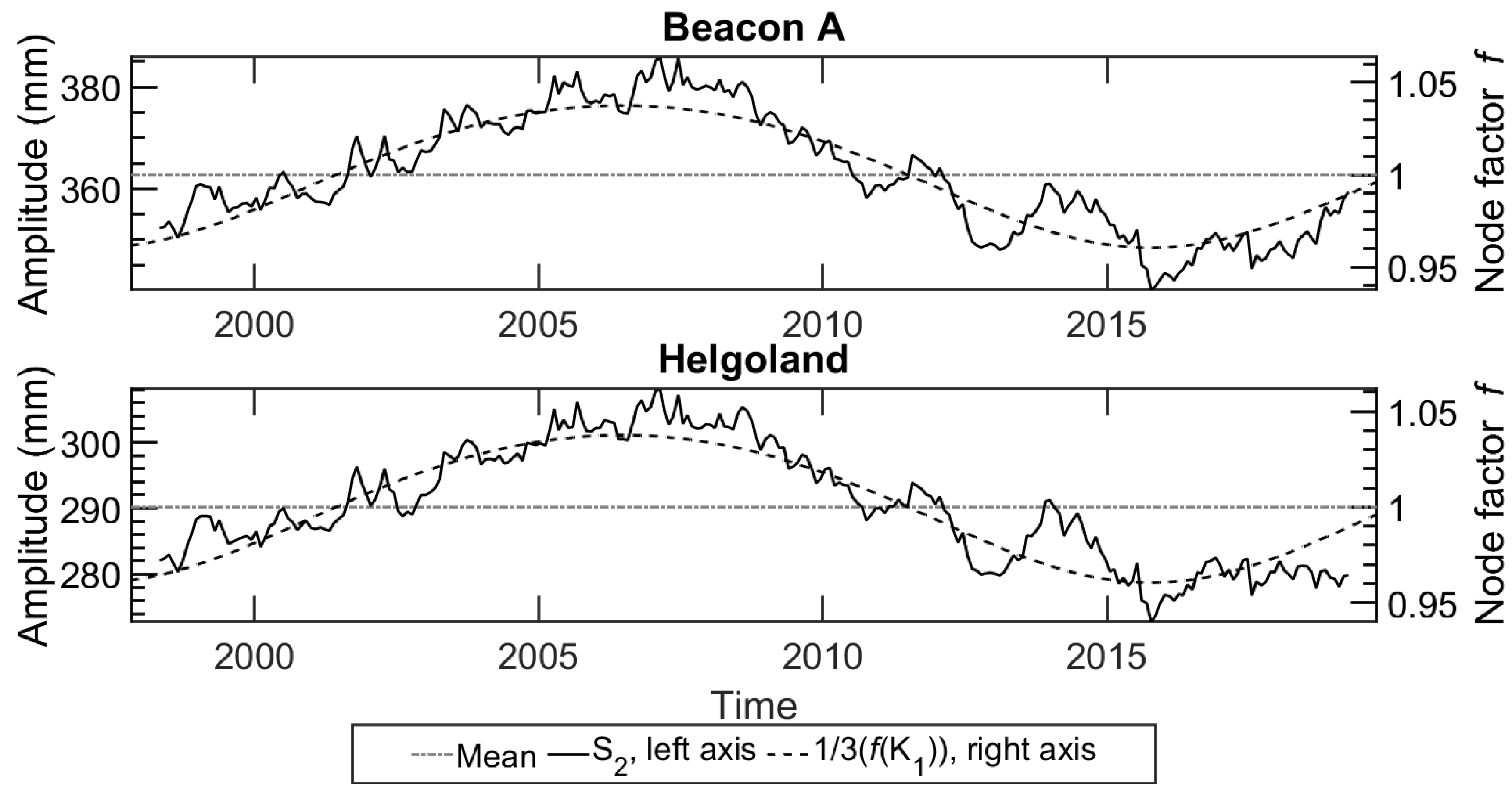
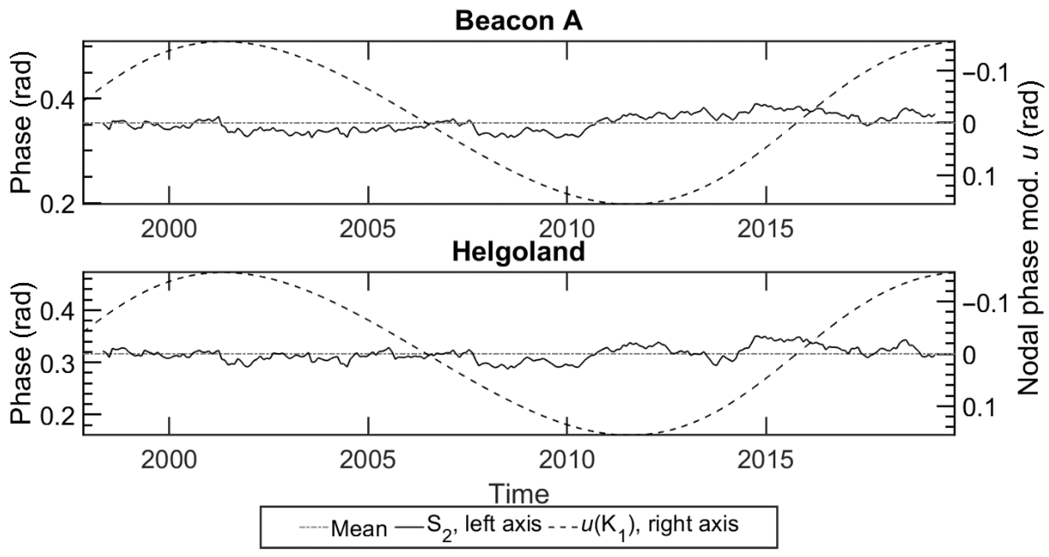
To analyse further reasons for the different amplifications of close tidal frequencies in oscillatory systems alike the Elbe estuary, it has to be considered that an astronomically given frequency cannot be occupied by only one, but by additional shallow-water compound tides. A proof for the existence of multiple tidal constituents on the same frequency delivers an analysis of the S2 at the gauge beacon A located in the outer river mouth and gauge Helgoland in the German Bight (Figure 4). As the S2 is a purely solar tidal constituent, it has no nodal correction. Yet, stepwise harmonic analyses over 365.25 days shifted by two Spring-Neap cycles (29.5 days) over 22 years show a periodic amplitude variation over a nodal cycle. This observation can be attributed to the shallow water compound tide KP2 on the same mean frequency with its nodal correction. The KP2 is the compound tide of K1 and P1. As P1 is a solar tide and has no nodal corrections, f and u of KP2 equals f and u of K1 [24]. The observed amplitude variation on the shared 2-cpd frequency matches 33% of f(K1), hinting that a third of the energy can be attributed to the compound tide. However, the phase does not follow the nodal phase correction of the KP2 but indeed stays almost constant, despite some minor fluctuations (Figure 5). Two HAMELS applied to a whole nodal cycle of 18.613 a, one with activated nodal amplitude and phase correction and one with only activated amplitude correction were conducted (singularity of functions is not violated, as node factors differ). The analyses with both corrections result in KP2 to S2 amplitude ratios of 42:325 mm (11.4% KP2) at gauge beacon A and 35:257 mm (12% KP2) at gauge Helgoland. If only the amplitude correction is activated, the KP2 to S2 amplitude ratios to 146:236 mm (38% KP2) at gauge beacon A and 104:193 mm (35% KP2) at gauge Helgoland. The latter case better conforms the observed 33% of K1 modulation. Furthermore, fast-Fourier transformations of the residuals reveals that an artificial satellite constituent at frequency S2 (2 cpd) plus N (0.0001 cpd) is generated when also the phase correction is activated, whereas the analysis with only the nodal amplitude modulation can explain the energy in this frequency band completely. Those results further demonstrate that not just inside the estuary and at the coast shallow water compound tides are generated, but also in the German Bight, where water depths are greater as they reach up to 56 m.
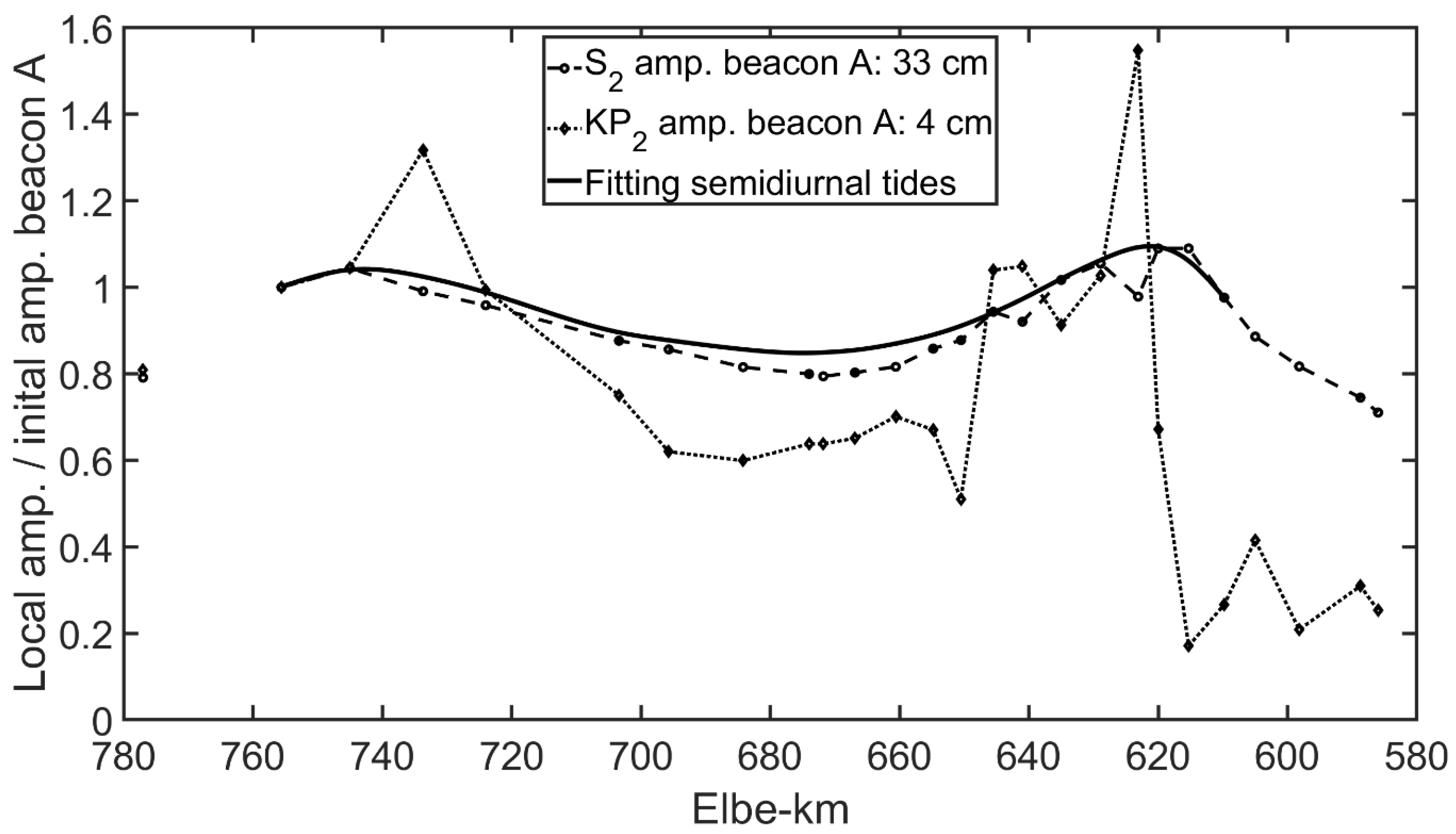
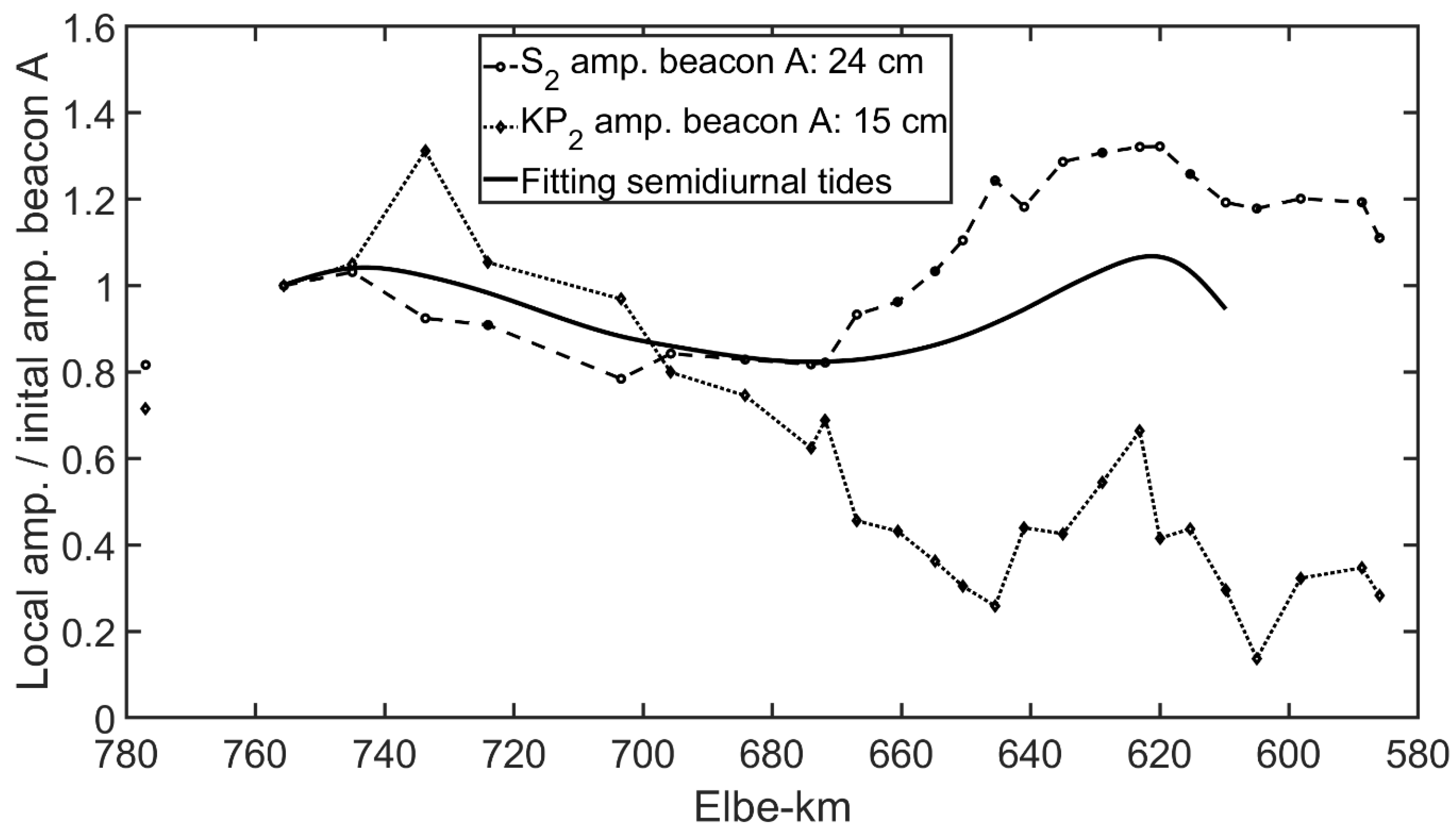
As the principal tides share their frequencies with shallow water compound tides, the source of differences in amplification could also lie in the compound tides. We keep the example of the S2 and KP2. The KP2 results from nonlinear energy transfer from the diurnal tides K1 and P1 and thus eventually could have a less semidiurnal typical partial clapotis form without the high amplification at the reflector but a more diurnal curve form. Thus, a possible reason for the lesser amplification of the shared S2 and KP2 frequency in comparison with the M2 and KO2 frequency could be the observed higher energy share of the KP2 11.4% in comparison to the KO2 share of 8% (calculated for beacon A with activated f and u correction). If both amplitude and phase corrections are activated one might interpret a decreasing trend of the KP2 upstream the Elbe estuary, but the relative amplification follows the shape of a semidiurnal tide with its two antinodes and the amplification at gauge STP is even higher than the amplification of the S2 (Figure 6). Note that S2 and KP2 are not in phase, but the difference is just 43.26° at Elbe-km 620, where the KP2 amplitude is maximal, thus the interference is still constructive. However, if just the nodal amplitude modulation of the KP2 is considered, the KP2 amplitude along the estuary shows a significant decrease (Figure 7). The S2 amplitude is significantly more amplified at the reflector. Consequently, these results could explain at least a share of the lesser S2 amplification in comparison to the M2 when no shallow water compound tides are considered (Figure 3). However, so far, we cannot explain why the amplitude on the shared S2 and KP2 frequency is apparently partly modulated by the KP2’s node factor but does not show any KP2’s phase modulation.
These determined differences in amplification have direct consequences: they cause, for example, decreasing amplification inside the estuary with increasing incoming tidal ranges. The dependency of the estuarine tidal amplification at the gauge St. Pauli (STP) in the port of Hamburg on incoming tidal ranges from the German Bight, measured at Helgoland, is illustrated in Figure 8. This dependency is partly attributed to the quadratic friction, as higher tidal ranges cause greater tidal currents and thus higher dissipation. A calculation of the tidal ranges resulting from the interference of the Spring-Neap-Cycle causing principal tides M2 and S2 shows that also for the lesser amplification of S2, the amplification of the tidal range inside the estuary is lesser during spring tides than neap tides (Table 2).
3.3. Resonance Tests
To analyse whether an estuary is affected by resonance, the test of the quarter-wavelength criterion is usually applied. As real wavelengths and system lengths are usually not as trivial to determine as for simplified channels, two additional derived approaches were developed and applied to the Elbe estuary.
3.3.1. Quarter-Wavelength Criterion
The open seaward end of the Elbe estuary is assumed to be between the end of the maintained waterway at Elbe-km 755 and Cuxhaven at Elbe-km 724 (e.g. by Hartwig [16]) where the river mouth opens into the Wadden Sea. The landward end of the tidal influence is the weir in Geesthacht at river kilometre 586. The maximal amplification occurs at the abrupt bathymetric changes in the port of Hamburg around Elbe-km 620 in the Northern Elbe and 615 in the Southern Elbe. Thus, for the application of the quarter-wavelength criterion, this reflector is assumed to be the landward end of the oscillation system in which the partially standing wave is developed. Depending on chosen ends, the length of the oscillatory system ranges between 105 km and 170 km. Determined semidiurnal wavelength in the Elbe estuary calculated via multiple approaches including different effective water depths in Equation (3), calculated phase velocities, observed run-times and hydrodynamic-numerical modelling vary between 337 km and 500 km. Considering these system lengths and tidal wavelengths, the quarter-wavelength criterion can be either rejected or confirmed. Backhaus [15] assumed a system length of 130 km and wavelengths of 408 km and 452 km, utilising effective water depths of 8.5 m and 10.5 m, respectively. Backhaus [15] and Hartwig [16] state that no full resonance is established, but latent resonance occurs, contributing to the tidal ranges in the port of Hamburg. Eichweber and Lange [13] state that the quarter-wavelength criterion is met for the Elbe estuary, without giving tidal wavelengths and system lengths. However, the node in the Elbe estuary lies in between Elbe-km 685 and 695, which cannot be considered the seaward end, and consequently the quarter-wavelength criterion is not fulfilled.
3.3.2. Lorentzian Fit
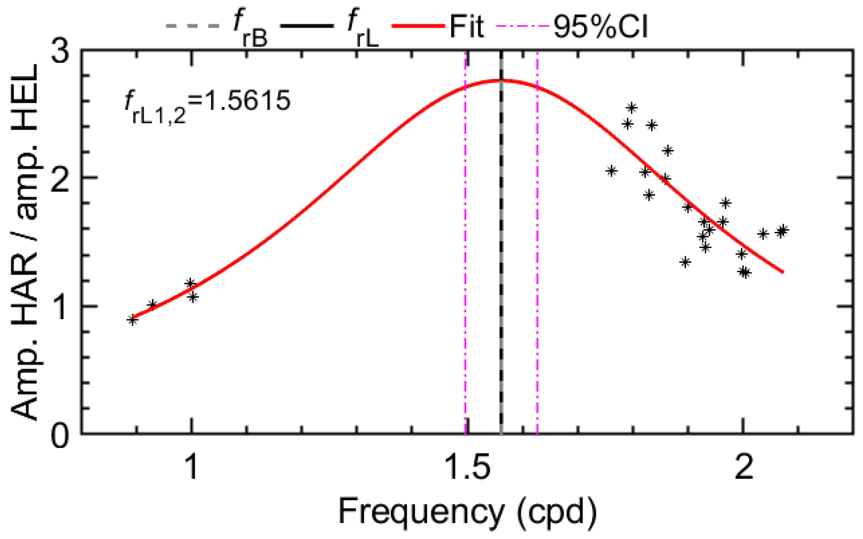
The tidal constituent analysis with its determinable tidal constituent specific amplification enables an additional approach to specify the resonance frequency of an estuary. The resonance frequency fr is assumed to be between the diurnal and semidiurnal frequency band. The amplification factors of the analysed diurnal and semidiurnal tidal constituents between the gauge Helgoland and Harburg at the abrupt bathymetric change in the Southern Elbe (Elbe-km 615) show that an increased amplification with closeness to such a resonance frequency is not consistent, but a tendency can be observed (Figure 9). After applying the LCF function, the maximum amplification ratio gives an approximation of the resonance frequency, in this case 1.5615 cpd (Tr = 15.37 h). Due to the naturally given frequency gap between diurnal and semidiurnal tides and because factors such as friction can alter the shape of a system specific resonance curve [32], the calculated resonance frequency should be treated with care. To validate this method, a comparison with previously determined resonance frequencies of the Elbe estuary in studies by Backhaus [15] and Hartwig [16] was conducted. Following Backhaus (2015), the resonance frequency of the recent Elbe estuary is 1.5615 cpd (Tr = 15.37 h), which exactly coincides with the determined resonance frequency. After Hartwig [16] the resonance frequency is with 1.171 cpd (Tr = 20.5 h) nearly 0.4 cpd less. Backhaus [15] used a one-dimensional numerical channel model, while Hartwig [16] used the “Vector-Ocean Model Shallow Water 2-dimensional“, developed at the institution of Oceanography at the university of Hamburg by Backhaus [35,36].
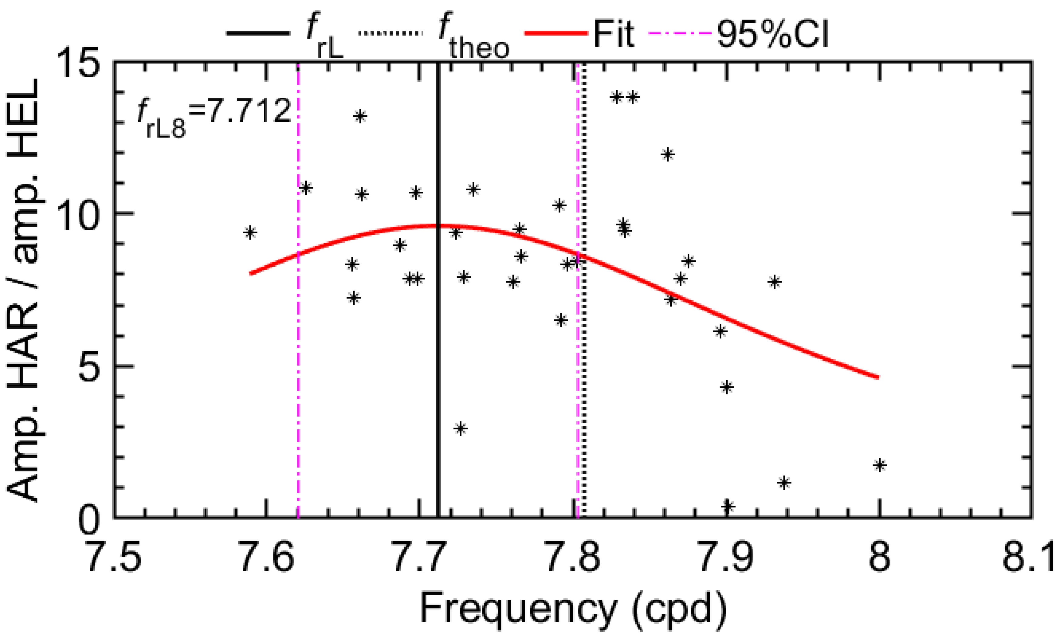
For further validation, the other resonance cases after Equation (5) for the system’s length to wavelength ratios 3/4 and 5/4 were calculated. The resonant frequency for the 3/4 case is 4.6845 cpd, which lies in a gap between the quarter- and fifth-diurnal tides. The 5/4 resonant frequency is 7.8074 cpd and thus located in the middle of the eighth-diurnal bandwidth (Figure 10). Here, an LCF delivers a resonance frequency of 7.712 cpd, 0.0954 cpd less than the theoretical resonance frequency. Conversely, this 5/4 resonance frequency calculated back indicates an 1/4 resonance frequency of 1.5424 cpd. This frequency is only 0.0191 cpd lower than the previously determined 1/4 resonance frequency and lies in its 95% confidence interval. As the amplitudes of the eighth diurnal tidal constituents are significantly smaller than the mean constituents in the diurnal and semidiurnal frequency domain, the dispersion of the amplification values is worse and the 95% confidence interval broad.
According to Equation (1), the resonance frequency depends on the length of the basin as well as its depth. Consequently, changing the estuary length or its depth alters the resonance frequency. Shortening and deepening the oscillatory estuary increases the resonance frequency, whereby shortening has the greater effect [23].
3.3.3. Node Migration
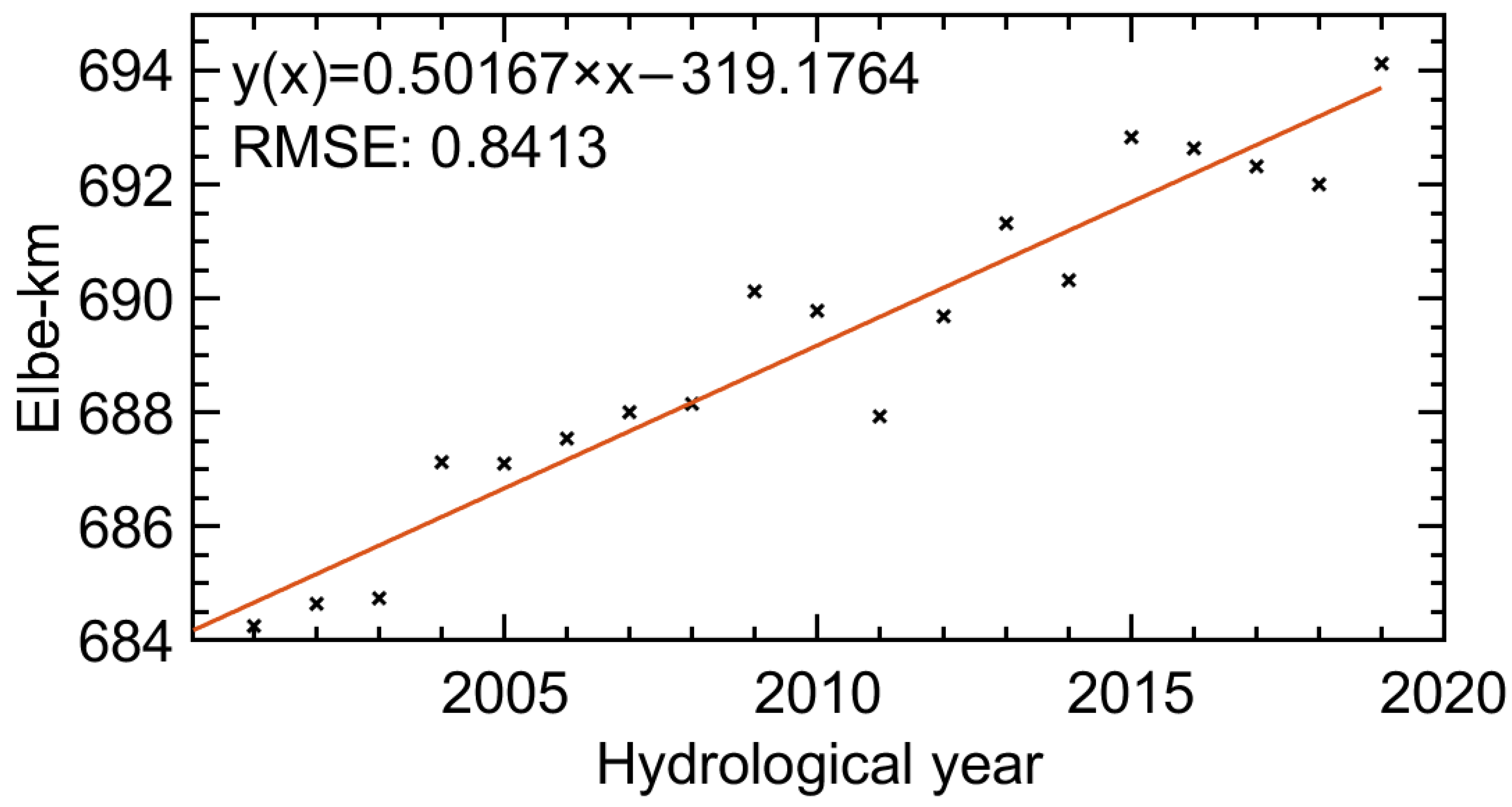
Node positions, determined as described in Section 2.4., indicate a linear trend of 0.5 km/a seaward migration (Figure 11). As stated by Proudman [1], full resonance occurs when the node is located at the open end of the estuary. Consequently, the seaward migration of the node could be interpreted as an increase in latent resonance. However, the spatial distribution of gauges downstream of Elbe-km 674 is with ca. 10 km to 12 km only half as good as in the upper part. Consequently, determinations of nodes in this area have major uncertainties and node positions differ by up to 3 km between adjacent years.
Potential reasons for seaward node migration are manifold but can be grouped to two main causes: a shortening of the estuary or a lengthening of the tidal wavelength. As no greater river engineering measures were conducted between 2000 and 2019, a shortening of the system is unlikely. Only a natural breach in the river mouth in 2008 might be interpreted as a shortening of the tidal wave’s ideal runway, but by no more than 2 km to 3 km.
A lengthening of the tidal waves is more reasonable. A reason for longer wavelengths can be greater water depths (Equation (1)). No waterway deepening was conducted between 2000 and 2019. However, sediment volume analyses show a loss from erosion, mainly between Elbe-km 660 and 685, indicate deepening of the mean riverbed between 2000 and 2010 [17]. Longer tidal waves can also be caused by a decrease of friction as stated in Equation (11) (from Parker [23], illustrated in his Figure 7), with wavelength L, wavenumber k and friction coefficient μ, where index 0 indicates the frictionless status:
Friction coefficients are unknown for the Elbe estuary, but there are hints that friction decreased over the investigation period. Weilbeer et al. [17] state that the previously mentioned erosion also decreased dune and ripple induced friction between Elbe-km 660 and 685. Additionally, they state that from 2010 to 2016 between Elbe-km 633 and 642, dune and ripple structures weakened significantly. Causes assumed by Weilbeer et al. [17] are increased sediment deposit due to the dredge spoil dumping at the river island Neßsand at river kilometre 633. Fine-grained sediments have been overlying dunes and ripples, partially leading to a complete absence, in particular since 2015, when sedimentation and dredging in the Port of Hamburg increased, due to extreme low river discharge [18]. Meanwhile in the outer Elbe estuary, the dune and ripple structures increased. Furthermore, fluid mud layers in the river branching area have been formed over the last years, which decreased friction [17]. Those decreases in friction have a self-regulation, because tidal wave amplitudes and current velocities increases with decreasing friction, which in turn increases quadratic-friction dissipation [37]. Another influencing factor, contributing to the seaward node migration is the decreasing river discharge. Since 2014, a period of distinctively decreased discharges is ongoing with a five-years mean (2015 to 2019) of 485 m3/s, leading to a drop in the 30-year running mean from 692 m3/s in 2000 to 649 m3/s in 2019. Backhaus [15] used river discharges between 0 m3/s and 3000 m3/s in steps of 300 m3/s in his one-dimensional numerical channel model and determined a seaward node migration of approximately 20 km between maximum and minimum discharge. However, such an increase in latent resonance might have added to the increase in tidal range from 3.63 m (5-year mean 2001–2005) to 3.82 m (5-year mean 2015–2019), but as the node position determination is vague, a longer investigation period with ideally additional gauges is needed to make well-founded statements.
4. Conclusions
The Elbe estuary with its large number of gauges distributed along the fairway has great potential for analysing the oscillatory behaviour of the tidal waves, providing an enhanced view into the tidal dynamics in estuaries and other tidal influenced basins. A total of 25 gauges with their high spatial resolution of an average distance of 7 km over a length of 170 km deliver digital data every minute continuously since 2000. This allows a detailed analysis of the tidal oscillation in an unprecedented resolution over the measurement duration covering an entire nodal cycle of 18.613 a. A self-programmed adapted harmonic analysis method of least squares (HAMELS) was used to determine the tidal wave spectra, providing advantages over conventional tools. Since the angular positions and nodal amplitude and phase modulations are directly considered in the multiple regression, calculated amplitudes and phases have a higher validity and principal tides and shallow water compound tides with the same mean frequency are distinguished. The determined tidal constituents allow the following conclusions about tidal wave transformation along the estuary:
- Semidiurnal tides lose dominance as the tidal wave progresses upstream, while higher harmonics and compound tides gain energy, causing the observable tidal asymmetry with shorter but stronger tides. Frequency group specific partial clapotis were determined significantly influencing the whole estuary and not just the landward 1/3 as stated by [11]. Together with the publications of Eichweber, Lange and Rolinski [12,13,14], both current velocity data and measured water levels now prove the existence of standing waves in the estuary.
- Significant differences in amplification of tidal constituents of similar frequencies were determined and their reasons discussed. It was demonstrated that shallow water compound tides with their nodal variations contribute to such differing degrees of amplification.
- The differences in amplification of energetic tidal constituents have direct influences on the superimposed tidal amplification and thus the tidal range inside the estuary. The significantly lower amplification of the S2 compared to the M2 is partly responsible for the fact that the degree of tidal amplification is negatively correlated with the incoming tidal range measured at Helgoland.
- Concerning tidal resonance in the estuary, a full established quarter-wavelength resonance in the Elbe estuary cannot be observed. It is shown that the nodal point of the tide is inside the estuary and not at its seaward end.
- A new test for tidal resonance via a three-parameter Lorentzian curve-fitting was developed and confirmed that full resonance is not established in the Elbe estuary. Instead, the natural resonance frequency of the Elbe estuary was calculated to 1.5615 cpd (period of 15.37 h). Nonetheless, the determined seaward node migration can be interpreted as an increasing latent resonance in the Elbe estuary. As no fairway deepening measures were conducted over the observation period, observed decreases in bottom friction and comparatively low river discharges are assumed as possible causes.
Based on this work, ongoing studies are going to determine the tidal oscillation’s temporal variation and dependencies on further influencing factors in the Elbe estuary.
Author Contributions
Conceptualization, S.S.V.H. and T.S.; methodology, S.S.V.H. and T.S.; software, S.S.V.H.; validation, S.S.V.H., V.S., E.N., T.S. and P.F.; formal analysis, S.S.V.H.; investigation, S.S.V.H. and T.S.; data curation, T.S.; writing—original draft preparation, S.S.V.H.; writing—review and editing, S.S.V.H., V.S., E.N., T.S. and P.F.; visualization, S.S.V.H.; supervision, E.N., T.S. and P.F.; project administration, E.N., T.S. and P.F.; funding acquisition, T.S. and P.F. All authors have read and agreed to the published version of the manuscript.
Funding
This research was funded by the German Federal Ministry of Education and Research, grant number 03KIS122.
Institutional Review Board Statement
Not applicable.
Informed Consent Statement
Not applicable.
Data Availability Statement
The water level data can be obtained via the website www.kuestendaten.de, accessed on 15 March 2021.
Acknowledgments
The studies presented in this publication are part of the German Coastal Engineering Research Council (KFKI) project RefTide. We acknowledge support for the Open Access fees by Hamburg University of Technology (TUHH) in the funding programme Open Access Publishing. The authors also would like to thank the Waterways and Shipping Offices Cuxhaven, Hamburg and Lauenburg for providing the water-level data.
Conflicts of Interest
The authors declare no conflict of interest. The funders had no role in the design of the study; in the collection, analyses, or interpretation of data; in the writing of the manuscript, or in the decision to publish the results.
References
- Proudman, J. Dynamical Oceanography; Methuen & Co.: London, UK, 1953. [Google Scholar]
- Marmer, H.A. Tides in the Bay of Fundy. Geogr. Rev. 1922, 12, 195–205. [Google Scholar] [CrossRef]
- Garrett, C. Tidal resonance in the Bay of Fundy and Gulf of Maine. Nature 1972, 238, 441. [Google Scholar] [CrossRef]
- Desplanque, C.; Mossman, D.J. Bay of Fundy tides. Geosci. Can. 2001, 28, 1–11. [Google Scholar]
- Bowen, A.; Gray, D. The tidal regime of the River Thames; long-term trends and their possible causes. Philos. Trans. R. Soc. London. Ser. A Math. Phys. Sci. 1972, 272, 187–199. [Google Scholar]
- Wang, Z.B.; Vandenbruwaene, W.; Taal, M.; Winterwerp, H. Amplification and deformation of tidal wave in the Upper Scheldt Estuary. Ocean Dyn. 2019, 69, 829–839. [Google Scholar] [CrossRef] [Green Version]
- Van Maren, D.; van Kessel, T.; Cronin, K.; Sittoni, L. The impact of channel deepening and dredging on estuarine sediment concentration. Cont. Shelf Res. 2015, 95, 1–14. [Google Scholar] [CrossRef] [Green Version]
- Boehlich, M.J.; Strotmann, T. The Elbe Estuary. Die Küste 2008, 74, 288–306. [Google Scholar]
- Aubrey, D.; Speer, P. A study of non-linear tidal propagation in shallow inlet/estuarine systems Part I: Observations. Estuar. Coast. Shelf Sci. 1985, 21, 185–205. [Google Scholar] [CrossRef]
- Speer, P.; Aubrey, D. A study of non-linear tidal propagation in shallow inlet/estuarine systems Part II: Theory. Estuar. Coast. Shelf Sci. 1985, 21, 207–224. [Google Scholar] [CrossRef]
- van Rijn, L.C. Analytical and numerical analysis of tides and salinities in estuaries; part I: Tidal wave propagation in convergent estuaries. Ocean Dyn. 2011, 61, 1719–1741. [Google Scholar] [CrossRef]
- Eichweber, G.; Lange, D. Über die Bedeutung der Reflexion von Obertiden für die Unterhaltungsaufwendungen in der Tideelbe. Die Küste 1996, 58, 179–198. [Google Scholar]
- Eichweber, G.; Lange, D. Tidal subharmonics and sediment dynamics in the Elbe Estuary. In Proceedings of the 3rd International Conference on Hydro-Science and -Engineering: Brandenburg University of Technology at Cottbus, Cottbus/Berlin, Germany, 31 August–3 September 1998. [Google Scholar]
- Rolinski, S.; Eichweber, G. Deformations of the tidal wave in the Elbe estuary and their effect on suspended particulate matter dynamics. Phys. Chem. Earth Part B Hydrol. Ocean. Atmos. 2000, 25, 355–358. [Google Scholar] [CrossRef]
- Backhaus, J.O. Latent resonance in tidal rivers, with applications to River Elbe. J. Mar. Syst. 2015, 151, 71–78. [Google Scholar] [CrossRef]
- Hartwig, F. Das Schwingungsverhalten der Tideelbe hinsichtlich Resonanz. Die Küste 2016, 84, 193–212. [Google Scholar]
- Weilbeer, H.; Winterscheid, A.; Strotmann, T.; Entelmann, I.; Shaikh, S.; Vaessen, B. Analyse der Hydrologischen und Morphologischen Entwicklungen in der Tideelbe für den Zeitraum 2013–2018. Die Küste. Under review.
- Boehlich, M.J.; Strotmann, T. Das Elbeästuar. Die Küste 2019, 87. [Google Scholar] [CrossRef]
- Boehlich, M.J. Tidedynamik der Elbe. Mitt. Bundesanst. Wasserbau 2003, 86, 55–60. [Google Scholar]
- Schureman, P. Manual of Harmonic Analysis and Prediction of Tides; US Department of Commerce: Washington, DC, USA, 1958; Volume Special Publication No. 98. [Google Scholar]
- Doodson, A.T. The harmonic development of the tide-generating potential. Proc. R. Soc. Lond. Ser. A Contain. Pap. A Math. Phys. Character 1921, 100, 305–329. [Google Scholar]
- International Astronomical Union Standards of Fundamental Astronomy. Available online: http://www.iausofa.org (accessed on 13 June 2019).
- Parker, B.B. Tidal Analysis and Prediction; US Department of Commerce: Silver Spring, MD, USA, 2007; Volume NOAA Special Publication NOS CO-OPS 3. [Google Scholar]
- IHO—International Hydrographic Organization. Harmonic Constants Product Specification; Version 1.0; Tides Committee of the International Hydrographic Organization: Monaco, 2006. [Google Scholar]
- Boon, J.D., III; Kiley, K.P. Harmonic Analysis and Tidal Prediction by the Method of Least Squares: A User’s Manual. Special Reports in Applied Marine Science and Ocean Engineering (SRAMSOE): Virginia Institute of Marine Science, College of William and Mary; W & M ScholarWorks: Williamsburg, VA, USA, 1978; No. 186. [Google Scholar]
- Codiga, D.L. Unified Tidal Analysis and Prediction Using the UTide Matlab Functions; Graduate School of Oceanography, University of Rhode Island Narragansett: Kingston, RI, USA, 2011. [Google Scholar]
- Roos, A. Tides and Tidal Currents. Lect. Note IHE Delft. 1997. Available online: http://resolver.tudelft.nl/uuid:95d4e53a-8e9f-4550-a601-b50a0de2498f (accessed on 19 December 2018).
- Mikhailov, E.E. Fitting and data reduction. In Programming with MATLAB for Scientists: A Beginner’s Introduction; CRC Press: Boca Raton, FL, USA, 2018. [Google Scholar]
- Robinson, M.; Clegg, J. Improved determination of Q-factor and resonant frequency by a quadratic curve-fitting method. IEEE Trans. Electromagn. Compat. 2005, 47, 399–402. [Google Scholar] [CrossRef]
- Betzler, K. Fitting in Matlab. Fachbereich Phys. Univ. Osnabr. 2003. Available online: https://www.betzler.physik.uni-osnabrueck.de/Manuskripte/short/fits.pdf (accessed on 17 March 2021).
- Gönnert, G.; Isert, K.; Giese, H.; Plüß, A. Charakterisierung der Tidekurve. Die Küste 2004, 68, 99–141. [Google Scholar]
- Redfield, A.C. The Analysis of Tidal Phenomena in Narrow Embayments; Massachusetts Institute of Technology and Woods Hole Oceanographic Institution: Woods Hole, MA, USA, 1950. [Google Scholar]
- Parker, B.B. Frictional effects on the tidal dynamics of a shallow estuary. Ph.D. Thesis, The Johns Hopkins University, Baltimore, Maryland, 1984. [Google Scholar]
- Hunt, J. Tidal oscillations in estuaries. Geophys. J. Int. 1964, 8, 440–455. [Google Scholar] [CrossRef] [Green Version]
- Backhaus, J.O. Improved representation of topographic effects by a vertical adaptive grid in vector-ocean-model (VOM). Part I: Generation of adaptive grids. Ocean Model. 2008, 22, 114–127. [Google Scholar] [CrossRef]
- Backhaus, J.O.; Harms, I.; Hübner, U. Improved representation of topographic effects by a vertical adaptive grid in Vector-Ocean-Model (VOM). Part II: Simulations in unstructured adaptive grids. Ocean Model. 2008, 22, 128–145. [Google Scholar] [CrossRef]
- Dietrich, G.; Kalle, K.; Krauss, W.; Siedler, G. Gezeitenerscheinungen. In Allgemeine Meereskunde: Eine Einführung in Die Ozeanographie; Gebr. Borntraeger: Berlin, Germany, 1975. [Google Scholar]
Figure 1.
Overview of the Elbe estuary. Bathymetry data after the digital terrain model water DGMW-2016.
Figure 1.
Overview of the Elbe estuary. Bathymetry data after the digital terrain model water DGMW-2016.

Figure 2.
Fairway bathymetry averaged over 1 km representative for the investigation period, and mean sea level (MSL) for river discharges of 350 m3/s and 1500 m3/s.
Figure 2.
Fairway bathymetry averaged over 1 km representative for the investigation period, and mean sea level (MSL) for river discharges of 350 m3/s and 1500 m3/s.

Figure 3.
Typical forms of diurnal, semidiurnal, quarter-diurnal and sixth-diurnal tides in the Elbe estuary normalised to incoming amplitudes measured at beacon A. Separated datum points show gauge Helgoland in the German Bight. Harmonic analysis method of least squares (HAMELS) conducted without compound tides over a nodal cycle beginning at 1 January 2000 12:00:00 considering nodal corrections.

Figure 4.
Amplitude on the S2 frequency, determined for 365.25 d intervals, shifted by 29.5 d shown together with a share of the node factor f of the K1 (f(K1) = f(KP2)).
Figure 4.
Amplitude on the S2 frequency, determined for 365.25 d intervals, shifted by 29.5 d shown together with a share of the node factor f of the K1 (f(K1) = f(KP2)).

Figure 5.
Phase on the S2 frequency, determined for 365.25 d intervals, shifted by 29.5 d shown together with the nodal phase correction u of the K1 (u(K1) = u(KP2)).
Figure 5.
Phase on the S2 frequency, determined for 365.25 d intervals, shifted by 29.5 d shown together with the nodal phase correction u of the K1 (u(K1) = u(KP2)).

Figure 6.
Tidal constituents S2 and the shallow water compound tide KP2 considering its nodal amplitude and phase correction. The fitting curve includes amplitudes of M2, S2 and N2 without consideration of compound tides.
Figure 6.
Tidal constituents S2 and the shallow water compound tide KP2 considering its nodal amplitude and phase correction. The fitting curve includes amplitudes of M2, S2 and N2 without consideration of compound tides.

Figure 7.
Tidal constituents S2 and the shallow water compound tide KP2 considering only its nodal amplitude correction f without the phase correction. The fitting curve includes amplitudes of M2, S2 and N2 without consideration of compound tides.
Figure 7.
Tidal constituents S2 and the shallow water compound tide KP2 considering only its nodal amplitude correction f without the phase correction. The fitting curve includes amplitudes of M2, S2 and N2 without consideration of compound tides.

Figure 8.
Relationship between the ratio of tidal range in the port of Hamburg at St. Pauli (STP) and the offshore gauge at Helgoland island (HEL) in the German Bight plotted against the tidal range of the respective tide at Helgoland for the hydrological years 2000 to 2019.
Figure 8.
Relationship between the ratio of tidal range in the port of Hamburg at St. Pauli (STP) and the offshore gauge at Helgoland island (HEL) in the German Bight plotted against the tidal range of the respective tide at Helgoland for the hydrological years 2000 to 2019.

Figure 9.
Degrees of amplification between gauge Helgoland in the German Bight and gauge Harburg at the reflector in the Southern Elbe, where maximal tidal ranges are measured, for diurnal and semidiurnal tidal constituents. Additionally shown are the resonance frequency of the Elbe estuary calculated via a three-parameter Lorentzian function-fit frL and after Backhaus [15] frB.

Figure 10.
Degrees of amplification between gauge Helgoland in the German Bight and gauge Harburg at the reflector in the port of Hamburg for eighth-diurnal tidal constituents. Additionally shown are the resonance frequency calculated via a three-parameter Lorentzian function-fit frL and the theoretical frequency ftheo for the system length to wavelength ratio of 5/4 (5 × 1.5615 cpd).

Figure 11.
Positions of the partial clapotis’ node over the hydrological years 2000 to 2019 and linear regression line.
Figure 11.
Positions of the partial clapotis’ node over the hydrological years 2000 to 2019 and linear regression line.


Table 1.
Solar and lunar elements with their average period and composition from orbital parameters.
Table 1.
Solar and lunar elements with their average period and composition from orbital parameters.
| Lunar/Solar Element | Mean Period | Composition |
|---|---|---|
| s | 27.32158226 d | F + N |
| h | 365.2421891 d | FD + N |
| p’ | 8.847310062 a | F − M’ + N |
| N | 18.61281593 a | Ω |
| p | 20942 a | F − D + N − M |
Table 2.
M2 and S2 amplitudes as well as spring and neap tidal range resulting from M2 and S2 interference for gauges Helgoland (HEL), beacon A (BKA) and St. Pauli (STP) as well as amplification ratios between STP and the other two gauges.
Table 2.
M2 and S2 amplitudes as well as spring and neap tidal range resulting from M2 and S2 interference for gauges Helgoland (HEL), beacon A (BKA) and St. Pauli (STP) as well as amplification ratios between STP and the other two gauges.
| Composition | HEL (cm) | BKA (cm) | STP (cm) | STP/HEL | STP/BKA |
|---|---|---|---|---|---|
| Amp. M2 | 110 | 137 | 160 | 1.45 | 1.17 |
| Amp. S2 | 29 | 36 | 37 | 1.28 | 1.03 |
| Neap: 2 × (M2 − S2) | 162 | 246 | 246 | 1.52 | 1.22 |
| Spring: 2 × (M2 + S2) | 278 | 394 | 394 | 1.42 | 1.14 |
Publisher’s Note: MDPI stays neutral with regard to jurisdictional claims in published maps and institutional affiliations. |
© 2021 by the authors. Licensee MDPI, Basel, Switzerland. This article is an open access article distributed under the terms and conditions of the Creative Commons Attribution (CC BY) license (http://creativecommons.org/licenses/by/4.0/).
Share and Cite
MDPI and ACS Style
Hein, S.S.V.; Sohrt, V.; Nehlsen, E.; Strotmann, T.; Fröhle, P. Tidal Oscillation and Resonance in Semi-Closed Estuaries—Empirical Analyses from the Elbe Estuary, North Sea. Water 2021, 13, 848. https://doi.org/10.3390/w13060848
AMA Style
Hein SSV, Sohrt V, Nehlsen E, Strotmann T, Fröhle P. Tidal Oscillation and Resonance in Semi-Closed Estuaries—Empirical Analyses from the Elbe Estuary, North Sea. Water. 2021; 13(6):848. https://doi.org/10.3390/w13060848
Chicago/Turabian StyleHein, Sebastian S. V., Vanessa Sohrt, Edgar Nehlsen, Thomas Strotmann, and Peter Fröhle. 2021. "Tidal Oscillation and Resonance in Semi-Closed Estuaries—Empirical Analyses from the Elbe Estuary, North Sea" Water 13, no. 6: 848. https://doi.org/10.3390/w13060848
Note that from the first issue of 2016, this journal uses article numbers instead of page numbers. See further details here.