Modelling of Pool-Type Fishways Flows: Efficiency and Scale Effects Assessment

Abstract

In this study, the 3D numerical modelling of flow in a pool-type fishway with bottom orifices was performed using computational fluid dynamics (CFD) software (FLOW-3D^®). Numerical results were compared with experimental data obtained from acoustic Doppler velocimetry (ADV) and particle image velocimetry (PIV) measurements. Several hydrodynamic variables that influence fishways efficiencies, such as flow depths, flow patterns, water velocity, turbulent kinetic energy, Reynolds normal stresses, and Reynolds shear stress parallel to the bottom component, were qualitatively and quantitatively compared. The numerical model accurately reproduced the complex flow field, showing an overall good agreement between the numerical model predictions and the experimental data for the analysed variables. The importance of performing a numerical model validation for all the parameters under analyses was highlighted. Additionally, scaling effects were analysed by running an upscaled numerical model of the prototype fishway. The model performed with similar accuracy for both physical model and prototype dimensions with no evidence of scale effects. The present study concludes that CFD models (namely FLOW-3D^®) may be used as an adequate and efficient design and analysis tool for new pool-type fishways geometries, reducing and complementing physical model testing.

1. Introduction

Restoring the longitudinal connectivity of rivers remains a key issue in the recovery of freshwater ecosystems [1,2]. If well designed and constructed, fishways provide a path that allows fish to continue migrating past dams and weirs. In a review of fish passage efficiency, Noonan et al. [3] found that the design features of many existing fishways did not meet the needs of fish species adequately, although pool-type fishways presented the highest efficiency for all fish groups.

Providing suitable swimming conditions for multiple fish species is rather challenging since the flow and turbulence patterns in fishways play a major role in their success [2,4,5,6,7,8,9,10,11,12]. Physical modelling has been the main approach to study the hydrodynamics of pool-type fishways (e.g., [13,14,15,16,17,18,19,20,21,22]). However, physical experiments are expensive and time-consuming. Therefore, with the advances in computer technology, computational fluid dynamics (CFD) three-dimensional (3D) models are increasingly being used to analyse the flow patterns in hydraulic structures with complex geometry, in order to reduce physical model testing [23,24]. Thus, these models may play an essential role in the study of fishway hydrodynamics and the design of efficient fishways.

Numerical modelling studies on fishways have been mainly focused on vertical slot fishways [12,25,26,27,28,29,30,31,32,33,34,35,36,37]. Since vertical slot fishways flow in the major part of a pool is almost two-dimensional (2D), with vertical velocity components much smaller than the horizontal ones [26], most of these studies used 2D models.

In pool-type fishways with bottom orifices, the flow is highly complex and 3D, requiring the use of 3D models to obtain an accurate flow field characterization. Modelling this fishway configuration is rather challenging since it involves high velocity gradients, high vorticity, and high shear regions. In this study, 3D numerical simulations of a pool-type fishway with bottom orifices were performed using FLOW 3D^® (Flow Science, Inc., Santa Fe, NM, USA) to assess its ability to predict flow depth, velocity, and turbulence patterns.

In recent years, an indoor near-prototype pool-type fishway was used to study cyprinid species behaviour and movements [1,7,8,11,38,39,40,41,42,43]. Silva et al. [38] assessed the response of the Iberian barbel Luciobarbus bocagei (Steindachner, 1864) to the simultaneous presence of submerged orifices and surface notches with adjustable dimensions in association with two different flow regimes over the notches, plunging, and streaming. The results of this study showed that Iberian barbel preferred the orifices (76%) to negotiate the fishway and that the time taken to enter the fishway was also much smaller for the orifices. Silva et al. [39] tested the suitability for Iberian barbel of a pool-type fishway with offset and straight orifices. This study found that the offset configuration had a significantly higher rate of fish passage success (68%), comparatively to the straight orifice layout (28%). The time taken to successfully negotiate the fishway was also significantly lower for the offset configuration, particularly for small adults. The effects of water velocity and turbulence parameters on fish swimming performance was analysed in this study. To characterize the flow fields in a pool, an acoustic Doppler velocimeter was used. According to the findings of this study Reynolds shear stress proved to be the parameter that most strongly influenced the movements of Iberian barbel within the fishway. Branco et al. [40] assessed the behaviour and performance of two species with different morphological and ecological characteristics, the bottom oriented Iberian barbel Luciobarbus bocagei, and the water column swimmer Iberian chub Squalius pyrenaicus, in a pool-type fishway with orifices and notches with two different flow regimes, plunging and streaming. To characterize the hydrodynamics of a pool, an acoustic Doppler velocimeter was used. Results showed that both species preferred the notch with streaming flow and were more successful in moving upstream with this flow regime.

In this study, a 1:2.5 scaled fishway model of this facility was used to measure the velocity and turbulence in a pool-type fishway with bottom orifices configuration tested by Silva et al. [7,38] using barbels that proved to be effective. Extensive measurements of instantaneous velocities with a 2D particle image velocimetry (PIV) system and acoustic Doppler velocimetry (ADV) were performed, postprocessed, and used to assess the numerical model accuracy. Haque et al. [44] referred to the problems that, in most cases, the experimental data sets, available for numerical models’ validation, have high measurement errors, and/or the measurement meshes are too coarse to be able to correctly assess the predictive capabilities of these models. Blocken and Gualtieri [23] mention that verification and validation studies are indispensable and high-quality experiments are needed to supply data to validate CFD studies. Fuentes-Pérez et al. [35] also refer to the difficulty in finding numerical model validation data in fishway studies, especially for turbulence metrics. Due to the use of two measurement techniques and to the significant amount of experimental data obtained, these problems were overcome in this study.

Physical models are frequently based on the Froude number similarity, being the Reynolds number similarity ignored due to difficulties in meeting both similarity laws. Since the prototype Reynolds number is normally much larger, Reynolds number-related scale effects might be introduced. The Reynolds number increase may affect the velocity distribution and the boundary layer properties [45]. Numerical simulations may be used to assess the scale effects [46,47]. Thus, in this study, to analyse the scale effects on pool-type fishways with bottom orifices flow, two different sized numerical models were developed: a large-sized model with the prototype dimensions and a scaled small-sized one with the physical model dimensions.

The flow field in pool-type fishways with bottom orifices is highly three-dimensional and much more complex than the flow field in vertical slot fishways (VSF), which is the design more frequently considered in previous studies on fishways numerical model validation [26,27,28,29,35]. To the authors’ best knowledge, this is the first CFD study on pool-type fishways with bottom orifices, which also includes the most extensive comparison between experimental velocity data and three-dimensional numerical modelling results on pool-type fishways published. Two different measurement techniques (PIV and ADV), were used, thus allowing a detailed comparison and providing confidence in the results on CFD simulations for this type of flow field.

The study presents not only a qualitative comparison but also a detailed quantitative comparison, with statistical testing on the agreement between the numerical model results and measurements, including turbulence parameters, which was not presented in previous numerical model studies of other fishway types. Scale effects are addressed as well. Hence, this study will smooth the validation of CFD models of pool-type fishways, the most used worldwide [10], and it will hopefully encourage its use by the designers.

Furthermore, the use of CFD models (namely FLOW 3D^®) as a design tool for new pool-type fishways geometries is discussed.

2. Materials and Methods

2.1. Experimental Setup and Procedure

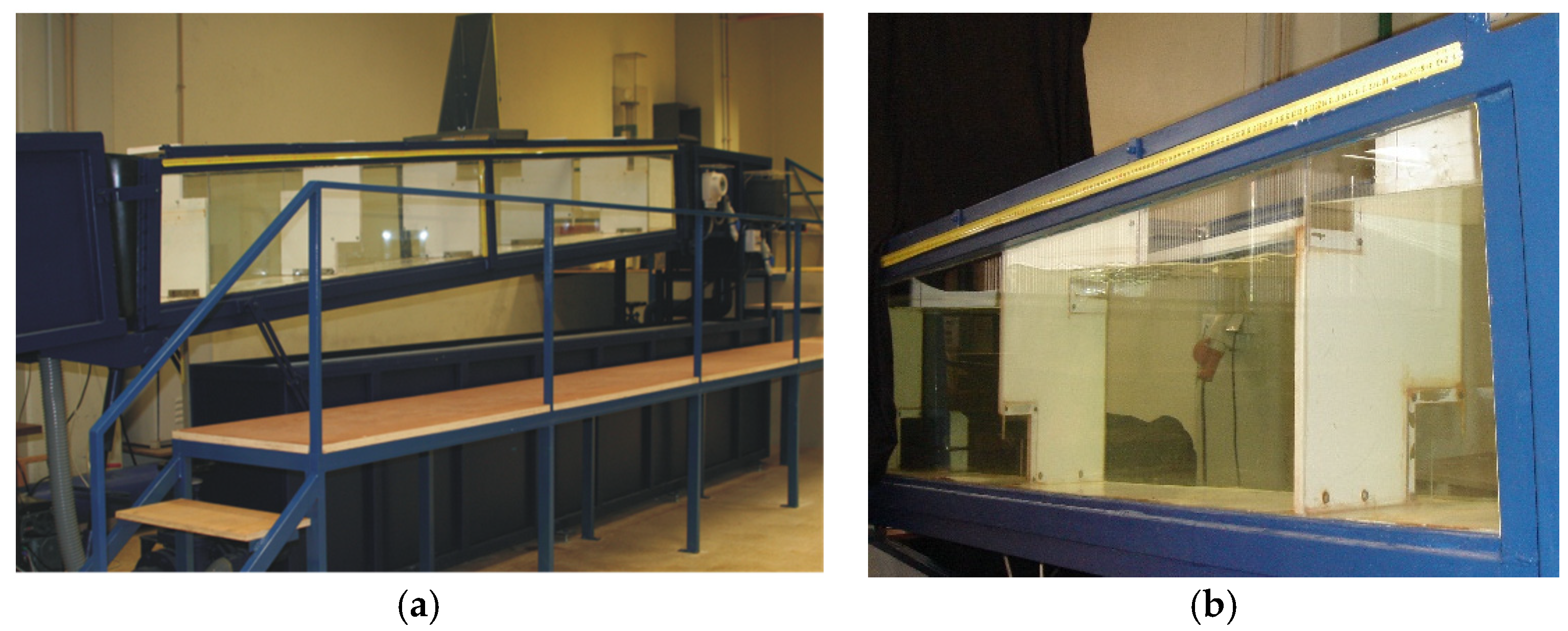
The facility where the experimental work was undertaken is located at the Laboratory of Hydraulics and Environment of Instituto Superior Técnico (IST, Lisboa, Portugal). It is a 1:2.5 scaled fishway of a prototype size indoor pool-type fishway located at the National Laboratory for Civil Engineering (LNEC, Lisboa, Portugal). It includes a 5.7 m long, 0.4 m wide, and 0.5 m deep flume, with an adjustable slope, equipped with a recirculation circuit and a pump frequency converter. An electromagnetic flow meter, installed in the recirculation circuit, measures the discharge that is controlled by the pump frequency converter. A sluice valve controls the downstream flow depth. The flume has glass side walls, enabling flow visualization and PIV measurements (Figure 1).

Five PVC cross-walls equipped with bottom orifices of 0.08 × 0.08 m² were used to create four fishway pools, each 0.76 m long, 0.40 m wide, and 0.50 m deep. The orifices were created using a thin (2 mm) perspex plate, and the edges were sharp-crested. Consecutive orifices were positioned on opposite sides of the cross-walls (Figure 1b), creating a sinusoidal flow path.

The flume was set at a slope of 8.5%, which is within the range of slopes commonly used in prototype fishways [48] and used in previous experiments with fish in the near-prototype fishway previously mentioned [7]. The discharge was set to 4.4 ± 0.4% Ls⁻¹, the head drop between pools (Δh) was 0.064 ± 5% m, and the pool mean water depth (h_m) was 0.352 ± 0.5% m. These values were scaled from the experiments performed by Silva et al. [7] and were controlled and maintained constant during all the experiments.

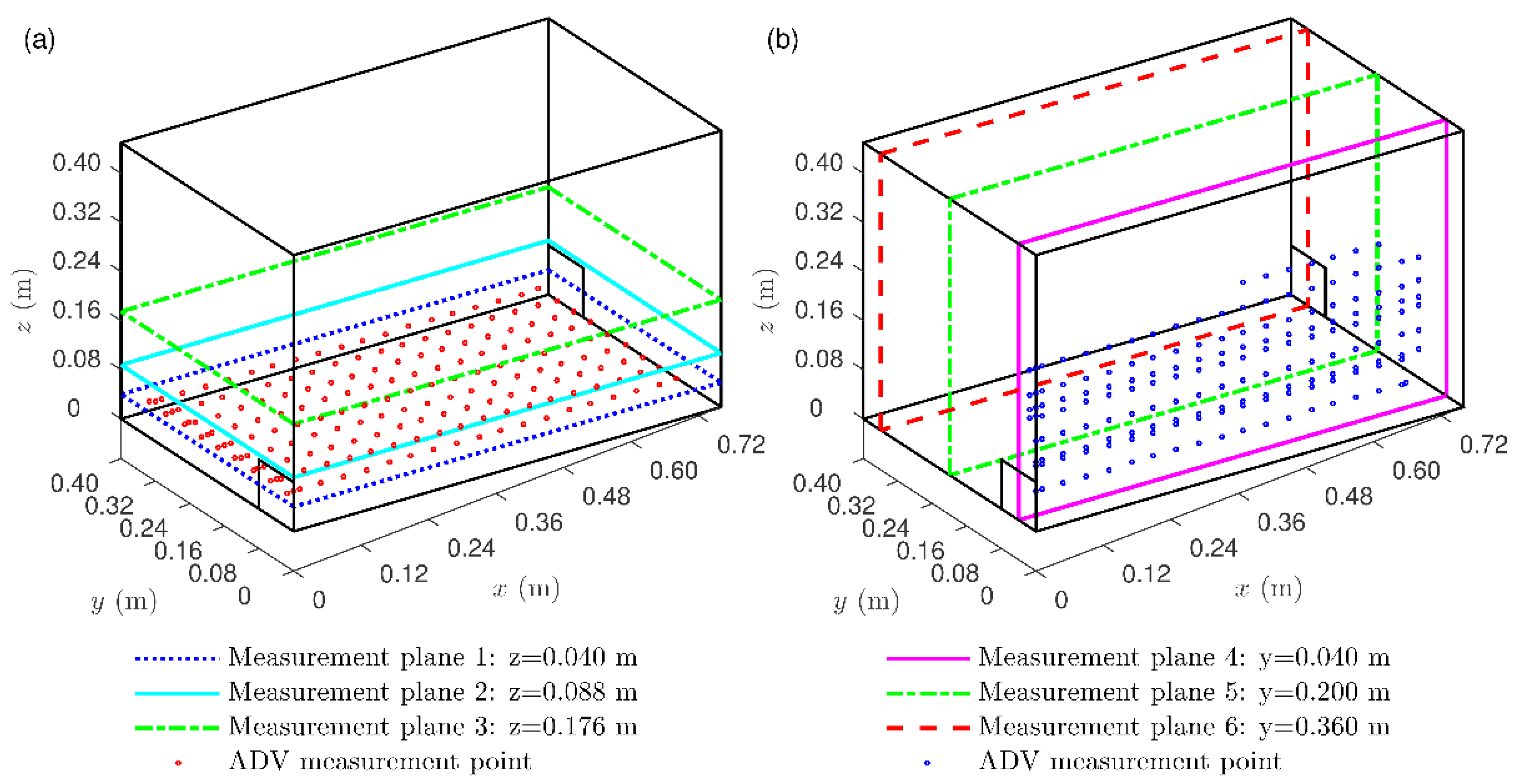
The PIV and ADV measurements were carried out in the third pool in six planes: three planes parallel to the flume bottom at 11.4% h_m (0.04 m—half the height of the orifice), 25% h_m, and 50% h_m, and three vertical planes parallel to the sidewalls at the mid-width of the pool and of each orifice (Figure 2). The planes of the instantaneous velocities’ measurement were chosen to provide an adequate characterization of the flow field in the range 0–50% h_m, which according to Silva et al. [7] is the region where fish were mostly found. In Quaresma et al. [49] a complete outline of the PIV and ADV measurements can be found.

The coordinate system has its origin in the bottom right corner of the third pool upstream orifice, with the longitudinal x-axis parallel to the bottom and the flume axis, the y-axis transversal and with the z-axis perpendicular to the bottom. The instantaneous velocity components u, v, and w correspond to the x-, y-, and z-axis, respectively.

2.2. Numerical Model

The numerical simulations were performed using FLOW-3D^®. This software is a general-purpose CFD program based on the finite volumes method that solve the equations of motion for fluids to obtain transient, three-dimensional solutions to multiscale and multiphysics flow problems [50]. In FLOW-3D^®, the computational domain is subdivided using Cartesian coordinates into a structured mesh grid of variable-sized hexahedral cells. The grid is defined independently of the geometry and, subsequently, the geometry is embedded in the grid by the Fraction Area/Volume Obstacle Representation (FAVOR^TM) technique [51]. Flow Science [50] presents additional details regarding the theoretical and numerical fundamentals of FLOW-3D^®. FLOW-3D^® has been used to model flows in fishways, hydraulic structures, and river reaches and bends (e.g., [45,52,53,54,55,56]).

In this study, the simulations were performed using the implicit solver generalized minimum residual method, which is highly accurate and efficient for a wide range of problems [50]. Several options of the software were investigated, namely the choice of the volume-of-fluid method, momentum advection method, turbulence model, and the roughness effect. To track the free surface, the VOF^TM (volume-of-fluid) method [57] was used. The selected momentum advection method was the second-order monotonicity preserving method, which is based on a second-order, monotonicity-preserving upwind-difference method [58]. All the turbulence models available in FLOW-3D^®, namely, the Re-Normalization Group (RNG), k-ε, k-ω turbulence models and Large-Eddy Simulation (LES) model were investigated. The results presented in this paper were obtained with the LES model, which presented the best agreement with the experimental results.

The roughness effect was also investigated by testing a range of Manning’s surface roughness coefficients that cover the experimental model materials possible values. The wall roughness was set using the roughness height computed from the Strickler formula. The Manning’s surface roughness that led to the best agreement between simulated and measured discharges and flow depths was n = 0.01 sm^−1/3. The acceleration of gravity was applied in the negative z-direction and in the positive x-direction so that the x-axis was parallel to the flume bottom. The upstream and downstream boundaries were specified as pressure boundary conditions based on the water depths observed experimentally (0.33 m and 0.40 m, respectively). At the side and bottom no-slip wall boundaries were used and at the top, a symmetry boundary condition (zero value for normal velocity, zero gradients for the other quantities) was specified. In free surface simulations, FLOW-3D^® neglects the inertia of the gas adjacent to the liquid, and the volume occupied by the gas is replaced with an empty space, void of mass, represented only by uniform pressure and temperature. Therefore, free surface becomes one of the flow external boundaries. With this approach the computational effort is reduced, since the details of the gas motion are not important for the motion of the much denser liquid. To accurately capture the free-surface dynamics, the VOF^TM method is employed. This method consists of three main components: (i) the definition of the volume of fluid function, (ii) a method to solve the VOF transport equation, and (iii) setting the boundary conditions at the free surface. The simulations were run for a number of time steps enough to attain a statistically stationary solution and obtain converged time-averaged values.

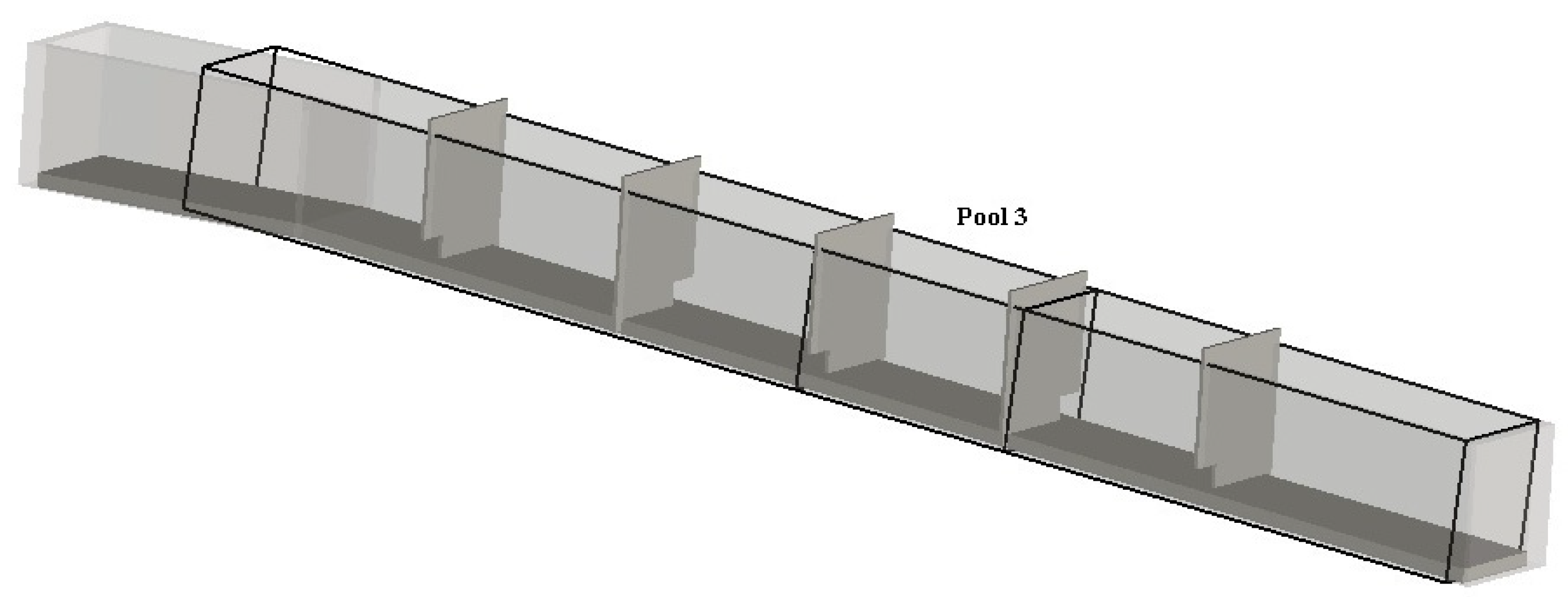
The fishway geometry was generated using AutoCAD 2014 (AutoDesk, San Rafael, CA, USA) based on the dimensions of the physical model and was imported into the code as a stereolithography (stl) file. The computational domain (Figure 3) was discretized using a multiblock grid. The grid was constituted of five blocks; one contained the entire geometry with a uniform grid spacing of 0.02 m. The other four blocks were nested blocks with a uniform grid spacing of 0.01 m; one contained the third pool, and the other three blocks contained the remaining cross-walls. This cell size is in line with previous works, e.g., Fuentes-Pérez et al. [35] for a vertical slot fishway with a slot width of 0.281 m used a cell size of 0.03 m, approximately 10.7% of the slot width (in the present study, a cell size of 0.01 m represents 12.5% of the orifice width). A total of 380,650 grid cells were used to represent the fishway geometry in the coarser mesh hereafter, named mesh A_model.

Since the choice of the mesh element size is highly case-specific [55], to test the influence of the grid resolution on the results, a mesh sensitivity analysis was performed, based on the ASME criteria [55,59] with three more grids. One, with 2,714,000 grid cells, was obtained by considering a grid spacing of 0.01 m in the block that contained the entire geometry and a grid spacing of 0.005 m in the block that contained the third pool. This mesh is named mesh B_model in this paper. Two more grids were considered using the grid overlay boundary condition available in FLOW-3D^® on the third pool mesh block. These grids had uniform grid spacings of 0.0025 m and 0.0020 m for mesh C_model and D_model, respectively.

To analyse the scale effects, a numerical model of a prototype size pool-type fishway (LNEC’s flume) was used. This model (the prototype model) was geometrically similar to the IST flume model and the scale ratio of length was 2.5. Two grids were used, A_prototype and B_prototype. The computational meshes of the prototype and the physical model were also adjusted according to the geometric similarity to exclude the generation of numerical errors due to different scaled meshes.

Table 1. Characteristics of the numerical meshes.

Mesh	Number of Mesh Blocks	Cell Sizes (Δx × Δy × Δz) (cm3)	Number of Cells	Computation Time for 10 s of Simulation Time (h) (a)
Amodel	5	2 × 2 × 2 1 × 1 × 1	380,650	2.1
Bmodel	2	1 × 1 × 1 0.5 × 0.5 × 0.5	2,714,000	11.2
Cmodel	1	0.25 × 0.25 × 0.25	12,364,800	98.7
Dmodel	1	0.20 × 0.20 × 0.20	23,417,910	268.8
Aprototype	5	5 × 5 × 5 2.5 × 2.5 × 2.5	380,650	0.5
Bprototype	2	2.5 × 2.5 × 2.5 1.25 × 1.25 × 1.25	2,714,000	8.7

^(a) with an Intel(R) Core(TM) i7-3770 [email protected] GHz (Intel Corporation, Santa Clara, CA, USA), 32.0 GB RAM, AMD Radeon HD 6450 (AMD Inc., Santa Clara, CA, USA). Δx—cell size in the x-direction; Δy—cell size in the y-direction; Δz—cell size in the z-direction.

presents the characteristics of the numerical meshes used in the present study and the computation time per 10 s of simulation time for each of the meshes.

2.3. Grid Resolution and Quality Verification

LES models use a spatial filter to separate the turbulent flow field into two components: the larger and more energetic turbulent structures that are resolved by the numerical method on a given mesh (resolved scales); and the smaller structures that are not captured by the mesh (sub-grid scales). The influence of subgrid scales on resolved scales must be modelled [24]. In FLOW-3D^®, the subgrid scales’ effects of turbulence are represented by an eddy viscosity, which is proportional to a length scale times a measure of velocity fluctuations on that scale. FLOW-3D^® uses the Smagorinsky method [60] which considers for the length scale the geometric mean of the grid cell dimensions (L = (Δx Δy Δz)^1/3). When using LES and implicit filtering, as the Smagorinsky method, since the filter size changes with the grid size and both the numerical discretization error and the sub-grid scale contributions are proportional to grid size, there is no grid-independent LES [61,62,63,64]. Considering this, Celik et al. [63] proposed the LES_IQ index to assess the quality of LES models. The LES_IQ_k index is a measure of the percentage of the resolved turbulent kinetic energy (TKE) to the total. This index gives an indication of the resolution quality in LES models.

To apply the LES_IQ index it must be checked if the grids are in the asymptotic range. Therefore, the observed apparent order of the method p for the hydraulic parameters under analysis in this study was computed following the procedure outlined in Celik et al. [60].

Table 2. Average apparent order of the method, p, and percentage of points showing oscillatory convergence.

Parameter	p	Percentage of Points Showing Oscillatory Convergence
$\overline{\mathbf{u}}$	1.9	27
$\overline{\mathbf{v}}$	1.7	56
$\overline{\mathbf{w}}$	2.1	58
$\overline{\mathbf{U}}$	1.9	61
$\overline{{{\mathrm{u}}^{\prime }}^2}$	1.8	59
$\overline{{{\mathrm{v}}^{\prime }}^2}$	1.6	64
$\overline{{{\mathrm{w}}^{\prime }}^2}$	1.6	65
κ	1.6	66
τuv	1.5	56

$\overline{\mathrm{u}}$, $\overline{\mathrm{v}}$, $\overline{\mathrm{w}}$ are the mean longitudinal, transversal, and vertical velocity component;$\overline{\mathrm{U}}$ is the mean velocity magnitude; $\overline{{{\mathrm{u}}^{\prime }}^2},\overline{{{\mathrm{v}}^{\prime }}^2},\overline{{{\mathrm{w}}^{\prime }}^2}$ = longitudinal, transversal, and vertical Reynolds normal stress; k is the turbulent kinetic energy; τ_uv is the parallel to the bottom Reynolds shear stress component.

shows the average apparent order of the method, p, and the percentage of points showing oscillatory convergence for the ADV measurement grid points locations.

The average observed apparent order of the method for all parameter under analysis is close to 2, which shows a good agreement with the formal order of the scheme used and indicates that the grids are within the asymptotic range [59]. The high percentage of points showing oscillatory convergence might be due to the fact that this flow field presents several recirculation regions [49]. Celik et al. [65] showed that the oscillatory convergence behaviour in finite difference solutions may be caused by the oscillatory velocity field that occurs in recirculation regions. This topic will be further addressed in the Appendix A.

Given the high number of points showing oscillatory behaviour, the modified version of LES_IQ_k index [62] was used to assess the resolution quality of the grids used and was computed in all ADV measurement grid points locations. Mesh A_model has an average LES_IQ_k index of 0.72 with 45% of the points with values higher than 0.80. When using the theoretical order of the scheme (p = 2) instead of the observed apparent order of the method Mesh A_model, the average LES_IQ_k index increases to 0.75, with 49% of the points with values higher than 0.8. The average LES_IQ_k index of the Mesh B_model is 0.90, with 89% of the points presenting values higher than 0.80. When using the theoretical order of the scheme (p = 2), instead of the observed apparent order of the method Mesh B_model, the average LES_IQ_k index increases to 0.93, with 98% of the points with values higher than 0.80.

According to Pope [66], a good LES should resolve at least 80% of the TKE. Celik et al. [62] consider that a LES_IQ_k of 75 to 85% can already be considered adequate for most engineering applications that typically occur at high Reynolds numbers. This flow field is highly complex and turbulent with a rapid mixing. Considering the mean velocity in the pool and the pool mean water depth, the Reynolds number is higher than 5 × 10⁵; thus, a LES_IQ_k of 75 to 85% can already be considered adequate. The values obtained for Mesh A_model and B_model indicate that sufficient grid resolutions were used. Therefore, the simulations can be qualified as LES. Mesh B_model, with an average LES_IQ_k index of 0.90, can already be considered a good LES simulation. It should, however, be emphasized that this index is a verification index which only assesses grid resolution quality. To assess model accuracy, a comparison with experimental data is still necessary.

3. Results

The numerical model accurately reproduced the experimental data with an average difference of 3.5% (3.6% for Mesh A_model and 3.4 % for Mesh B_model) for the flow depths and 5% (5.4% for Mesh A_model and 5.2% for Mesh B_model) for the discharge.

Subsequently, the numerical results are presented for the third pool (the ADV and PIV measurement pool) for several relevant hydraulic parameters, such as velocities, TKE, Reynolds stresses, and streamlines and are compared with the ADV and PIV measurements. The numerical results obtained for the ADV measurement grid points were compared with the corresponding ADV measurements. Concerning the PIV measurements, since the spatial resolution was higher than the used numerical meshes, the PIV data were interpolated within the mesh cells to obtain the values to be compared with the numerical results.

Table 3. Comparison between numerical model results and ADV and particle image velocimetry (PIV) measurements.

		ADV—Numerical Model		PIV—Numerical Model
		ADV—Amodel	ADV—Bmodel	PIV—Amodel	PIV—Bmodel
$\overline{\mathrm{u}}$	Nº points a	840		15,884	63,820
	MAD (ms−1)	0.031	0.036	0.038	0.039
	R2	0.93	0.92	0.92	0.92
	dr	0.87	0.85	0.88	0.87
$\overline{\mathrm{v}}$	Nº points a	840		8963	35,852
	MAD (ms−1)	0.020	0.023	0.023	0.019
	R2	0.90	0.87	0.90	0.91
	dr	0.83	0.81	0.82	0.85
$\overline{\mathrm{w}}$	Nº points a	840		6921	27,968
	MAD (ms−1)	0.026	0.025	0.035	0.026
	R2	0.78	0.78	0.73	0.80
	dr	0.73	0.75	0.69	0.77
$\overline{\mathrm{U}}$	Nº points a	840		b
	MAD (ms−1)	0.032	0.036
	R2	0.85	0.81
	dr	0.79	0.76
$\overline{{{\mathrm{u}}^{\prime }}^2}$	Nº points a	840		15,884	63,820
	MAD (m2s−2)	0.0028	0.0032	0.0046	0.0032
	R2	0.80	0.68	0.72	0.72
	dr	0.80	0.79	0.74	0.82
$\overline{{{\mathrm{v}}^{\prime }}^2}$	Nº points a	840		8963	35,852
	MAD (m2s−2)	0.0026	0.0019	0.0032	0.0023
	R2	0.38	0.80	0.33	0.76
	dr	0.70	0.78	0.66	0.76
$\overline{{{\mathrm{w}}^{\prime }}^2}$	Nº points a	840		6921	27,968
	MAD (m2s−2)	0.0022	0.0021	0.0032	0.0021
	R2	0.55	0.82	0.44	0.82
	dr	0.65	0.67	0.72	0.82
κ	Nº points a	840		b
	MAD (m2s−2)	0.0025	0.0028
	R2	0.77	0.79
	dr	0.83	0.81
τuv	Nº points a	840		8963	35,852
	MAD (m2s−2)	1.2	1.5	1.4	1.7
	R2	0.57	0.57	0.54	0.53
	dr	0.77	0.72	0.68	0.62

^a Total number of points compared. ^b Since the PIV measurements were performed with a 2D PIV system this parameter could not be computed.

presents the values of the mean absolute difference (MAD), the coefficient of determination (R²), and refined index of agreement (d_r) for both meshes of several relevant hydraulic parameters, namely time-averaged velocity components ($\overline{\mathrm{u}}$, $\overline{\mathrm{v}}$, and $\overline{\mathrm{w}}$), time-averaged velocity magnitude ($\overline{\mathrm{U}}$), Reynolds normal stresses $\left(\overline{{{\mathrm{u}}^{\prime }}^2}, \overline{{{\mathrm{v}}^{\prime }}^2}, \mathrm{and} \overline{{{\mathrm{w}}^{\prime }}^2}\right)$, turbulent kinetic energy (κ), and Reynolds shear stress component parallel to the bottom (τ_uv).

$$\mathrm{k}=1/2\left(\overline{{{\mathrm{u}}^{\prime }}^2}+\overline{{{\mathrm{v}}^{\prime }}^2}+\overline{{{\mathrm{w}}^{\prime }}^2}\right)$$

(1)

$${\mathsf{\tau }}_{\mathrm{uv}}=-\mathsf{\rho }\overline{{\mathrm{u}}^{\prime }{\mathrm{v}}^{\prime }}$$

(2)

Since R², the most widely used adjustment assessment coefficient, is oversensitive to outliers and insensitive to additive and proportional differences between model predictions and observations [67,68], d_r (refined index of agreement) and MAD (mean absolute difference) were included in the analysis.

$$\mathrm{MAD}=\frac{{{\displaystyle \sum }}_{\mathrm{i}=1}^{\mathrm{n}}\left|{\mathrm{a}}_{\mathrm{CFD}}-{\mathrm{a}}_{\mathrm{Exp}}\right|}{\mathrm{n}}$$

(3)

where a_CFD, a_ADV are the hydraulic parameter under analysis obtained in each acquisition point with CFD and the experimental measurement techniques (PIV and ADV) respectively, and n is the number of compared points.

$${\mathrm{d}}_{\mathrm{r}}=\left\{\begin{array}{c}1-\frac{{\sum }_{\mathrm{i}=1}^{\mathrm{n}}\left|{\mathrm{a}}_{\mathrm{CFD}}-{\mathrm{a}}_{\mathrm{Exp}}\right|}{2{\sum }_{\mathrm{i}=1}^{\mathrm{n}}\left|{\mathrm{a}}_{\mathrm{Exp}}-{\overline{\mathrm{a}}}_{\mathrm{Exp}}\right|},\text{when}{\displaystyle \sum _{\mathrm{i}=1}^{\mathrm{n}}}\left|{\mathrm{a}}_{\mathrm{CFD}}-{\mathrm{a}}_{\mathrm{Exp}}\right|\le 2{\displaystyle \sum }_{\mathrm{i}=1}^{\mathrm{n}}\left|{\mathrm{a}}_{\mathrm{Exp}}-{\overline{\mathrm{a}}}_{\mathrm{Exp}}\right|\\ \frac{2{\sum }_{\mathrm{i}=1}^{\mathrm{n}}\left|{\mathrm{a}}_{\mathrm{Exp}}-{\overline{\mathrm{a}}}_{\mathrm{Exp}}\right|}{{\sum }_{\mathrm{i}=1}^{\mathrm{n}}\left|{\mathrm{a}}_{\mathrm{CFD}}-{\mathrm{a}}_{\mathrm{Exp}}\right|}-1,\text{when}{\displaystyle \sum }_{\mathrm{i}=1}^{\mathrm{n}}\left|{\mathrm{a}}_{\mathrm{CFD}}-{\mathrm{a}}_{\mathrm{Exp}}\right|>2{\displaystyle \sum }_{\mathrm{i}=1}^{\mathrm{n}}\left|{\mathrm{a}}_{\mathrm{Exp}}-{\overline{\mathrm{a}}}_{\mathrm{Exp}}\right|\end{array}\right.$$

(4)

where ${\overline{\mathrm{a}}}_{\mathrm{Exp}}$ is the arithmetic mean of the hydraulic parameter under analysis obtained with the experimental measurement techniques (PIV and ADV).

The refined index of agreement is a refined statistical index of model performance proposed by Willmott et al. [69], which ranges from −1 to 1. Higher values of R² and d_r indicate better agreement, with 1 indicating a perfect agreement between experimental data and numerical model predictions.

Meshes A_model and B_model showed similar levels of agreement with the experimental data (Table 3) for velocity ($\overline{\mathrm{u}}$, $\overline{\mathrm{v}}$, $\overline{\mathrm{w}}$, and $\overline{\mathrm{U}}$), turbulent kinetic energy (κ), longitudinal Reynolds normal stress $\left(\overline{{{\mathrm{u}}^{\prime }}^2}\right)$, and Reynolds shear stress component parallel to the bottom (τ_uv). However, for the transversal and vertical Reynolds normal stresses $\left(\overline{{{\mathrm{v}}^{\prime }}^2} \mathrm{and} \overline{{{\mathrm{w}}^{\prime }}^2}\right)$, a significant improvement in the agreement was achieved when doubling the number of cells in each direction. Therefore, mesh B_model (the finer mesh) should be used when studying these turbulence parameters. Refining the mesh furthermore did not improve these results as shown in Appendix A.

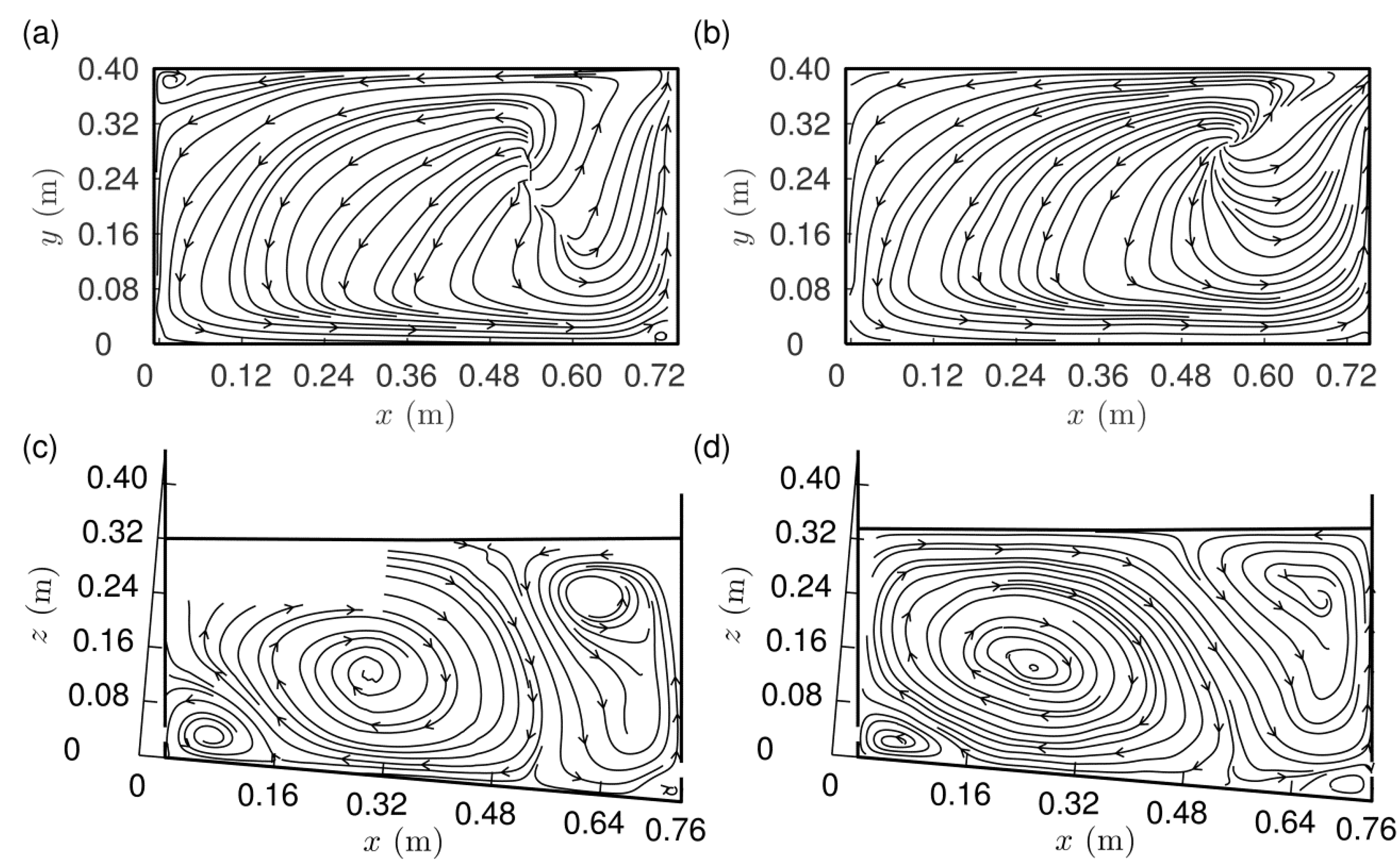
Figure 4 shows the streamlines computed for the time-averaged velocities obtained with the PIV and numerical model mesh A_model in planes 2 and 5. The results from the numerical model are presented only for mesh A_model since no significant differences could be found between mesh A_model and B_model results.

The flow patterns were well predicted by the numerical model, as shown in Figure 4. In plane 2, the jet flow trajectory and width were well captured, and the recirculation zones’ location and size were in good agreement in both planes.

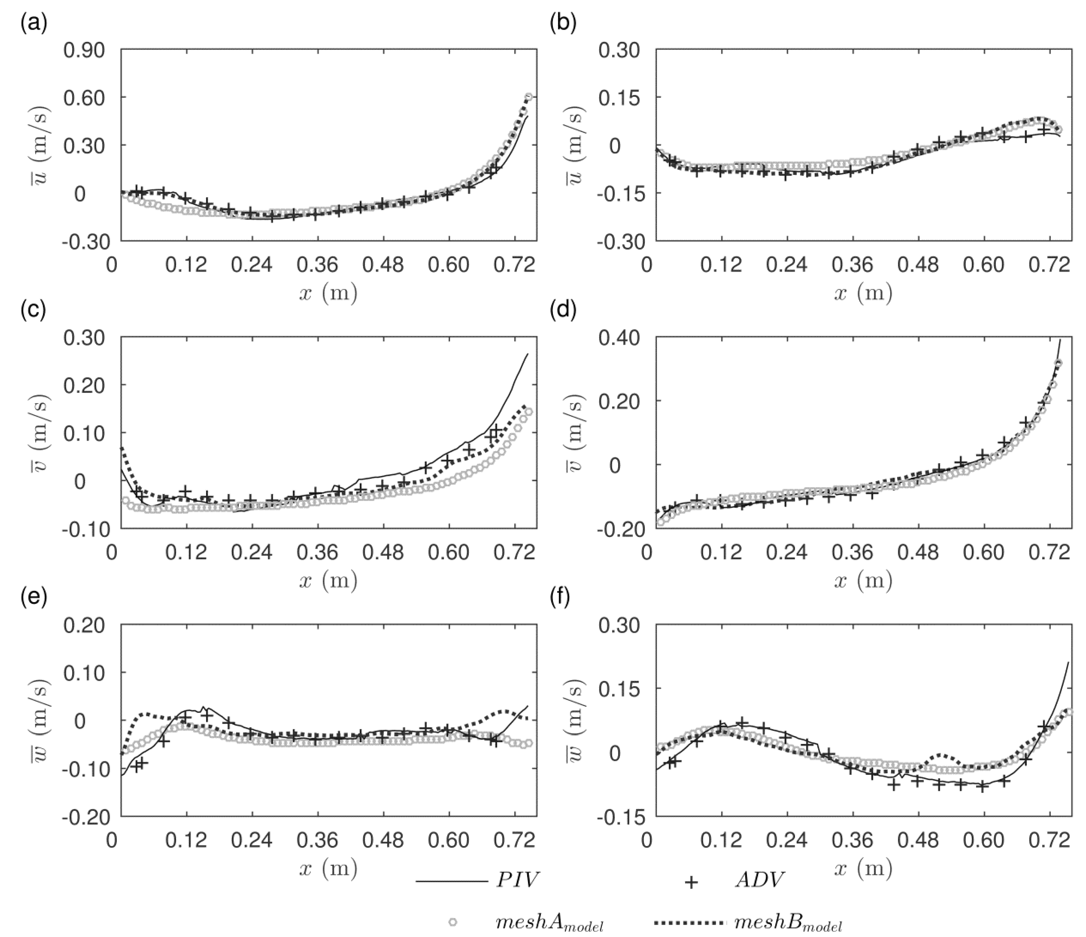
Figure 5 shows the longitudinal variation in the time-averaged velocity components $\overline{\mathrm{u}}$, $\overline{\mathrm{v}}$, and $\overline{\mathrm{w}}$ at two locations. One in the centre of the downstream orifice at planes 1 and 6 intersection (y = 0.36 m and z = 0.04 m), and the other one at the flume centre at planes 2 and 5 intersection (y = 0.20 m and z = 0.088 m). These profiles were chosen because of the high probability of fish being present at these regions, with the first location going through the entrance jet of the pool (considering fish moving upstream) and the second one going through the recirculation zones.

A very good agreement between the experimental and numerical results can be observed in Figure 5 for all the velocity components with the largest differences, that are still acceptable, occurring for values close to 0 of the transversal (Figure 5c) and vertical velocity components (Figure 5e,f).

Figure 6 shows the longitudinal variation in the Reynolds normal stress components $\left(\overline{{{\mathrm{u}}^{\prime }}^2}, \overline{{{\mathrm{v}}^{\prime }}^2,} \mathrm{and} \overline{{{\mathrm{w}}^{\prime }}^2}\right)$ and of the Reynolds shear stress component parallel to the bottom (τ_uv) at the same locations of Figure 5.

Additionally, a good agreement between the experimental and numerical results was found for the turbulence parameters, although not as good as that of the velocity components (Figure 6). The largest differences occurred for the Reynolds shear stress. Nevertheless, for the correlation with fish behaviour in other experimental studies, these differences are considered acceptable. Regarding the transversal and vertical Reynolds normal stress components, a better agreement between Mesh B_model results and the experimental data was observed (Figure 6d–f).

Scale Effects

To analyse the scale effects, the prototype scale numerical model results were analysed and compared to the experimental data, scaled according to the Froude similarity.

The flow depths and discharges differences between the numerical model and the experiments slightly decreased for the prototype scale with average values of 3.4 and 4.8% for mesh A_prototype and 2.3 and 4.1% for mesh B_prototype, for flow depths and discharges, respectively.

Table 4. Comparison between numerical model results at prototype scale and measurements.

		ADV—Numerical Model		PIV—Numerical Model
		ADV—Aprototype	ADV—Bprototype	PIV—Aprototype	PIV—Bprototype
$\overline{\mathrm{u}}$	Nº points a	840		15,884	63,820
	MAD (ms−1)	0.054	0.062	0.058	0.069
	R2	0.92	0.91	0.92	0.92
	dr	0.86	0.84	0.88	0.86
$\overline{\mathrm{v}}$	Nº points a	840		8963	35,852
	MAD (ms−1)	0.035	0.036	0.033	0.033
	R2	0.90	0.87	0.91	0.90
	dr	0.82	0.81	0.83	0.84
$\overline{\mathrm{w}}$	Nº points a	840		6921	27,968
	MAD (ms−1)	0.049	0.042	0.051	0.041
	R2	0.75	0.76	0.75	0.80
	dr	0.69	0.73	0.72	0.77
$\overline{\mathrm{U}}$	Nº points a	840		b
	MAD (ms−1)	0.051	0.062
	R2	0.84	0.80
	dr	0.78	0.74
$\overline{{{\mathrm{u}}^{\prime }}^2}$	Nº points a	840		15,884	63,820
	MAD (m2s−2)	0.0073	0.0085	0.0095	0.0082
	R2	0.80	0.72	0.72	0.75
	dr	0.80	0.77	0.78	0.82
$\overline{{{\mathrm{v}}^{\prime }}^2}$	Nº points a	840		8963	35,852
	MAD (m2s−2)	0.0061	0.0052	0.0074	0.0060
	R2	0.47	0.81	0.38	0.75
	dr	0.72	0.77	0.69	0.75
$\overline{{{\mathrm{w}}^{\prime }}^2}$	Nº points a	840		6921	27,968
	MAD (m2s−2)	0.0057	0.0043	0.0076	0.0064
	R2	0.58	0.80	0.49	0.83
	dr	0.64	0.63	0.74	0.78
κ	Nº points a	840		b
	MAD (m2s−2)	0.0064	0.0075
	R2	0.77	0.82
	dr	0.83	0.80
τuv	Nº points a	840		8963	35,852
	MAD (m2s−2)	2.9	3.3	3.3	3.7
	R2	0.65	0.68	0.58	0.62
	dr	0.78	0.75	0.70	0.67

^a Total number of points compared. ^b Since the PIV measurements were performed with a 2D PIV system this parameter could not be computed.

shows the mean absolute difference (MAD), the coefficient of determination (R²), and refined index of agreement (d_r) for both meshes.

Comparing Table 3 with Table 4, there is no evidence of scale effects; the model performed with similar accuracy for both physical model and prototype dimensions. Only for Reynolds shear stress, a slightly better agreement exists at prototype scale, for the other parameters the agreement is similar.

4. Discussion

Most of the previous numerical modelling studies on fishways relied only upon qualitative comparison of model predictions with experimental or field measurements (e.g., [25,26,27,28,29,30]) and only a few assessed turbulence parameters. As stated by Fuentes-Pérez et al. [35], finding numerical validation data in fishway studies is rather difficult, especially for turbulence metrics. However, Lane and Richards [70] stated that a qualitative assessment of the model predictions is not enough, as velocity measurements represent a sample of a much richer flow field.

Table 3 and Table 4 presented a quantitative statistical comparison between the results obtained with the numerical model and the experimental data obtained with the ADV and the PIV in a laboratory physical model.

The values obtained for MAD, R², and d_r showed an overall good agreement between the numerical results and the experimental data. The best agreement was achieved for the longitudinal and transversal velocity components ($\overline{\mathrm{u}}$ and $\overline{\mathrm{v}}$) and velocity magnitude ($\overline{\mathrm{U}}$), with similar or better agreements relatively to previous studies on open channel flows (e.g., [71,72,73,74,75,76]). Additionally, good agreements were found in the vertical velocity component ($\overline{\mathrm{w}}$), turbulent kinetic energy (κ), and longitudinal Reynolds normal stress $\left(\overline{{{\mathrm{u}}^{\prime }}^2}\right)$. A lower correlation was reported by several authors for $\overline{\mathrm{w}}$ (e.g., [71,72,73,74,75,76]), since vertical velocities are typically very small. In addition, weaker agreements were found for the turbulent kinetic energy, since it involves second-order moment turbulence statistics [76].

For the transversal and vertical Reynolds normal stresses $\left(\overline{{{\mathrm{v}}^{\prime }}^2} \mathrm{and} \overline{{{\mathrm{w}}^{\prime }}^2}\right)$, the agreement obtained for meshes A_model and A_prototype was relatively weak. For meshes B_model and B_prototype, the agreement was much higher and similar to the ones obtained in the vertical velocity, turbulent kinetic energy, and longitudinal Reynolds normal stress. This highlights the importance of validating the numerical model for all the analysed parameters and not only for the most common ones (e.g., discharge, flow depths, and mean velocity).

The weakest agreement, although still acceptable, was obtained for the Reynolds shear stress (τ_uv). This is not surprising since this is a third-order statistical moment, where measurements’ uncertainties become more significant. At prototype scale, the agreement slightly improved. Reynolds normal stress and Reynolds shear stress comparison between experimental data and numerical results were seldom performed. It is worth mentioning that the agreement and differences observed for meshes A_prototype and B_prototype are in accordance with the values observed by Fuentes-Pérez et al. [35] for a vertical slot fishway flow.

The accuracy shown by the numerical model was similar for the prototype and for the physical model, showing no evidence of scale effects. Dargahi [45] used FLOW 3D^® to simulate the flow through a bottom outlet with a moving gate in two different scales, the prototype scale and a 1:22 physical model scale, and it also observed that the model performed with similar accuracy for both scales.

The results attest the ability of the numerical model to adequately characterize the complex flow field of a pool-type fishway with bottom orifices. Although no perfect match between the numerical model predictions and the experimental velocities and turbulence data was found, the agreement was generally better or comparable with what has been regarded as acceptable in previous studies on open channel flows (e.g., [71,72,73,74,75,76]) and fishways [35]. As the experimental data used in the present study was much more extensive (with two experimental measurement techniques used and a much higher number of points compared than in previous studies), with the flow field being more complex, the confidence to use such numerical models for modelling fish passes hydrodynamics is strengthened.

It is also important to mention that the numerical meshes used have a good compromise between accuracy and computational cost. The simulations were performed in a quite accessible computer (Table 1), and the run times for meshes A and B needed to obtain converged time-averaged values is of the order of some days, which is compatible with practical applications.

It is important to emphasize that to accurately reproduce this complex flow field, especially the turbulence parameters, LES model should be used. The lower performance of RNG, k-ε, and k-ω turbulence models in adequately reproducing this flow field, namely, the two last ones, to predict the sizes and shapes of the recirculation zones, may result from the isotropic eddy viscosity assumption and from improperly accounting for the interaction between swirl and turbulence. In this flow field the energy dissipation rate is higher adjacent to the jet. Energy is rapidly dissipated as the jet progresses along the pool. This rapid decay is caused by the entrainment of the recirculating flow on both sides of the jet.

It should also be mentioned that, although in this flow field wall friction does not play an important role, since turbulence production due to wall friction is low when compared to horizontal shear production, as found in other studies [26,27,29], the roughness effect of the walls and bed may be changed by considering different roughness heights. If substrate or bottom macro-roughness’s are added, these can also be represented by using a smaller sized cell in those locations.

In designing an efficient pool-type fishway, one should consider several relevant hydrodynamic variables, such as velocity, flow depth, turbulence, and flow patterns in the pool [2,4,5,6,7,8,9,10,11,12]. Results show that the numerical model accurately predicted these hydrodynamic variables. The flow field in this study mimics real conditions: the prototype numerical model is a real-scaled model based on an indoor full-scale prototype fishway configuration in which tests with fishes (the Iberian barbel) were performed [7,38]. In this study, we chose to analyse one of the configurations used in Silva et al. [38] that proved to be effective for the Iberian barbel, a large-bodied potamodromous benthic cyprinid. Pool-type fishway flows are subcritical flows controlled by the downstream water depth; thus, for a given configuration and slope, when fixing the pool mean water depth only one flow discharge assures uniform flow in the fishway guaranteeing the same hydraulic conditions in every pool, which are the ideal conditions [35] to maximize fishway efficiency. Since Silva et al. [7,39] found that the Reynolds shear stress was the turbulent parameter that most strongly influences the movements of Iberian barbel, the ability of the numerical model to accurately predict this parameter was also assessed in this study, which was not considered in previous fishway numerical modelling studies.

Considering that the flow parameters will be ultimately used for a correlation with fish behaviour, the differences are considered quite acceptable since fish behaviour uncertainties are normally much larger. Thus, it may be concluded that CFD models, namely FLOW 3D^®, can be an adequate and efficient tool to investigate and design pool-type fishways, even with complex flow patterns, such as the ones found in pool-type fishways with bottom orifices. Further research may include the 3D numerical modelling of different basin dimensions and cross-walls configurations.

5. Conclusions

In this study, two distinct measurement techniques, ADV and PIV, were used to measure instantaneous velocities in a laboratory pool-type fishway facility, which is a 1:2.5 physical model of an indoor prototype size pool-type fishway. The experimental data was compared with a 3D numerical model.

Several hydrodynamic variables relevant for fishway analyses and design, such as flow depths, time-averaged velocities, and turbulence parameters (namely, turbulent kinetic energy, Reynolds normal stresses, and Reynolds shear stress component parallel to the bottom), were determined and compared. The results highlighted the importance of validating the numerical model for all the parameters under analyses.

A good agreement between the numerical model and the experimental data was achieved, showing the ability of the numerical model to adequately reproduce the complex flow field of a pool-type fishway with bottom orifices. In addition, no scale effects were observed in the numerical modelling, which presented similar accuracy for near-prototype and physical model scales. Therefore, since the used numerical meshes have a good compromise between accuracy and computational cost, we consider that 3D CFD models, namely FLOW 3D^®, may be successfully used to simulate the pool-type fishway hydrodynamics, constituting a valuable tool to analyse and design fishways, allowing to eliminate and/or complement physical model testing. This could greatly improve fishways design process, as new configurations or different solutions for retrofitting existing nonoperational fishways could be tested and optimized in shorter periods, and in a less expensive way prior to their construction.

References

- Santos, J.M.; Branco, P.J.; Silva, A.T.; Katopodis, C.; Pinheiro, A.N.; Viseu, T.; Ferreira, M.T. Effect of two flow regimes on the upstream movements of the Iberian barbel (Luciobarbus bocagei) in an experimental pool-type fishway. J. Appl. Ichthyol. 2012, 29, 425–430. [Google Scholar] [CrossRef]
- Williams, J.G.; Armstrong, G.; Katopodis, C.; Larinier, M.; Travade, F. Thinking like a fish: A key ingredient for development of effective fish passage facilities at river obstructions. River Res. Appl. 2012, 28, 407–417. [Google Scholar] [CrossRef] [Green Version]
- Noonan, M.J.; Grand, J.W.A.; Jackson, C.D. A quantitative assessment of fish passage efficiency. Fish Fish. 2012, 13, 450–464. [Google Scholar] [CrossRef]
- Haro, A.; Kynard, B. Video Evaluation of Passage Efficiency of American Shad and Sea Lamprey in a Modified Ice Harbor Fishway. N. Am. J. Fish. Manag. 1997, 17, 981–987. [Google Scholar] [CrossRef]
- Odeh, M.; Noreika, J.F.; Haro, A.; Maynard, A.; Castro-Santos, T. Evaluation of the Effects of Turbulence on the Behavior of Migratory Fish; Contract no. 00000022, Project no. 200005700 (BPA Report DOE/BP-00000022-1); Report to the Bonneville Power Administration: Portland, Oregon, 2002. [Google Scholar]
- Enders, E.C.; Boisclair, D.; Roy, A.G. The effect of turbulence on the cost of swimming for juveniles of Atlantic Salmon (Salmo salar). Can. J. Fish. Aquat. Sci. 2003, 60, 1149–1160. [Google Scholar] [CrossRef]
- Silva, A.T.; Santos, J.M.; Ferreira, M.T.; Pinheiro, A.N.; Katopodis, C. Effects of water velocity and turbulence on the behaviour of Iberian barbel (Luciobarbus bocagei, Steindachner, 1864) in an experimental pool-type fishway. River Res. Appl. 2011, 27, 360–373. [Google Scholar] [CrossRef]
- Silva, A.T.; Katopodis, C.; Santos, J.M.; Ferreira, M.T.; Pinheiro, A.N. Cyprinid swimming behaviour in response to turbulent flow. Ecol. Eng. 2012, 44, 314–328. [Google Scholar] [CrossRef] [Green Version]
- Lacey, R.W.J.; Neary, V.S.; Liao, J.C.; Enders, E.C.; Tritico, H.M. The IPOS framework: Linking fish swimming performance in altered flows from laboratory experiments to rivers. River Res. Appl. 2012, 28, 429–443. [Google Scholar] [CrossRef]
- Santos, J.M.; Silva, A.T.; Katopodis, C.; Pinheiro, P.J.; Pinheiro, A.N.; Bochechas, J.; Ferreira, M.T. Ecohydraulics of pool-type fishways: Getting past the barriers. Ecol. Eng. 2012, 48, 38–50. [Google Scholar] [CrossRef]
- Branco, P.J.; Santos, J.M.; Katopodis, C.; Pinheiro, A.N.; Ferreira, M.T. Effect of flow regime hydraulics on passage performance of Iberian chub (Squalius pyrenaicus) (Günther, 1868) in an experimental pool-and-weir fishway. Hydrobiologia 2013, 714, 145–154. [Google Scholar] [CrossRef]
- Gao, Z.; Andersson, H.I.; Dai, H.; Jiang, F.; Zhao, L. A new Eulerian-Lagrangian agent method to model fish paths in a vertical slot fishways. Ecol. Eng. 2016, 88, 217–225. [Google Scholar] [CrossRef] [Green Version]
- Rajaratnam, N.; Katopodis, C.; Mainali, M. Pool-orifice and pool-orifice-weir fishways. Can. J. Civ. Eng. 1989, 16, 774–777. [Google Scholar] [CrossRef]
- Wu, S.; Rajaratnam, N.; Katopodis, C. Structure of flow in vertical slot fishway. J. Hydraul. Eng. 1999, 125, 351–360. [Google Scholar] [CrossRef]
- Kim, J.H. Hydraulic characteristics by weir type in a pool-weir fishway. Ecol. Eng. 2001, 16, 425–433. [Google Scholar] [CrossRef]
- Ead, S.A.; Katopodis, C.; Sikora, G.J.; Rajaratnam, N. Flow regimes and structure in pool and weir fishways. J. Environ. Eng. Sci. 2004, 3, 379–390. [Google Scholar] [CrossRef] [Green Version]
- Puertas, J.; Pena, L.; Teijeiro, T. Experimental approach to the hydraulics of vertical slot fishways. J. Hydraul. Eng. 2004, 130, 10–23. [Google Scholar] [CrossRef]
- Liu, M.; Rajaratnam, N.; Zhu, D.D. Mean flow and turbulence structure in vertical slot fishways. J. Hydraul. Eng. 2006, 132, 765–777. [Google Scholar] [CrossRef]
- Yagci, O. Hydraulic aspects of pool-weir fishways as ecologically friendly water structure. Ecol. Eng. 2010, 36, 36–46. [Google Scholar] [CrossRef]
- Tarrade, L.; Pineau, G.; Calluaud, D.; Texier, A.; David, L.; Larinier, M. Detailed experimental study of hydrodynamic turbulent flows generated in vertical slot fishways. Environ. Fluid Mech. 2011, 11, 1–21. [Google Scholar] [CrossRef] [Green Version]
- Calluaud, D.; Pineau, G.; Texier, A.; David, L. Modification of vertical slot fishway flow with a supplementary cylinder. J. Hydraul. Res. 2014, 52, 614–629. [Google Scholar] [CrossRef]
- Ballu, A.; Calluaud, D.; Pineau, G.; David, L. Experimental study of the influence of macro-roughnesses on vertical slot fishway flows. La Houille Blanche 2017, 2, 9–14. [Google Scholar] [CrossRef]
- Blocken, B.; Gualtieri, C. Ten iterative steps for model development and evaluation applied to computational fluid dynamics for environmental fluid mechanics. Environ. Model. Softw. 2012, 33, 1–22. [Google Scholar] [CrossRef]
- Zhang, J.; Tejada-Martínez, A.E.; Zhang, Q. Developments in computational fluid dynamics-based modeling for disinfection technologies over the last two decades: A review. Environ. Model. Softw. 2014, 58, 71–85. [Google Scholar] [CrossRef]
- Khan, L.A. A Three-Dimensional Computational Fluid Dynamics (CFD) Model Analysis of Free Surface Hydrodynamics and Fish Passage Energetics in a Vertical-Slot Fishway. N. Am. J. Fish. Manag. 2006, 26, 255–267. [Google Scholar] [CrossRef]
- Cea, L.; Pena, L.; Puertas, J.; Vazquez-Cendon, M.E.; Peña, E. Application of several depth-averaged turbulence models to simulate flow in vertical slot fishways. J. Hydraul. Eng. 2007, 133, 160–172. [Google Scholar] [CrossRef]
- Barton, A.F.; Keller, R.J.; Katopodis, C. Verification of a numerical model for the prediction of low slope vertical slot fishway hydraulics. Aust. J. Water Res. 2009, 13, 53–60. [Google Scholar] [CrossRef]
- Chorda, J.; Maubourguet, M.M.; Roux, H.; George, J.; Larinier, M.; Tarrade, L.; David, L. Two-dimensional free surface flow numerical model for vertical slot fishways. J. Hydraul. Res. 2010, 48, 141–151. [Google Scholar] [CrossRef] [Green Version]
- Bombač, M.; Novak, G.; Rodič, P.; Četina, M. Numerical and physical model study of a vertical slot fishway. J. Hydrol. Hydromech. 2014, 62, 150–159. [Google Scholar] [CrossRef] [Green Version]
- Bombač, M.; Novak, G.; Mlacnik, J.; Četina, M. Extensive field measurements of flow in vertical slot fishway as data for validation of numerical simulations. Ecol. Eng. 2015, 84, 476–484. [Google Scholar] [CrossRef]
- Bombač, M.; Četina, M.; Novak, G. Study on flow characteristics in vertical slot fishways regarding slot layout optimization. Ecol. Eng. 2017, 107, 126–136. [Google Scholar] [CrossRef]
- Marriner, B.A.; Baki, A.B.M.; Zhu, D.Z.; Thiem, J.D.; Cooke, S.J.; Katopodis, C. Field and numerical assessment of turning pool hydraulics in a vertical slot fishway. Ecol. Eng. 2014, 63, 88–101. [Google Scholar] [CrossRef]
- Marriner, B.A.; Baki, A.B.M.; Zhu, D.Z.; Cooke, S.J.; Katopodis, C. The hydraulics of a vertical slot fishway: A case study on the multi-species Vianney-Legendre fishway in Quebec, Canada. Ecol. Eng. 2016, 90, 190–202. [Google Scholar] [CrossRef]
- Quaranta, E.; Katopodis, C.; Revelli, R.; Comoglio, C. Turbulent flow field comparison and related suitability for fish passage of a standard and a simplified low-gradient vertical slot fishway. River Res. Appl. 2017, 33, 1295–1305. [Google Scholar] [CrossRef]
- Fuentes-Pérez, J.F.; Silva, A.T.; Tuhtan, J.A.; García-Vega, A.; Carbonell-Baeza, R.; Musall, M.; Kruusmaa, M. 3D modelling of non-uniform and turbulent flow in vertical slot fishways. Environ. Model. Softw. 2018, 99, 156–169. [Google Scholar] [CrossRef]
- Stamou, A.; Mitsopoulos, G.; Rutschmann, P.; Bui, M. Verification of a 3D CFD model for vertical slot fish-passes. Environ. Fluid Mech. 2018, 18, 1435–1461. [Google Scholar] [CrossRef]
- Sanagiotto, D.; Rossi, J.; Bravo, J. Applications of computational fluid dynamics in the design and rehabilitation of nonstandard vertical slot fishways. Water 2019, 11, 199. [Google Scholar] [CrossRef] [Green Version]
- Silva, A.T.; Santos, J.M.; Franco, A.C.; Ferreira, M.T.; Pinheiro, A.N. Selection of Iberian barbel Barbus bocagei (Steindachner, 1864) for orifices and notches upon different hydraulic configurations in an experimental pool-type fishway. J. Appl. Ichthyol. 2009, 25, 173–177. [Google Scholar] [CrossRef]
- Silva, A.T.; Santos, J.M.; Ferreira, M.T.; Pinheiro, A.N.; Katopodis, C. Passage efficiency of offset and straight orifices for upstream movements of Iberian barbel in a pool-type fishway. River Res. Appl. 2012, 28, 529–542. [Google Scholar] [CrossRef]
- Branco, P.; Santos, J.M.; Katopodis, C.; Pinheiro, A.; Ferreira, M.T. Pool-Type Fishways: Two Different Morpho-Ecological Cyprinid Species Facing Plunging and Streaming Flows. PLoS ONE 2013, 8, e65089. [Google Scholar] [CrossRef]
- Romão, F.; Quaresma, A.L.; Branco, P.; Santos, J.M.; Amaral, S.; Ferreira, M.T.; Katopodis, C.; Pinheiro, A.N. Passage performance of two cyprinids with different ecological traits in a fishway with distinct vertical slot configurations. Ecol. Eng. 2017, 105, 180–188. [Google Scholar] [CrossRef] [Green Version]
- Romão, F.; Branco, P.; Quaresma, A.L.; Amaral, S.; Pinheiro, A.N. Effectiveness of a multi-slot vertical slot fishway versus a standard vertical slot fishway for potamodromous cyprinids. Hydrobiologia 2018, 816, 153–163. [Google Scholar] [CrossRef]
- Romão, F.; Quaresma, A.L.; Santos, J.M.; Branco, P.; Pinheiro, A.N. Cyprinid passage performance in an experimental multislot fishway across distinct seasons. Mar. Freshw. Res. 2019, 70, 881–890. [Google Scholar] [CrossRef]
- Haque, M.M.; Constantinescu, G.; Weber, L. Validation of a 3D RANS model to predict flow and stratification effects related to fish passage at hydropower dams. J. Hydraul. Res. 2007, 45, 787–796. [Google Scholar] [CrossRef]
- Dargahi, B. Flow characteristics of bottom outlets with moving gates. J. Hydraul. Res. 2010, 48, 476–482. [Google Scholar] [CrossRef]
- Huang, W.; Yang, Q.; Xiao, H. CFD modelling of scale effects on turbulence flow and scour around bridge piers. Comput. Fluids 2009, 38, 1050–1058. [Google Scholar] [CrossRef]
- Heller, V. Scale effects in physical hydraulic engineering models. J. Hydraul. Res. 2011, 49, 293–306. [Google Scholar] [CrossRef]
- Larinier, M. Pool fishways, pre-barrages and natural bypass channels. Bull. Français de la Pêche et de la Piscic. 2002, 364, 54–82. [Google Scholar] [CrossRef] [Green Version]
- Quaresma, A.L.; Ferreira, R.M.L.; Pinheiro, A.N. Comparative analysis of particle image velocimetry and acoustic Doppler velocimetry in relation to a pool-type fishway flow. J. Hydraul. Res. 2017, 55, 582–591. [Google Scholar] [CrossRef]
- Flow Science, Inc. Flow-3D Version 11.2 User Manual; Flow Science, Inc.: Los Alamos, NM, USA, 2016. [Google Scholar]
- Hirt, C.W.; Sicilian, J.M. A porosity technique for the definition of obstacles in rectangular cell meshes. In Proceedings of the International Conference on Numerical Ship Hydrodynamics, Washington, DC, USA, 4 September 1985. [Google Scholar]
- Savage, B.M.; Johnson, M.C. Flow over ogee spillway: Physical and numerical model case study. J. Hydraul. Eng. 2001, 127, 640–649. [Google Scholar] [CrossRef]
- Abad, J.D.; Rhoads, B.L.; Güneralp, I.; García, M.H. Flow structure at different stages in a meander-bend with bendway weirs. J. Hydraul. Eng. 2008, 134, 1052–1063. [Google Scholar] [CrossRef]
- Bombardelli, F.A.; Meireles, I.; Matos, J. Laboratory measurements and multi-block numerical simulations of the mean flow and turbulence in the non-aerated skimming flow region of steep stepped spillways. Environ. Fluid Mech. 2011, 11, 263–288. [Google Scholar] [CrossRef] [Green Version]
- Bayon, A.; Valero, D.; García-Bartual, R.; López-Jiménez, P.A. Performance assessment of OpenFOAM and FLOW-3D in the numerical modeling of a low Reynolds number hydraulic jump. Environ. Model. Softw. 2016, 80, 322–335. [Google Scholar] [CrossRef]
- Duguay, J.M.; Lacey, R.W.J.; Gaucher, J. A case study of a pool and weir fishway modeled with OpenFOAM and FLOW-3D. Ecol. Eng. 2017, 103, 31–42. [Google Scholar] [CrossRef]
- Hirt, C.W.; Nichols, B.D. Volume of fluid (VOF) method for the dynamics of free boundaries. J. Comp. Phys. 1981, 39, 201–225. [Google Scholar] [CrossRef]
- Van Leer, B. Towards the ultimate conservative difference scheme. IV. A new approach to numerical convection. J. Comp. Phys. 1977, 23, 276–299. [Google Scholar] [CrossRef]
- Celik, I.B.; Ghia, U.; Roache, P.J.; Freitas, C.J.; Coleman, H.; Raad, P.E. Procedure for Estimation and Reporting of Uncertainty Due to Discretization in CFD Applications. J. Fluids Eng. 2008, 130, 078001 (4pages). [Google Scholar] [CrossRef] [Green Version]
- Smagorinsky, J. General circulation experiments with the primitive equations: I. The Basic Experiment. Mon. Weather Rev. 1963, 91, 99–164. [Google Scholar] [CrossRef]
- Meyers, J.; Geurts, B.J.; Baelmans, M. Database analysis of errors in large-eddy simulation. Phys. Fluids 2003, 15, 2740–2755. [Google Scholar] [CrossRef] [Green Version]
- Celik, I.B.; Cehreli, Z.N.; Yavuz, I. Index of Resolution Quality for Large Eddy Simulations. J. Fluids Eng. 2005, 127, 949–958. [Google Scholar] [CrossRef]
- Freitag, M.; Klein, M. An improved method to assess the quality of large eddy simulations in the context of implicit filtering. J. Turbul. 2006, 7, 1–11. [Google Scholar] [CrossRef]
- Gousseau, P.; Blocken, B.; van Heijst, G.J.F. Quality assessment of Large-Eddy Simulation of wind flow around a high-rise building: Validation and solution verification. Comput. Fluids 2013, 79, 120–133. [Google Scholar] [CrossRef]
- Celik, I.; Li, J.; Hu, G.; Shaffer, C. Limitations of Richardson Extrapolation and Some Possible Remedies. J. Fluids Eng. 2005, 127, 795–805. [Google Scholar] [CrossRef]
- Pope, S.B. Turbulent Flows; Cambridge University Press: Cambridge, UK, 2000. [Google Scholar]
- Legates, D.R.; McCabe, G.J., Jr. Evaluating the use of “goodness-of-fit” Measures in hydrologic and hydroclimatic model validation. Water Resour. Res. 1999, 35, 233–241. [Google Scholar] [CrossRef]
- Bennett, N.D.; Crok, B.F.W.; Guariso, G.; Guillaume, J.H.A.; Hamilton, S.H.; Jakeman, A.J.; Marsili-Libelli, S.; Newhama, L.T.H.; Norton, J.P.; Perrin, C.; et al. Characterising performance of environmental models. Environ. Model. Softw. 2013, 40, 1–20. [Google Scholar] [CrossRef]
- Willmott, C.J.; Robeson, S.M.; Matsuura, K. A refined index of model performance. Int. J. Climatol. 2012, 32, 2088–2094. [Google Scholar] [CrossRef]
- Lane, S.N.; Richards, K.S. The “validation” of hydrodynamic models: Some critical perspectives. In Model Validation for Hydrological and Hydraulic Research; Bates, P.D., Anderson, M.G., Eds.; John Wiley: Hoboken, NJ, USA, 2001; pp. 413–438. [Google Scholar]
- Bradbrook, K.F.; Biron, P.M.; Lane, S.N.; Richards, K.S.; Roy, A.G. Investigation of controls on secondary circulation in a simple confluence geometry using a three-dimensional numerical model. Hydrol. Process. 1998, 12, 1371–1396. [Google Scholar] [CrossRef]
- Bradbrook, K.F.; Lane, S.N.; Richards, K.S.; Biron, P.M.; Roy, A.G. Role of bed discordance at asymmetrical river confluences. J. Hydraul. Eng. 2001, 127, 351–368. [Google Scholar] [CrossRef]
- Ferguson, R.I.; Parsons, D.R.; Lane, S.N.; Hardy, R.J. Flow in meander bends with recirculation at the inner bank. Water Resour. Res. 2003, 39, 1322–1334. [Google Scholar] [CrossRef] [Green Version]
- Haltigin, T.W.; Biron, P.M.; Lapointe, M.F. Predicting equilibrium scour-hole geometry near angled stream deflectors using a three-dimensional numerical flow model. J. Hydraul. Eng. 2007, 133, 983–988. [Google Scholar] [CrossRef]
- Haltigin, T.W.; Biron, P.M.; Lapointe, M.F. Three-dimensional numerical simulation of flow around stream deflectors: The effects of obstruction angle and length. J. Hydraul. Res. 2007, 45, 227–238. [Google Scholar] [CrossRef]
- Han, S.S.; Biron, P.M.; Ramamurthy, A.S. Three-dimensional modelling of flow in sharp open-channel bends with vanes. J. Hydraulic Res. 2011, 49, 64–72. [Google Scholar] [CrossRef]
- Klein, M. An Attempt to assess the quality of large eddy simulations in the context of implicit filtering. Flow Turbul. Combust. 2005, 75, 131–147. [Google Scholar] [CrossRef]
Figure 1.
Experimental flume used (a) Side view of the flume; (b) Pool detail.
Figure 2.
Three dimensional representations of a pool showing the measurement planes and the acoustic Doppler velocimetry (ADV) measurement grid (a) measurement planes parallel to the flume bottom; (b) vertical measurement planes (ADV measurement grid is only shown in one plane).
Figure 3.
Computational domain, showing Pool 3 mesh block.
Figure 4.
Streamlines of time-averaged velocities (left: PIV; right: mesh Amodel): (a,b) plane 2 (z = 0.088 m); (c,d) plane 5 (y = 0.20 m).
Figure 5.
Longitudinal variation of velocity components: (a,c,e) planes 1 and 6 intersection (y = 0.36 m and z = 0.04 m); (b,d,f) planes 2 and 5 intersection (y = 0.20 m and z = 0.088 m).
Figure 6.
Longitudinal variation of Reynolds normal stress components and Reynolds shear stress parallel to the bottom component: (a,c,e,g) planes 1 and 6 intersection (y = 0.36 m and z = 0.04m); (b,d,f,h) planes 2 and 5 intersection (y = 0.20 m and z = 0.088 m).