
Accounting for Uncertainties in the Safety Assessment of Concrete Gravity Dams: A Probabilistic Approach with Sample Optimization


1
Department of Civil Engineering and Building Engineering, University of Sherbrooke, Sherbrooke, QC J1K 2R1, Canada
2
Dam Expertise Unit, Hydro-Quebec, Montréal, QC H2Z 1A4, Canada
3
Department of Civil and Environmental Engineering, Rice University, Houston, TX 77005, USA
*
Author to whom correspondence should be addressed.
Water 2021, 13(6), 855; https://doi.org/10.3390/w13060855
Submission received: 25 January 2021
/
Revised: 8 March 2021
/
Accepted: 15 March 2021
/
Published: 20 March 2021
(This article belongs to the Special Issue Soft Computing and Machine Learning in Dam Engineering)
Abstract
:Important advances have been made in the methodologies for assessing the safety of dams, resulting in the review and modification of design guidelines. Many existing dams fail to meet these revised criteria, and structural rehabilitation to achieve the updated standards may be costly and difficult. To this end, probabilistic methods have emerged as a promising alternative and constitute the basis of more adequate procedures of design and assessment. However, such methods, in addition to being computationally expensive, can produce very different solutions, depending on the input parameters, which can greatly influence the final results. Addressing the existing challenges of these procedures to analyze the stability of concrete dams, this study proposes a probabilistic-based methodology for assessing the safety of dams under usual, unusual, and extreme loading conditions. The proposed procedure allows the analysis to be updated while avoiding unnecessary simulation runs by classifying the load cases according to the annual probability of exceedance and by using an efficient progressive sampling strategy. In addition, a variance-based global sensitivity analysis is performed to identify the parameters most affecting the dam stability, and the parameter ranges that meet the safety guidelines are formulated. It is observed that the proposed methodology is more robust, more computationally efficient, and more easily interpretable than conventional methods.
1. Introduction
Dams are a vital part of the nation’s infrastructure, providing economic, environmental, and social benefits. The benefits of dams, however, are countered by the risks they can present [1]. The structural stability of major dams needs to be re-evaluated every 5–10 years according to hazard classification systems (HCSs), most often within the legal framework of a governmental regulatory agency [2]. Requirements for the stability of concrete dams in the current regulations are based on simplifications, which, in many cases, are very conservative. Concrete dams in Canada, as in most of the world, are designed and assessed based on a deterministic framework using safety factors (SFs). Although the failure rate of gravity dams is low, the deterministic approach suffers from several problems, including the equal treatment of loads and the identical consideration of strength and capacity uncertainties, which are combined into a single safety factor. As a consequence, unnecessary rehabilitation works may be carried out on dams that are safe but do not meet the safety requirements. When safety is re-evaluated, it is important that this evaluation is based on modern safety concepts, such as a probabilistic analysis, to support decision-making [3].
In contrast to the deterministic approach, the probabilistic approach requires the treatment of each parameter as a continuous function that associates a probability of occurrence to the distribution. This probability density function (PDF) allows variables to be treated as uncertain inputs by directly incorporating uncertainties into the model evaluation process [4]. The uncertainties are propagated through the system to obtain a quantitative estimate of the probability of exceeding a specific loading scenario or system configuration. Although probabilistic methods have been considered as a promising alternative for the safety assessment of dams, such methods often require a large number of simulations. Moreover, in the context of a probabilistic analysis, new information gained through laboratory tests, in situ tests, empirical observations, etc., could update the prior knowledge assumed for different variables in the PDFs. However, this is frequently overlooked given the costly re-evaluation of these simulations. Innovations, such as the use of machine learning techniques [5,6,7], have been proposed to overcome these drawbacks. However, such procedures can be subject to misinterpretation if not applied correctly due to their complexity. Thus, there is a need to develop simplified and more expeditious methods for analyzing the safety of dams within a probabilistic framework.
To further encourage the applicability of these methods, the main objective of this study is to develop a probabilistic-based methodology to assess the safety of dams that allows analysis updating in light of new information, preventing the need for the re-evaluation of the system simulations. Additionally, an efficient progressive sampling strategy that sequentially generates sample points while progressively preserving the distributional properties of interest is used to optimize the sample size and avoid unnecessary simulation runs. As a result, after the final number of simulation runs is established, variations in the loading conditions are considered by modifying the parameter’s cumulative density function defining the annual probability of exceedance. In this manner, there is no need to re-run simulations when the system’s loading parameters vary. These simulations are then used to estimate the probability of exceeding a target monitored response for a given loading scenario. In the same way, variance-based global sensitivity analyses with progressive complexity are performed to identify the parameters most affecting the dam stability, and ranges of values that satisfy the SFs provided by safety guidelines are formulated. The proposed methodology is applied to a case study gravity dam located in north-eastern Canada.
2. Related Works
In recent decades, the knowledge in the evaluation of natural hazards has evolved considerably, making it necessary to reassess the stability of dams under usual, unusual, and extreme loading. As mentioned above, methods for analyzing the structural stability of a dam system rely on deterministic or probabilistic approaches. Deterministic analysis has traditionally been used to assess the stability of dams [8,9,10,11]. Nevertheless, these methods are often considered overly conservative or even unsafe in some cases because they neglect the different sources of uncertainty and because of the use of extreme load cases with very low probabilities of occurrence [12,13,14]. Thus, there is interest in moving towards more refined methods for considering uncertainties. For these reasons, probabilistic assessment has emerged as a useful tool in dam safety, and the results have been found to be promising by recent studies [2,3,15,16,17,18,19]. However, the use of probabilistic methods for dams within a normative framework is not well developed, but increasing scrutiny is being applied to this field. The most recent guidelines for the design and assessment of gravity dams are now including probabilistic notions for the assessment of these structures [4,14,20,21,22,23,24].
For a reliable probabilistic analysis, the emphasis must be placed on the quality of the input parameters and in particular the uncertainties. However, probabilistic assessment, no matter how sophisticated, can still lead to very different solutions for a given problem because of the complex choices of random variables (RVs), characteristic values, PDFs, and bounds, which can largely influence final results [25,26,27]. Consequently, the analysis is generally not updated in light of new information due to the time-consuming re-evaluation and the lack of flexibility in the methods regarding including modified PDFs and bounds. Indeed, although the information contained in the probabilistic results is far-reaching, it is still currently difficult to carry out an in-depth study to assess the safety of dams according to all scenarios. Accordingly, together with the probabilistic approach, the deterministic method can be used to complement the safety assessment [28]. To this end, a preliminary RV selection phase or sensitivity is sometimes proposed prior to probabilistic analyses. Tornado diagrams (TDs) [29] are an example of the deterministic (or semideterministic if the input variables are PDFs) sensitivity methods that have been widely used for the efficient selection of leading variables [30,31,32,33]. Similarly, more refined methods, such as analysis of variance (ANOVA) and Sobol’s method [34], have been used for assessing the significance of each modeling parameter on the structural responses of dams [17,35,36].
3. Methodology
Probabilistic analysis identifies the uncertainties that are key for safety and attempts to include all plausible scenarios, their likelihood and their consequences. It yields more comprehensive estimates than deterministic analysis due to the range associated with the input variables. However, it is undeniable that deterministic analysis, in terms of SFs, is still the most widely used method for design and assessment in the dam industry [37]. With this in mind, the two approaches are combined in this study to provide a better understanding of the output of a probabilistic analysis in terms of practical considerations.
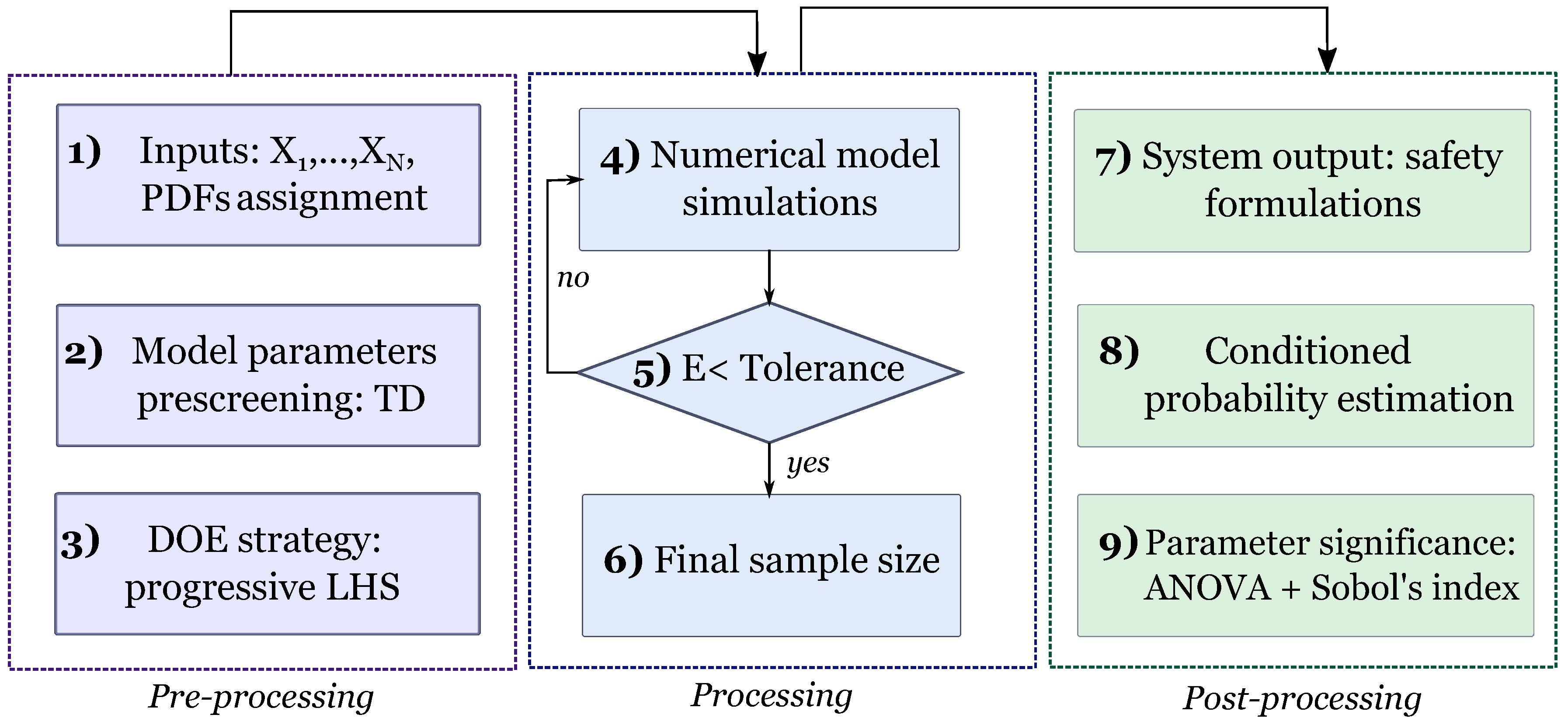
The main steps of the proposed methodology are shown in Figure 1; the methodology is divided into three stages: (i) pre-processing (steps 1–3), (ii) processing (steps 4–6), and (iii) post-processing (steps 6–9). In the pre-processing stage, the load and resistance input parameters that can be considered RVs and their respective PDFs are defined. Next, a prescreening of the model parameter sensitivity is performed by generating TDs to define the final set of RV, PDFs, and maximum and minimum bounds. Then, to optimize the computational resources, a progressive design of experiments (DOE) strategy based on the the progressive Latin hypercube sampling (PLHS) [38] technique is employed. Concerning the processing stage, a numerical model of the system is developed. Subgroups of the total number of simulations are analyzed sequentially, and the error in each iteration is compared to a specific tolerance, which when satisfied, determines the final sample size. Finally, in the post-processing stage, safety recommendations are formulated by evaluating the system output, the probability of exceeding a target performance indicator conditioned on a load combination (LC) is estimated, and ANOVA is performed to assess the global parameter significance while Sobol’s indices are estimated to quantify their importance. In the next sections, each of these steps is explained in detail.
3.1. Sampling Strategy
An efficient sampling strategy that scales with the size of the problem and computational resources is essential for various sampling-based analyses, such as sensitivity and uncertainty analyses. To this end, as the sample size increases, PLHS [38], which sequentially generates sample points while progressively preserving the distributional properties of interest (Latin hypercube properties, space-filling, etc.), is used. PLHS generates a series of smaller subsets (slices) such that (i) the first slice is a Latin hypercube, (ii) the progressive union of slices remains a Latin hypercube and achieves maximum stratification in any one-dimensional projection, and, as such, (iii) the entire sample set is a Latin hypercube. To optimize the sampling size, a maximum number of permitted simulations, , is established. The total number of permitted simulations is then divided into n slices, each containing samples. The simulations are run iteratively, one slice at a time, and the results for each iteration are cumulatively saved. To define the final sample size, the algorithm starts with one slice. In the next step, another slice is added, and the convergence of the algorithm is measured by calculating the relative errors presented in Equations (1)–(3) and comparing them to a tolerance of .
where SSF is the sliding safety factor for the normal load case, is the number of samples per slice, and are the mean safety factors calculated with and n slices, respectively, and is an indicator function, where if , and otherwise. The considered stopping conditions concern the statistics (mean and standard deviation) of the model response in Equations (1) and (2) and the probability of presenting a SSF lower than a given value in Equation (3). It should be noted that in Equation (3), a threshold of 3 is used because the SFs from the usual load case are considered, as will be explained later in Section 4.2. Usually, the convergence of the SSF probability is slower than that of the statistical moments, such that the obtained results could be accurate for the mean and standard deviation, but not for the SSF probability, especially for low probabilities. Therefore, Equations (1)–(3) are used together to evaluate the convergence of the algorithm.
3.2. Sensitivity Analysis
After the selection of the initial set of model parameters that can be considered to be RVs in the analysis, a prescreening is performed by generating TDs to determine the final set. This semideterministic analysis is used to evaluate a broad scenario trade space and narrow the set of options to those that are viable, given the performance, cost, and safety constraints. Because deterministic analysis requires a relatively short computational time, it is possible to rapidly iterate through possible scenarios at this low level of fidelity. However, it is difficult for TDs to evaluate the effect of simultaneous variation in a large number of input parameters on the model output results. To this end, after the simulations, the analysis is expanded, and ANOVA is performed to understand the global parameter significance and to draw inferences about the effect of the joint variation of the parameters on the target output.
3.2.1. Tornado Diagrams
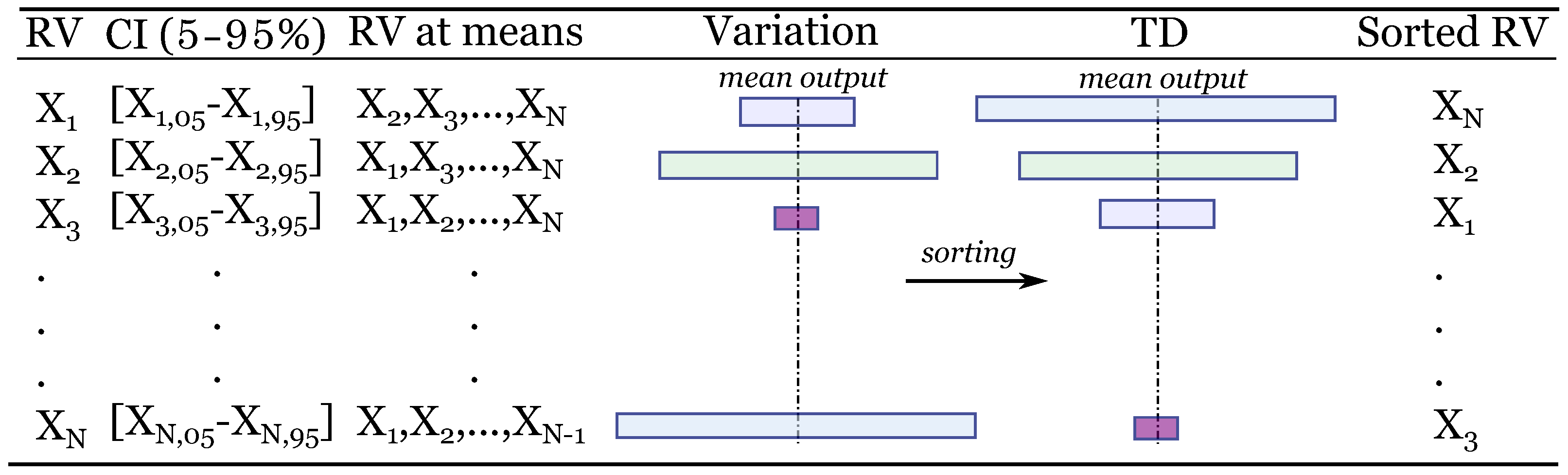
TDs quantify the impact of single RV variations on the target output results. It is also very useful tool to identify which variables are worth resource investment regarding reducing uncertainties. A TD is composed of horizontal bars with widths given by the sensitivity of a specific RV. These bars are sorted vertically from the most influential at the top of the diagram, to the least sensitive at the bottom; thus, the diagram looks like a tornado. Figure 2 presents the methodology, which can be explained as follows: (i) for each RV, the mean value and the 5–95% confidence interval (CI) are determined; (ii) numerical simulations are carried out considering the CI bounds of a single parameter while keeping the remaining parameters at their mean value, i.e., for N input RV, 2N analyses are performed; (iii) the difference in the results of the two extreme values of an RV gives the absolute value of variation. Next, the TD is constructed by sorting the parameters from the greatest to the lowest variation.
3.2.2. Variance-Based Global Sensitivity Analysis
Even though TDs are easily interpretable and visually explicit, they can consider only variation in one parameter at a time, providing only a local sensitivity for each parameter. The concept of using the variance as an indicator of the importance of an input parameter is the basis for many variance-based global sensitivity analysis methods [39]. With this in mind, to evaluate the global significance of each parameter in the structure response by considering their joint variation, a sensitivity study using ANOVA is performed. ANOVA includes hypothesis tests that verify the significance of varying each parameter on the variance of the measured responses [40]. The results of the hypothesis tests are given in terms of a p-value, and a smaller p-value indicates greater evidence that the parameter has a strong influence on the dam response. A typical significance cut-off value of is adopted here. Similarly, Sobol’s method [34], another variance-based global sensitivity analysis, is applied because of its ability to quantify the importance of each input random variable. Sobol’s method uses the decomposition of the variance to calculate the sensitivity indices.
3.3. Conditional Probability of Exceedance Estimation
Safety is subjective and is a matter of addressing public concern as specified in safety guidelines or regulations [15]. For the case of a deterministic analysis, this implies equating the SF to a formalized target criterion tolerated by the profession and society. With the move to a dam safety probabilistic-based approach, there has been a concomitant focus on estimating the probability of the failure of dams. In a probabilistic analysis, the decision of whether a dam is considered to be safe is made by comparing the calculated probability of failure with a stipulated tolerated probability of failure. The majority of risk guidelines relate to the total probability of failure, which is difficult to interpret in practice [12]. With this in mind, the two approaches are combined in this study, and the probability of presenting a SF lower than the minimum value prescribed by safety guidelines is estimated to provide a better understanding of the probabilistic analysis output in terms of practical considerations. This probability, which is conditioned on a determined LC, is formulated according to Equation (4) from a frequentist point of view.
where , the probability of exceeding a monitored response, is calculated as the number of samples exceeding a target SF (SF) for a specific LC over the total number of samples generated for that LC.
4. Case Study
4.1. Numerical Model
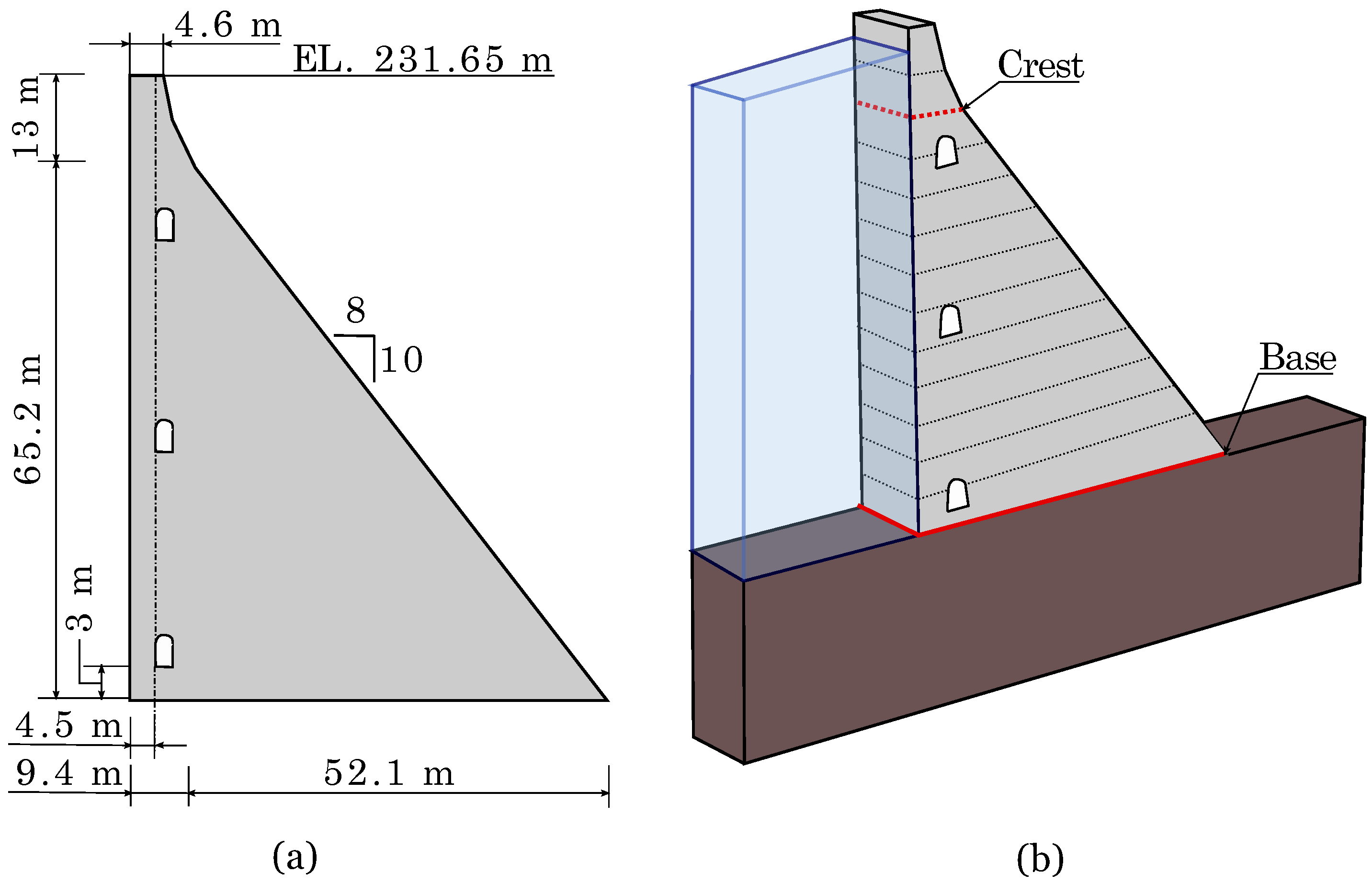
The present study is focused on a case study of a concrete gravity dam in Quebec, Canada. It is the largest gravity dam in the province, with 19 unkeyed monoliths, a maximum crest height of 78 m, and a crest length of 300 m (Figure 3a). The tallest monolith of the dam, with lift joints of 6 m, is selected as representative and modeled with the computer software CADAM3D [41] (Figure 3b), which performs stability analysis on gravity dams using the gravity method in accordance with the Canadian state-of-practice [9,11]. The validation of the numerical model was based on the fundamental period of the system and on global damping. By modifying the properties of the dam and of the foundation materials, the fundamental period and total damping of the system were and 1.05% respectively, which matches the results from in situ forced vibration tests [42]. Additionally, to perform all the simulations required for a probabilistic analysis, a script is created with MATLAB to automate the model runs. Only one loading case was analyzed; this case includes the self-weight of the block, the hydrostatic load exerted by the reservoir on the block, the uplift pressures at the concrete-foundation contact and the ice load per unit length. The uplift pressure distribution is defined according to the United States Army Corps of Engineers (USACE) [11]. A nonlinear analysis that allows to consider the crack propagation along the lift joints is used to analyze the system response, where if the base crack extends beyond the drain, the full uplift pressure is considered in the crack.
4.2. Performance Indicators
The overall stability of concrete retaining structures is verified by imposing performance criteria on predefined indicators to ensure that a sufficient margin of safety against failure exists for each of the failure mechanisms considered for the body of the system. The performance indicators used herein are (i) the sliding safety factor (SFF), (ii) the overturning safety factor (OSF), and (iii) the uplift safety factor (USF) and the position of the resulting force (PR). Table 1 shows the stability criteria for concrete gravity structures according to the Federal Energy Regulatory Commission (FERC) [43] and Canadian Dam Association (CDA) [9] guidelines. These guidelines propose SFs considering the level of knowledge in the strength parameters, where the required SFs are larger if no material tests are available. The LCs fall into three broad categories: normal, unusual, and extreme. These categories are related to a probability of exceedance for a period of time and at an acceptable level of safety. In the context of this study, only the conditions associated with water levels and ice loads are considered: normal operating conditions, unusual ice, or blocked drains and extreme safety floods.
4.3. Modeling Parameters and Screening Study
Each parameter in the analysis is defined either as a fixed value or as a RV. associated with a PDF. The preliminary set of considered parameters are selected taking into account the input parameters in the CADAM3D numerical model and the RVs considered in probabilistic analysis in the literature [15,19,22]. Table 2 presents the parameters that are considered as RVs in the numerical analysis of the dam response and for which the uncertainty or likelihood of occurrence is formally included. All the remaining input parameters are held constant and represented by their best estimate values. The probability distributions are defined using historical data from the case study dam and, when not available, empirical data from similar dams [8,44,45]. Based on literature results [46] and the dam owner’s expert judgement, it is assumed for the sampling and posterior analysis that 65% of the time, the concrete-rock contact is not bonded (apparent cohesion), while the remaining 35% of time, a special treatment is present that ensures the bond (real cohesion). In the same manner, it is considered that the lift joints (concrete-concrete contact) are always bonded. Note that Table 2 shows that some of the model parameters are correlated with and/or conditional on each other provided that the aforementioned assumptions are made. For the bonded case, the base peak cohesion is taken as twice the base tensile strength, BCP BRT, according to the Griffith criterion [47], while the base minimum peak compressive stress is null; hence, BMCP . Conversely, for the unbounded case, the base tensile strength is null, i.e., BRT, and the BMCP is normally distributed. Similarly, given that the base residual internal friction angle is always lower than or equal to the base peak friction angle, this parameter is considered equal to the peak friction angle minus a variation normally distributed. A uniform distribution is used for most of the parameters other than the minimum peak compressive stress so that more general cases can be considered in the analysis, as explained in the following sections.
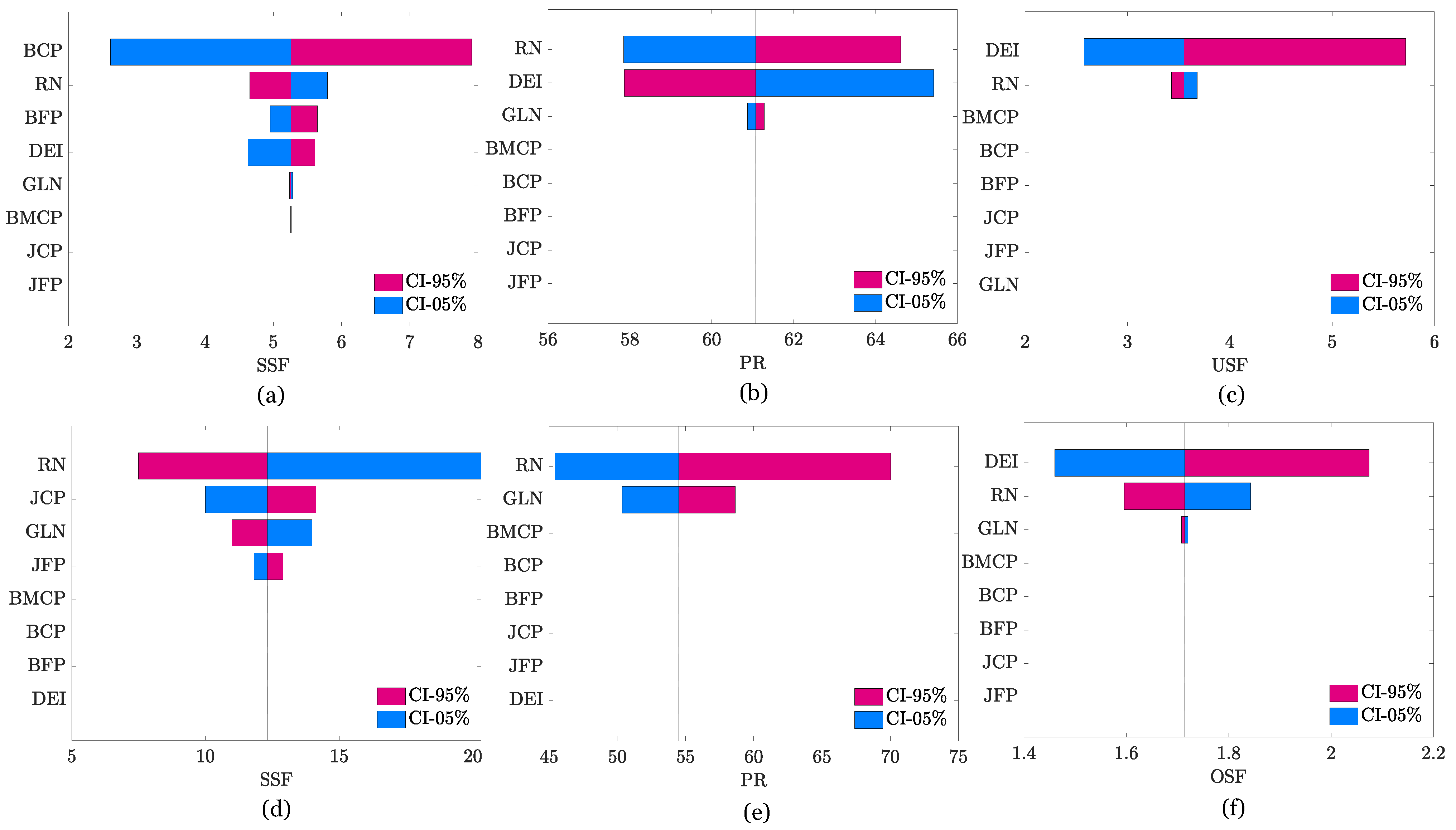
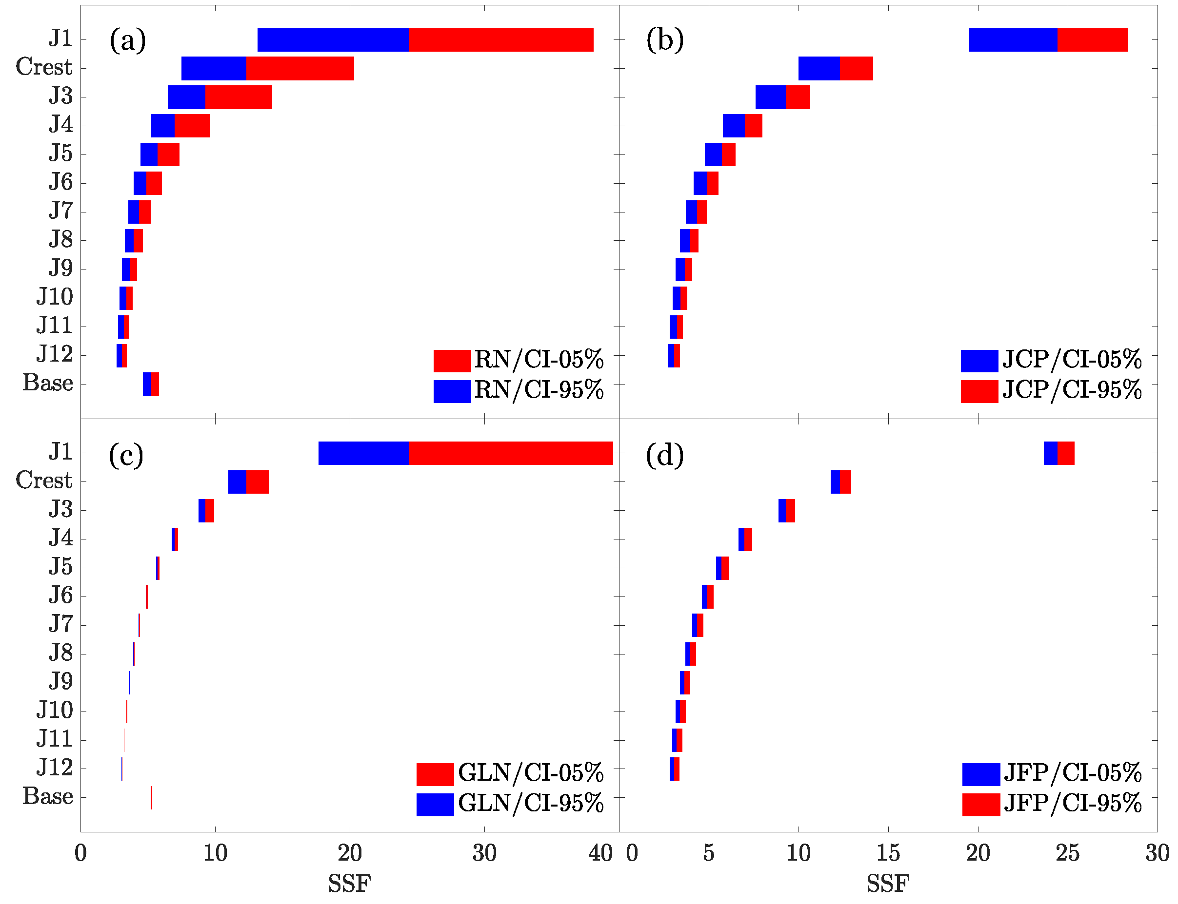
A screening study based on the TDs to assess the effect of each modeling parameter on the response of the dam is displayed in Figure 4. The reservoir elevation (RN), drain efficiency (DEI), and ice load (GLN) are some of the most influential parameters common to almost every performance indicator. However, note that the parameters most affecting a given response vary with respect to the considered lift joint, as shown in Figure 4a–d and Figure 4b,c. For this reason, Figure 5 presents the variation in the SSF with respect to loading and material property parameters for each joint. The effects of the joint peak cohesion (JCP) and RN are more significant for the upper lift joints and, as expected, this is even more evident for the GLN, whereas the joint peak friction angle (JFP) remains almost constant.
4.4. Load Combinations
In the structural safety evaluation of dams, unusual and extreme loads need particular attention, as there is more uncertainty because of low event accuracy. The evaluation has to consider two aspects: (i) load uncertainty and (ii) event frequency [15]. Table 3 displays the event frequency associated with each LC according to the dam owners’ internal regulations and based on the USACE guidelines [48].
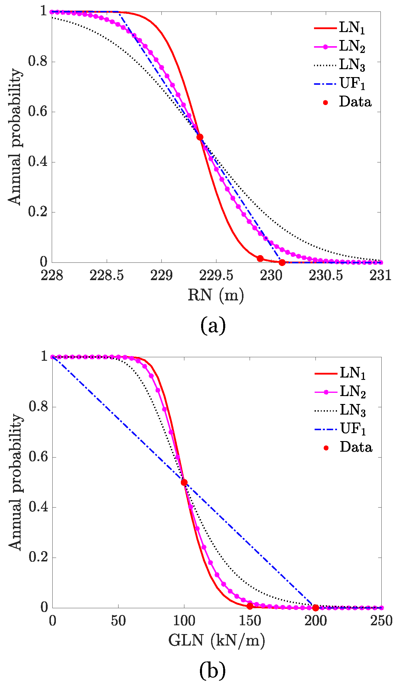
Taking into account the ice and reservoir load, Figure 6 presents the cumulative density function (CDF) associated with each load for determining the annual probability of exceedance. The red data dots are obtained based on the monitored reservoir values of the case study dam and the ice load traditionally used for each LC. To these points, a log-normal distribution is fitted in each case (LN). However, to better consider the load uncertainty and given that we are fitting a CDF with only 3 points, two other log-normal distributions are considered by keeping the same mean but doubling the standard deviation and using a uniform distribution with the same mean and an upper bound equal to the extreme condition. Table 4 provides the parameters of these distributions.
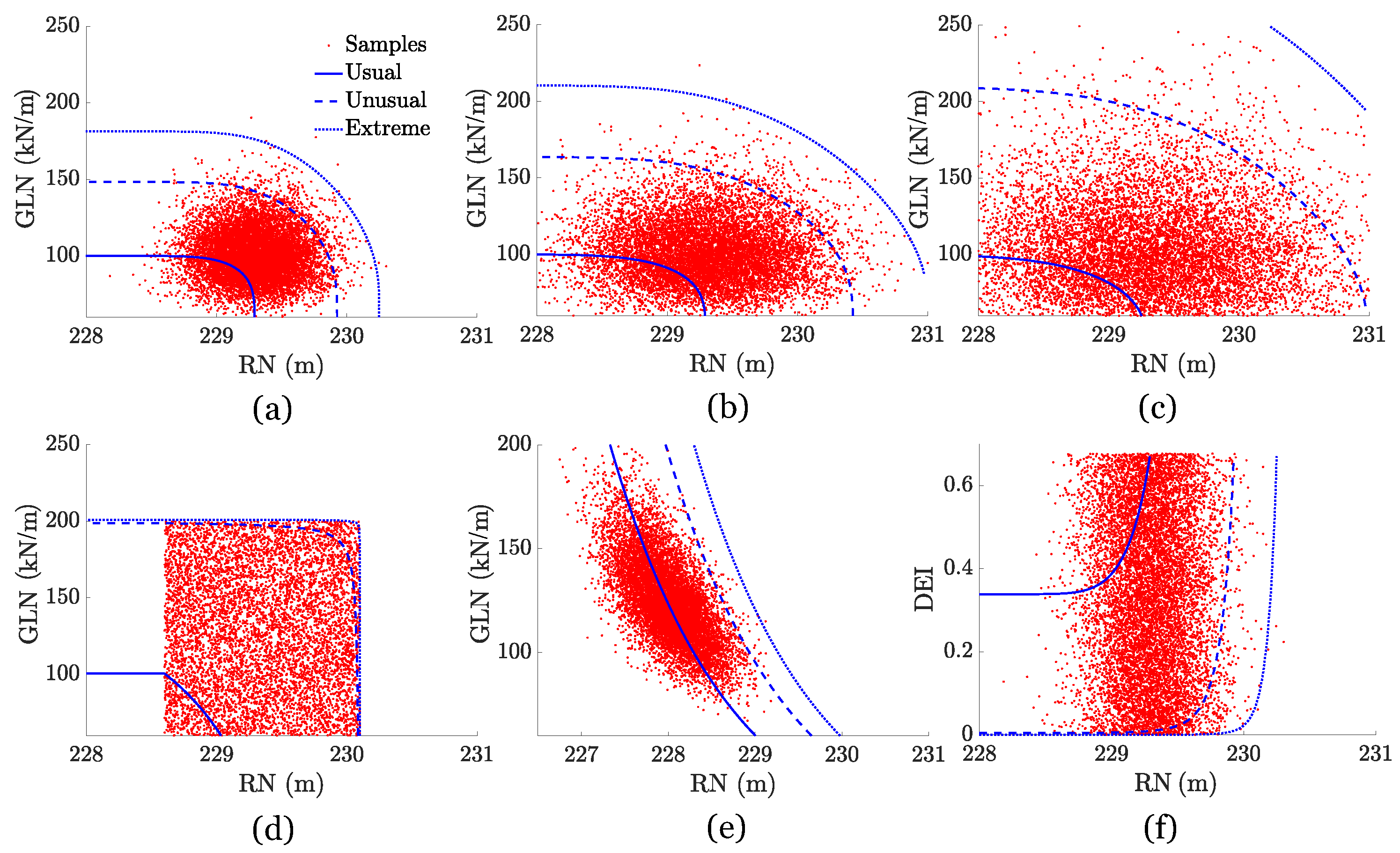
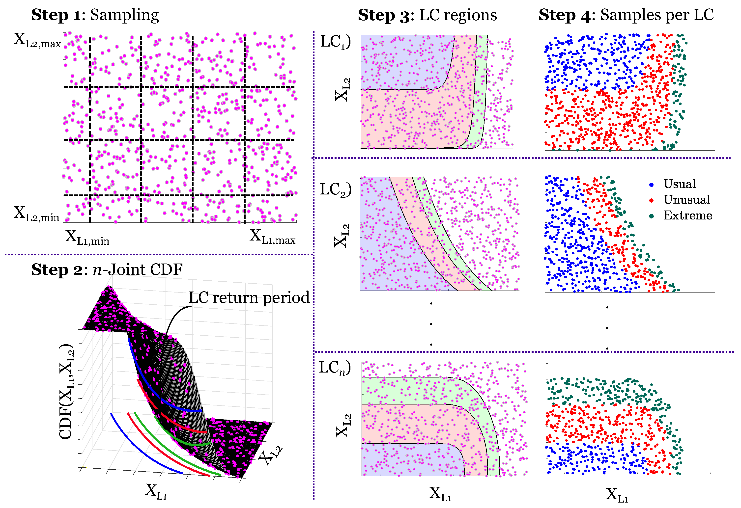
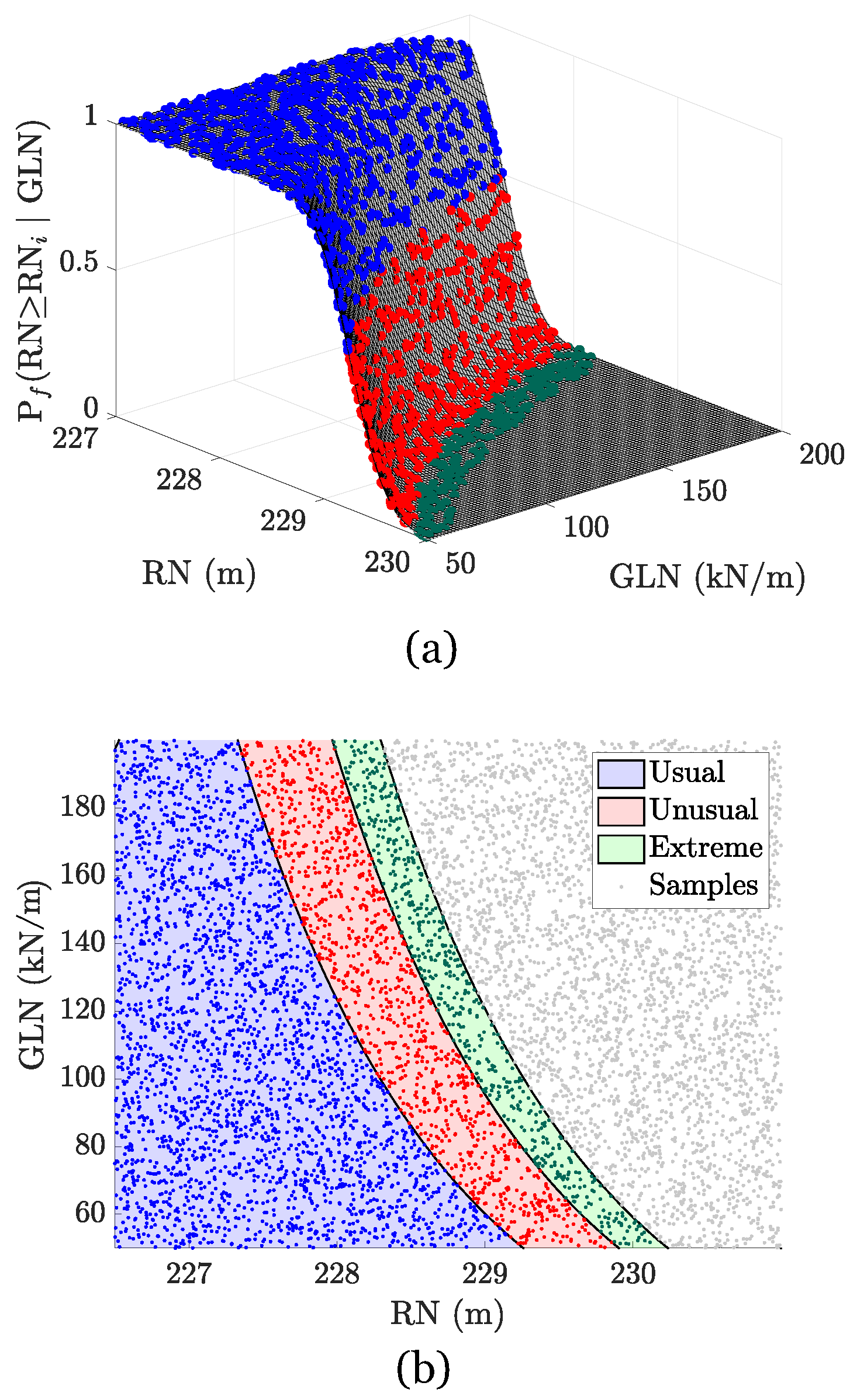
Figure 6a,b are combined to define the LCs by generating joint cumulative distribution functions, as shown in Table 5. Then, the joint cumulative distributions are intersected with horizontal constant probability planes equal to the annual probabilities defined in Table 3. Finally, the intersection is projected onto the XY plane and the regions corresponding to the usual, unusual, and extreme LCs are established, as shown in Figure 7. Figure 7a–d present these regions considering the independence between RN and GLN, whereas Figure 7e considers a negative correlation between RN and GLN, which provides a more realistic view of the case study dam’s reservoir management. In the same manner, given that, for some performance indicators, DEI is more critical than GLN (Figure 4b,c,f), Figure 7f defines the LC regions as a function of RN and DEI. Likewise, the samples displayed in Figure 7 are obtained with an LHS strategy considering that the samples are drawn from the target distributions defined in Table 5, which are the same distributions as those used for defining the LC regions. Notably, the samples are not evenly distributed in the LC regions, which implies that there is not a sufficient number of samples for the probabilistic analysis for each LC. To address these two main drawbacks, i.e., to upgrade the LC definitions and/or different LCs for different performance indicators and a more regular sampling space without the re-evaluation of the simulations, the methodology proposed in Figure 8 is used. First, PLHS is used to generate samples to be simulated with the numerical model considering only the upper and lower bounds of the possible range of values of the parameters defining the LC. Then, in Step 2, the joint CDF is built considering the distributions assigned to each of these parameters, and the joint cumulative probability is calculated for the samples drawn in Step 1 to ensure that they follow the target distributions. Next, in Step 3, the LC regions are defined by projecting on the XY plane the intersection curve of the joint CDF with horizontal planes corresponding to the annual probability of exceedance (Table 3). Finally, in Step 4, only the samples in Step 1 that fall in each LC region, i.e., the samples in which joint cumulative probability correspond to the prescribed annual probabilities of exceedance, are considered for the post-processing stage. Figure 9 presents the final samples per load combination for D5.
5. Results and Discussion
5.1. Sample Size
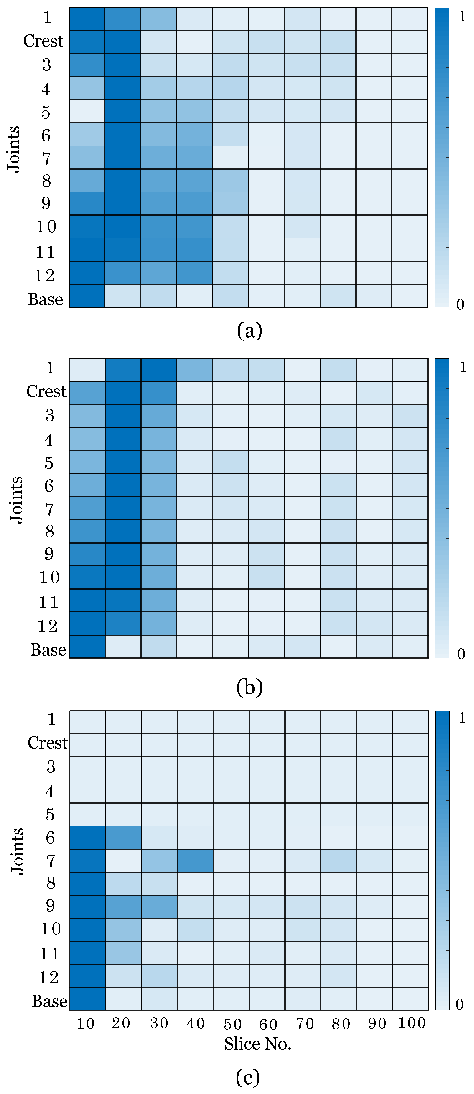
In the context of this study, and as a trade-off between the available computational budget and time, a maximum number of simulations is established. The total number of permitted simulations is divided into 100 slices, containing 100 samples each. The PLHS technique [38] is implemented via the VARS-Tool software package [49], which is a MATLAB Toolbox. Figure 10 presents the results of Equations (1)–(3) for each slice and for each joint. As seen from Figure 10, to obtain and within the specified tolerance, 50 slices are required, while, for , n = 60 are necessary. Even though the number of slices can be automatically determined by the algorithm, in this study, the number of slices is set to n = 55 given that with n = 50 the stopping condition in Equations (2) and (3) is already met. Ultimately, samples are considered for the probabilistic analysis.
5.2. Effect of Model Demand PDF Variation in the Analysis
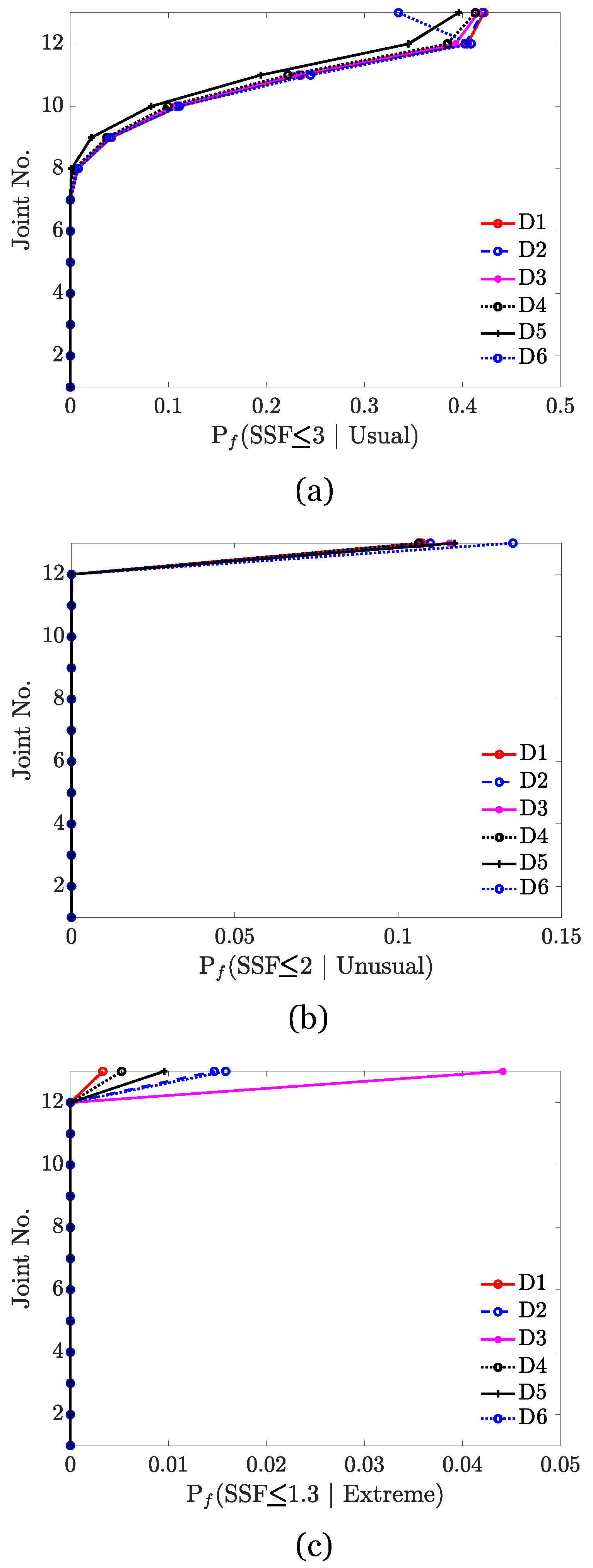
To assess the effect of the model demand parameter definition in the probabilistic analysis, the probability of exceeding a target SF conditioned on the LC is estimated. This probability is calculated according to Equation (4) considering the load combination distributions presented in Table 5. Figure 11 displays the probability of exceeding an SSF prescribed by the CDA guidelines (Table 1) given an usual, unusual, and extreme LCs for each lift joint. Note that, for the usual LC, the last 5 bottom lift joints are affected, while, for the unusual and extreme LCs, only the concrete-rock (base) joint is affected. This can be explained considering the SSF associated to the load case. Given that the concrete-concrete joints in general presented , for a less critical load case, i.e., a higher target safety factor, the probability of presenting a safety factor lower than the threshold for the usual load case is higher, thus affecting more joints. For the unusual and extreme LCs, the probability is even lower due to the considered target SSF, and only the base joint which present different material properties than the concrete-concrete joints is affected. It can be concluded that, for unusual and extreme load cases, only the base joint is critical, while, for usual loading conditions, attention must be also paid to the last 5 bottom joints. Moreover, it is observed that using distributions that more realistically represent the LCs, such as D5, which considers that during the summer, the reservoir is high, and the ice load is low, and vice versa, provide less conservative probabilities of exceedance. Only the functions corresponding to the sliding stability criteria are presented given that the numerical model simulations showed that OSF and USF are always respected, highlighting the adequate performance of the case-study dam.
5.3. Model Parameter Recommendations for Adequate Performance
5.3.1. Influence of Model Parameters
The significance of each modeling parameter in Table 2 on the structural response of the dam is also assessed by a screening study using ANOVA. For each response monitored, a multiway ANOVA is conducted using MATLAB. The results of this analysis are shown in Table 6, where the p-values < 0.05 indicate statistically significant parameters that should be treated with special attention. It should be mentioned that, for a pure sensitivity analysis, as is the case here, using uniform distributions is acceptable, but not for a reliability analysis since it is hard to find a physical parameter (e.g., the rock/concrete strength parameters) that follows a uniform distribution. The results are presented for the base and crest lift joints, which are considered as representative of the system.
Overall, the results reveal that all the parameters have a statistically significant effect on at least one of the critical dam responses. Additionally, the parameters used to define the LCs, such as RN, GLN, and DEI, are important for every SF at the base and/or the crest. These results can be used to reduce the number of parameters considered in the probabilistic analysis; however, given that nearly all the parameters are identified as significant for at least one of the response quantities of interest, this approach is not used. Beyond this, however, the results of the screening study are useful for better understanding the effect of the joint parameter variations on the dam’s response and to validate the results of more simplified methods, such as the TD.
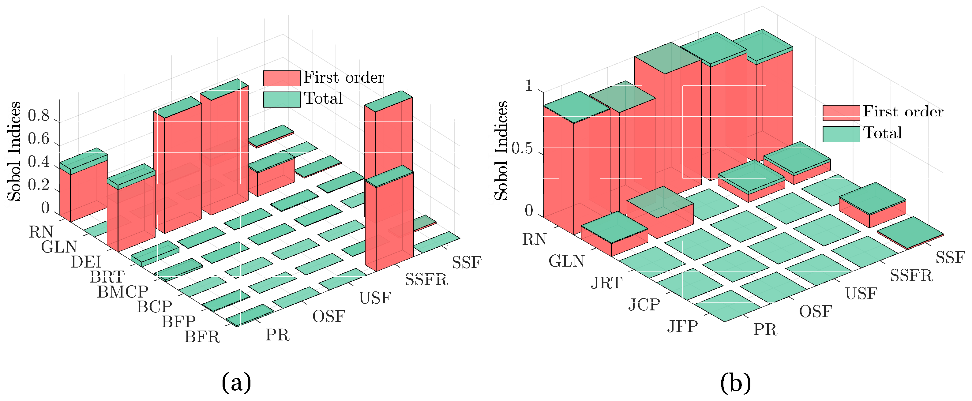
In the same way as for the multiway ANOVA, for each response monitored, Sobol’s indices were calculated using UQLab [50] through MATLAB. Total sensitivity indices, which measure the main effects of a given parameter and all the interactions (of any order) involving that parameter, as well as the first order indices (no interaction), were estimated as shown in Figure 12. It is observed from Figure 12a that, for the concrete-rock joint, the parameters which had the greatest effect on the monitored response are RN, DEI, BFP, and BFR. Particularly, the most important parameters for PR are RN and DEI, DEI and BFR for SSFR, BCP for SSF, and DEI for OSF and USF. On the contrary, it is observed from Figure 12b that, for the concrete-concrete joint, the most important parameter is RN, followed by GLN and JCP. In general, the parameters affecting the most PR, OSF, and SSFR are RN and GLN, while RN, GLN, and JCP have the most influence on SSF. Finally, only RN affects USF.
5.3.2. Stability Analysis Results
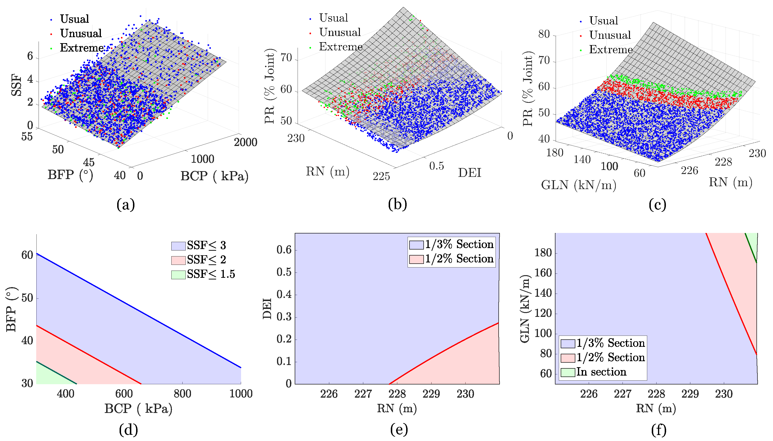
The final system output, together with the global sensitivity analysis, can also be used to assess the dam performance through the formulation of safety recommendations. To this end, the simulation results for the base SSF and PR at the base and at the crest are plotted against the two most influential parameters according to Figure 4 and Figure 12. The simulation results are presented in Figure 13a–c, where it can be seen that the response of interest can be approximated well by a surface defined with only two model parameters, as shown in Table 7.
Finally, ranges of values that meet the SFs provided by safety guidelines are formulated by intersecting the parametric surfaces with horizontal planes at the target SFs specified in Table 1. Figure 13d presents the BCP-BFP zones that result in base SSF values lower than those prescribed by the CDA [9], while Figure 13e,f present the RN-DEI and RN-GLN zones that provide a resultant within the and median of the base for the base and the crest lift joints, respectively.
6. Conclusions
Uncertainties prevail in the safety assessment of dams, particularly in the identification of failure modes, loading conditions and model parameter estimations. Hence, it is important to consider various sources of uncertainties for the safety assessment of dams, and the means to do so is through a probabilistic analysis. The main goal of this study was to develop a probabilistic-based methodology to sufficiently assess the safety of dams with a flexible sampling strategy so that new data can be easily and efficiently incorporated in the analysis without the re-evaluation of the system simulations. Moreover, a prescreening of the model parameter sensitivity was performed with the generation of TDs, which was later validated with variance-based global sensitivity analysis methods, such as ANOVA and Sobol’s indices. Finally, safety recommendations were formulated by evaluating the system output, and the probability of the target SF exceeding the guidelines given a determined LC was estimated.
The proposed procedure is more robust, computationally efficient, and more easily interpretable than conventional methods while accounting for uncertainties in the resistance and loading parameters, which would otherwise be neglected. The perspective taken is that dam safety assessment is a tool for providing insights that can strengthen both the engineering and decision aspects of dam safety management. As such, this study will allow professionals in the dam industry and dam owners to expedite the safety assessment of gravity dams and to identify the parameter uncertainties affecting the dam response the most so that economic resources can be invested in the exhaustive study of these parameters.
Author Contributions
Conceptualization, R.L.S. and B.M.; methodology, R.L.S.; validation, B.M., P.P. and Jamie E. Padgett; formal analysis, R.L.S.; resources, P.P. and B.M.; writing—original draft preparation, R.L.S.; writing—review and editing, P.P.; visualization, J.E.P.; supervision, P.P. and B.M.; project administration, P.P.; funding acquisition, P.P. All authors have read and agreed to the published version of the manuscript.
Funding
The authors acknowledge the financial support of MITACS, the Natural Sciences and Engineering Research Council of Canada (NSERC) and the Fonds de recherche du Quebec–Nature et technologies (FRQNT).
Institutional Review Board Statement
Not applicable.
Informed Consent Statement
Not applicable.
Data Availability Statement
The data presented in this study are available on request from the corresponding author. The data are not publicly available due to privacy.
Acknowledgments
The authors acknowledge the financial support of MITACS, the Natural Sciences and Engineering Research Council of Canada (NSERC) and the Fonds de recherche du Quebec – Nature et technologies (FRQNT). Any opinions, findings, and conclusions or recommendations expressed in this paper are those of the authors and do not necessarily reflect the views of the sponsors.
Conflicts of Interest
The authors declare no conflict of interest. The funders had no role in the design of the study; in the collection, analyses, or interpretation of data; in the writing of the manuscript, or in the decision to publish the results.
References
- Li, Z. Global Sensitivity Analysis of the Static Performance of Concrete Gravity Dam from the Viewpoint of Structural Health Monitoring. Arch. Comput. Methods Eng. 2020. [Google Scholar] [CrossRef]
- Cordier, M.; Léger, P. Structural stability of gravity dams: A progressive assessment considering uncertainties in shear strength parameters. Georisk Assess. Manag. Risk Eng. Syst. Geohazards 2018, 12, 109–122. [Google Scholar] [CrossRef]
- Westberg Wilde, M.; Johansson, F. Probability-based guidelines for design and assessment of concrete dams. In Safety, Reliability, Risk and Life-Cycle Performance of Structures & Infrastructures; Deodatis, E.F., Ed.; Taylor & Francis Group: London, UK, 2013; pp. 5187–5210. [Google Scholar]
- Kalinina, A.; Spada, M.; Marelli, S.; Burgherr, P.; Sudret, B. Uncertainties in the Risk Assessment of Hydropower Dams: State-of-the-Art and Outlook; Rapport Technique RSUQ-2016-008; ETH Zurich: Zürich, Switzerland, 2016. [Google Scholar]
- Segura, R.; Padgett, J.; Paultre, P. Metamodel-Based Seismic Fragility Analysis of Concrete Gravity Dams. J. Struct. Eng. 2020, 46, 04020121. [Google Scholar] [CrossRef] [Green Version]
- Hariri-Ardebili, M.; Pourkamali-Anaraki, F. Simplified reliability analysis of multi hazard risk in gravity dams via machine learning techniques. Arch. Civ. Mech. Eng. 2018, 18, 592–610. [Google Scholar] [CrossRef]
- Salazar, F.; Morán, R.; Toledo, M.Á.; Oñate, E. Data-based models for the prediction of dam behaviour: A review and some methodogical considerations. Arch. Comput. Methods Eng. 2015, 24, 1–21. [Google Scholar] [CrossRef] [Green Version]
- Schleiss, A.; Pougatsch, H. Les Barrages, du Project a la Mise en Service, 1st ed.; Presses Polytechniques et Universitaires Romandes: Lausanne, Switzerland, 2011. [Google Scholar]
- CDA. Dam safety Guidelines. In Dam Safety Recommendations Section 6.1, 6.2 and 6.3, Revised in 2013; Canadian Dam Association: Winnipeg, MB, Canada, 2007. [Google Scholar]
- FERC. Engineering Guidelines for the Evaluation of Hydropower Projects; Federal Energy Regulatory Comission: Washington, DC, USA, 2002.
- USACE. Gravity Dam Design; Technical Report EM 1110-2-2200; U.S. Corps of Engineer: Washington, DC, USA, 1995.
- Lave, L.B.; Resendiz-Carrillo, D.; McMichael, F.C. Safety goals for high-hazard dams: Are dams too safe? Water Resour. Res. 1990, 26, 1383–1391. [Google Scholar]
- Tekie, P.; Ellingwood, B. Seismic fragility assessment of concrete gravity dams. Earthq. Eng. Struct. Dyn. 2003, 32, 2221–2240. [Google Scholar] [CrossRef]
- Schultz, M.; Gouldby, B.; Simm, J.; Wibowo, J. Beyond the Factor of Safety: Developing Fragility Curves to Characterize System Reliability; Technical Report ERDC SR-10-01; U.S. Army Corps of Engineers: Washington, DC, USA, 2010.
- Kreuzer, H.; Léger, P. The Adjustable Factor of Safety: A reliability-based approach to assess the factor of safety for concrete dams. Int. J. Hydropower Dams 2013, 20, 67–80. [Google Scholar]
- Westberg Wilde, M.; Johansson, F. System reliability of concrete dams with respect to foundation stability: Application to a spillway. J. Geotech. Geoenviron. Eng. 2013, 139, 308–319. [Google Scholar] [CrossRef]
- Bernier, C.; Padgett, J.; Proulx, J.; Paultre, P. Seismic fragility of concrete gravity dams with modeling parameter uncertainty and spacial variation. J. Struct. Eng. 2016, 142, 05015002. [Google Scholar] [CrossRef]
- Hariri-Ardebili, M. Analytical failure probability model for generic gravity dam classes. Proc. Inst. Mech. Eng. J. Risk Reliab. 2017, 1–12. [Google Scholar] [CrossRef]
- Segura, R.; Bernier, C.; Durand, C.; Paultre, P. Modelling and Characterizing a Concrete Gravity Dam for Fragility Analysis. Infrastructures 2019, 4, 1–19. [Google Scholar]
- USBR and USACE. Best Practices in Dam and Levee Safety Risk Analysis; Technical Report Version 4.1; U.S. Bureau of Reclammation: Washington, DC, USA; U.S. Army Corps of Engineer: Washington, DC, USA, 2019.
- Hovde, E. Recommendations for Existing Concrete Dams: Probabilistic Analysis of Stability; Rapport Technique 12372-OO-R-001; Dr.techn.Olav Olsen AS: Trondheim, Norway, 2017. [Google Scholar]
- Westberg, M.; Johansson, F. Probabilistic Model Code for Concrete Dams; Rapport Technique 2016:292; Energiforsk: Stockholm, Sweden, 2016. [Google Scholar]
- FERC. Risk-Informed Decision Making Guidelines; Version 4.1; Federal Energy Regulatory Comission: Washington, DC, USA, 2016.
- FEMA. Federal Guidelines for Dam Safety Risk Management; Technical Report P-1025. Federal Guidelines for Dam Safety Risk Management; Federal Emergency Management Agency (FEMA): Washington, DC, USA, 2015.
- Escuder-Bueno, I.; Mazza, G.; Morales-Torres, A.; Castillo-Rodriguez, J.T. Computational Aspects of Dam Risk Analysis: Findings and Challenges. Engineering 2016, 2, 319–324. [Google Scholar] [CrossRef] [Green Version]
- Krounis, A.; Johansson, F.; Larsson, S. Effects of spatial variation in cohesion over the concrete-rock interface on dam sliding stability. J. Rock Mech. Geotech. Eng. 2015, 7, 659–667. [Google Scholar] [CrossRef] [Green Version]
- Altarejos-Garcia, L.; Escuder-Bueno, I.; Serrano-Lombillo, A.; Morales-Torres, A. Factor of safety and probability of failure in concrete dams. In Risk Analysis, Dam Safety, Dam Security and Critical Infrastructure Management; CRC Press: Boca Raton, FL, USA, 2012. [Google Scholar]
- USBR. Dam Safety Public Protection Guidelines: A Risk Framework to Support Dam Safety Decision-Making; Technical Report August; U.S. Bureau of Reclammation: Washington, DC, USA, 2011.
- Howard, R.A. Decision analysis: Practice and promise. Manag. Sci. 1988, 34, 679–695. [Google Scholar] [CrossRef] [Green Version]
- Porter, K. An overview of PEER’s performance-based earthquake engineering methodology. In Proceedings of the 9th International Conference on Applications of Statistics and Probability in Civil Engineering, San Francisco, CA, USA, 6–9 July 2003. [Google Scholar]
- Hariri-Ardebili, M.A.; Saouma, V. Sensitivity and uncertainty quantification of the cohesive crack model. Eng. Fract. Mech. 2016, 155, 18–35. [Google Scholar] [CrossRef]
- Hariri-Ardebili, M. MCS-based response surface metamodels and optimal design of experiments for gravity dams. Struct. Infraestruct. Eng. 2018. [Google Scholar] [CrossRef]
- Lokke, A.; Chopra, A.K. Direct-Finite-Element Method for Nonlinear Earthquake Analysis of Concrete Dams Including Dam-Water-Foundation Rock Interaction; Technical Report 2019/02; Pacific Earthquake Engineering Research Center: Richmond, CA, USA, 2019. [Google Scholar]
- Sobol, I. Global sensitivity indices for nonlinear mathematical models and their monte carlo estimates mathematics and computers in simulations. Math. Comput. Simul. 2001, 55, 271–280. [Google Scholar] [CrossRef]
- Gaspar, A.; Lopez-Caballero, F.; Modaressi-Farahmand-Razavi, A.; Gomes-Correia, A. Methodology for a probabilistic analysis of an RCC gravity dam construction. Modelling of temperature, hydration degree and ageing degree fields. Eng. Struct. 2014, 65, 99–110. [Google Scholar] [CrossRef]
- Khaneghahi, M.H.; Alembagheri, M.; Soltani, N. Reliability and variance-based sensitivity analysis of arch dams during construction and reservoir impoundment. Front. Struct. Civ. Eng. 2018, 13, 526–541. [Google Scholar] [CrossRef]
- Zhang, L.; Peng, M.; Chang, D.; Xu, Y. Dam Failure Mechanism and Risk Assessment; Wiley: Singapore, 2016. [Google Scholar]
- Sheikholeslami, R.; Razavi, S. Progressive Latin Hypercube Sampling: An efficient approach for robust sampling-based analysis of environmental models. Environ. Model. Softw. 2017, 93, 109–126. [Google Scholar] [CrossRef]
- Saltelli, A.; Tarantola, S.; Campolongo, F.; Ratto, M. Sensitivity Analysis in Practice: A Guide to Assessing Scientific Models; Wiley: Ispra, Italy, 2004. [Google Scholar]
- Padgett, J.; DesRoches, R. Sensitivity of Seismic Response and Fragility to Parameter Uncertainty. J. Struct. Eng. 2007, 133, 1710–1718. [Google Scholar] [CrossRef] [Green Version]
- CADAM3D; Version 2.4; Mlt Technology Inc.: Westport, IN, USA, 2020.
- Proulx, J.; Paultre, P. Experimental and numerical investigation of dam-reservoir-foundation interaction for a large gravity dam. Can. J. Civ. Eng. 1997, 24, 90–105. [Google Scholar]
- FERC. Engineering Guidelines for the Evaluation of Hydropower Projects: Chapter 3, Gravity Dams; Revised Version; Federal Energy Regulatory Comission: Washington, DC, USA, 2016.
- Rivard, P.; Champagne, K.; Quirion, M. Paramètres de résistance au cisaillement associés aux discontinuités des barrages en béton du Québec. In Proceedings of the Annual Congress of the Canadian Dam Association, Montreal, QC, Canada, 5–10 October 2013. [Google Scholar]
- Ruggeri, G. Working Group on Sliding Safety of Existing Gravity Dams; Technical Report; ICOLD European Club: Paris, France, 2004. [Google Scholar]
- Renaud, S.; Saichi, T.; Bouaanani, N.; Miquel, B.; Quirion, M.; Rivard, P. Roughness Effects on the Shear Strength of Concrete and Rock Joints in Dams Based on Experimental Data. Rock Mech. Rock Eng. 2019, 52, 3867–3888. [Google Scholar] [CrossRef]
- Griffith, A. The phenomena of rupture and flow in solids. Philos. Trans. R. Soc. Lond 1921, 221, 163–198. [Google Scholar]
- USACE. Introduction to Probability and Reliability Methods for Use in Geotechnical Engineering; U.S. Army Corps of Engineers: Washington, DC, USA, 1997.
- Razavi, S.; Sheikholeslami, R.; Gupta, H.V.; Haghnegahdar, A. VARS-TOOL: A toolbox for comprehensive, efficient, and robust sensitivity and uncertainty analysis. Environ. Model. Softw. 2018, 112, 95–107. [Google Scholar] [CrossRef]
- Marelli, S.; Sudret, B. UQLab: A Framework for Uncertainty Quantification in MATLAB. In Proceedings of the 2nd International Conference on Vulnerability and Risk Analysis and Management (ICVRAM 2014), Liverpool, UK, 13–16 July 2014; pp. 2554–2563. [Google Scholar]
Figure 1.
Probabilistic-based procedure.

Figure 2.
Tornado diagram (TD) methodology.

Figure 3.
Case study dam: (a) cross-section and (b) CADAM3D numerical model of the tallest monolith.
Figure 3.
Case study dam: (a) cross-section and (b) CADAM3D numerical model of the tallest monolith.

Figure 4.
TD: (a) Base joint—sliding safety factor (SSF), (b) Base joint—position of the resulting force (PR), (c) Base joint—uplift safety factor (USF), (d) Crest joint—SSF, (e) Crest joint—PR, and (f) Base joint—overturning safety factor (OSF).
Figure 4.
TD: (a) Base joint—sliding safety factor (SSF), (b) Base joint—position of the resulting force (PR), (c) Base joint—uplift safety factor (USF), (d) Crest joint—SSF, (e) Crest joint—PR, and (f) Base joint—overturning safety factor (OSF).

Figure 5.
Joint TD for the SSF: (a) reservoir elevation (RN), (b) joint peak cohesion (JCP), (c) ice load (GLN), and (d) peak friction angle (JFP).
Figure 5.
Joint TD for the SSF: (a) reservoir elevation (RN), (b) joint peak cohesion (JCP), (c) ice load (GLN), and (d) peak friction angle (JFP).

Figure 6.
Annual probability of exceedance: (a) RN and (b) GLN.

Figure 7.
LC regions for RN-GLN: (a) D1, (b) D2, (c) D3, (d) D4, (e) D5, and (f) D6.

Figure 8.
Procedure for obtaining samples per LC.

Figure 9.
Samples per LC for D5: (a) cumulative density function, and (b) XY projection.

Figure 10.
Progressive Latin hypercube sampling (PLHS) slice iterations: (a) , (b) , and (c) .

Figure 11.
Conditional probability functions: (a) usual, (b) unusual, and (c) extreme.

Figure 12.
Sobol indices: (a) Base and (b) Crest.

Figure 13.
Stability analysis output: (a) SSF-Base, (b) PR-Base, (c) PR-Crest, (d) BCP-BFP regions, (e) RN-drain efficiency (DEI) regions and (f) RN-GLN regions.
Figure 13.
Stability analysis output: (a) SSF-Base, (b) PR-Base, (c) PR-Crest, (d) BCP-BFP regions, (e) RN-drain efficiency (DEI) regions and (f) RN-GLN regions.


Table 1.
Stability criteria.
| LC | SSF | OSF | USF | PR | ||
|---|---|---|---|---|---|---|
| No Test | Test | Residual | ||||
| Usual | 3 | 2 | 1.5 | 1.2 | 1/3 median | |
| Unusual | 2 | 1.5 | 1.3 | 1.1 | 1/2 median | |
| Extreme | 1.3 | 1.1 | 1.1 | 1.1 | within base | |
† Friction and cohesion, ‡ Friction only.
Table 2.
Uncertain parameters.
| Parameter | Designation | Distribution Parameters | ||
|---|---|---|---|---|
| Reservoir elevation (m) | RN | Uniform | L = 225 | U = 231 |
| Ice load (kN/m) | GLN | Uniform | L = 50 | U = 200 |
| Drain efficiency (%) | DEI | Uniform | L = 0 | U = 67 |
| Base peak friction angle () | BFP | Uniform | L = 42 | U = 55 |
| Base residual friction angle () | BFR | Normal | BFP | |
| Base tensile strength (kPa) | BRT | Uniform | L = 150 | U = 1500 |
| Base min. peak compressive stress (kPa) | BMCP | Normal | ||
| Base peak cohesion - Real (kPa) | BCP | Uniform | L = 300 | U = 3000 |
| Base peak cohesion - Apparent (kPa) | BCP | Uniform | L = 0 | U = 1000 |
| Joint tensile strength (kPa) | JRT | Uniform | L = 1000 | U = 3000 |
| Joint peak friction angle () | JFP | Uniform | L = 45 | U = 55 |
| Joint peak cohesion (kPa) | JCP | Uniform | L = 400 | U = 700 |
The base parameters refer to the concrete-rock contact. The joint parameters refer to the concrete-concrete contact.
Table 3.
Probabilities associated with load combinations (LCs).
| Load Combination (LC) | Annual Probability (P) | Return Period (RP) |
|---|---|---|
| Usual | P | RP years |
| Unusual | P | RP years |
| Extreme | P | RP years |
Table 4.
Loading parameter distributions.
| CDF | Distribution Parameters | |||||
|---|---|---|---|---|---|---|
| RN | GLN | DEI | ||||
| LN | 5.34 | 0.001 | 4.60 | 0.10 | – | – |
| LN | 5.34 | 0.002 | 4.60 | 0.20 | – | – |
| LN | 5.34 | 0.003 | 4.60 | 0.30 | – | – |
| UF | L | U | L | U | L | U |
Table 5.
Considered LC distributions.
| LC Distribution | Parameter | Description |
|---|---|---|
| D1 | RN-GLN | LN LN |
| D2 | RN-GLN | LN LN |
| D3 | RN-GLN | LN LN |
| D4 | RN-GLN | UF UF |
| D5 | RN-GLN | LN LN with |
| D6 | RN-DEI | LN UF |
† Estimated from expert judgement and the historical reservoir management of the case study dam.
Table 6.
p-values from ANOVA: summarizing the significant parameters for the base and neck sliding of the dam.
Table 6.
p-values from ANOVA: summarizing the significant parameters for the base and neck sliding of the dam.
| Model Parameter | SSF | SSFR | USF | OSF | PR | |||||
|---|---|---|---|---|---|---|---|---|---|---|
| Base | Crest | Base | Crest | Base | Crest | Base | Crest | Base | Crest | |
| RN | <0.05 | <0.05 | <0.05 | <0.05 | <0.05 | <0.05 | <0.05 | <0.05 | <0.05 | <0.05 |
| GLN | <0.05 | <0.05 | <0.05 | <0.05 | 0.657 | 0.233 | 0.070 | <0.05 | <0.05 | <0.05 |
| DEI | <0.05 | – | <0.05 | – | <0.05 | – | <0.05 | – | <0.05 | – |
| BRT | <0.05 | – | 0.087 | – | 0.215 | – | 0.191 | – | 0.151 | – |
| BMCP | <0.05 | – | <0.05 | – | <0.05 | – | 0.104 | – | <0.05 | – |
| BCP | <0.05 | – | 0.167 | – | 0.615 | – | 0.538 | – | 0.428 | – |
| BFP | <0.05 | – | 0.913 | – | 0.970 | – | 0.915 | – | 0.444 | – |
| BRF | 0.532 | – | <0.05 | – | 0.917 | – | 0.964 | – | 0.339 | – |
| JRT | – | 0.206 | – | 0.096 | – | <0.05 | – | <0.05 | – | 0.060 |
| JCP | – | <0.05 | – | 0.093 | – | <0.05 | – | <0.05 | – | 0.060 |
| JPF | – | <0.05 | – | 0.251 | – | 0.190 | – | 0.231 | – | 0.315 |
† Friction and cohesion, ‡ Friction only.
Table 7.
Parametric surface goodness-of-fits.
| Surface | R | RMSE |
|---|---|---|
| SSF (BCP, BFP) | 0.963 | 0.3613 |
| PR (RN, DEI) | 0.901 | 1.450 |
| PR (RN, GLN) | 0.999 | 0.101 |
Publisher’s Note: MDPI stays neutral with regard to jurisdictional claims in published maps and institutional affiliations. |
© 2021 by the authors. Licensee MDPI, Basel, Switzerland. This article is an open access article distributed under the terms and conditions of the Creative Commons Attribution (CC BY) license (http://creativecommons.org/licenses/by/4.0/).
Share and Cite
MDPI and ACS Style
Segura, R.L.; Miquel, B.; Paultre, P.; Padgett, J.E. Accounting for Uncertainties in the Safety Assessment of Concrete Gravity Dams: A Probabilistic Approach with Sample Optimization. Water 2021, 13, 855. https://doi.org/10.3390/w13060855
AMA Style
Segura RL, Miquel B, Paultre P, Padgett JE. Accounting for Uncertainties in the Safety Assessment of Concrete Gravity Dams: A Probabilistic Approach with Sample Optimization. Water. 2021; 13(6):855. https://doi.org/10.3390/w13060855
Chicago/Turabian StyleSegura, Rocio L., Benjamin Miquel, Patrick Paultre, and Jamie E. Padgett. 2021. "Accounting for Uncertainties in the Safety Assessment of Concrete Gravity Dams: A Probabilistic Approach with Sample Optimization" Water 13, no. 6: 855. https://doi.org/10.3390/w13060855
Note that from the first issue of 2016, this journal uses article numbers instead of page numbers. See further details here.