
Regional Downscaling of Copernicus ERA5 Wave Data for Coastal Engineering Activities and Operational Coastal Services


Department of Engineering, Roma Tre University, 00161 Rome, Italy
*
Author to whom correspondence should be addressed.
Water 2021, 13(6), 859; https://doi.org/10.3390/w13060859
Submission received: 3 March 2021
/
Accepted: 19 March 2021
/
Published: 22 March 2021
(This article belongs to the Special Issue Coastal Sediment Management: From Theory to Practice)
Abstract
:Hindcasted wind and wave data, available on a coarse resolution global grid (Copernicus ERA5 dataset), are downscaled by means of the numerical model SWAN (simulating waves in the nearshore) to produce time series of wave conditions at a high resolution along the Italian coasts in the central Tyrrhenian Sea. In order to achieve the proper spatial resolution along the coast, the finite element version of the model is used. Wave data time series at the ERA5 grid are used to specify boundary conditions for the wave model at the offshore sides of the computational domain. The wind field is fed to the model to account for local wave generation. The modeled sea states are compared against the multiple wave records available in the area, in order to calibrate and validate the model. The model results are in quite good agreement with direct measurements, both in terms of wave climate and wave extremes. The results show that using the present modeling chain, it is possible to build a reliable nearshore wave parameters database with high space resolution. Such a database, once prepared for coastal areas, possibly at the national level, can be of high value for many engineering activities related to coastal area management, and can be useful to provide fundamental information for the development of operational coastal services.
Keywords:
waves; wind; Copernicus program; ERA5; SWAN model; nearshore; coastal zone; coastal erosion1. Introduction
The coastal areas are, worldwide, the most densely populated, and where many strategic, economic, and social interests are concentrated. They represent, on the one hand, a delicate environment, as anthropic activities might induce unacceptable damages to the environment and to the coastal landscapes. On the other hand, the marine environment is extremely aggressive, and natural catastrophes along the coast cause huge losses every year in terms of both human lives and economic goods.
The sustainable development and the management of the coastal areas can be fostered and supported by, among other things, engineering activities that should be carefully based on an in-depth knowledge of the environment. For example, in order to support knowledge-based management of sediments moving along the coast, it is crucial to properly describe the nearshore hydrodynamic phenomena that drive littoral transport, such as wave-breaking induced longshore currents. Among the many physical parameters of great importance when describing the coastal zone, a key role is therefore played by meteoceanographic factors, such as waves, winds, currents, and sea levels. In order to properly drive engineering activities, these should be known in terms of their average and extreme values.
Furthermore, as part of the Italian Copernicus User Forum and the Space Economy Mirror Copernicus activities, recent research [1] has defined the needs of Italian institutions and users involved in the management of coastal areas. Among other results, it has turned out that a careful knowledge of the meteoceanographic factors mentioned above is of the utmost importance for the proper development of their institutional activities. It is therefore desirable that operational coastal services, to be implemented at the national level as downstream products of Copernicus data and Core Services, will be able to provide, with accurate, high resolution, nearshore data of these physical quantities.
In general, the required information on the meteoceanographic factors can be obtained from direct measurements or by model hindcasts. Certainly, the direct measurements are of fundamental importance and represent the primary source of knowledge on the marine environment. Measurement devices are generally expensive, and their use is de facto feasible for few locations in space and with reference to limited time windows. Remote systems, both ground- and satellite-based, represent a modern and very promising alternative that can provide data at the global or regional scale with relatively low cost for large technical and scientific communities.
Model hindcasts are typically based on global re-analysis, carried out by applying meteorological models to the past, possibly with the assimilation of measurements. On the basis of the wind fields, third-generation ocean wave models, such as WAM [2,3,4], WAVEWATCH III [5,6,7], and SWAN (simulating waves in the nearshore) [8,9], are applied to reconstruct the sea states. Global hindcasts [10] can then be used to build regional and possibly local scale nested models, as detailed in this paper. These models are able to provide time series of the meteoceanographic parameters of interest, with a very fine resolution in space (10–100 km), time (1 h) and with reference to very long time windows (10–50 years). They should, however, be carefully validated and eventually calibrated [11], with reference to the direct/remote measurements of the physical quantities of interest, so that the accuracy of these results can be estimated and eventually improved. Currently, hindcast models are run by large research institutions, which provide open access databases related to global models, for the technical and research communities.
It therefore seems that a modern approach for obtaining the required knowledge on the meteoceanographic conditions of a coastal area (especially in the long term) can be obtained by a combination of model hindcast results and direct measurements, including remote techniques. In fact, the models, now even more refined, have the great advantage of large, synoptic temporal and spatial coverage, while the local measurements (especially the wave buoys) are typically more accurate, even if their records are often too short and discontinuous for reliable statistics.
As stated before, the spatial/temporal resolution of the available datasets is typically that of global models. These have a resolution in space and time that is adequate for describing the meteoceanographic conditions at a regional scale. However, in most cases of practical interest, regional scale conditions are not accurately representative of specific local climate and extremes. These typically depend on the local geomorphologic features, which also induce very large differences with the regional climate.
In order to obtain information on local meteoceanographic parameters, the results of the global scale hindcast models can be used to drive regional and local computations. The procedure is also known as “downscaling” [12,13,14,15]. It can be carried out using three different approaches [16], briefly described as follows. The dynamic method is based on the direct computations of the local conditions using nested grids, by reproducing all the meteorological conditions and carefully modeling wave propagation up to the coast of all the sea states. The statistical method establishes an empirical relationship between offshore and inshore wave parameters [17,18]. Finally, the hybrid approach combines dynamic and statistical downscaling to reduce the computational effort [16].
It is also worth mentioning that downscaling can be carried out at large regional scales by running meteorological and wave models, nested into the global model grid. In this case, a high spatial resolution can be obtained along the coast, as for example in Menendez et al. [19] and Mentaschi et al. [20]. One of the advantages of this approach is that the forcing wind fields are obtained by meteorological downscaling, thus also reproducing local phenomena that might be missed by coarse grid global models. In this paper, we present an example application of dynamical downscaling, starting from a global model dataset, carried out to produce wave data time series at a fine spatial resolution along the Italian coast. The selected area is the north-central Tyrrhenian Sea (see Figure 1), that mostly coincides with that of the Italian regional authority Regione Lazio. The global dataset used to feed the nested model grids is the ERA5 [21], produced by the ECMWF (European Centre for Medium-Range Weather Forecasts) and representing a key source of information of the Copernicus program. One single computational grid is used to model the wave propagation from the offshore boundary, mostly aligned with the available ERA5 grid points position, up to the coast. The selected wave model is the open-source SWAN, developed by Delft Technical University [8,9]. Validation and calibration of the model is carried out with reference to the many direct wave measurements available in the area.
The reason for the selection of the ERA5 is that it represents a state-of-the-art database, freely available for the Copernicus program users and with global coverage. Hindcasts are available since 1979, but work is in progress to extend them up to 1950, and at the time of writing this paper a preliminary release, with a caution note regarding tropical areas, has just been released. ERA5 is also updated in almost real-time (the delay is of the order of one week), and data can be downloaded easily from the web. A modeling chain, based on such a dataset and on an open-source wave model, would be available at a global level, with outstanding time coverage and with no further costs for the final users/modelers. Hence the importance of an example validation/calibration application to a wide coastal area, such as the one used here. Furthermore, in the selected geographical area, many direct wave measurements are available, making the validation and the calibration reliable.
The final product of the activity is a dataset of validated wave time series along the coast. These can be used to produce further information on the local wave climate and extreme regimes, estimate the potential sediment transport along the coast, design maritime structures, evaluate the operativity of coastal infrastructures, etc. Thus, the availability of a reliable, punctual, updated definition of nearshore wave climates can be very useful to support the numerous relevant activities related to integrated coastal management and policies [22,23]. In particular, it can also support the important remote sensing monitoring of beach bedforms, which are also ongoing within the area of interest in the considered geographical area [24], and in the management of sediment produced by dredging and disposal on-off-shore [25]. The results presented herein have, among other activities, been used to support scientific research aimed at evaluating the risk of coastal erosion in the region and suggest countermeasures. The application is an example of how, starting from available global datasets, detailed meteoceanographic data can be produced to support technical activities and provide fundamental inputs to important operational coastal services that can support the public and the private sectors.
The rest of this paper is organized as follows. The next section, Section 2, describes the model implementation to carry out the downscaling procedure. Section 3 presents the model results and the validation against available measurements. An example application of the data is presented in Section 4, while the conclusions are given in the final Section 5.
2. Wave Downscaling for the North-Central Tyrrhenian Sea (Italy)
2.1. Area of Interest
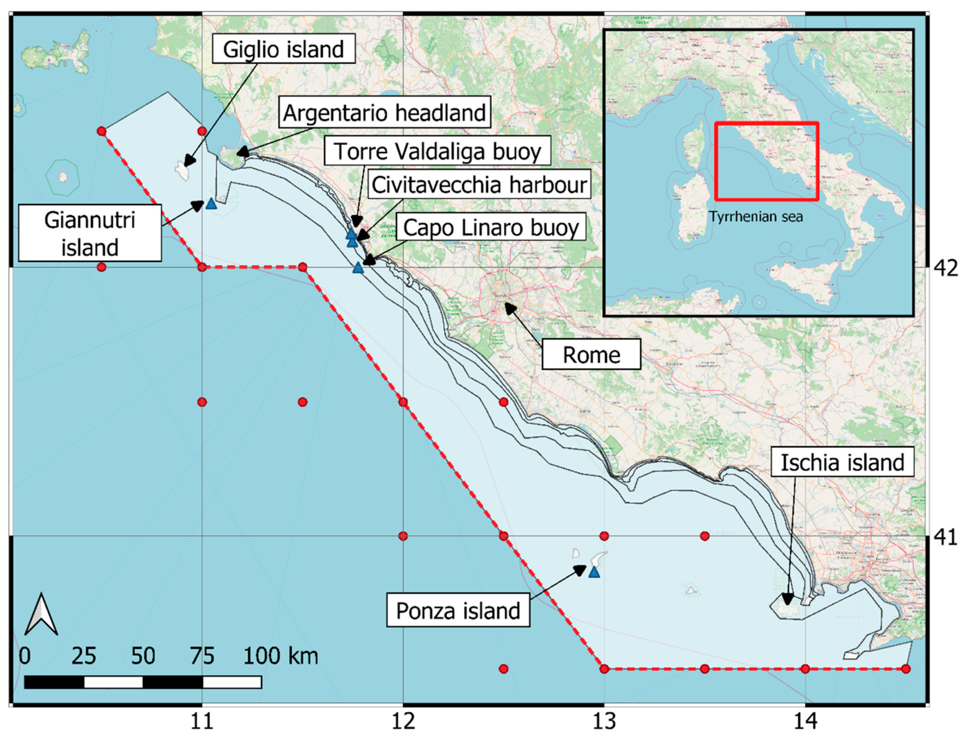
The geographical area of interest is the north-central Tyrrhenian Sea, particularly along the nearly 350 km coasts of the Lazio Region (on the basin eastern side), as can be seen in Figure 1. The semi-enclosed Tyrrhenian Sea exhibits an irregular shape, with the variable shelter of the large island of Sicily from the southerly storms and Sardinia and Corsica from the prevailing westerly storms.
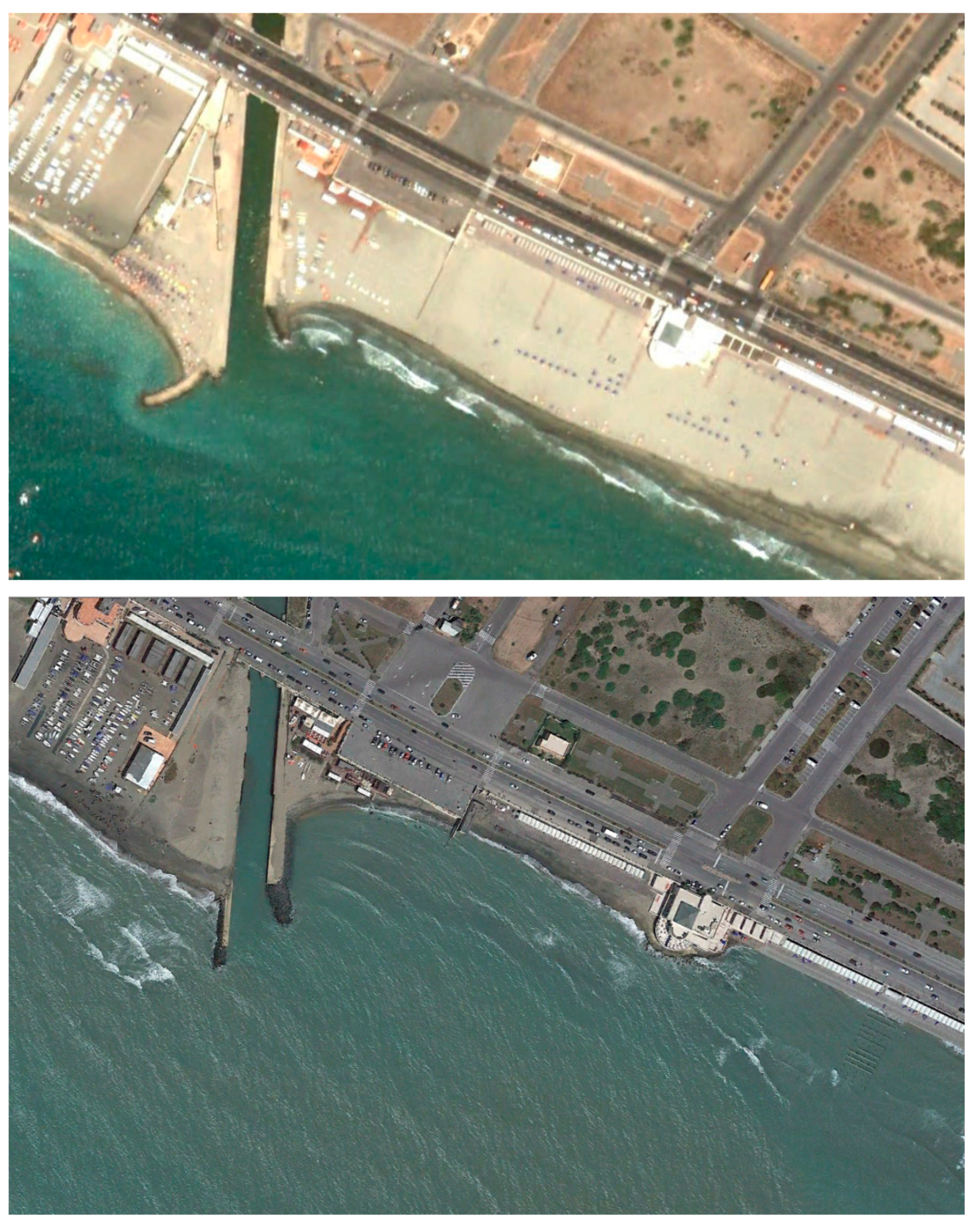
The coastal area is rather variable and complex, due the presence of several small islands at the north and south boundaries, which are included in the model shelter effects. The continental shelf along this coast is quite narrow (around 30 km on average), and the coast shows an alternation of sandy beaches (especially in the central area with the Tiber delta) and rocky coasts and capes (especially near Civitavecchia). Many beaches, particularly at Ostia, very close to Rome, are suffering from severe erosion and are partially protected (see Figure 2 from Google Earth images).
The coastal area is quite close to the large city of Rome, and is rather important, both in terms of economic activities (especially beach tourism and marinas, as well as the large commercial port of Civitavecchia) and in terms of environmental and archaeological values. Nearly 5 million people live in the coastal municipalities facing this area.
2.2. Available Data for Model Validation and Calibration
In the central Tyrrhenian Sea, many direct instrumental wave measurements have been carried out in the past, due to the strategic importance of the corresponding coastal area. Some local measurements by ground-based radar and by satellite altimeters are also available, but have not been considered in this research. All the recording stations are listed in Table 1. It is shown that the buoy records were managed by different authorities at different water depths in different and limited time periods, even with variable sampling intervals. Therefore, they can hardly be used for a consistent characterization of the wave climate at a regional scale. However, all of them have been collected and validated, and then the most reliable and representative ones have been properly used for model validation and calibration.
2.3. Implementation of SWAN Model for Downscaling
SWAN (simulating waves in the nearshore) was selected to model the wave propagation from offshore to inshore. It is open-source, developed by Delft Technical University, and widely used for coastal engineering applications. It is a phase-averaged spectral model that can reproduce most of the phenomena of importance in the nearshore areas, such as wave generation from winds, nonlinear effects in both deep and shallow waters, wave shoaling and refraction, and finally, wave breaking. It can also handle wave diffraction, but since it is based on phase-averaged equations, an approximate model of this phenomenon is adopted.
For the present application, the finite element version of the model is used. This allows us to build a computational domain whose offshore boundary, reproduced as a dashed line in Figure 1, closely follows the position of the offshore points at which the ERA5 wave data are available. It should be noted that in the southern part of the area of interest, the offshore boundary encloses a computational domain larger than what is strictly required by the position of the ERA5 points. This has allowed incorporation of the position of one of the most reliable sources of direct wave measurement in the Mediterranean Sea—the directional wave buoy moored off the Ponza island—thus making possible a very extensive validation of the model results.
The SWAN model is run using a reference frame based on spherical (lat/lon) coordinates. The computational mesh was built using triangular elements, for a total of 8374 points and 15,619 triangles. It had a resolution that increases from offshore toward inshore: the typical size of offshore elements is 10 km, while along the coastline it is 100 m. The wave spectrum at each computational point was discretized using 36 directional and 31 frequency bins (the latter ranging from a minimum of 0.0521 Hz up to a maximum of 1 Hz). The water depth was derived on the basis of the available nautical charts. The effect of the tide, negligible in this microtidal sea, was incorporated, and the computations were carried out with reference to the mean sea level. The time step used for the integration of the equations was 1 h.
Boundary conditions were applied along the offshore boundary on the basis of the ERA5 wave data. For each segment of this boundary, hourly wave data were linearly interpolated using the time series available at each vertex. The ERA5 wave data have been downloaded for the present purposes in terms of some representative sea state parameters, such as the spectral significant wave height, the mean wave period, etc. Then, in order to provide full-frequency direction spectra along the boundary points, a JONSWAP spectra was reconstructed automatically by SWAN, using a peak enhancement factor γ = 3.3.
The wind field of the same ERA5 dataset was used to specify wind velocity and direction over the computational domain, in order to model the local wind wave generation. Note that in the wave model used to produce the ERA5 data, a modified wind field was used in the computations, calculated by applying some minimum values of the wind velocity and further corrections. These data are also made available to Copernicus users at the points of the same grid of the wave model (resolution of 0.5° × 0.5°). In this research, however, in order to use a wind field with better resolution, the wind data of the meteorological parameters of the ERA5 dataset were employed; these were provided on a 0.25° × 0.25° grid.
As far as the modeling of the relevant physical phenomena is concerned, mostly the default values of the SWAN parameters were used. One important exception is the wind wave growth model, for which specific values were adopted. Specifically, a third-generation model was used, in which quadruplet interactions and whitecapping were activated as usual. With reference to Rogers et al., [26], the following set of parameters was employed: a1 = 2.8 × 10⁻⁶, a2 = 3.5 × 10⁻⁵, L = 4.0, and M = 4.0. The standard wind drag formula reported in the cited research is used. For the “windscaling” parameter, also cited in the SWAN manual, the large value of 50.0 was selected. It is in fact well-known that in general, hindcasted wave datasets tend to underestimate the wave energy in the Mediterranean Sea [11]. Therefore, some tentative computations were carried out with some values of this parameter and comparing model results with available buoy measurements. The statistical indexes used for the comparison are described in the next section, but it is anticipated here that the selected value of the “windscaling” parameter is the one that makes the slope index (Equation (3)) more similar to 1 for most of the wave buoys’ locations. Finally, the approximate wave diffraction model was not activated: a reduced ability of the model to carefully reproduce the wave propagation in coastal areas sheltered by small scale obstacles was therefore expected.
The model was run for the whole 42 years period of availability of the ERA5 dataset (1979–2020). From a computational point of view, each year was run independently from the others by using 10 initial days of warm up, as well as by running the last days of the preceding year starting from calm conditions. This allows a perfect parallelization of the model run for each year, taking advantage of distributed memory computational resources, and eventually, networks of independent computers. The computational time for each year, on a standard personal computer (PC) equipped with an Intel Core i7-8700 CPU (3.20 GHz) is of the order of three hours, when dedicating two cores to the process.
The selection of the results to be saved is very important, as the process of writing data to the hard disk can deeply affect the global computational times and complete results for the whole computational grid over the 42 years, and requires a huge amount of disk space. Model outputs are therefore saved in terms of synthetic wave parameters for selected points, where wave measurements are available, and for about 400 points of nearshore locations of interest. Time series are produced with reference to strategic positions of the coastal area, such as in front of the main harbors at different water depths and along the −10 m bottom contour line in front of sandy beaches at a relative distance of the order of 100–1000 m from each other.
3. Results and Model Validation
3.1. Methodology
The model results were validated against selected measurements available at locations inside the numerical domain, using both synchronous and asynchronous comparison methods. The first one was based on the comparison of the predicted wave parameters against the available measured ones at the same time level. The second was based on the comparison, over a time window, of some statistical parameters as, for example, wave frequency tables, wave roses, extreme wave heights of corresponding storms, and maximum annual wave data.
The synchronous comparison of the significant wave height, the mean wave direction, and the mean wave period was carried out between the data predicted by the numerical model and those measured by wave buoys at Ponza, Capo Linaro, Civitavecchia, Giannutri, and Torre Valdaliga. The following statistical parameters have been calculated to evaluate the quality of the comparison, where P refers to predicted wave properties (e.g., significant wave height, mean wave direction, wave period) and O to observations:
In these equations, stands for the standard deviation, and the overstanding bar indicates that the average value is considered; ρ is the Pearson’s correlation coefficient that, if equal to one, measures a positive linear correlation between the two variables considered; NRMSE is the root mean square error normalized by the root mean square of the observed data (smaller values indicate smaller error); and slope is the coefficient indicating the cotangent of the angle between the horizontal and the lines, with zero intercepts, that best fits the data (black solid line in Figure 3). The closer the slope is to one, the better is the comparison. NBIAS is the normalized mean bias factor that represents the mean error divided by the mean value of the observed data. SI is the scatter index that, together with the NRMSE, combines information on both the average and the scatter errors between two datasets. HH is the index proposed by [27].
3.2. Results
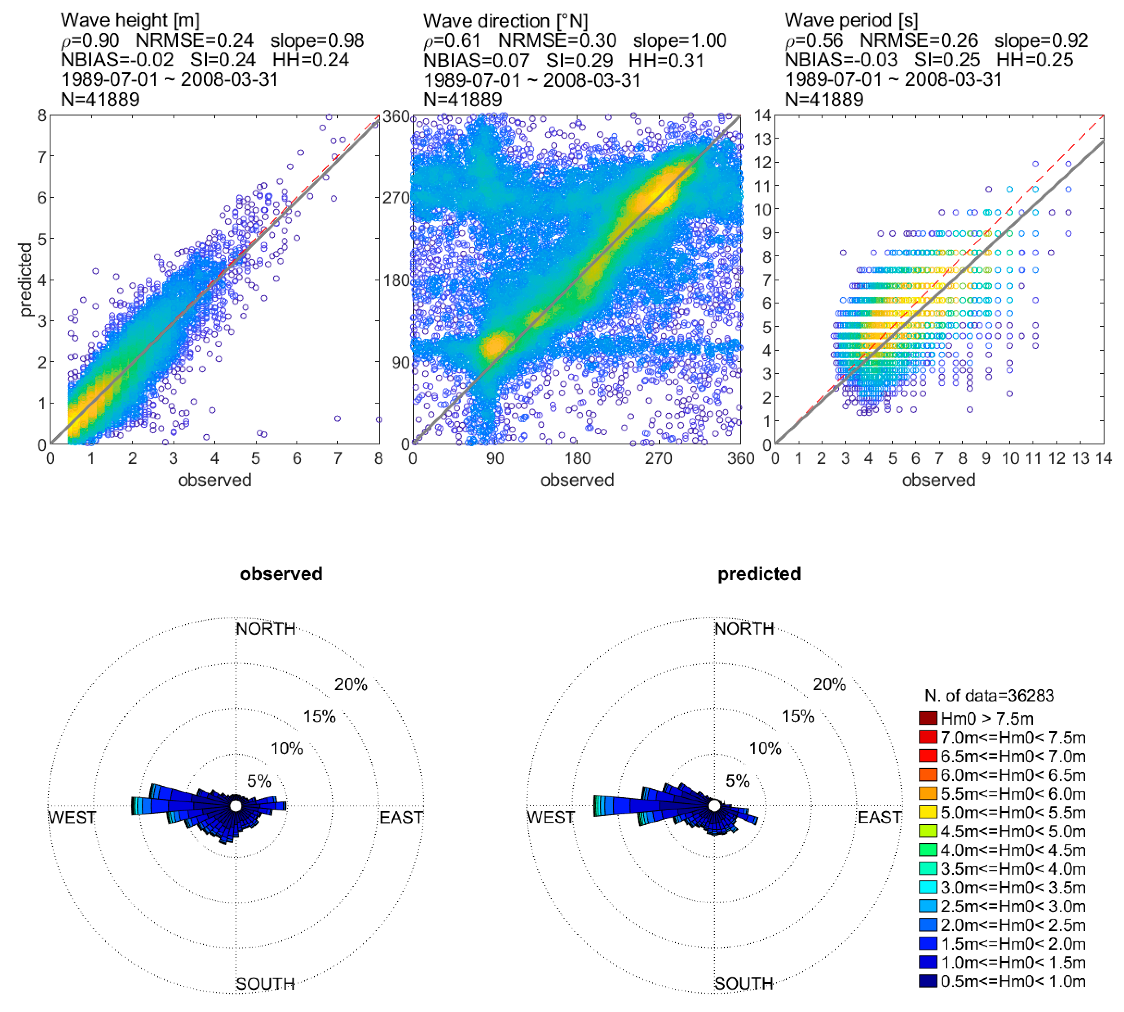
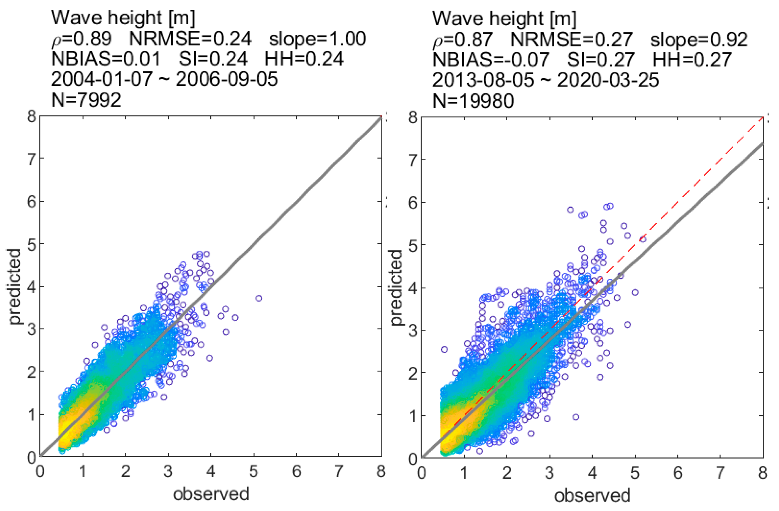
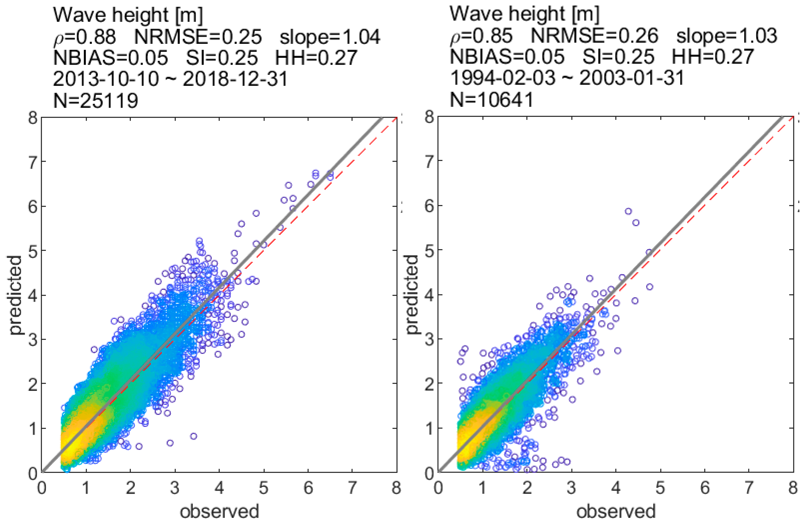
Detailed analysis is shown in Figure 3 for the wave data at the Ponza location, for the Civitavecchia area in Figure 4 and for Giannutri and Torre Valdaliga buoys in Figure 5. A scatter plot is used, where each circle marker represents a sea state as measured by the instrument (x-axis) and as predicted by the model (y-axis). The comparison is optimal for the markers that lay on the bisector (red dashed line). The statistical parameters introduced above are reported for each comparison as the plot title. For the Ponza buoy, the wave climate is also compared by means of the predicted and observed wave rose, while for the sake of brevity, it is not reported for the other buoys.
In general, a very good agreement was found between model predictions and measurements, especially if the significant wave height is considered. For this parameter, the slope of the best fit line (Equation (3)) is very close to 1, with minimum value of 0.92 for the Civitavecchia buoy and maximum of 1.04 for the Giannutri buoy. The scatter index SI (Equation (5)) was between the minimum value of 0.24 for Ponza and Capo Linaro, and the maximum of 0.27 for Civitavecchia. Similar accuracy was found for the other wave parameters. Comparison of the wave roses confirms the ability of the numerical model, coupled to the ERA5 data, of predicting the average wave climate, including the wave direction.
As far as the extreme storms are concerned, a dedicated analysis has been carried out and is briefly described in the following. The idea was to compare the available recorded significant wave height peaks of independent events against those predicted by the numerical model for the same storms, but not necessarily occurring exactly at the same time (asynchronous correlation). For the comparison, the area of Civitavecchia harbour has been selected, where many different wave record measurement sources are available, as introduced before. All the measurements have been converted in the equivalent values at a point offshore Civitavecchia, at a “deep” water depth of −115 m. The conversion has been carried out by evaluating wave shoaling and refraction, as well as on the basis of the correlations that can be worked out using the SWAN model results. Specifically, by applying simple correction coefficients to the measurements of the buoys operating at different water depths, one single equivalent time series offshore Civitavecchia harbour has been derived.
A further correction has been applied to account for the different time resolution of some measurements, by reducing the peak values to those that would have been expected into an hourly wave time series. Specific analysis of the buoy records at the locations of Civitavecchia and Giannutri, where half-hourly data are available, has revealed that the storms peaks (extreme values) of the significant wave heights, in half-hourly time series records, are on average 2.5% higher than those recorded by the hourly time series, and 7.0% higher than from the three-hourly time series. The three-hourly time series (Torre Valdaliga, Montalto di Castro, and part of that at Giannutri) was therefore corrected by multiplying for a further coefficient of 1.05, to account for the higher probability of measuring larger peaks in an hourly time series.
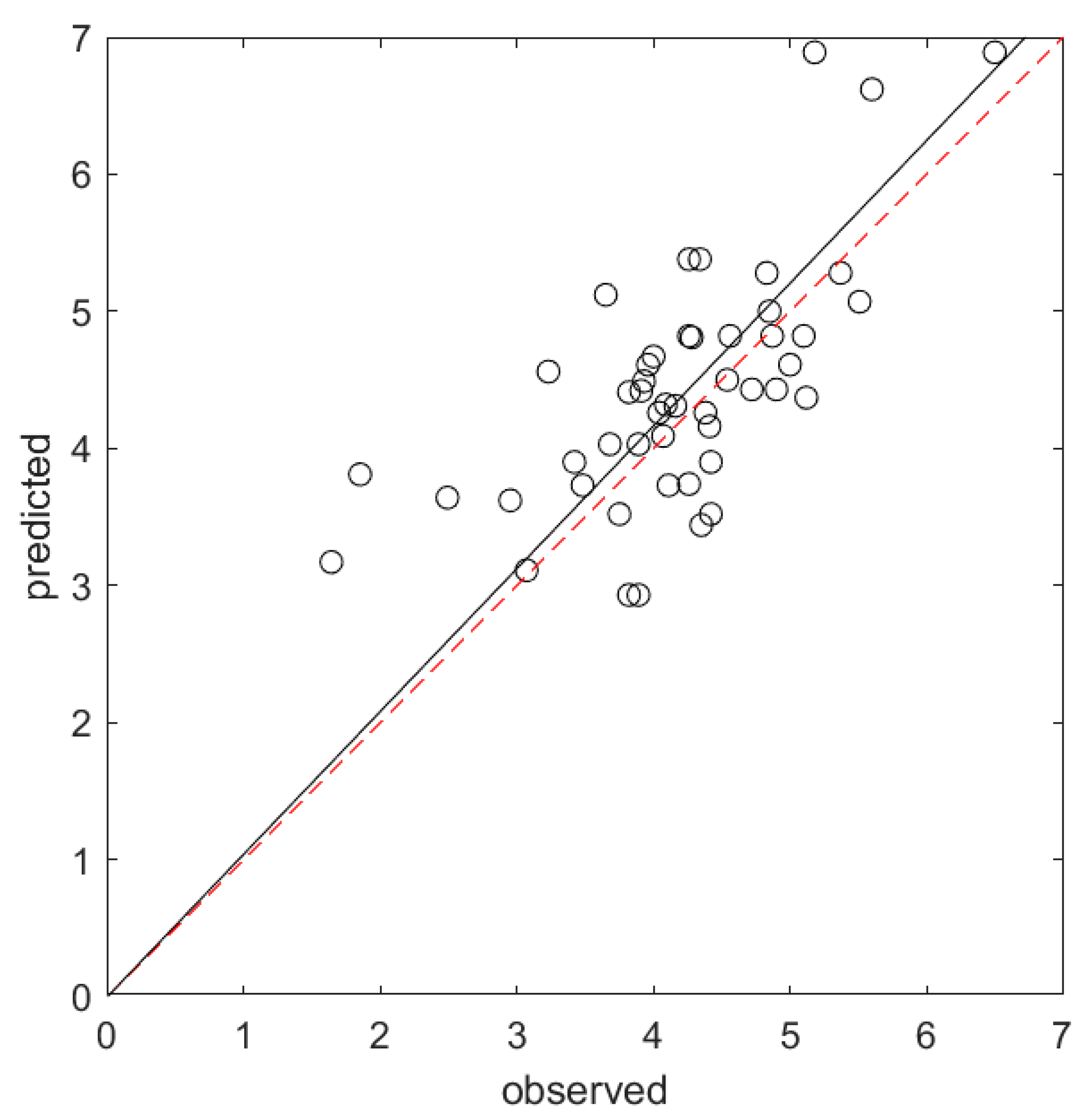
A total of 38 storms has been selected in the time series of the numerical results at the points considered, by using the peaks over threshold (POT) method [28], with a lower limit of Hs = 2.9 m. Each storm was extracted from the available wave measurement records, and the corresponding peak values were collected. For the earlier 22 storms, only one measurement was available; specifically, 11 storms (1980–1994) were extracted from the Montalto di Castro time series, 6 storms (1995–2003) from Torre Valdaliga, and 5 storms (2004–2010) from Capo Linaro. Then, since 2013–2014, the buoys managed by the Port Authority of Civitavecchia and that of Giannutri became simultaneously available. With reference to this period, 16 independent storms were selected. By considering all the available measured peak storms, a total of 49 comparisons can be carried out, some of which, especially after 2014, refer to the same storm as measured by different buoys. The comparison is reported in Figure 6, from which it can be concluded that a very reasonable estimate of the extreme values of the significant wave height is provided by the model. The best fit line of the sample is of 1.0409, indicating a model overestimate of the order of 4%.
By analyzing both the synchronous and asynchronous comparisons, it can be concluded that a SWAN model based on ERA5 boundary conditions and wind fields provides a quite accurate wave hindcast dataset, at least with reference to the coastal area here considered and to the set of model parameters employed. The dataset appears adequate to provide information about wave conditions along the coasts of the central Tyrrhenian Sea at a fine spatial resolution, in terms of both average (climate) conditions and extreme values.
4. Example Application: Evaluation of Potential Coastal Sediment Transport
Wave data are now available with reference to a long time span and with a fine spatial resolution. Several physical input data for coastal engineering and management activities can then be evaluated on this basis. For example, inshore extreme wave properties can be calculated to design coastal structures; inshore wave climate can be used to give detailed interpretation of short- and long-term coastal morphodynamics, and to propose countermeasures against coastal erosion. Further modeling can also be carried out using the inshore wave conditions as a boundary/input parameter, i.e., small-scale hydro/morpho-dynamic models can be applied, as well as short and long-term shoreline evolution models.
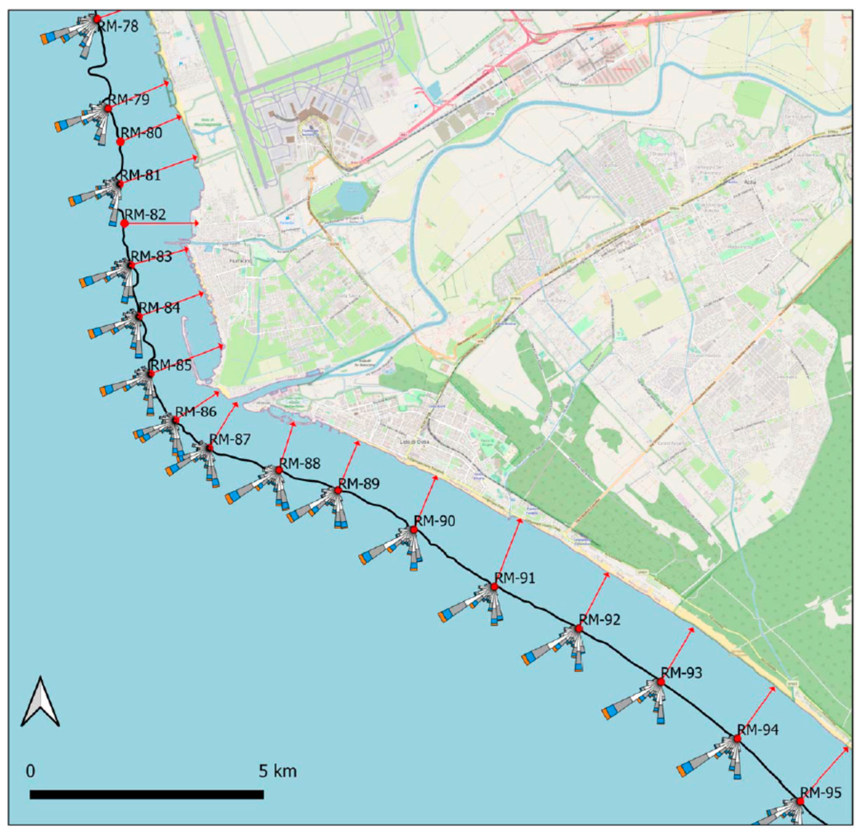
As an example, in this section we show how some parameters and statistics for the support of engineering activities aimed at the mitigation of coastal erosion in the Lazio Region can be evaluated using the present dataset. Fundamental information on the wave height and direction was first derived for each inshore point by constructing and representing the wave roses on a small-scale map (Figure 7). As an example, a portion of the coastal area immediately south of Rome city was considered. As expected, the wave climate in the area was dominated by the waves from the western sector (typically W, SW) and by less intense storms from south (typical incoming offshore direction is S–SE). Due to refraction, accurately taken into account by SWAN model, the inshore wave direction tends to become orthogonal to the coast, especially for the western waves.
Then, the following parameters were evaluated for all the inshore locations:
- (m): significant wave height exceeded 12 h per year;
- (s): significant wave period related to ;
- (m): closure depth;
- (°N): orthogonal to the coastal line;
- (W/m): net longshore energy flux.
The significant wave height exceeded 12 h per year at the inshore locations is calculated from a duration curve, obtained by considering all the Hm0 of the time series. The associated wave period was obtained by considering all the wave conditions for which Hm0 Hm0,12. and fitting an interpolation function on the resulting dataset. The closure depth is calculated using the formula [29]
The longshore energy flux has been calculated for each sea state, considering the angle between each sea state average wave direction, and . The angle is considered clockwise with reference to the north, and is obtained by manually tracking the orthogonal line from each point to the coast (red arrows in the Figure 7). The following formula is used to calculate the wave longshore energy flux for each sea state:
where is the water density (1030 kg/m3), is the gravity acceleration (9.81 m/s2), and 0.6 is the breaking index. The mean energy flux for all the sea states where is named the left longshore energy flux, is positive, and occurs when waves generate a sediment transport toward the left when one is looking at the sea from the coast; the mean flux for is named the right longshore energy flux, and has a negative value. The net energy flux is calculated as the average over the whole time series.
Table 2 reports the values of the synthetic parameters for some representative points shown in Figure 7. While some of them (Hm0,12, Tm0,12, and dclosure) are similar in the considered area, the net longshore energy flux has higher variations, due to the rapidly changing orientation of the shoreline due to the river mouth. Specifically, it is negative in the area north of the river mouth, indicating an energy flux directed toward north. This is expected, as the storms from the west are in this specific area are mostly orthogonal to the coast, while those from south attack the beach at a large angle, generating a relevant energy flux toward the north. In the area south of the river mouth, the net flux is positive, indicating a net energy flux toward the southeast. Here, the storms from the two main sectors have a counteracting effect on the net energy flux, but the western ones appear to dominate. This is coherent with the tendency of the long-term shoreline evolution in the area (see Figure 2).
The energy flux is based on wave data at −10 m, and therefore carefully take into account refraction and shoaling effects. It can also be used to evaluate the potential sediment transport flux, by specifying sediment properties and by applying one of the available formulae, as for example the one that was developed at CERC [30].
5. Limitations of the Procedure and Discussion
The downscaling procedure appears to provide a very reliable dataset for nearshore applications. However, in order to also provide warning and guidance for its application in different areas, a couple of points are discussed in this section: (i) how boundary conditions are specified, starting from bulk wave parameters, and (ii) how calibration is carried out.
Statistical (bulk) parameters describing each sea state (i.e., significant wave height and period, mean wave direction, spectral peak width) available from the ERA5 dataset at the vertexes of the offshore limit of the domain are used to build a synthetic JONSWAP spectrum at each boundary computational point. This procedure does not take therefore into account the specific spectral shape reconstructed by the wave model used to build the ERA5 results. It is clear that if the wave spectrum differs too much from a standard JONSWAP one, the accuracy of the results can be negatively affected. This is expected to be of relevance in the case of multimodal seas [31], a condition typically encountered in large ocean basins where locally generated wind waves are superposed to swell. The wave climate in the area of interest is typically unimodal; thus, the use of bulk wave parameters is expected to not affect the results. However, when applying the present procedure to regions where complex (multimodal) spectral shapes are frequent, a careful evaluation of the effects of such a simplification should be carried out. A possible alternative solution could be based on the use of some representative spectrum extracted from the ERA5 database, to be associated to each set of offshore wave parameters, as for example in the hybrid method by Camus et al. [12]. In principle, it is also possible to extract from the ERA5 the spectrum for each point and for each time step, in order to provide the required boundary conditions. However, in the authors’ opinion, this is not practical, as the required computational resources would grow indefinitely.
The second point of discussion concerns the calibration procedure. It is well-known that global models tend to underestimate the intensity of wind fields, and therefore the wave energy [11]. Before use of these data, and before applying any downscaling procedure, a calibration is therefore always recommended. This is carried out by comparing the model results with measurements (in situ or remote; for example, in [12,32]) and by accordingly correcting the global model results. In the present research, a different approach has been tested, due to the fact that most of the direct wave measurements used are available at locations very close to the coast, i.e., far from the ERA5 data points. The ERA5 data have been used as boundary conditions without applying a correction factor; calibration has been carried out by varying the parameters of the wind wave generation model incorporated in SWAN, as detailed in Section 2.3. This procedure has the effect that the model that accounts for the transfer of energy from wind to waves is boosted to compensate for the deficit of wave energy at the boundaries of the computational domain, and of the wind speed that forces the local wave generation. This could lead to spectral shapes with enhanced high-frequency tails with respect to the actual ones, in view of the augmented local sea. However, comparison with nearshore buoy data has shown very satisfactory results in terms of bulk wave parameters, as shown in Section 3.
6. Conclusions
In this paper, an example application of coastal regional downscaling of the Copernicus ERA5 wave dataset has been described. The data have been used as input for the SWAN wave model, able to model the wave generation and propagation in coastal areas. On the basis of the computations, a further dataset, containing wave time series at the inshore computational points, has been produced. It has been validated against available wave measurements, and it appears that, after a preliminary calibration of the wave generation module of SWAN, a very reasonable agreement can be obtained between measurements and dataset. The data, covering some 42 years, can be expanded by updating the dataset on a regular basis, as the ERA5 become available. This is done by the ECMWF every few days, typically once per week. Furthermore, a preliminary version of the data has just been released, back to the fifties.
The inshore wave time series are then available for typical engineering and management activities. Among the possible uses, it is foreseen that a time series of potential solid transport can be built, also following some of the ideas reported in the Section 4, where calculation of longshore wave energy flux has been presented for a sample area. However, the main goal of this research is to present a modeling chain that allows us to deal with engineering and management coastal activities, starting from a well-validated, meteoceanographic dataset. Further models can also be run using the inshore wave time series. For example, simplified shoreline evolution models might be run with reference to the 42 years, producing a hindcasted shoreline position time series with high spatial resolution. These might be very useful for coastal engineering design projects, both to evaluate past trends and to model the effect of design solutions for the mitigation of the coastal erosion.
It is finally noted that meteoceanographic parameters, such those considered here, with high spatial and temporal resolution, appear to be (see [1]) some of the fundamental inputs for operational coastal services, to be shortly developed at the Italian national level as downstream products of Copernicus Core Services.
Author Contributions
Conceptualization, G.B. and L.F.; methodology, G.B. and C.C.; software, G.B. and C.C.; validation, G.B., L.F. and C.C.; formal analysis, G.B. and L.F.; writing—original draft preparation, G.B., L.F. and C.C.; writing—review and editing, G.B., L.F. and C.C.; visualization, C.C.; supervision, G.B. and L.F. All authors have read and agreed to the published version of the manuscript.
Funding
This research has not received specific external funding, but has been developed to achieve common scientific objectives in a joint research with the Italian regional authority Regione Lazio.
Institutional Review Board Statement
Not applicable.
Informed Consent Statement
Not applicable.
Data Availability Statement
The data presented in this study are available on request from the corresponding author.
Acknowledgments
Fruitful exchanges of ideas with G. Besio on wave hindcasting in the Mediterranean Sea are gratefully acknowledged. The ERA5 has been generated under the Copernicus Climate Change Service of the Copernicus Programme. The dataset “ERA5 hourly data on single levels from 1979 to present” has been downloaded from the Climate Data Store.
Conflicts of Interest
The authors declare no conflict of interest.
References
- Geraldini, S.; Bruschi, A.; Bellotti, G.; Taramelli, A. User needs analysis for the definition of Operational Coastal services. Water 2021, 13, 92. [Google Scholar] [CrossRef]
- The WAMDI Group. The WAM Model—A Third Generation Ocean Wave Prediction Model. J. Phys. Oceanogr. 1988, 18, 1775–1810. [Google Scholar] [CrossRef] [Green Version]
- Komen, G.J.; Cavaleri, L.; Donelan, M.; Hasselmann, K.; Hasselmann, S.; Janssen, P.A.E.M. Dynamics and Modelling of Ocean Waves; Cambridge Univ. Press: Cambridge, UK, 1994. [Google Scholar]
- Gunther, H.; Hasselmann, S.; Janssen, P.A.E. The WAM model Cycle 4; Report No. 4; DKRZ: Hamburg, Germany, 1992. [Google Scholar]
- Tolman, H.L. User Manual and System Documentation of WAVEWATCH-III Version 1.15; NOAA/NWS/NCEP/OMB Technical Note; National Oceanic and Atmospheric Administration: Washington, DC, USA, 1997; Volumes 97, 151.
- Tolman, H.L. User Manual and System Documentation of WAVEWATCH III Version 4.18; NOAA/NWS/NCEP/MMAB Technical Note; National Oceanic and Atmospheric Administration: Washington, DC, USA, 2014; p. 316.
- The WAVEWATCH III Development Group. User Manual and System Documentation of WAVEWATCH III Version 5.16; NOAA/NWS/NCEP/MMAB Technical Note; National Oceanic and Atmospheric Administration: Washington, DC, USA, 2016; Volume 329, 326p.
- Booij, N.; Ris, R.C.; Holthuijsen, L.H. A third generation wave model for coastal regions: 1. Model description and validation. J. Geophys. Res. Ocean 1999, 104, 7649–7666. [Google Scholar] [CrossRef] [Green Version]
- Ris, R.C.; Holthuijsen, L.H.; Booij, N. A third generation wave model for coastal regions: 2. Verification. J. Geophys. Res. Ocean 1999, 104, 7667–7681. [Google Scholar] [CrossRef]
- Reguero, B.G.; Menéndez, M.; Méndez, F.J.; Mínguez, R.; Losada, I.J. A Global Ocean Wave (GOW) calibrated reanalysis from 1948 onwards. Coast. Eng. 2012, 65, 38–55. [Google Scholar] [CrossRef]
- Cavaleri, L.; Sclavo, M. The calibration of wind and wave model data in the Mediterranean Sea. Coast. Eng. 2006, 53, 613–627. [Google Scholar] [CrossRef]
- Camus, P.; Mendez, F.J.; Medina, R.; Tomas, A.; Izaguirre, C. High resolution downscaled ocean waves (DOW) reanalysis in coastal areas. Coast. Eng. 2013, 72, 56–68. [Google Scholar] [CrossRef]
- Breivik, O.; Gusdal, Y.; Furevik, B.R.; Johan Aarnes, O.; Reistad, M. Nearshorewave forecasting and hindcasting by dynamical and statistical downscaling. J. Mar. Syst. 2009, 78 (Suppl. S1), S235–S243. [Google Scholar] [CrossRef] [Green Version]
- Gaslikova, L.; Weisse, R. Estimating near-shore wave statistics from regional hindcasts using downscaling techniques. Ocean Dyn. 2006, 56, 26–35. [Google Scholar] [CrossRef]
- Saviano, S.; De Leo, F.; Besio, G.; Zambianchi, E.; Uttieri, M. HF Radar Measurements of Surface Waves in the Gulf of Naples (Southeastern Tyrrhenian Sea): Comparison with Hindcast Results at Different Scales. Front. Mar. Sci. 2020, 7. [Google Scholar] [CrossRef]
- Camus, P.; Mendez, F.J.; Medina, R. A hybrid efficient method to downscale wave climate to coastal areas. Coast. Eng. 2011, 58, 851–862. [Google Scholar] [CrossRef]
- Browne, M.; Castelle, B.; Strauss, D.; Tomlinson, R.; Blumenstein, M.; Lane, C. Near-shore swell estimation from a global wind-wave model: Spectral process, linear, and artificial neural network models. Coast. Eng. 2007, 54, 445–460. [Google Scholar] [CrossRef] [Green Version]
- Kalra, R.; Deo, M.C.; Kumar, R.; Agarwal, V.K. Artificial neural network to translate offshore satellite wave data to coastal locations. Ocean Eng. 2005, 32, 1917–1932. [Google Scholar] [CrossRef]
- Menendez, M.; García-Díez, M.; Fita, L.; Fernández, J.; Méndez, F.J.; Gutiérrez, J.M. High-resolution sea wind hindcasts over the Mediterranean area. Clim. Dyn. 2014, 42, 1857–1872. [Google Scholar] [CrossRef]
- Mentaschi, L.; Besio, G.; Cassola, F.; Mazzino, A. Developing and validating a forecast/hindcast system for the Mediterranean Sea. J. Coast. Res. 2013, 65, 1551–1556. [Google Scholar] [CrossRef]
- Hersbach, H.; Bell, B.; Berrisford, P.; Hirahara, S.; Horányi, A.; Muñoz-Sabater, J.; Nicolas, J.; Peubey, C.; Radu, R.; Schepers, D.; et al. The ERA5 global reanalysis. Q. J. R. Meteorol. Soc. 2020, 146, 1999–2049. [Google Scholar] [CrossRef]
- Cappucci, S.; Scarcella, D.; Rossi, L.; Taramelli, A. Integrated coastal zone management at Marina di Carrara Harbor: Sediment management and policy making. J. Ocean Coast. Manag. 2011, 54, 277–289. [Google Scholar] [CrossRef]
- Cappucci, S.; Bertoni, D.; Cipriani, L.E.; Boninsegni, G.; Sarti, G. Assessment of the Anthropogenic sediment budget of a littoral cell system (Northern Tuscany, Italy). Water 2020, 12, 3240. [Google Scholar] [CrossRef]
- Taramelli, A.; Cappucci, S.; Valentini, E.; Rossi, L.; Lisi, I. Nearshore Sandbar Classification of Sabaudia (Italy) with LiDAR Data: The FHyL Approach. Remote Sens. 2020, 12, 1053. [Google Scholar] [CrossRef] [Green Version]
- Cappucci, S.; Vaccari, M.; Falconi, M.; Tudor, T. The sustainable management of sedimentary resources. “The case study of Egadi Project”. Environ. Eng. Manag. J. 2019, 18, 317–328. [Google Scholar]
- Rogers, W.E.; Babanin, A.V.; Wang, D.W. Observation-consistent input and whitecapping dissipation in a model for wind-generated surface waves: Description and simple calculations. J. Atmos. Ocean. Technol. 2012, 29, 1329–1346. [Google Scholar] [CrossRef]
- Hanna, S.R.; Heinold, D.W. Development and Application of a Simple Method for Evaluating Air Quality; Tech. Rep.; American Petroleum Institute, Health and Environmental Affairs Department: Washington, DC, USA, 1985. [Google Scholar]
- Goda, Y. On the methodology of selecting design wave height. Coast. Eng. 1988, 899–913. [Google Scholar] [CrossRef] [Green Version]
- Hallermeier, R.J. A profile zonation for seasonal sand beaches from wave climate. Coast. Eng. 1981, 4, 253–277. [Google Scholar] [CrossRef]
- Shore Protection Manual (SPM), 4th ed.; Vicksburg, Mississippi Military Department of the Army, Waterways Experiment Station, Corps of Engineers, Coastal Engineering Research Center: Washington, DC, USA, 1984; Volume 2.s.
- Hegermiller, C.A.; Antolinez, J.A.A.; Rueda, A.; Camus, P.; Perez, J.; Erikson, L.H.; Barnard, P.L.; Mendez, F.J. A multimodal wave spectrum-based approach for statistical downscaling of local wave climate. J. Phys. Oceanogr. 2017, 47, 375–386. [Google Scholar] [CrossRef]
- Mínguez, R.; Espejo, A.; Tomás, A.; Méndez, F.J.; Losada, I.J. Directional calibration of wave reanalysis databases using instrumental data. J. Atmos. Ocean Technol. 2011, 28, 1466–1485. [Google Scholar] [CrossRef]
Figure 1.
Geographical area of interest. The white area represents the computational domain of the SWAN (simulating waves in the nearshore) model, red dots the nodes where the ERA5 data are available, blue triangles the location of the wave buoys used. Simplified bottom contour lines for water depths of −10, −20, −50, −100 m are also shown.

Figure 2.
Beach erosion at the Canale dei Pescatori inlet at Ostia (Rome). Upper figure: July 2003, after a large, unprotected sand nourishment. Lower figure: April 2017. Approximate size of the framed area: 500 × 320 m. North is aligned with upwards direction of the figure. Both figures are taken from the Google Earth web site

Figure 3.
Wave data at the Ponza buoy. On the top is a comparison between observed and predicted significant wave height, mean wave direction, and mean wave period. At the bottom are observed (left) and predicted (right) wave climate in terms of wave roses.
Figure 3.
Wave data at the Ponza buoy. On the top is a comparison between observed and predicted significant wave height, mean wave direction, and mean wave period. At the bottom are observed (left) and predicted (right) wave climate in terms of wave roses.

Figure 4.
Comparison of significant wave height predicted and measured at Capo Linaro (left) and Civitavecchia CVT1 (right).
Figure 4.
Comparison of significant wave height predicted and measured at Capo Linaro (left) and Civitavecchia CVT1 (right).

Figure 5.
Comparison of significant wave height predicted and measured at Giannutri (left) and Torre Valdaliga (right) buoys.
Figure 5.
Comparison of significant wave height predicted and measured at Giannutri (left) and Torre Valdaliga (right) buoys.

Figure 6.
Peak significant wave height for independent storms, as recorded by six wave buoys (observed) and predicted by the numerical model. Red dashed line represents ideal agreement between the two data sets. Black line is the best fit with slope of 1.0409.
Figure 6.
Peak significant wave height for independent storms, as recorded by six wave buoys (observed) and predicted by the numerical model. Red dashed line represents ideal agreement between the two data sets. Black line is the best fit with slope of 1.0409.

Figure 7.
Nearshore wave roses along the Rome–Ostia coastal area—an example application to a portion of the model domain. Red arrows represent the local orthogonal to the coast.
Figure 7.
Nearshore wave roses along the Rome–Ostia coastal area—an example application to a portion of the model domain. Red arrows represent the local orthogonal to the coast.


Table 1.
Existing wave buoy measurements in the area (see map in Figure 1). Wave data in italics was not used in this study.
Table 1.
Existing wave buoy measurements in the area (see map in Figure 1). Wave data in italics was not used in this study.
| Station Location | Owner/Manager | Depth. (m) | Information | Time Coverage |
|---|---|---|---|---|
| Ponza | APAT—RON | 100 | Directional; 3-hourly up to 2002, then ½-hourly | July 1989–March 2008 |
| Torre Valdaliga TV | ENEL—CRIS | −35 | Directional; 3-hourly, 1-hourly for Hs > 2 or 0 m, respectively | February 1994–March 2003 |
| Montalto di Castro | ENEL—CRIS | −50 | Non-directional, 3-hourly | 1976–1994 |
| Capo Linaro | APAT—RON | −100 | Directional, every ½-hourly | February 2004–September 2006 |
| Civitavecchia (nord) TVN | ISPRA—RON | −70 | Directional, ½-hourly | July 2009–September 2014 |
| Civitavecchia CVT1 | Civitavecchia Port Authority | −60 | Directional, ½-hourly | from November 2012 |
| Civitavecchia CVT2 | Civitavecchia Port Authority | −40 | Directional, ½-hourly | November 2012–June 2016 |
| Giannutri | SIRT Tuscany Region | −140 | Directional, ½-hourly | from December 2013 |
| Ostia | Ministry of Infrastructures and Transport of Italy | −12 | Directional, 3-hourly | 1990–1992 |
Table 2.
Wave parameters at significant positions located at −10 m (see Figure 7).
Table 2.
Wave parameters at significant positions located at −10 m (see Figure 7).
| Point | dclosure (m) | Left F (W/m) | Right F (W/m) | Net F (W/m) | |||
|---|---|---|---|---|---|---|---|
| RM-79 | 3.40 | 7.1 | 6.2 | 245 | 964 | −1339 | −375 |
| RM-81 | 3.44 | 7.1 | 6.2 | 248 | 844 | −1487 | −643 |
| RM-83 | 3.47 | 7.1 | 6.3 | 252 | 720 | −1591 | −871 |
| RM-85 | 3.57 | 7.2 | 6.4 | 246 | 843 | −1914 | −1071 |
| RM-87 | 3.63 | 7.3 | 6.5 | 209 | 2310 | −2159 | 151 |
| RM-89 | 3.48 | 7.2 | 6.3 | 200 | 1921 | −1621 | 300 |
| RM-91 | 3.52 | 7.2 | 6.4 | 199 | 1982 | −1408 | 574 |
| RM-93 | 3.39 | 7.1 | 6.1 | 209 | 1598 | −1332 | 266 |
Publisher’s Note: MDPI stays neutral with regard to jurisdictional claims in published maps and institutional affiliations. |
© 2021 by the authors. Licensee MDPI, Basel, Switzerland. This article is an open access article distributed under the terms and conditions of the Creative Commons Attribution (CC BY) license (http://creativecommons.org/licenses/by/4.0/).
Share and Cite
MDPI and ACS Style
Bellotti, G.; Franco, L.; Cecioni, C. Regional Downscaling of Copernicus ERA5 Wave Data for Coastal Engineering Activities and Operational Coastal Services. Water 2021, 13, 859. https://doi.org/10.3390/w13060859
AMA Style
Bellotti G, Franco L, Cecioni C. Regional Downscaling of Copernicus ERA5 Wave Data for Coastal Engineering Activities and Operational Coastal Services. Water. 2021; 13(6):859. https://doi.org/10.3390/w13060859
Chicago/Turabian StyleBellotti, Giorgio, Leopoldo Franco, and Claudia Cecioni. 2021. "Regional Downscaling of Copernicus ERA5 Wave Data for Coastal Engineering Activities and Operational Coastal Services" Water 13, no. 6: 859. https://doi.org/10.3390/w13060859
Note that from the first issue of 2016, this journal uses article numbers instead of page numbers. See further details here.