
Computing the Beta Parameter in IDW Interpolation by Using a Genetic Algorithm


1
Department of Civil Engineering, Transilvania University of Brașov, 5 Turnului Street, 900152 Brașov, Romania
2
Department of Mathematics and Computer Science, Ovidius University of Constanta, 124 Mamaia Av., 900527 Constanta, Romania
*
Author to whom correspondence should be addressed.
Water 2021, 13(6), 863; https://doi.org/10.3390/w13060863
Submission received: 14 January 2021
/
Revised: 22 February 2021
/
Accepted: 20 March 2021
/
Published: 22 March 2021
(This article belongs to the Special Issue Assessing Water Quality by Statistical Methods)
Abstract
:This article proposes a new approach for determining the optimal parameter (β) in the Inverse Distance Weighted Method (IDW) for spatial interpolation of hydrological data series. This is based on a genetic algorithm (GA) and finds a unique β for the entire study region, while the classical one determines different βs for different interpolated series. The algorithm is proposed in four scenarios crossover/mutation: single-point/uniform, single-point/swap, two-point/uniform, and two-point swap. Its performances are evaluated on data series collected for 41 years at ten observation sites, in terms of mean absolute error (MAE) and mean standard error (MSE). The smallest errors are obtained in the two-point swap scenario. Comparisons of the results with those of the ordinary kriging (KG), classical IDW (with β = 2 and the optimum beta found by our algorithm), and the Optimized IDW with Particle Swarm Optimization (OIDW) for each study data series show that the present approach better performs in 70% (80%) cases.
1. Introduction
Evaluating and predicting the effects of atmospheric factors dynamics, like precipitation and temperature, are of major importance for human activity, especially for zones with arid or rainy climates. Since water scarcity impacts billions of people worldwide, it is important to assess the water resources availability at ungauged locations [1]. Spatial interpolation methods are utilized for estimating the values of environmental variables using data recorded at neighbor locations. The most utilized approaches are classified as deterministic, geostatistical, and combined (or hybrid) [2,3]. The Inverse Distance Weighting (IDW) is a deterministic (mechanical) technique. The attribute values of any pair of points are related to each other, their similarity being inversely proportional to the distance between the two locations [4,5].
Since IDW does not involve advanced computational knowledge, researchers widely utilized it for spatial interpolation problems. Different authors presented comparable IDW performances with other spatial interpolation methods [6,7,8,9,10,11]. In [6,7], it is shown that IDW provided better or comparative results as ordinary kriging (OK) in the spatial interpolation of precipitation in Taiwan and Norfolk Island. Ly et al. [8] reported that OK and IDW provided the smallest root mean squared error in a study concerning the daily rainfall at the catchment scale in Belgium. Dong et al. [9] found that Ordinary CoKriging (OCK) performed better than OK and IDW when interpolating daily rainfall in a river basin from China. IDW, Thiessen Polygons Method (TPM), and kriging have been evaluated against the Most Probable Precipitation Method (MPPM) on annual, monthly, seasonal, and annual monthly maximum precipitation series from ten stations of 41 data [10]. IDW over performed TPM and OK, but underperformed MPPM. Chen et al. [11] proposed an improved regression-based scheme (PCRR) that was superior to IDW and multiple linear regression (MLR) interpolation methods on data from the mesoscale catchment of the Fuhe River.
Even if the classical IDW (with the value of the parameter β = 2) was successfully employed for a long period for spatial interpolation problems, being easy to use, improving its performances was targeted by scientists. For example, Lu and Wong [4] proposed the weights’ modification depending on the neighboring locations’ distribution density around the unsampled place. Golkhatmi et al. [12] introduced altitude as a new variable in the IDW interpolation (keeping β = 2) and reported good results in the case study.
Another direction is finding the best β. This is an optimization problem by itself, targeted by many scientists [13,14,15,16,17,18,19]. For example, Noori et al. [13] employed IDW for estimating the distribution of precipitation in Iran, the value of the parameter (β) being recursively searched in the interval (1, 5], increasing its value each time. However, this grid-search procedure is time-consuming for small step sizes [5]. To avoid this drawback, Mei et al. [14] designed and implementing parallel adaptive inverse distance weighting (AIDW) interpolation algorithms by using the graphics processing unit (GPU) for accelerating the parameter finding. Gholipour et al. [15] propose a hybridization of IDW with a harmony search, which improves the convergence rate and reduces the search time.
In the same idea, hybrid methods have been proposed. Zhang et al. [16] combined Support Vector Machines (SVM) with IDW obtaining the SVM residual IDW, obtaining superior results by comparison to IDW and OK for the spatial interpolation of the multi-year average annual precipitation in the Three Gorges Region basin. Nourani et al. [17] used a two-stage framework for spatial interpolation of precipitation, employing, in the first stage, three artificial intelligence models that generate the input for the second stage, where they utilize IDW for spatial interpolation. Bărbulescu et al. [18] proposed a Particle Swarm Optimization approach (called OIDW) for finding a single β in IDW interpolation of maximum annual precipitation from the Dobrogea region (Romania). Chang et al. [19] applied a genetic algorithm (GA) to find the optimal distances between the gauged stations to minimize the estimation errors in IDW. Still, based on our knowledge, no attempt to optimize the choice of β parameter of IDW using a GA has been made so far.
On the other hand, GAs are widely used for solving real-life problems. For example, Ratnam et al. [20] improved seasonal air temperature forecasts using a genetic algorithm. Nasseri et al. [21] presented an optimized scenario for rainfall forecasting using a genetic algorithm coupled with an artificial neural network using rainfall hyetograph of recording rain gauges in the Upper Parramatta catchment (Sydney, Australia). Using the ability of GAs to search complex decision spaces, Sen and Ôztopal [22] utilized such an algorithm for optimizing the classification of rainy and non-rainy day occurrences using atmospheric data (temperature, humidity, dew point, vertical velocity). Heat conduction and control problems have also been solved by utilizing GAs [23,24].
In this context, this article proposes a new approach that optimizes the finding of the beta parameter of IDW. This is based on a genetic algorithm and finds a unique β for the entire study region, while the classical one determines different βs for different interpolated series. The algorithm is proposed in four scenarios crossover/mutation: single-point/uniform, single-point/swap, two-point/uniform, and two-point swap. Comparisons of its performances with those of the classical IDW (with β = 2 and the optimal beta found in our algorithm), ordinary kriging, and two versions of the optimized IDW by using Particle Swarm Optimization (OIDW) are also provided.
2. Methodology and Data Series
2.1. IDW Interpolation
The study problem is estimating a variable’s values at ungagged locations employing the same variable’s known values, registered at the neighboring observation sites [18]. In terms of mathematics, one can formulate the problem as follows. Given a set of spatial data of a variable z at n observation sites, determine the same variable’s values at the study site,
The IDW interpolation formula is:
where is the value computed for the site , is the value recorded at the site , is the distance between and, and β is a parameter whose value is either given or determined by different optimization methods. In the original algorithm, β = 2 [25,26].
The interpolation quality depends on which is generally determined after running a grid search. The time spent for finding the parameters is inverse proportional with the step of the grid.
2.2. Genetic Algorithms
A genetic algorithm (GA) is a metaheuristic method inspired by natural selection laws that try to find optimal solutions to complex problems to which deterministic approaches usually cannot find a good result. The genetic operators, selection, crossover, and mutation establish a balance between the exploration and exploitation of the search space [27,28]. Exploration means that the algorithm searches for new solutions in new regions, while exploitation refers to making refinement to existing solutions to improve their quality. A function called fitness measures the quality of the solutions, which are represented by chromosomes.
A GA starts with a population of some random chromosomes and (by applying the principle of ’survival of the fittest’) produces multiple generations by selecting in each one the fittest individuals for breeding. The mutation is then applied to increase the population diversity. Along with the generations, better individuals, i.e., better approximations to the solution, are obtained. The process continues until the fittest individual (the optimal solution) is found or the maximum number of generations is reached.
Using a genetic algorithm to solve a problem means finding the representation of the problem’s solutions (encoding of the chromosomes), the fitness function, and the genetic operators. A chromosome is a feasible solution to the problem. In our case, a chromosome represents a real value of the parameter a ≤ β ≤ b. Thus, we apply a value encoding and get a binary string with the length l, calculated using the following formula (the default encoding of real values to binary strings):
where z represents the given number of β’s decimals. In this study, l = 9 bits.
2l− 1 < (b − a) ∗ 10z < 2l
The decimal value, val, of the binary chromosome representation, is computed by (3). We get the real value of a chromosome (β) by applying (4).
or
val = (β − a) × (2l − 1)/(b − a)
β = a + val × (b − a)/(2l − 1)
The fitness function controls the possibility of individuals’ reproduction. The better chromosome is (i.e., the better fitness is), the more likely it is to be selected for breeding the next generation. Since our goal is to minimize the error between the results obtained by the spatial interpolation and those recorded at the meteorological stations, the fitness function will record the mean standard error (MSE) between the known data and those computed by IDW. A GA performs best when a feasible solution maximizes the fitness function. Hence, we apply one of the most commonly adopted fitness mapping (inversion scaling), which does not alter the minimum location, but converts a minimization problem to an equivalent maximization one.
We use the mean standard error and mean absolute deviation (MAE) to evaluate the GA’s performance. The lowest the MAE or MSE is, the better the algorithm performs.
Genetic operators are used for producing new generations of individuals with more diverse properties. There are three operators, selection, crossover, and mutation, which can set and, most of the time, find a good ratio between exploration and exploitation of the search space.
A selection operator determines the best individuals’ regions that will exchange information to create a new generation. In this paper, the roulette wheel selection method [27] is used.
A crossover operator combines two or more parents to generate one or two offspring. It implements the idea that a swap of information between good individuals will generate an even better one. In this paper, the single-point crossover and the two-point crossover are used to create new offspring [29].
A mutation operator randomly modifies chromosomes with a given probability, pm, called mutation rate, leading to an increased population’s structural diversity. Thus, a mutation operator facilitates the recovery of genetic material lost during the selection step and exploring new solutions. Here we used the uniform mutation [27] (one gene is randomly chosen and its value is modified) and swap mutation [27] (two positions on the chromosome are randomly selected, and their values are interchanged).
One may configure several control parameters in a genetic algorithm to achieve a balance between exploration and exploitation. If the population size is large, the search space is more explored than when the population size is small [28]. However, the runtime of the algorithm would increase. If crossover and mutation rates are high, the search will explore much of the solutions space, but there is a high chance of missing good solutions, the GA acting more like a random search. If crossover and mutation rates are low, the search space remains unexplored, and in this case, the GA resembles the hill-climbing algorithms. Therefore, we investigated the influence of the population size, crossover rate, mutation rate, and stop condition on the GA results. We performed each test ten times and averaged the results to increase their precision (as suggested in the literature). We implemented two crossover operators and two mutation operators to find the ones which are best suited for our problem. We also ran several tests for each pair of operators to see the relationship between the control parameters and the fitness value. Details are presented in the following sections.
2.3. New Approach for Estimating Beta
The genetic algorithm we implemented is presented in the following.
Input: The distances between stations and the precipitation series recorded at these stations.
Output: The optimal parameter value of β
Begin
- Generate a random population of n individuals represented as binary strings of length l = 9
- Compute the fitness function
- Select some chromosomes for crossover operation (the number of selected individuals is defined by the crossover rate)
- Apply one of the crossover operators described in 2.2 to generate two new offspring
- Copy the remaining chromosomes (that were not recombined) to the next generation
- Select a few chromosomes for the mutation (the number of selected individuals is defined by the mutation rate)
- If the number of generations is reached, then stop, else go to step 2
End
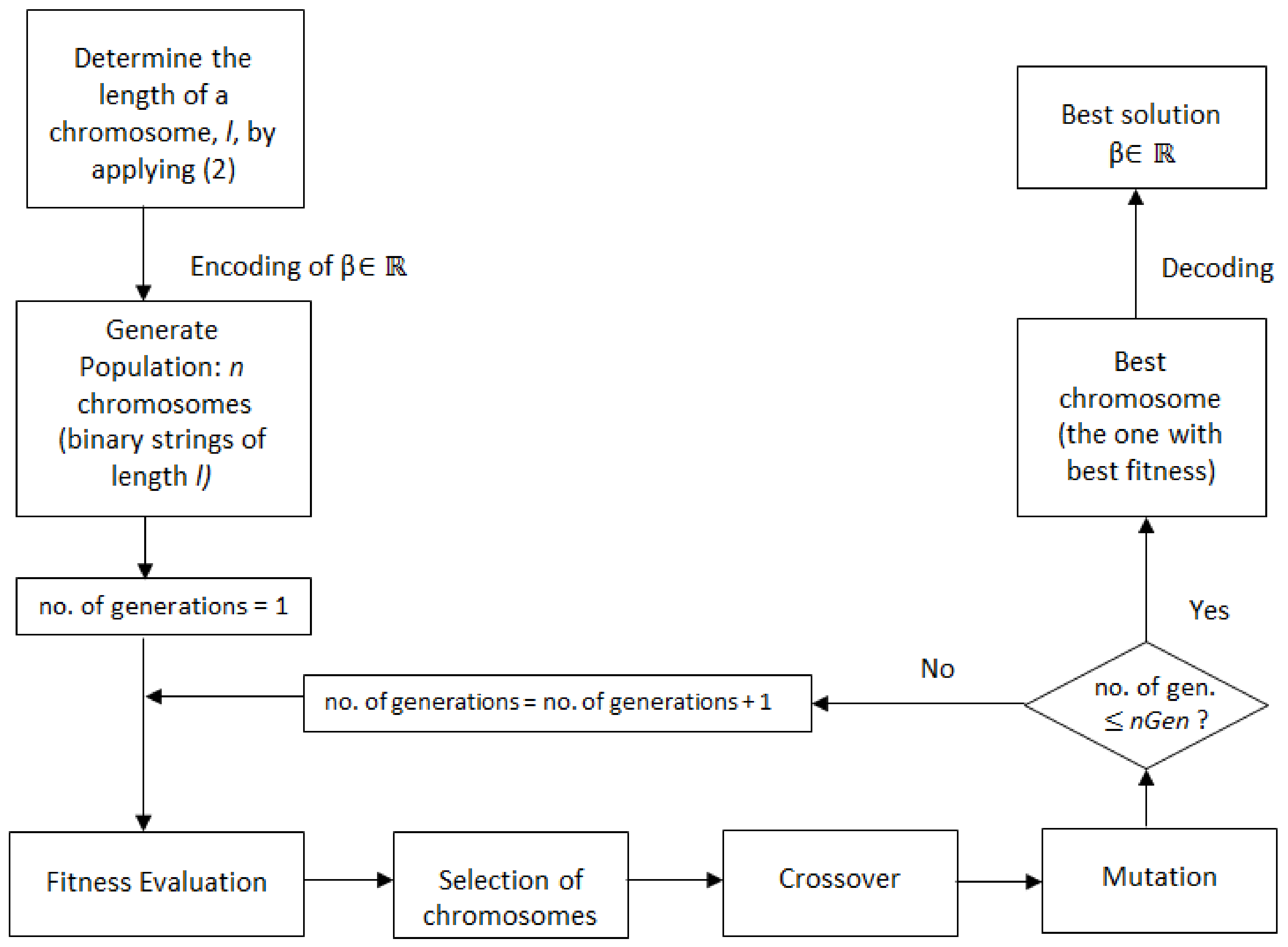
For a better understanding, a flowchart of the procedure of determination of the beta parameter is presented in Figure 1.
In order to find the best parameters settings for our problem, we fine tune our algorithm, which means creating several GA variants to test and find the best one, by slightly changing of GA parameters (population size, number of generations, crossover and mutation rates). We change only one parameter at a time, and try out several evolutionary literature-based test values. For example, for the crossover rate, the most used values in applications are in interval [0.6,1), whereas the mutation rate should be less than 10%. We run these GA variants on our problem, accept that parameter value at which the GA performs best, and continue to the next GA parameter, and so forth, to the last one. More precisely, to select the best population size, stop condition, and crossover rate the following steps are done.
- Step 1.
- We start with predefined values for the stop condition (10 generations), crossover rate (0.75), and mutation rate (0.015). Then, we vary the population size and compute the values of the fitness function. For each pair of operators (single-point/uniform, single-point/swap, two-point/uniform, two-point/swap), we chose the optimal population size to be the lowest value from which population growth does not significantly influence the modification of the fitness value.
- Step 2.
- With the population value determined at Step 1, the crossover rate, and the mutation rate kept at the same values as in Step 1, we run the algorithm to determine the best number of generations.
- Step 3.
- With the number of individuals determined at Step1, the number of generations determined at Step 2, and the mutation kept at the same value as in Step 1, we run the algorithm using different crossover rates, to determine the best crossover rate.
- Step 4.
- To find the best mutation rate, we set the best parameters from the previous steps and run the algorithm with different mutation rates.
- Step 5.
- The algorithm is run in each scenario with the new parameters determined in the previous steps.
Although the complexity of GAs has a probabilistic convergence time [30], the settings of our genetic algorithm are not complex, and, based on the experimental results that show that it converges in a short time, we may state that the best convergence time is logarithmic, O(log(n)), whereas the worst is linear, O(n). In the Results and Discussion, we present the recorded execution time (in seconds), which shows that the algorithms stop in short time for each test we did.
2.4. Data Series
Dobrogea is a region covering a surface between the Romanian Littoral of the Black Sea, the lower Danube River, and the Danube Delta, situated in the southeast part of Romania and characterized by long droughts periods. Records show the absence of precipitation for 4–6 months per year after 1961, which affects agricultural activities. Researchers analyzed precipitation and temperature evolution in this zone, especially after 2010, to mitigate the drought effects [31,32,33].
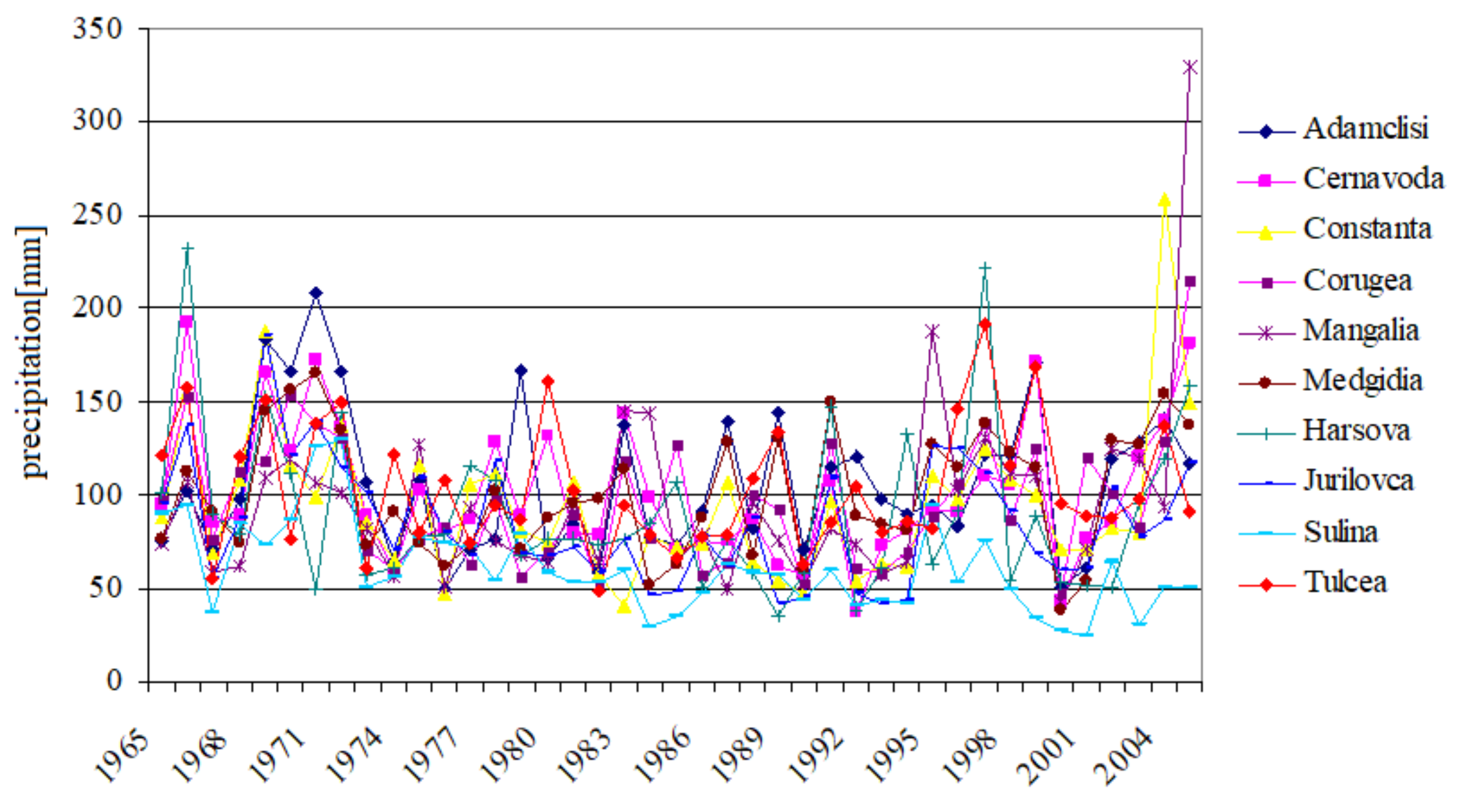
The data we are working with is formed by the maximum annual precipitation series recorded during a period of 41 years at 10 main meteorological stations from the Dobrogea region (Figure 2).
3. Results and Discussion
Firstly, we ran several tests to find the settings of control parameters that are most likely to produce the best results. We started with predefined values from the literature [27,28] for the stop condition (10 generations), crossover rate (0.75), and mutation rate (0.015). Then, we varied the population size (from 10 to 80, with a step of 5) and computed the fitness function’s corresponding values, run time, and β. Table 1 shows the relationship between the fitness value and population size.
For each pair of operators (single-point/uniform, single-point/swap, two-point/uniform, two-point/swap), we chose the optimal population size to be the lowest value from which population growth does not significantly influence the modification of the fitness value. This is 45, 40, 30, and 35 individuals, respectively, and the fitness function value is 0.0317. The corresponding β values obtained in the four scenarios are 1.256, 1.372, 1.308, and 1.336, respectively. These results are highlighted in Table 1.
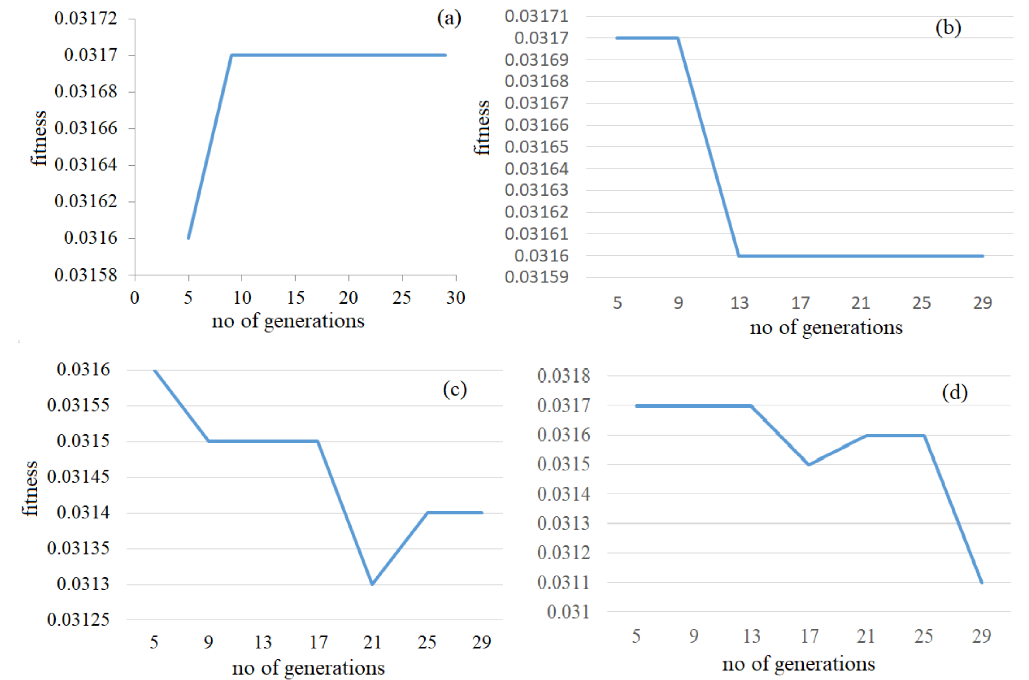
Since we used a predefined number of generations as the stop condition, in the second stage, we had to determine its optimal value. To find it, for each pair of operators, we ran tests with several values of the number of generations, the population size previously estimated (45, 40, 30, 35, respectively—Table 1), keeping the mutation rate set to 0.015, and the crossover rate set to 0.75. Table 2 and Figure 3 show that the fitness value does not improve after a certain number of generations (which is the optimal number of generations).
Based on the highest fitness value, the optimum number of generations determined was nine for the single-point/uniform mutation scenario, whereas, for the other scenarios, the number of generations was five. The corresponding β-values obtained are 1.228, 1.242, 1.122, and 1.362, respectively (highlighted in Table 2, together with the fitness and beta values). Since in our algorithm, β is represented by a chromosome, and several genetic operators have been used, different chromosomes (β) could produce the same fitness value.
The next step is the determination of the optimal crossover rate. For this aim, we ran the algorithm in each scenario with different values of the crossover rate (from 0.6 – value suggested in the literature to 0.95, with a step of 0.05), the population size and number of generations previously determined (45, 40, 30, and 35 individuals, respectively; 9, 5, 5, 5 generations, respectively), and the mutation rate kept to 0.015. We chose the optimal crossover rate for each pair of operators to be the value that gives the best (highest) fitness.
From Table 3 it results that the best crossover rates are 0.8 when using a single-point/uniform scenario, 0.6 for single-point/swap, 0.75 for two-point/uniform, and 0.7 for two-point/swap. These values correspond to the highlighted sequences of values in Table 3.
The last step was the determination of the best mutation rate. Therefore, we analyzed the impact the mutation rate has on the GA’s results. We considered the population size, the number of generations, and the crossover rates we established in previous stages, and we performed new tests aiming at detecting the value of the mutation rate. For example, for single-point uniform mutation, we took the population size = 45, the number of generations = 9, the crossover rate = 0.80, and ran the tests for a mutation rate from 0.02 to 0.1, with a step size of 0.01. For each pair of operators, we search the optimal mutation rate for which the fitness value evolves to a maximum along with the generations. Table 4 contains the values of the fitness function obtained after running the algorithm in the four scenarios, with different mutation rates. For example, in Table 4a we present the values of the fitness function obtained for each generation (from 1 to 9) and the mutation rates from 0.02 to 0.1, in the single-point crossover/uniform mutation scenario. The highest fitness value is obtained after nine generations in the single-point crossover/uniform mutation, with a mutation rate of 0.06 (the sixth column–the highlighted values).
In the single-point crossover/swap mutation (Table 4b), the highest fitness value is 0.0315, obtained after 5 generations, with a mutation rate of 0.08 (the eighth column of Table 4b). For the two-point crossover/uniform mutation and two-point crossover/swap mutation (Table 4c,d), the best mutation rates are 0.04 and 0.05, respectively, and the corresponding value of the fitness function is 0.0313 (contained in the highlighted columns—the fourth and the fifth, respectively).
After setting the optimal parameters, determined in the previous stages, we finally ran the algorithm to determine the optimum beta parameters. Table 5 summarizes the parameters used to implement the proposed genetic algorithm (columns 2–5), the fitness function obtained after running the algorithm with these parameters (column 6), the execution time (column 7), and the value obtained for the IDW’s parameter (last column).
Remark that the values of β are different when using different scenarios, even if the fitness value is the same. This is due to the specifics of the individuals’ selection and operations in GAs.
The lowest execution time (0.6188) is obtained when using the single-point/swap scenario and the highest one (10.5875 s) when using a two-point/swap procedure. Even if in the two-point/uniform case, the population size and the number of generations are the smallest, the execution time is high (the second-highest).
Table 6 contains the MSE and MAE for each station and the average (the last row of the table) computed after running the algorithm in each scenario. Comparing the MSEs in the two-point/swap and single-point/uniform (single-point/swap, and two-point/uniform) scenario, they are smaller in 70% (70%, 70%) cases, so our algorithm, in two-point/swap scenario, performs better in 70% cases compared to the other three scenarios. The MSEs’ averages (31.5874, 31.5306, 31.5188, 31.5153) are comparable, the smallest being obtained in the two-point/swap scenario, followed by the third one.
Comparing the MAEs in the two-point/swap and single-point/uniform (single-point/swap, and two-point/uniform) scenario, they are smaller in 80% (80%, 80%) cases, so our algorithm, in two-point/swap scenario, performs better in 80% cases compared to the other three scenarios. The MAEs’ averages (23.6352, 23.5542, 23.5308, 23.5228) are comparable, the smallest being obtained in the two-point/swap scenario, followed by the third one.
The corresponding values computed for beta in the best two cases are 1.042 (in two-point/swap) and 1.064 (in two-point/uniform).
For comparison reasons, we performed the classical IDW, with β = 2 (the value used in most applications) and β = 1.042. The MAE and MSE values computed for each station are presented in Table 7.
Comparing the MSEs in the two-point/swap algorithm (Table 6, column 8) with those from the IDW with β = 2 (Table 7 column 2), they are smaller in 70% cases (the first four stations, the sixth, eighth, and ninth), so our algorithm performs better in 70% cases. Comparing the MSEs in the two-point/swap algorithm with those from the IDW with β = 1.042 (Table 7 column 4), they are smaller in 60% cases (the second, third, fourth, sixth, eighth, and ninth stations), so our algorithm better performs in 60% cases.
In terms of the average MSEs, that in the two-point/swap approach is smaller than those of the IDW (β = 2), IDW (β = 1.042), and slightly higher than in KG (Table 7, the last column). Still, our approach is preferable against KG since it is difficult to determine the kriging parameters, requiring special knowledge of geostatistics.
The MAEs in the two-point/swap algorithm are smaller than those from the IDW with β = 2, in 80% cases (all, but the first and sixth station), and comparable for the first station.
The MAEs in the two-point/swap algorithm are smaller than those from the IDW (β = 1.042), they in 60% cases (all, but the first and sixth station), and comparable for the first station.
The average MAE in the two-point/swap approach (23.5228) is significantly smaller than those in the IDW with β = 2 (26.90), and IDW with β = 1.042 (26.08).
From the computational viewpoint, the highest computational time in our experiment was 10.5875 (in the two-point scenario), while in the grid search to estimate beta with 3 decimals takes 60 seconds for each series, so, a total of 60*10 stations = 600 seconds, which is 56.67 times higher than in our approach.
4. Conclusions
In this article, we presented a new approach to finding the beta parameter in IDW, using a GA implemented in four scenarios. The settings of this GA were optimized for finding the best fitness function and, by consequence, the best parameter beta, for all the study sites, not only for some of them.
It is shown that the algorithm proposed here performs better (in all scenarios) than the classical one (with β = 2 and β = 1.042) in terms of average MSE and MAE. When compared the MSEs and MAEs for the individual stations, the following results are obtained:
- In IDW with β = 2, MSE is smaller only for Hârșova, Mangalia, and Sulina, compared to the GA with a two-point swap.
- In IDW with β = 2, MAE is smaller only for Adamclisi and Mangalia, compared to the GA with a two-point swap.
- In IDW with β = 1.042, MSE is smaller than in GA (with two-point/swap) only for Adamclisi, Mangalia, and Sulina.
- In IDW with β = 1.042, MAE is smaller than in GA with a two-point swap only for Adamclisi, Cernavoda, and Mangalia.
The algorithm performs faster than the classical IDW, for which the running time on the same problem is 60s for each interpolated data series (so 600s for all ten series). It is easy to be implemented and used and can be applied to similar problems only by changing the input data.
Compared with other artificial intelligence methods used for finding beta (OIDW) our approach shows superior performances in 80% of cases.
Another advantage is that our algorithm provides a single beta for all the stations, optimizing the interpolation.
The results obtained in all four GA’s scenarios are comparable. Since the execution time is the highest in the best scenario (Table 5), the other alternatives can be successfully used for the spatial interpolation when the number of series or the number of records per station is very high.
Author Contributions
Conceptualization, A.B. and C.Ș.; methodology, A.B. and C.Ș.; software, C. Ș. and M.-L.I.; validation, A.B. and C.Ș.; writing—review and editing, A.B., C.Ș. and M.-L.I., visualization, C.Ș. and M.-L.I.; supervision, A.B. All authors have read and agreed to the published version of the manuscript.
Funding
This research received no external funding.
Conflicts of Interest
The authors declare no conflict of interest.
References
- Bărbulescu, A.; Popescu-Bodorin, N. History-based long-term predictability of regional monthly fuzzy data. Stoch. Environ. Res. Risk A 2019, 33, 1435–1441. [Google Scholar] [CrossRef]
- Li, J.; Heap, A.D. Spatial interpolation methods applied in the environmental sciences: A review. Environ. Modell. Softw. 2014, 53, 173–189. [Google Scholar] [CrossRef]
- Li, J.; Heap, A.D.; Potter, A.; Daniell, J.J. Application of machine learning methods to spatial interpolation of environmental variable. Environ. Modell. Softw. 2011, 26, 1647–1659. [Google Scholar] [CrossRef]
- Lu, G.Y.; Wong, D.W. An adaptive inverse-distance weighting spatial interpolation technique. Comput. Geosci. 2008, 34, 1044–1055. [Google Scholar] [CrossRef]
- Maleika, W. Inverse distance weighting method optimization in the process of digital terrain model creation based on data collected from a multibeam echosounder. Appl. Geomat. 2020, 12, 397–407. [Google Scholar] [CrossRef]
- Hsieh, H.H.; Cheng, S.J.; Liou, J.Y.; Chou, S.C.; Siao, B.R. Characterization of spatially distributed summer daily rainfall. J. Chin. Agr. Eng. 2006, 52, 47–55. [Google Scholar]
- Dirks, K.N.; Hay, J.E.; Stow, C.D.; Harris, D. High resolution studies of rainfall on Norfolk island part II: Interpolation of rainfall data. J. Hydrol. 1998, 208, 187–193. [Google Scholar] [CrossRef]
- Ly, S.; Charles, C.; Degré, A. Geostatistical interpolation of daily rainfall at catchment scale: The use of several variogram models in the Ourthe and Ambleve catchments, Belgium. Hydrol. Earth Sys. Sci. 2011, 15, 2259–2274. [Google Scholar] [CrossRef] [Green Version]
- Dong, X.H.; Bo, H.J.; Deng, X.; Su, J.; Wang, X. Rainfall spatial interpolation methods and their applications to Qingjiang river basin. J. China Three Gorges Univ. 2009, 31, 6–10. [Google Scholar]
- Bărbulescu, A. A new method for estimation the regional precipitation. Water Resour. Manag. 2016, 30, 33–42. [Google Scholar] [CrossRef]
- Chen, T.; Ren, L.; Yuan, F.; Yang, X.; Jiang, S.; Tang, T.; Zhang, L. Comparison of Spatial Interpolation Schemes for Rainfall Data and Application in Hydrological Modeling. Water 2017, 9, 342. [Google Scholar] [CrossRef] [Green Version]
- Golkhatmi, N.S.; Sanaeinejad, S.H.; Ghahraman, B.; Pazhand, H.R. Extended modified inverse distance method for interpolation rainfall. Int. J. Eng. Invent. 2012, 1, 57–65. [Google Scholar]
- Noori, M.J.; Hassan, H.; Mustafa, Y.T. Spatial estimation of rainfall distribution and its classification in Duhok governorate using GIS. J. Water. Resour. Protect. 2014, 6, 75–82. [Google Scholar] [CrossRef] [Green Version]
- Mei, G.; Xu, L.; Xu, N. Accelerating Adaptive IDW Interpolation Algorithm on a Single GPU. R. Soc. Open Sci. 2017, 4, 170436. [Google Scholar] [CrossRef] [PubMed] [Green Version]
- Gholipour, Y.; Shahbazi, M.M.; Behnia, A.R.A.S.H. An improved version of Inverse Distance Weighting metamodel assisted Harmony Search algorithm for truss design optimization. Latin Am. J. Solids Struct. 2013, 10, 283–300. [Google Scholar] [CrossRef] [Green Version]
- Zhang, X.; Liu, G.; Wang, H.; Li, X. Application of a hybrid interpolation method based on support vector machine in the precipitation spatial interpolation of basins. Water 2017, 9, 760. [Google Scholar] [CrossRef] [Green Version]
- Nourani, V.; Behfar, N.; Uzelaltinbulat, S.; Sadikoglu, F. Spatiotemporal precipitation modeling by artificial intelligence-based ensemble approach. Environ. Earth Sci. 2020, 79, 6. [Google Scholar] [CrossRef]
- Bărbulescu, A.; Băutu, A.; Băutu, E. Particle Swarm Optimization for the Inverse Distance Weighting Distance method. Appl. Sci. 2020, 10, 2054. [Google Scholar] [CrossRef] [Green Version]
- Chang, C.L.; Lo, S.L.; Yu, S.-L. The parameter optimization in the inverse distance method by genetic algorithm for estimating precipitation. Environ. Monit. Assess. 2006, 117, 145–155. [Google Scholar] [CrossRef]
- Ratnam, J.V.; Dijkstra, H.A.; Doi, T.; Morioka, Y.; Nonaka, M.; Behera, S.K. Improving seasonal forecasts of air temperature using a genetic algorithm. Sci. Rep. 2019, 9, 12781. [Google Scholar] [CrossRef] [Green Version]
- Nasseri, M.; Asghari, K.; Abedini, M.J. Optimized scenario for rainfall forecasting using genetic algorithm coupled with artificial neural network. Expert Syst. Appl. 2008, 35, 1415–1421. [Google Scholar] [CrossRef]
- Sen, Z.; Ôztopal, A. Genetic algorithms for the classification and prediction of precipitation occurrence. Hydrol. Sci. J. 2001, 46, 255–267. [Google Scholar] [CrossRef]
- Kadri, M.B.; Khan, W.A. Application of Genetic Algorithms in Nonlinear Heat Conduction Problems. Sci. World J. 2014, 2014, 451274. [Google Scholar] [CrossRef]
- Reddy, C.S.; Balaji, K. A Genetic Algorithm (GA)-PID Controller for Temperature Control in Shell and Tube Heat Exchanger. IOP Conf. Ser. Mater. Sci. Eng. 2020, 925, 012020. [Google Scholar] [CrossRef]
- Shepard, D. A Two-Dimensional Interpolation for Irregularly Spaced Data Function. In Proceedings of the 1968 ACM National Conference, New York, NY, USA, 27–29 August 1968; Blue, R.B., Rosenberg, A.M., Eds.; Association for Computing Machinery: New York, NY, USA, 1968; pp. 517–523. [Google Scholar]
- Lafitte, P. Traité d’Informatique Geologique; Masson: Paris, France, 1972. [Google Scholar]
- Sivanandam, S.N.; Deepa, S.N. Introduction to Genetic Algorithms; Springer: Berlin/Heidelberg, Germany, 2008. [Google Scholar]
- Haupt, R.L.; Haupt, S.E. Practical Genetic Algorithms; John Wiley & Sons Inc.: New York, NY, USA, 1998. [Google Scholar]
- Umbarkar, A.J.; Sheth, P.D. Crossover Operators in Genetic Algorithms: A Review. ICTACT J. Soft. Comp. 2015, 6, 1083–1092. [Google Scholar]
- Oliveto, P.S.; Witt, C. Improved time complexity analysis of the simple genetic algorithm. Theor. Comput. Sci. 2015, 605, 21–41. [Google Scholar] [CrossRef] [Green Version]
- Bărbulescu, A. Models for temperature evolution in Constanța area (Romania). Rom. J. Phys. 2016, 61, 676–686. [Google Scholar]
- Bărbulescu, A.; Deguenon, J. About the variations of precipitation and temperature evolution in the Romanian Black Sea Littoral. Rom. Rep. Phys. 2015, 67, 625–637. [Google Scholar]
- Bărbulescu, A.; Maftei, C.; Dumitriu, C.S. The modelling of the climateric process that participates at the sizing of an irrigation system. Bull. Appl. Comput. Math. 2002, 2048, 11–20. [Google Scholar]
Figure 1.
The procedure flow chart. nGen represents the maximum number of generations.

Figure 2.
Maximum annual precipitation series.

Figure 3.
The impact of the number of generations on fitness value in (a) single-point/uniform, (b) single-point/swap, (c) two point/uniform, (d) two point /swap scenarios.
Figure 3.
The impact of the number of generations on fitness value in (a) single-point/uniform, (b) single-point/swap, (c) two point/uniform, (d) two point /swap scenarios.


Table 1.
The impact of population size on the GA accuracy. The best results are highlighted.
| Scenario | Single Point/Uniform | Single Point/Swap | Two-Point/Uniform | Two-Point/Swap | ||||||||
|---|---|---|---|---|---|---|---|---|---|---|---|---|
| Pop. Size | Fitness | Time (s) | β | Fitness | Time (s) | β | Fitness | Time (s) | β | Fitness | Time (s) | β |
| 10 | 0.0311 | 0.300 | 2.528 | 0.0312 | 0.3156 | 2.316 | 0.0313 | 0.3500 | 2.186 | 0.0316 | 0.3625 | 1.580 |
| 15 | 0.0313 | 0.4625 | 1.500 | 0.0315 | 0.4688 | 1.612 | 0.0313 | 0.4719 | 2.154 | 0.0316 | 0.4781 | 1.568 |
| 20 | 0.0314 | 0.6062 | 1.862 | 0.0315 | 0.6031 | 1.742 | 0.0316 | 0.6375 | 1.514 | 0.0309 | 0.675 | 2.886 |
| 25 | 0.0315 | 0.8031 | 1.766 | 0.0315 | 0.8125 | 1.346 | 0.0315 | 0.7906 | 1.772 | 0.0313 | 0.7969 | 2.092 |
| 30 | 0.0316 | 0.9375 | 1.594 | 0.0315 | 0.9094 | 1.708 | 0.0317 | 0.9563 | 1.308 | 0.0315 | 0.9531 | 1.758 |
| 35 | 0.0316 | 1.0656 | 1.538 | 0.0316 | 1.0625 | 1.542 | 0.0317 | 1.1125 | 1.382 | 0.0317 | 1.100 | 1.336 |
| 40 | 0.0316 | 1.2813 | 1.494 | 0.0317 | 1.2188 | 1.372 | 0.0317 | 1.2813 | 1.298 | 0.0316 | 1.2437 | 1.620 |
| 45 | 0.0317 | 1.4312 | 1.256 | 0.0316 | 1.3687 | 1.382 | 0.0317 | 1.4094 | 1.208 | 0.0317 | 1.4781 | 1.212 |
| 50 | 0.0317 | 1.6781 | 1.480 | 0.0317 | 1.5781 | 1.128 | 0.0317 | 1.5375 | 1.308 | 0.0317 | 1.5594 | 1.274 |
| 55 | 0.0317 | 1.6906 | 1.324 | 0.0316 | 1.8375 | 1.552 | 0.0317 | 1.6938 | 1.132 | 0.0316 | 1.700 | 1.720 |
| 60 | 0.0317 | 1.8156 | 1.690 | 0.0317 | 1.850 | 1.258 | 0.0317 | 1.8750 | 1.122 | 0.0317 | 1.8469 | 1.192 |
| 65 | 0.0317 | 1.9625 | 1.212 | 0.0316 | 1.9781 | 1.510 | 0.0317 | 2.0156 | 1.294 | 0.0317 | 2.0938 | 1.246 |
| 70 | 0.0317 | 2.1781 | 1.248 | 0.0317 | 2.2062 | 1.056 | 0.0317 | 2.2250 | 1.200 | 0.0317 | 2.1656 | 1.210 |
| 75 | 0.0317 | 2.2437 | 1.306 | 0.0317 | 2.3062 | 1.126 | 0.0317 | 2.3406 | 1.262 | 0.0317 | 2.3687 | 1.282 |
| 80 | 0.0317 | 2.4406 | 1.162 | 0.0316 | 2.4469 | 1.382 | 0.0317 | 2.4500 | 1.320 | 0.0317 | 2.5844 | 1.306 |
Table 2.
The impact of the number of generations on the GA performance. The best results are highlighted.
Table 2.
The impact of the number of generations on the GA performance. The best results are highlighted.
| Scenario | Single Point/Uniform | Single Point/Swap | ||||||||
|---|---|---|---|---|---|---|---|---|---|---|
| Crossover Rate | Pop. Size | No. Gen | Fitness | Time (s) | β | Pop. Size | No. Gen | Fitness | Time (s) | β |
| 0.6 | 45 | 9 | 0.0316 | 1.2469 | 1.476 | 40 | 5 | 0.0317 | 0.6219 | 1.242 |
| 0.65 | 45 | 9 | 0.0316 | 1.2344 | 1.372 | 40 | 5 | 0.0317 | 0.6094 | 1.170 |
| 0.7 | 45 | 9 | 0.0316 | 1.2469 | 1.26 | 40 | 5 | 0.0317 | 0.6156 | 1.310 |
| 0.75 | 45 | 9 | 0.0316 | 1.2875 | 1.550 | 40 | 5 | 0.0317 | 0.6094 | 1.174 |
| 0.8 | 45 | 9 | 0.0317 | 1.2500 | 1.228 | 40 | 5 | 0.0317 | 0.6094 | 1.344 |
| 0.85 | 45 | 9 | 0.0317 | 1.2563 | 1.064 | 40 | 5 | 0.0317 | 0.6000 | 1.148 |
| 0.9 | 45 | 9 | 0.0317 | 1.2313 | 1.556 | 40 | 5 | 0.0316 | 0.6125 | 1.408 |
| 0.95 | 45 | 9 | 0.0317 | 1.2563 | 1.386 | 40 | 5 | 0.0316 | 0.6094 | 1.192 |
| Scenario | Two-Point/Uniform | Two-Point/Swap | ||||||||
| Cross Rate | Pop. Size | No. Gen | Fitness | Time (s) | β | Pop Size | No. Gen | Fitness | Time (s) | β |
| 0.6 | 30 | 5 | 0.0316 | 0.4594 | 1.424 | 35 | 5 | 0.0316 | 0.5625 | 1.538 |
| 0.65 | 30 | 5 | 0.0315 | 0.4750 | 1.964 | 35 | 5 | 0.0316 | 0.5594 | 1.578 |
| 0.7 | 30 | 5 | 0.0316 | 0.4719 | 1.564 | 35 | 5 | 0.0317 | 0.5344 | 1.362 |
| 0.75 | 30 | 5 | 0.0317 | 0.4594 | 1.122 | 35 | 5 | 0.0317 | 0.5313 | 1.252 |
| 0.8 | 30 | 5 | 0.0317 | 0.4562 | 1.532 | 35 | 5 | 0.0317 | 0.5375 | 1.208 |
| 0.85 | 30 | 5 | 0.0317 | 0.4688 | 1.400 | 35 | 5 | 0.0317 | 0.5313 | 1.348 |
| 0.9 | 30 | 5 | 0.0317 | 0.4688 | 1.326 | 35 | 5 | 0.0317 | 0.5469 | 1.124 |
| 0.95 | 30 | 5 | 0.0316 | 0.4531 | 1.406 | 35 | 5 | 0.0317 | 0.5469 | 1.274 |
Table 3.
The impact of crossover rate on the GA accuracy. The best results are highlighted.
| Scenario | Single-Point/Uniform | Single-Point/Swap | ||||||||
|---|---|---|---|---|---|---|---|---|---|---|
| Crossover Rate | Pop. Size | No. Gen | Fitness | Time (s) | β | Pop. Size | No. Gen | Fitness | Time (s) | β |
| 0.6 | 45 | 9 | 0.0316 | 1.2469 | 1.476 | 40 | 5 | 0.0317 | 0.6219 | 1.242 |
| 0.65 | 45 | 9 | 0.0316 | 1.2344 | 1.372 | 40 | 5 | 0.0317 | 0.6094 | 1.170 |
| 0.7 | 45 | 9 | 0.0316 | 1.2469 | 1.26 | 40 | 5 | 0.0317 | 0.6156 | 1.310 |
| 0.75 | 45 | 9 | 0.0316 | 1.2875 | 1.550 | 40 | 5 | 0.0317 | 0.6094 | 1.174 |
| 0.8 | 45 | 9 | 0.0317 | 1.2500 | 1.228 | 40 | 5 | 0.0317 | 0.6094 | 1.344 |
| 0.85 | 45 | 9 | 0.0317 | 1.2563 | 1.064 | 40 | 5 | 0.0317 | 0.6000 | 1.148 |
| 0.9 | 45 | 9 | 0.0317 | 1.2313 | 1.556 | 40 | 5 | 0.0316 | 0.6125 | 1.408 |
| 0.95 | 45 | 9 | 0.0317 | 1.2563 | 1.386 | 40 | 5 | 0.0316 | 0.6094 | 1.192 |
| Two-Point/Uniform | Two-Point/Swap | |||||||||
| Cross Rate | Pop. Size | No. Gen | Fitness | Time (s) | β | Pop Size | No. Gen | Fitness | Time (s) | β |
| 0.6 | 30 | 5 | 0.0316 | 0.4594 | 1.424 | 35 | 5 | 0.0316 | 0.5625 | 1.538 |
| 0.65 | 30 | 5 | 0.0315 | 0.4750 | 1.964 | 35 | 5 | 0.0316 | 0.5594 | 1.578 |
| 0.7 | 30 | 5 | 0.0316 | 0.4719 | 1.564 | 35 | 5 | 0.0317 | 0.5344 | 1.362 |
| 0.75 | 30 | 5 | 0.0317 | 0.4594 | 1.122 | 35 | 5 | 0.0317 | 0.5313 | 1.252 |
| 0.8 | 30 | 5 | 0.0317 | 0.4562 | 1.532 | 35 | 5 | 0.0317 | 0.5375 | 1.208 |
| 0.85 | 30 | 5 | 0.0317 | 0.4688 | 1.400 | 35 | 5 | 0.0317 | 0.5313 | 1.348 |
| 0.9 | 30 | 5 | 0.0317 | 0.4688 | 1.326 | 35 | 5 | 0.0317 | 0.5469 | 1.124 |
| 0.95 | 30 | 5 | 0.0316 | 0.4531 | 1.406 | 35 | 5 | 0.0317 | 0.5469 | 1.274 |
Table 4.
The impact of mutation rate on the GA accuracy. The best results are highlighted.
| a. Single-Point Crossover/Uniform Mutation | |||||||||
|---|---|---|---|---|---|---|---|---|---|
| Mutation Rate | |||||||||
| Gener. | 0.02 | 0.03 | 0.04 | 0.05 | 0.06 | 0.07 | 0.08 | 0.09 | 0.1 |
| 1 | 0.0307 | 0.0309 | 0.0309 | 0.0309 | 0.0308 | 0.0309 | 0.0310 | 0.0309 | 0.0309 |
| 2 | 0.0309 | 0.0310 | 0.0310 | 0.0310 | 0.0310 | 0.0309 | 0.0310 | 0.0310 | 0.0309 |
| 3 | 0.0309 | 0.0310 | 0.0310 | 0.0310 | 0.0310 | 0.0310 | 0.0311 | 0.0312 | 0.0309 |
| 4 | 0.0310 | 0.0311 | 0.0312 | 0.0310 | 0.0310 | 0.0311 | 0.0312 | 0.0312 | 0.0309 |
| 5 | 0.0310 | 0.0313 | 0.0312 | 0.0311 | 0.0312 | 0.0312 | 0.0312 | 0.0313 | 0.0309 |
| 6 | 0.0311 | 0.0313 | 0.0312 | 0.0311 | 0.0312 | 0.0312 | 0.0312 | 0.0313 | 0.0309 |
| 7 | 0.0311 | 0.0313 | 0.0313 | 0.0311 | 0.0312 | 0.0312 | 0.0312 | 0.0313 | 0.0309 |
| 8 | 0.0312 | 0.0313 | 0.0313 | 0.0311 | 0.0313 | 0.0312 | 0.0311 | 0.0312 | 0.0310 |
| 9 | 0.0313 | 0.0313 | 0.0313 | 0.0311 | 0.0314 | 0.0313 | 0.0311 | 0.0312 | 0.0312 |
| b. Single-Point Crossover/Swap Mutation | |||||||||
| Mutation Rate | |||||||||
| Gener. | 0.02 | 0.03 | 0.04 | 0.05 | 0.06 | 0.07 | 0.08 | 0.09 | 0.1 |
| 1 | 0.0308 | 0.0309 | 0.031 | 0.0309 | 0.0309 | 0.0309 | 0.0309 | 0.0308 | 0.0308 |
| 2 | 0.0308 | 0.0311 | 0.031 | 0.0309 | 0.0308 | 0.0309 | 0.0311 | 0.0311 | 0.0310 |
| 3 | 0.0308 | 0.0312 | 0.0312 | 0.0309 | 0.0308 | 0.031 | 0.0311 | 0.0311 | 0.0310 |
| 4 | 0.0309 | 0.0312 | 0.0312 | 0.031 | 0.0310 | 0.031 | 0.0312 | 0.0312 | 0.0311 |
| 5 | 0.0308 | 0.0313 | 0.0313 | 0.031 | 0.0310 | 0.0311 | 0.0315 | 0.0312 | 0.0311 |
| c. Two-Point Crossover/Uniform Mutation | |||||||||
| Mutation Rate | |||||||||
| Gener. | 0.02 | 0.03 | 0.04 | 0.05 | 0.06 | 0.07 | 0.08 | 0.09 | 0.1 |
| 1 | 0.0308 | 0.0308 | 0.0309 | 0.0308 | 0.0309 | 0.0311 | 0.0311 | 0.0308 | 0.0308 |
| 2 | 0.0309 | 0.0309 | 0.031 | 0.0309 | 0.0309 | 0.031 | 0.0313 | 0.0309 | 0.0309 |
| 3 | 0.0311 | 0.0309 | 0.0311 | 0.0311 | 0.0309 | 0.0311 | 0.0313 | 0.0311 | 0.0309 |
| 4 | 0.0311 | 0.0308 | 0.0312 | 0.0309 | 0.031 | 0.031 | 0.031 | 0.0311 | 0.0308 |
| 5 | 0.0311 | 0.0308 | 0.0313 | 0.0312 | 0.031 | 0.0312 | 0.0312 | 0.0311 | 0.0308 |
| d. Two-Point Crossover/Swap Mutation | |||||||||
| Gener. | 0.02 | 0.03 | 0.04 | 0.05 | 0.06 | 0.07 | 0.08 | 0.09 | 0.1 |
| 1 | 0.0308 | 0.0309 | 0.0311 | 0.0308 | 0.0308 | 0.031 | 0.0309 | 0.0309 | 0.0309 |
| 2 | 0.0309 | 0.031 | 0.0312 | 0.031 | 0.0311 | 0.031 | 0.031 | 0.031 | 0.0308 |
| 3 | 0.0308 | 0.031 | 0.0311 | 0.0312 | 0.0309 | 0.031 | 0.0311 | 0.031 | 0.0309 |
| 4 | 0.031 | 0.0311 | 0.0312 | 0.0313 | 0.0308 | 0.0309 | 0.0311 | 0.0312 | 0.0310 |
| 5 | 0.0311 | 0.031 | 0.0312 | 0.0313 | 0.0309 | 0.031 | 0.0311 | 0.0313 | 0.0309 |
Table 5.
The control parameters settings for the GA.
| Crossover/Mutation | Pop. Size | No. of Gen. | Crossover Rate | Mutation Rate | Fitness | Time (s) | β |
|---|---|---|---|---|---|---|---|
| Single-Point/Uniform | 45 | 9 | 0.8 | 0.06 | 0.0317 | 1.2437 | 1.318 |
| Single-Point/Swap | 40 | 5 | 0.6 | 0.08 | 0.0317 | 0.6188 | 1.124 |
| Two-Point/Uniform | 30 | 5 | 0.75 | 0.04 | 0.0317 | 7.5687 | 1.064 |
| Two-Point/Swap | 35 | 5 | 0.7 | 0.05 | 0.0317 | 10.5875 | 1.042 |
Table 6.
MSEs and MAEs in GA. The best results are highlighted.
| Station | Single-Point/Uniform | Single-Point/Swap | Two-Point/Uniform | Two-Point/Swap | ||||
|---|---|---|---|---|---|---|---|---|
| MSE | MAE | MSE | MAE | MSE | MAE | MSE | MAE | |
| Adamclisi | 36.2300 | 27.0536 | 36.1639 | 27.047 | 36.1372 | 27.0440 | 36.1264 | 27.0436 |
| Cernavoda | 22.9755 | 16.4861 | 22.7221 | 16.2628 | 22.6682 | 16.2290 | 22.6529 | 16.2254 |
| Constanta | 28.8453 | 17.0195 | 28.9273 | 17.2437 | 28.9601 | 17.3086 | 28.9731 | 17.3311 |
| Corugea | 21.0101 | 15.8130 | 21.0132 | 15.7836 | 21.0419 | 15.7770 | 21.0561 | 15.7744 |
| Harsova | 39.4587 | 26.2462 | 39.8004 | 26.2647 | 39.9151 | 26.2710 | 39.9581 | 26.2731 |
| Jurilovca | 24.5367 | 20.3591 | 24.4805 | 20.2806 | 24.4658 | 20.2606 | 24.4607 | 20.2534 |
| Mangalia | 36.4302 | 27.1703 | 36.3815 | 27.0490 | 36.3661 | 27.0040 | 36.3605 | 26.9864 |
| Medgidia | 26.8786 | 21.8044 | 26.5124 | 21.5704 | 26.3874 | 21.4822 | 26.3396 | 21.4471 |
| Tulcea | 33.5917 | 26.2378 | 33.5510 | 26.1170 | 33.5348 | 26.0791 | 33.5283 | 26.0667 |
| Sulina | 45.9171 | 38.1624 | 45.7538 | 37.9231 | 45.7115 | 37.8524 | 45.6972 | 37.8272 |
| Average | 31.5874 | 23.6352 | 31.5306 | 23.5542 | 31.5188 | 23.5308 | 31.5153 | 23.5228 |
Table 7.
MSE and MAE in the classical IDW for β = 2 and β = 1.042. MSE in ordinary kriging (KG).
| Station | IDW (β = 2) | IDW (β = 1.042) | KG * | OIDW ** | OIDW * | ||
|---|---|---|---|---|---|---|---|
| MSE | MAE | MSE | MAE | MSE | MSE | MSE | |
| Adamclisi | 36.32 | 27.03 | 35.73 | 26.96 | 32.73 | 32.4184 | 28.5774 |
| Cernavoda | 23.78 | 17.33 | 28.03 | 15.88 | 23.40 | 22.9189 | 22.6820 |
| Constanta | 37.29 | 27.80 | 35.83 | 27.09 | 30.22 | 30.3249 | 30.1713 |
| Corugea | 35.67 | 27.69 | 34.34 | 26.52 | 22.48 | 22.4062 | 22.3283 |
| Hârșova | 37.95 | 28.06 | 35.51 | 27.16 | 35.03 | 35.6281 | 35.2566 |
| Jurilovca | 34.89 | 27.89 | 34.35 | 27.31 | 23.04 | 24.1018 | 23.9813 |
| Mangalia | 35.65 | 26.86 | 35.03 | 26.81 | 42.73 | 42.0429 | 41.9517 |
| Medgidia | 35.89 | 27.41 | 34.89 | 26.82 | 22.58 | 22.3809 | 22.3073 |
| Tulcea | 38.55 | 29.84 | 36.15 | 28.19 | 43.54 | 44.0204 | 43.4118 |
| Sulina | 36.99 | 29.04 | 35.62 | 28.03 | 34.47 | 33.0844 | 33.0501 |
| Average | 35.30 | 26.90 | 34.55 | 26.08 | 31.02 | 30.93 | 30.37 |
Publisher’s Note: MDPI stays neutral with regard to jurisdictional claims in published maps and institutional affiliations. |
© 2021 by the authors. Licensee MDPI, Basel, Switzerland. This article is an open access article distributed under the terms and conditions of the Creative Commons Attribution (CC BY) license (http://creativecommons.org/licenses/by/4.0/).
Share and Cite
MDPI and ACS Style
Bărbulescu, A.; Șerban, C.; Indrecan, M.-L. Computing the Beta Parameter in IDW Interpolation by Using a Genetic Algorithm. Water 2021, 13, 863. https://doi.org/10.3390/w13060863
AMA Style
Bărbulescu A, Șerban C, Indrecan M-L. Computing the Beta Parameter in IDW Interpolation by Using a Genetic Algorithm. Water. 2021; 13(6):863. https://doi.org/10.3390/w13060863
Chicago/Turabian StyleBărbulescu, Alina, Cristina Șerban, and Marina-Larisa Indrecan. 2021. "Computing the Beta Parameter in IDW Interpolation by Using a Genetic Algorithm" Water 13, no. 6: 863. https://doi.org/10.3390/w13060863
Note that from the first issue of 2016, this journal uses article numbers instead of page numbers. See further details here.