Article

Detecting Climate Driven Changes in Chlorophyll-a in Deep Subalpine Lakes Using Long Term Satellite Data

1
Institute for Electromagnetic Sensing of the Environment, National Research Council, 20133 Milan, Italy
2
Department of Civil and Environmental Engineering, Politecnico di Milano, 20133 Milan, Italy
3
Water Research Institute, National Research Council, 28922 Verbania, Italy
*
Author to whom correspondence should be addressed.
Water 2021, 13(6), 866; https://doi.org/10.3390/w13060866
Submission received: 25 February 2021 / Revised: 17 March 2021 / Accepted: 19 March 2021 / Published: 23 March 2021

Abstract

:
Climate change has increased the temperature and altered the mixing regime of high-value lakes in the subalpine region of Northern Italy. Remote sensing of chlorophyll-a can help provide a time series to allow an assessment of the ecological implications of this. Non-parametric multiplicative regression (NPMR) was used to visualize and understand the changes that have occurred between 2003–2018 in Lakes Garda, Como, Iseo, and Maggiore. In all four deep subalpine lakes, there has been a disruption from a traditional pattern of a significant spring chlorophyll-a peak followed by a clear water phase and summer/autumn peaks. This was replaced after 2010–2012, with lower spring peaks and a tendency for annual maxima to occur in summer. There was a tendency for this switch to be interspersed by a two-year period of low chlorophyll-a. Variables that were significant in NPMR included time, air temperature, total phosphorus, winter temperature, and winter values for the North Atlantic Oscillation. The change from spring to summer chlorophyll-a maxima, relatively sudden in an ecological context, could be interpreted as a regime shift. The cause was probably cascading effects from increased winter temperatures, reduced winter mixing, and altered nutrient dynamics. Future trends will depend on climate change and inter-decadal climate drivers.

1. Introduction

Lakes are a useful medium through which to see the effects of climate change. Their nature as a semi-contained system, catchment, and lake basin with a distinct and fast-moving seasonal succession of flora and fauna, especially in plankton, marks them as rapidly responding ecosystems ideally suited to observe change. While the response may be complex resulting from interacting pressures, lake typology, and position on the trophic gradient, there is also significant value in interpreting an integrated signal to understand the impact on the natural environment [1,2].
Climate change is an important driver of global biodiversity in lakes and has been ranked third after invasive species and land-use change [3]. Projections suggest that climate change will have a much more widespread and substantial effect in the coming decades, altering land cover, hydrology, nutrient cycling, and species composition [4,5].
The global increase in summer surface temperature has been estimated as 0.34 °C decade−1, but the influence of local and lake-specific parameters such as morphology means that there is not often regional consistency to these trends [6]. In addition, many lakes in Europe now no longer cool to 4 °C, the maximum density of water. This critically affects a key mechanism, colder water sinking, by which deep lakes mix [7]. The ecological effects of climate change are complex, lake-specific, and often depend on multiple interacting pressures [8]. For example, phytoplankton can undergo changes to species composition, production, size structure, and phenology, which are likely to result in (and from) significant alteration to ecosystem functions at several trophic levels [2,9,10]. Higher temperatures in summer and more stable stratification has been predicted to lead to increased harmful algal blooms [11].
The deep subalpine lakes are of key economic importance in northern Italy, and their size and depth make them a key regional water resource requiring priority management [12,13]. A warming trend has been detected in the lakes, with annual average surface temperatures increasing 0.017 °C yr−1 and 0.032 °C yr−1 in summer [14]. This has led to more stable stratification in the lakes, increasing the isolation of the lower layers (hypolimnion) from the upper layers (epilimnion) with no complete mixing since 2006. This reduced mixing has led to a decreasing trend in oxygen concentrations in the hypolimnion, with the result that climate now exerts more control on oxygen than trophic status in these lakes [15]. This has also reduced nutrient transfer from the hypolimnion to the epilimnion as documented for Lake Garda, resulting in alterations to phytoplankton composition [16]. Generally, a process of oligotrophication of the epilimnion is occurring in the deep subalpine lakes while total phosphorous (TP) in the hypolimnion is increasing or remains stable [17]. Most studies have attributed the cause to long-term climate change and fluctuations in large-scale regional climate drivers such as the North Atlantic Oscillation (NAO) and especially the East Atlantic pattern (EA) during winter [15,16,17]. The implications of climate change in altering chlorophyll-a and phytoplankton groups have also been shown to be challenging to predict even with an eight-year calibration period at a monthly resolution for Lake Maggiore [18].
In this context, satellite remote sensing can enable the observation of a suite of functionally relevant indicators of water quality and ecosystem conditions for the study of long-term environmental trends in lakes [19]. A bibliometric analysis [20] has shown how optical remote sensing of lakes has expanded substantially over the past 50 years, with a sharp increase in the past 10–15 years as a consequence of improvements in sensor resolution. In this context, one of the most studied parameters is phytoplankton and, in particular, chlorophyll-a as a proxy of phytoplankton biomass. The spatial coverage and temporal sampling frequency achievable with satellite images absolutely provide novel insights into phytoplankton dynamic processes in lakes [21] that cannot be easily captured through in situ sampling [22,23]. In Europe, remote sensing has been identified as a key component of future implementation of the Water Framework Directive (WFD) that requires lakes are ecologically assessed using biological quality elements, including phytoplankton [24,25,26].
As regards the use of satellite observations of phytoplankton in subalpine lakes, several studies have been published since the mid-90s [27] for developing and testing algorithms to retrieve chlorophyll-a from space (e.g., Giardino et al. [28] and references in Odermatt et al. [29]), whether for assessing chlorophyll-a changes in single lakes [30] or for the entire subalpine lake district (e.g., Bresciani et al. [31] and reference therein). Specific studies have also been performed for assessing phytoplankton growth as a consequence of Saharan dust depositions [32], detecting cyanobacteria blooms [33,34], or to analyze phytoplankton dynamics in relation to lake surface water temperature [35,36].
Here, we examine a 16 year (2003–2018) time series for four deep subalpine lakes with the objective of identifying changes in chlorophyll-a in the context of climate change. Satellite observations of chlorophyll-a provide a higher temporal resolution that, in addition to their capacity to integrate signals over a large spatial area of the lake, allow a novel synoptic standardized picture to be leveraged to examine regional changes. We expect that the lack of deep mixing since 2005/2006 should be manifested in a disruption to the ecological functioning of the lake visible in altered chlorophyll-a seasonal patterns and concentration.

2. Materials and Methods
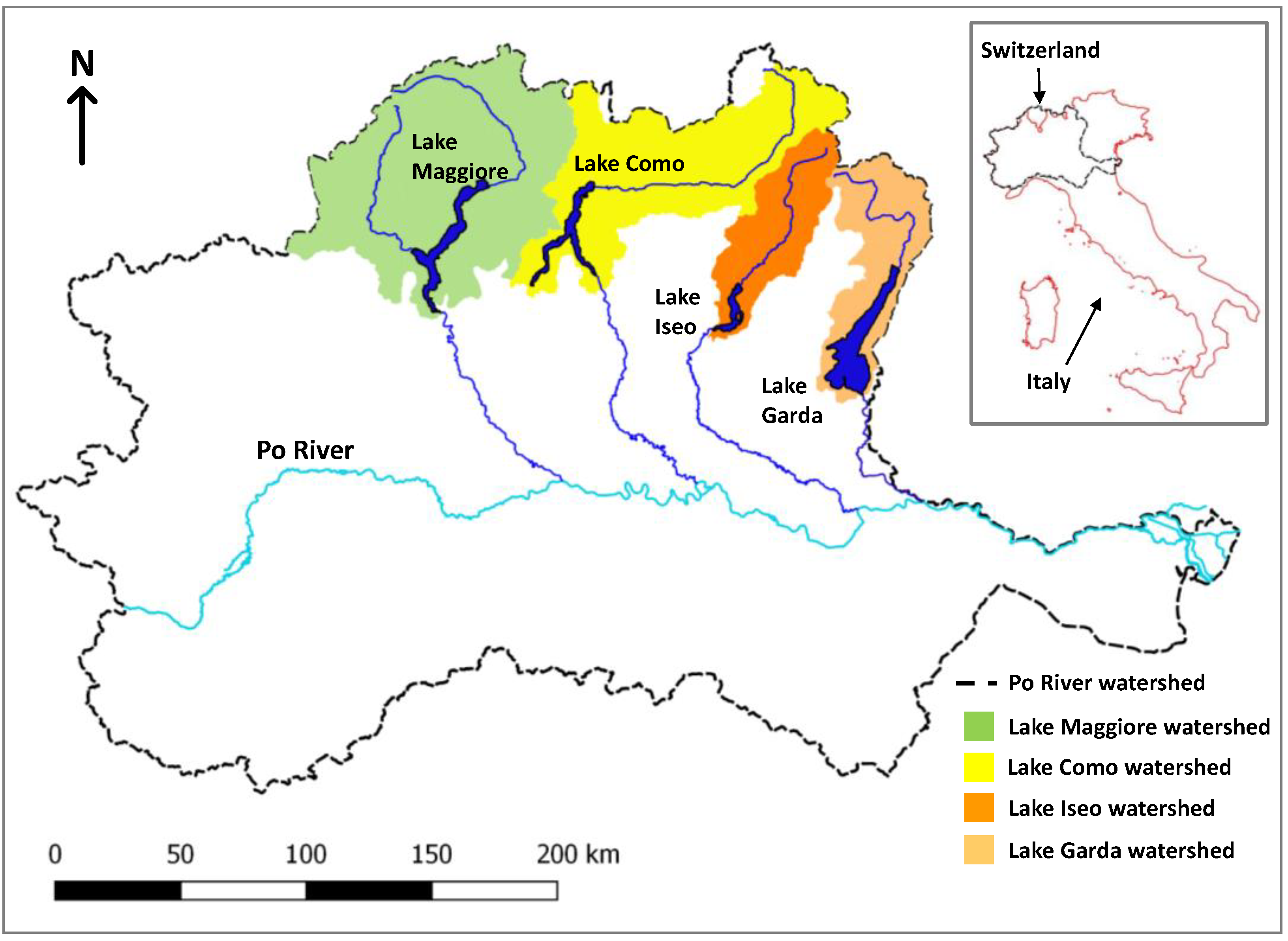
2.1. Study Sites

The 4 lakes are situated in the subalpine region of northern Italy and are all large (Figure 1, Garda: 368 km2, Como: 145 km2, Iseo: 61 km2, and Maggiore: 212 km2). Owing to climatic conditions and the deep maximum depth of the lakes (Garda: 350 m, Como: 410 m, Iseo: 258 m, and Maggiore: 370 m), mixing historically only occurred every 7 years, typically down to a depth of 200 m during cold and windy winters, while mixing in Iseo was prevented by a salinity gradient. The last deep mixing event was during 2005/2006 [15,16,37]. Total phosphorus trends have been analyzed for several depth aggregations from 1992–2016 [15]. Trends and recent (2016) concentrations were reported as increasing in Iseo (90 µg L−1) and Maggiore (13 µg L−1) and declining in Garda (18 µg L−1) and Como (35 µg L−1) for spring whole-column averages. However, the increases in Maggiore and Iseo were attributed to increasing hypolimnetic concentrations, whereas epilimnion (0–20 m) concentrations have been relatively stable after the 2005/2006 mixing event [15].

2.2. Collection and Processing of Satellite Data

The satellite measurements of chlorophyll-a concentrations used in this study were obtained from 4 optical sensors that allowed us to cover the temporal range 2003–2011 and 2014–2018. The older set of data were provided by MERIS (Medium Resolution Imaging Spectrometer) onboard of the Envisat-1 platform for 9 years and offered imagery data with a spatial resolution of 300 m. The more recent dataset was built with images acquired by optical sensors OLI (Operational Land Imager), MSI (multispectral instrument), and OLCI (Ocean and Land Colour Instrument), onboard Landsat-8, Sentinel-2, and Sentinel-3, respectively. The multispectral MSI sensor provided imagery data with a geometric resolution of 10 m to 60 m, the OLI sensor was 30 m, while the OLCI data offered a 300 m pixel resolution. Considering that the twin Sentinel-2 and Sentinel-3 satellites have been operational since 2015 (5 days revisit time) and 2017 (1–2 days revisit time), respectively, and adding the 16-day revisiting time of Landsat-8 as well as the fact that some lakes can be revisited twice due to the overlap of adjacent paths, there is at last an adequate replacement of MERIS, which had a 2–3 days revisit time.
For each sensor, satellite observation of chlorophyll-a data were obtained by processing cloud-free at-satellite-radiance data corrected for radiometric noise (e.g., atmospheric effects) to allow the computing of chlorophyll-a from atmospherically corrected images. In particular, for MERIS data, the processing was based on the method described in Odermatt et al. [29], which has been successfully adopted and validated in the study area [28,31]. In brief, radiometric noise was corrected using the BEAM-VISAT software (SMILE correction) [38], adjacency effects using the tool ‘Improved Contrast between Ocean and Land’ [39], and for simultaneously performing the correction of atmospheric effects and the retrieval of chlorophyll-a the ‘Case-2 Regional neural network processor’ was used [40,41].
In the case of newer OLI, MSI, and OLCI imagery, data have been processed using validated methods that were easily adaptable to the configurations (e.g., spectral setting) of the 3 sensors [34,42]. Briefly, the radiative transfer 6SV code [43] was used to first correct imagery data from atmospheric effects. Chlorophyll-a was then retrieved using the tool BOMBER [44], which implemented a bio-optical model that was parametrized with the specific inherent optical properties of subalpine lakes [34,45,46]. The consistency of results was further examined in this study by carrying out an ANOVA on the differences between field and satellite data, and no evidence was found for differences among the sensors (F = 0.3, p = 0.83, Figure S1).
For each chlorophyll-a product inferred from MERIS, OLI, MSI, and OLCI, regions of interest (ROI) were defined to extract the average value. The ROIs were defined to cover the equivalent surface area in units of km2 thus as to be not dependent on pixel size, which varied across the sensors. The ROIs positions are listed in Table 1 and a buffer of 1 km from the land was used to exclude the issues of shallow waters, mixed pixels, and residual noise for having miss-corrected adjacency effects.
The NAO and EA values were obtained from NOAA-CPC (https://www.cpc.ncep.noaa.gov/products/precip/CWlink/pna/nao.shtml (accessed on 2 April 2020)). Climatic data were obtained from ERA5—the 5th generation ECMWF reanalysis for the global climate and weather (monthly averaged data on single levels) (https://cds.climate.copernicus.eu/cdsapp#!/home (accessed on 15 January 2020)). Data used for analysis included: 10 m u-component of wind, 10 m v-component of wind, total precipitation, 2 m temperature (temperature of air at 2 m above the surface). The wind components were used to calculate wind speed and direction. The fraction of cloud cover and specific humidity were obtained from the ERA5 monthly averaged data on pressure level, with all data documentation available online: https://confluence.ecmwf.int/display/CKB/ERA5%3A+data+documentation (accessed on 15 January 2020). Total phosphorus data were obtained from regional authorities (ARPA Lombardia, ARPA Veneto) and published values [15,37]. Winter average values (DJF: December, January, February) were also calculated for NAO, EA, and air temperature as this has previously been found to be a key controlling parameter for these lakes [15,16,47]. The approach to analysis, primally based on satellite and climate data compiled and available at the global level should also ensure that the approach was scalable and portable to other areas, an important criterion for global change assessments.

2.3. Statistical Analysis

Nonparametric Multiplicative Regression (NPMR) [48] was used to estimate the response of average monthly chlorophyll-a to climate and environmental parameters listed above. NPMR can define response surfaces using predictors in a multiplicative rather than in an additive way. This method was progressive in better defining unimodal responses more typical of ecological data than other methods such as multiple regression [48]. It has previously been applied to model tree species distribution [49], the response of lichens to climate change [50], and in the time series analysis [51]. NPMR was applied using the software HyperNiche version 2.3 [52]. The response of chlorophyll-a was estimated using a local mean multiplicative smoothing function with Gaussian weighting. NPMR models were produced by adding predictors stepwise with fit expressed as a cross-validated R2 (xR2), which can be interpreted in a similar way as a measure of fit as a traditional R2. NPMR models were evaluated using a Monte Carlo procedure where concentration was randomized, the procedure rerun, and the proportion of models (p) (with the same number of predictors) with an xR2 greater than or equal to the original model evaluated. The sensitivity, a measure of the influence of each parameter included in the NPMR model, was estimated by altering the range of predictors by +/−0.05 (i.e., 5%) with resulting deviations scaled as a proportion of the observed range of the response variable. Therefore, a value of 1 would correspond to a change of equal magnitude in response and predictor variables. Sensitivity can be used to evaluate the relative importance of variables included in models because NPMR models are unlike linear regression and have no fixed coefficients or slopes. The order of inclusion of variables in the models was less important. Instead of fitting coefficients, in NPMR, tolerances were fit. These were reported in original units and represented one standard deviation of the smoothing function. Kendall’s tau test and the Theil-Sen slope for the significance and estimate of time series trends were carried out on environmental data in R [53]. Regression was performed in R [54].

3. Results

Chlorophyll-a in the four lakes showed significant variation over the 2003–2018 period (Figure 2). The temporal patterns could be considered as three phases. In the first phase up until 2010 (Como, Iseo) or 2012 (Garda, Maggiore) the seasonal pattern was typically defined by a significant bloom occurring during winter/spring (December-March) followed by a clear water phase and summer/autumn peaks. The second phase was defined by a period of low chlorophyll-a in Lakes Como and Iseo (2010–2011), Maggiore (2013–2014), and from 2014 an extended period of lower values in Garda. The third phase, comprising the remaining period up to 2018, had a seasonal pattern with less defined spring blooms and a tendency for annual maxima to occur in summer. The satellite data had gaps where no suitable images were available, including a large gap where the MERIS sensor satellite was not available in 2012. Nonetheless, the aforementioned transition in seasonal patterns was still visible, changing from essentially a concave to a convex annual pattern with more prominent mid-year concentrations.
In order to better understand the variation in chlorophyll-a over time, we carried out a non-parametric multiplicative regression analysis on each of the lakes (Table 2). The models for all four lakes were significant, with xR2 ranging from 0.49 to 0.64. Time and air temperature were consistently included in models for all four lakes. Variables averaged over the winter period were also included in the models for all lakes: Temperature (Garda) and DJF NAO (Maggiore, Iseo, Como, Italy). The concentration of total phosphorus was also included in the model for Lake Iseo. The sensitivity value provided an indication of the importance of the variables in the models. In Lake Garda, winter temperature had the highest sensitivity value (0.31), and in Iseo and Como the monthly temperature had the highest sensitivity (0.23 and 0.27, respectively). In Maggiore, the time variable had the highest sensitivity (0.54). Monthly temperature sensitivity values ranged from 0.23–0.27 among the four lakes.
Contour plots were produced to visualize model results for chlorophyll-a with temperature over time (Figure 3). The contour lines and color intensity represent chlorophyll-a in 1 µg L−1 increments. Common to all the lakes were the higher concentrations in the bottom left of the figures occurring at lower temperatures (<10 °C) typically found over the winter-spring during the period 2003–2010. Directly above this, in the upper left, were lower concentrations typically found at higher summer temperatures during this period. This pattern then appeared to change. For Lakes Como and Maggiore, from about 2010 or 2013, the pattern was inverted, with higher concentrations now being found at higher temperatures (summer) and lower concentrations at lower temperatures in the winter-spring. Garda and Iseo appeared to transition to lower concentrations with more uniform concentrations at all temperatures.
The directional influence of the other variables was examined through additional NPMR response plots (see Supplementary Materials). In Lake Maggiore, only a minor influence of the climate index DJF NAO was indicated by the low sensitivity value (0.02, Table 2), and this is visible in the response plot showing only a very marginal increase in chlorophyll-a at more negative values of the DJF NAO (Figure S2). In Lake Como, positive values of the DJF NAO were associated with higher estimated chlorophyll-a concentrations up until about 2011, when the reverse was true with more negative values leading to higher chlorophyll-a (Figure S3). Similarly, in Iseo, positive values of the DJF NAO were associated with higher estimated chlorophyll-a concentrations, the influence of which declined from 2009 (Figure S4). Total phosphorus was also included in the model for Iseo and was predicted to increase chlorophyll-a concentrations as would be expected (Figure S5). In Lake Garda higher chlorophyll-a was associated with lower DJF air temperatures (Figure S5). It is interesting that the EA index was not included in the models rather that the NAO—this may be because of its relationship with temperature—which was already selected for model inclusion. For example, winter air temperature was positively correlated with winter EA for Como (rS = 0.82, p < 0.01), Iseo (rS = 0.69, p < 0.01) and Garda (rS = 0.58, p = 0.02) but not Maggiore (rS = 0.42, p = 0.11), where it was more correlated with the NAO (rS = 0.68, p < 0.01).
As mentioned above, the seasonal pattern centred around summer appeared to undergo a shift from a concave to a convex pattern (Figure 2). In order to examine this shift in the seasonal pattern in more detail, we fitted a second-order polynomial to chlorophyll-a each year between April and October. The coefficient of the squared term was then assessed to see if it was changing from positive (indicating a concave curve) to negative (indicating a convex curve) over time. A significant negative trend was found for Lakes Como, Iseo (p ≤ 0.002), and Garda (p ≤ 0.05) but not for Maggiore (p = 0.08) (Figure 4).
To indicate environmental change over time that may be contributing to the disruption and alteration of chlorophyll-a concentrations, we tested trends in a longer dataset (1980–2018) for the four lakes (Table 3). Trends in air temperature for all four lakes were highly significant, with slopes ranging from 0.062 to 0.069. Similarly, DFJ air temperature slopes ranged from 0.049 to 0.073. The total increase in annual average ranged from 2.3 to 2.6 °C over the 39 years. Rainfall and wind speed did not show a significant difference in annual averages with the exception of Lake Iseo, which had a slight decline in wind speed (Table 3).

4. Discussion

The dataset covered four lakes across the Italian-Swiss subalpine region of differing trophic conditions. Examination of the dataset and NPMR model contour plots indicated that there had been a disruption to the pre-2010 pattern of well-defined spring peak, clear water phases followed by summer peaks. Following a one or two-year period of low chlorophyll-a (which extended for Lake Garda), the seasonal pattern had less defined spring blooms and a tendency for annual maxima to occur in summer. Contour plots from the NPMR analysis indicated that this pattern of shifting spring to summer maxima was similar for Como and Maggiore, while Garda and Iseo had less pronounced spring chlorophyll-a over time. The consistency of this pattern of change suggests a regional controlling influence such as climate rather than catchment-specific factors.
All of the NPMR models included a winter climatic parameter (DJF NAO or winter air temperature), indicating the importance of regional climate patterns in controlling chlorophyll-a. In Lake Garda, colder winter temperatures were found to increase the chlorophyll-a concentration, and its importance was underlined by it being the most sensitive parameter included in the NPMR model. In Lake Como, the influence of the DJF NAO appeared to change from 2011 with more negative values leading to higher chlorophyll-a. Similarly, in Lake Maggiore, concentrations were predicted to be higher at more negative DJF NAO from 2011 but only marginally so. In contrast, in Lake Iseo, more positive values of the NAO consistently led to higher chlorophyll-a. Although EA was not directly included in any of the models, a more negative EA is known to be associated with colder air temperatures [16] and a significant correlation with winter temperature was found for Lakes Como, Iseo, and Garda in this dataset. As temperature was preferentially selected by the models, EA may not have explained residual variation and, therefore, would not be included in models. Further evidence for a change in chlorophyll-a pattern was evident in a shift from a concave to a convex seasonal pattern centered around summer visible in the plotted time series. This was examined using the coefficient of the squared term of the second-order polynomial. The lakes had a significant trend in the coefficient, reflecting a shift from a concave to a convex pattern between April to October with the exception of Lake Maggiore. Interestingly a steeper slope and higher r2 were observed for more eutrophic lakes such as Iseo and Como compared to Garda and Maggiore, indicating that nutrient concentrations may condition the change in seasonal pattern. However, it is recommended to test this observation by conducting a wider application of this method to other deep lakes undergoing alteration to stratification across a nutrient gradient.
The destabilization of stratification with lower surface water temperatures and sinking of colder water in winter is one of the principal mechanisms contributing to deep lake mixing [7,55], and positive values in the EA and NAO, resulting in higher winter temperatures that are likely to critically alter this process. The winter EA has been found to be increasing since the 1950s [16]. A recent analysis on 635 lakes worldwide has predicted that for 100 lakes, their mixing regimes are likely to be altered under climate change scenarios, with some at risk of becoming permanently stratified, reducing nutrient upwelling, and decreasing hypolimnion oxygen [56]. This may be the situation for this set of subalpine lakes as positive values in the EA and NAO, and higher winter temperatures have been linked to a shallower mixing depth and the failure of the subalpine lakes to fully mix since 2005/2006 [15]. The observed decline in spring chlorophyll-a and alteration of the seasonal pattern is, therefore, likely a response to lower transport of nutrients to the epilimnion and the altered physical structure imposed by climate-driven changes to the stratification regime. The large-scale warming in the northern hemisphere since the 1970s has been attributed to anthropogenic radiative forcing and also to the multidecadal pattern of the North Atlantic Oscillation (NAO), which had a positive phase from the 1980s to the early 2000s, resulting in poleward heat transport [57]. However, the next decade may see a more negative phase with lower temperatures [57], and this could increase the likelihood of a full overturn in these lakes, which, in some cases, would transport substantial amounts of nutrients, given their accumulation in the hypolimnion, and radically alter the phytoplankton dynamics [15,16].
Total phosphorus concentration was significant in the NPMR for Iseo, and this lake had relatively the highest concentrations over the examined time period (Rogora et al., 2018). Previous analysis found that these subalpine lakes had broadly stable epilimnion TP concentrations over the period (Rogora et al., 2018) and this is probably a contributing factor as to why the influence of climate on chlorophyll-a was detectable. Given the strong deterministic effect of phosphorus in controlling algal populations [58], it is likely that in many other lakes globally, the variation in nutrients will obscure the influence of climate change on chlorophyll-a. While rainfall was not included directly in any of the NPMR models, the increasing frequency of extreme rainfall events has been linked to transporting nutrients to Lake Maggiore supporting summer blooms of cyanobacteria that have occurred regularly since 2005 [59]. Wind speed was not included in the NPMR for the lakes.
The observation of a period of disruption to the cycle of one to two years is interesting. It may represent a lag phase when the phytoplankton community is adjusting to changed environmental conditions resulting from reducing water column mixing. Although given the significant diversity in the phytoplankton and the persistence, at least at a low density of many species, it would be unusual that some species would not respond quicker [60]. In addition, in the ocean, reduced mixing has been found to lead to oscillations and disruption to phytoplankton through increasing loss of nutrients via sinking phytoplankton coupled with less upward movement of nutrients from lower layers [61]. However, the reduction in production driven by ocean stratification [62] was not, in purely proportional terms, as notable as the drop observed here. Further work is needed to examine the changes in species composition and drivers behind this period of low chlorophyll-a in order to understand if there are lessons on the implications of climate change for other ecosystems. In Lake Garda, the chlorophyll-a continued to be consistently lower after 2012, the reasons for which are uncertain but could be related to the fact that the temperature is consistently 1 to 2 °C higher in this lake compared to the others [15], which could strengthen the stratification further inhibiting nutrient transfer to the epilimnion.
The increase in temperature with climate change, mediated by the NAO, has led to an earlier occurrence of the spring diatom bloom in Sweden based on March NAO values (Weyhenmeyer et al., 1999). While the key climatic driver of warmer temperatures leading to earlier spring bloom may be clear, the implications posed by the absence of winter mixing may be more complex. It is expected that the species composition and abundance of the phytoplankton are likely to be altered and undergo disruption to the established seasonal succession of species. Ordinated long time series of phytoplankton community composition have shown shifts from being associated with euphotic depth and nutrient ratios in the 1980s to stratification strength and thermocline depth in the 1990s [63]. Moreover, while blooms of cyanobacteria are notably favored by increasing water temperature and column stratification in nutrient-rich lakes, blooms of different phytoplankton groups or taxa may occur in oligotrophic conditions at analogous physical conditions of high water column stability. Mougeotia, a filamentous green phytoplankton species that competes well at lower nutrient levels [64,65] and stratified conditions, recorded mass developments during recent decades in some large subalpine lakes such as Lakes Geneva, Garda, and Maggiore [66]. In particular, it was observed to dominate at over 80% of total phytoplankton biomass during the summer of 2011 in Lake Maggiore, the highest value in records dating from 1984. Filamentous green algae, smaller diatoms, cyanobacteria, and other species capable of depth regulation are favored with intensified stratification [63]. Similarly, in Lake Garda, the increased stratification resulted in lower epilimnion nutrients and was found to lead to a shift to motile species such as dinoflagellates and cryptophytes as well as changes in the cyanophyte community [16]. Alteration of the phytoplankton community, development timing and magnitude of seasonal peaks in chlorophyll-a can have cascading effects on the ecosystem, impacting zooplankton and higher trophic levels such as fish [10]. Further investigation at high temporal resolution is needed on summer nutrient and plankton dynamics to understand the increased chlorophyll-a concentrations better.
Climate change can have a significant influence on lakes through indirect and unanticipated pathways. This study found reduced winter turnover likely exerted significant control reducing the concentration of chlorophyll-a but also considerably altered the seasonal pattern. At higher latitudes, an increase in the length of the growing season has been attributed not to a direct influence of higher temperatures but rather to an increasing proportion of rain relative to snow resulting in earlier delivery of the nutrient load to lakes [67]. While climate change may have direct physiological consequences associated with higher temperature, often the effects of the change on the structural functioning of the catchment and lake can have more powerful effects [11]. The restructuring of ecosystems is likely to be of more important than individual species temperature thresholds and difficult to anticipate.
Satellite observations may have proved essential in revealing these trends in chlorophyll-a concentration over time. The benefits of using remote sensing to assess chlorophyll-a are the good spatial, temporal, and synoptic ability allowing several lakes to be assessed in a consistent approach [28]. While data gaps are a feature of the satellite record, the principal pattern of a switch from a concave shape (spring peak, clear phase, and summer/autumn peak) to a convex shape (dominant summer concentrations) was visible from the satellite record alone. This is important to demonstrate as the approach could be used to examine alterations in plankton dynamics from climate change in unmonitored lakes globally. However, it would be important to account for differing optical lake types to ensure a better relationship between reflectance and chlorophyll-a [68]. Opportunities to extend such approaches have recently been advanced with the European Space Agency’s commitment to providing data on climate variables for lakes, including chlorophyll-a [69]. An important drawback of using remote sensing is the satellite’s inability to provide a depth profile of chlorophyll-a, with satellite estimates being dependent on light penetration equating to 90% of Secchi depth [70]. Chlorophyll-a is well known to vary significantly with depth—often having a maxima below 10 m with particular species adapted to live even deeper [71,72]. This may be important given the switch to more motile species such as dinoflagellates and cryptophytes as in Lake Garda [16]. It is possible that the lower surface chlorophyll-a in Lake Garda recorded by satellite could be an artifact and reflect a shift to motile species occurring at a deeper depth.
Ideally, a high-resolution dataset covering temporal, spatial, and depth gradients would be available to allow a comprehensive analysis. Several observations can be gathered per month by satellites, often during the summer period when cyanobacterial blooms occur, thereby defining these events more adequately than a fixed field schedule could afford [73]. However, cloud cover often means that one or more months may not have adequate data. An alternative approach could incorporate in situ or modeled data, although as field data are often depth-integrated, this could be challenging. Some approaches have aggregated many years of data to define seasonal patterns, such as 10-year sliding windows [67].
In Europe, the Water Framework Directive (WFD) requires that lakes are ecologically assessed using biological quality elements, including phytoplankton (chlorophyll-a as well as taxonomic composition). Ecological status is measured as deviation from reference condition, which varies depending on lake type and geographic region [22,23,74]. The system adopted for alpine lakes included only altitude, mean depth, alkalinity, and lake size [75]. However, the mixing characteristics of the lake were included as optional type parameters in the directive [22]. Climate change may, therefore, create pressure to alter management targets and strategies as the lake typology and, therefore, ecological status boundaries may effectively change, presenting a management dilemma between unobtainable goals and the need to protect and improve water quality [4]. While chlorophyll-a may decline with continued stratification, superficially indicating an improvement, other biological quality elements such as macroinvertebrates in the sub-littoral and profundal zones may deteriorate given the lower oxygen concentrations below the thermocline [76]. Climate change may, therefore, test whether the intentions of the WFD to appraise the structure and functioning of freshwater ecosystems can be realized given current approaches.
Answering the question as to whether a tipping point has been passed, leading to a regime shift and alternative state for the subalpine lakes, can risk being caught in semantics. A strict interpretation of a tipping point is one past which a previous ecological state cannot be regained, an irreversible change [77]. Obviously, the permanency of this depends on future climatic trends. However, frequent past anomalies in the mixing behavior of lakes are likely a predictor of future regime shift with climate change [56].

5. Conclusions

A significant change in the seasonal pattern of chlorophyll-a occurred in the four subalpine lakes under study between 2003–2018. There was a shift from a dominant spring peak, clear water phase, and summer peak to a weakened spring peak with more prominent summer concentrations. Non-parametric multiplicative regression indicated that winter climatic variables were important, with higher values of the NAO and higher temperatures likely reducing the amount of thermal mixing in the lakes. The key driver is, therefore, likely to be higher winter temperatures linked to the failure since 2005/2006 of the lakes to mix fully, resulting in lower nutrient concentrations in the epilimnion. The satellite estimation of chlorophyll-a and its capacity to gather a regional synoptic picture may have proved essential in revealing the changing trend over this 16 year period. The permanency of this significant change to the subalpine lakes will depend on climate change and inter-decadal climate drivers.

Supplementary Materials

The following are available online at https://www.mdpi.com/2073-4441/13/6/866/s1, Figure S1: Boxplot showing the difference from mean chlorophyll-a among sensors used. No evidence was found for a difference among sensors (ANOVA, F = 0.96, p = 0.42, n = 5.5). Differences were based on chlorophyll-a determined in-situ (within a 3-day timeframe) and that estimated using the sensors aboard the different satellites used in this study. Figure S2: Lake Maggiore response curves for chlorophyll-a (μg L−1) with DJF NAO. Figure S3: Lake Como response curves for chlorophyll-a (μg L−1) with DJF NAO. Figure S4: Lake Iseo response curves for chlorophyll-a (μg L−1) with DJF_EA and TP. Figure S5: Lake Garda response curves for chlorophyll-a (μg L−1) with DJF Temperature °C.

Author Contributions

Conceptualization, M.B., G.F., M.P. and C.G.; data curation, M.B., M.P., G.F., N.G. and G.L.; formal analysis G.F.; methodology, M.B., G.F. and C.G.; supervision, C.G.; validation, M.B., N.G., G.L. and C.G.; writing—original draft, G.F., M.B., M.P., R.C.; writing—review and editing, M.B., M.P., N.G., G.L., R.C. and C.G. All authors have read and agreed to the published version of the manuscript.

Funding

Part of the satellite processing activities was included in the FP7 GLaSS project (GA n. 313256) and H2020 EOMORES project (GA n. 730066), and in the Interreg Italy/Swiss SIMILE Project. Funding for data analysis was supported by the ESA CCI LAKES project (GA n. 40000125030/18/I-NB).

Institutional Review Board Statement

Not applicable.

Informed Consent Statement

Not applicable.

Data Availability Statement

The datasets generated during and/or analyzed during the current study are available from the corresponding author on reasonable request.

Acknowledgments

We thank ARPA Lombardia and ARPA Veneto for the provision of environmental data. In situ chlorophyll-a data for Lake Maggiore were collected through the limnological campaigns funded by the International Commission for the Protection of Waters between Italy and Switzerland (CIPAIS). We thank Giacomo Foppiano for assistance with data collation. We are very grateful to four anonymous reviewers for the valuable comments and suggestions that helped improve this study.

Conflicts of Interest

The authors declare no conflict of interest.

References

  1. Adrian, R.; O’Reilly, C.M.; Zagarese, H.; Baines, S.B.; Hessen, D.O.; Keller, W.; Livingstone, D.M.; Sommaruga, R.; Straile, D.; van Donk, E.; et al. Lakes as sentinels of climate change. Limnol. Oceanogr. 2009, 54, 2283–2297. [Google Scholar] [CrossRef] [PubMed]
  2. Weyhenmeyer, G.A.; Blenckner, T.; Pettersson, K. Changes of the plankton spring outburst related to the North Atlantic oscillation. Limnol. Oceanogr. 1999, 44, 1788–1792. [Google Scholar] [CrossRef] [Green Version]
  3. Sala, O.E.; Chapin, F.S., III; Armesto, J.J.; Berlow, E.; Bloomfield, J.; Dirzo, R.; Huber-Sanwald, E.; Huenneke, L.F.; Jackson, R.B. Global biodiversity scenarios for the year 2100. Science 2000, 287, 1770. [Google Scholar] [CrossRef] [PubMed]
  4. Cardoso, A.C.; Free, G.; Nõges, P.; Kaste, Ø.; Poikane, S.; Solheim, A.L. Lake management, criteria. In Encyclopedia of Inland Waters; Likens, G.E., Ed.; Academic Press: Cambridge, MA, USA, 2009; pp. 310–331. ISBN 978-0-12-370626-3. [Google Scholar]
  5. Carpenter, S.R.; Stanley, E.H.; Vander Zanden, M.J. State of the world’s freshwater ecosystems: Physical, chemical, and biological changes. Annu. Rev. Environ. Resour. 2011, 36, 75–99. [Google Scholar] [CrossRef] [Green Version]
  6. O’Reilly, C.M.; Sharma, S.; Gray, D.K.; Hampton, S.E.; Read, J.S.; Rowley, R.J.; Schneider, P.; Lenters, J.D.; McIntyre, P.B.; Kraemer, B.M.; et al. Rapid and highly variable warming of lake surface waters around the globe. Geophys. Res. Lett. 2015, 42, 10773–10781. [Google Scholar] [CrossRef] [Green Version]
  7. Woolway, R.I.; Weyhenmeyer, G.A.; Schmid, M.; Dokulil, M.T.; de Eyto, E.; Maberly, S.C.; May, L.; Merchant, C.J. Substantial increase in minimum lake surface temperatures under climate change. Clim. Chang. 2019, 155, 81–94. [Google Scholar] [CrossRef] [Green Version]
  8. Craig, L.S.; Olden, J.D.; Arthington, A.H.; Entrekin, S.; Hawkins, C.P.; Kelly, J.J.; Kennedy, T.A.; Maitland, B.M.; Rosi, E.J.; Roy, A.H. Meeting the challenge of interacting threats in freshwater ecosystems: A call to scientists and managers. Elem. Sci. Anth. 2017, 5, 1–15. [Google Scholar] [CrossRef]
  9. Jeppesen, E.; Meerhoff, M.; Davidson, T.A.; Trolle, D.; Lauridsen, T.L.; Beklioglu, M.; Brucet, S.; Volta, P.; Gonzalez-Bergonzoni, I.; Nielsen, A. Climate change impacts on lakes: An integrated ecological perspective based on a multi-faceted approach, with special focus on shallow lakes. J. Limnol. 2014, 73, 88–111. [Google Scholar] [CrossRef] [Green Version]
  10. Winder, M.; Sommer, U. Phytoplankton response to a changing climate. Hydrobiologia 2012, 698, 5–16. [Google Scholar] [CrossRef]
  11. O’Neil, J.M.; Davis, T.W.; Burford, M.A.; Gobler, C.J. The rise of harmful cyanobacteria blooms: The potential roles of eutrophication and climate change. Harmful Algae 2012, 14, 313–334. [Google Scholar] [CrossRef]
  12. Premazzi, G.; Dalmiglio, A.; Cardoso, A.C.; Chiaudani, G. Lake management in Italy: The implications of the water framework directive. Lakes Reserv. Res. Manag. 2003, 8, 41–59. [Google Scholar] [CrossRef]
  13. Regione del Veneto. Statistical Report; Regione del Veneto: Veneto, Italy, 2018. [Google Scholar]
  14. Pareeth, S.; Bresciani, M.; Buzzi, F.; Leoni, B.; Lepori, F.; Ludovisi, A.; Morabito, G.; Adrian, R.; Neteler, M.; Salmaso, N. Warming trends of perialpine lakes from homogenised time series of historical satellite and in-situ data. Sci. Total Environ. 2017, 578, 417–426. [Google Scholar] [CrossRef] [PubMed]
  15. Rogora, M.; Buzzi, F.; Dresti, C.; Leoni, B.; Lepori, F.; Mosello, R.; Patelli, M.; Salmaso, N. Climatic effects on vertical mixing and deep-water oxygen content in the subalpine lakes in Italy. Hydrobiologia 2018, 824, 33–50. [Google Scholar] [CrossRef]
  16. Salmaso, N.; Boscaini, A.; Capelli, C.; Cerasino, L. Ongoing ecological shifts in a large lake are driven by climate change and eutrophication: Evidences from a three-decade study in lake Garda. Hydrobiologia 2018, 824, 177–195. [Google Scholar] [CrossRef]
  17. Salmaso, N.; Buzzi, F.; Capelli, C.; Cerasino, L.; Leoni, B.; Lepori, F.; Rogora, M. Responses to local and global stressors in the large southern Perialpine lakes: Present status and challenges for research and management. J. Great Lakes Res. 2020, 46, 752–766. [Google Scholar] [CrossRef]
  18. Fenocchi, A.; Rogora, M.; Morabito, G.; Marchetto, A.; Sibilla, S.; Dresti, C. Applicability of a one-dimensional coupled ecological-hydrodynamic numerical model to future projections in a very deep large lake (lake Maggiore, northern Italy/southern Switzerland). Ecol. Model. 2019, 392, 38–51. [Google Scholar] [CrossRef]
  19. Tyler, A.N.; Hunter, P.D.; Spyrakos, E.; Groom, S.; Constantinescu, A.M.; Kitchen, J. Developments in earth observation for the assessment and monitoring of Inland, transitional, coastal and shelf-sea waters. Sci. Total Environ. 2016, 572, 1307–1321. [Google Scholar] [CrossRef] [PubMed] [Green Version]
  20. Topp, S.N.; Pavelsky, T.M.; Jensen, D.; Simard, M.; Ross, M.R.V. Research trends in the use of remote sensing for inland water quality science: Moving towards multidisciplinary applications. Water 2020, 12, 169. [Google Scholar] [CrossRef] [Green Version]
  21. Ho, J.C.; Michalak, A.M.; Pahlevan, N. Widespread global increase in intense lake Phytoplankton blooms since the 1980s. Nature 2019, 574, 667–670. [Google Scholar] [CrossRef]
  22. Palmer, S.C.J.; Hunter, P.D.; Lankester, T.; Hubbard, S.; Spyrakos, E.; Tyler, A.N.; Présing, M.; Horváth, H.; Lamb, A.; Balzter, H.; et al. Validation of envisat MERIS algorithms for chlorophyll retrieval in a large, turbid and optically-complex shallow lake. Remote Sens. Environ. 2015, 157, 158–169. [Google Scholar] [CrossRef] [Green Version]
  23. Vaičiūtė, D.; Bučas, M.; Bresciani, M.; Dabulevičienė, T.; Gintauskas, J.; Mėžinė, J.; Tiškus, E.; Umgiesser, G.; Morkūnas, J.; De Santi, F.; et al. Hot moments and hotspots of cyanobacteria hyperblooms in the Curonian lagoon (SE Baltic sea) revealed via remote sensing-based retrospective analysis. Sci. Total Environ. 2021, 769, 145053. [Google Scholar] [CrossRef] [PubMed]
  24. Carvalho, L.; Mackay, E.B.; Cardoso, A.C.; Baattrup-Pedersen, A.; Birk, S.; Blackstock, K.L.; Borics, G.; Borja, A.; Feld, C.K.; Ferreira, M.T. Protecting and restoring Europe’s waters: An analysis of the future development needs of the water framework directive. Sci. Total Environ. 2019, 658, 1228–1238. [Google Scholar] [CrossRef]
  25. Council of the European Communities. Directive 2000/60/EC of the European parliament and of the council of 23 October 2000 establishing a framework for community action in the field of water policy. Off. J. Eur. Communities 2000, 327, 1–72. [Google Scholar]
  26. Council of the European Communities. Commission decision of 20 September 2013 establishing pursuant to directive 2000/60/EC of the European parliament and of the council, the values of the member state monitoring system classifications as a result of the intercalibration exercise and repealing decision 2008/915/EC. Off. J. Eur. Communities 2013, 480, 1–47. [Google Scholar]
  27. Zilioli, E.; Brivio, P.A.; Gomarasca, M.A. A correlation between optical properties from satellite data and some indicators of eutrophication in lake Garda (Italy). Sci. Total Environ. 1994, 158, 127–133. [Google Scholar] [CrossRef]
  28. Giardino, C.; Bresciani, M.; Stroppiana, D.; Oggioni, A.; Morabito, G. Optical remote sensing of lakes: An overview on lake Maggiore. J. Limnol. 2014, 73, 201–214. [Google Scholar] [CrossRef] [Green Version]
  29. Odermatt, D.; Giardino, C.; Heege, T. Chlorophyll retrieval with MERIS case-2-regional in Perialpine lakes. Remote Sens. Environ. 2010, 114, 607–617. [Google Scholar] [CrossRef] [Green Version]
  30. Odermatt, D.; Heege, T.; Nieke, J.; Kneubühler, M.; Itten, K. Water quality monitoring for lake Constance with a physically based algorithm for MERIS data. Sensors 2008, 8, 4582–4599. [Google Scholar] [CrossRef] [PubMed] [Green Version]
  31. Bresciani, M.; Stroppiana, D.; Odermatt, D.; Morabito, G.; Giardino, C. Assessing remotely sensed chlorophyll-a for the implementation of the water framework directive in European Perialpine lakes. Sci. Total Environ. 2011, 409, 3083–3091. [Google Scholar] [CrossRef] [Green Version]
  32. Di Nicolantonio, W.; Cazzaniga, I.; Cacciari, A.; Bresciani, M.; Giardino, C. Synergy of multispectral and multisensors satellite observations to evaluate desert aerosol transport and impact of dust deposition on inland waters: Study case of lake Garda. J. Appl. Remote Sens. 2015, 9, 95980. [Google Scholar] [CrossRef] [Green Version]
  33. Bresciani, M.; Giardino, C.; Bartoli, M.; Tavernini, S.; Bolpagni, R.; Nizzoli, D. Recognizing harmful algal bloom based on remote sensing reflectance band ratio. J. Appl. Remote Sens. 2011, 5, 53556. [Google Scholar] [CrossRef]
  34. Bresciani, M.; Cazzaniga, I.; Austoni, M.; Sforzi, T.; Buzzi, F.; Morabito, G.; Giardino, C. Mapping phytoplankton blooms in deep subalpine lakes from sentinel-2A and landsat-8. Hydrobiologia 2018, 824, 197–214. [Google Scholar] [CrossRef] [Green Version]
  35. Bouffard, D.; Kiefer, I.; Wüest, A.; Wunderle, S.; Odermatt, D. Are surface temperature and chlorophyll in a large deep lake related? An analysis based on satellite observations in synergy with hydrodynamic modelling and in-situ data. Remote Sens. Environ. 2018, 209, 510–523. [Google Scholar] [CrossRef] [Green Version]
  36. Bresciani, M.; Giardino, C.; Boschetti, L. Multi-temporal assessment of bio-physical parameters in lakes Garda and Trasimeno from MODIS and MERIS. Ital. J. Remote Sens.-Rivista Italiana Telerilevamento 2011, 43, 49–62. [Google Scholar]
  37. Leoni, B.; Spreafico, M.; Patelli, M.; Soler, V.; Garibaldi, L.; Nava, V. Long-term studies for evaluating the impacts of natural and anthropic stressors on limnological features and the ecosystem quality of lake Iseo. Adv. Oceanogr. Limnol. 2019, 10, 81–93. [Google Scholar] [CrossRef]
  38. Fomferra, N.; Brockmann, C. The BEAM Project. Available online: http://www.brockmann-consult.de/beam/ (accessed on 17 January 2006).
  39. Santer, R.; Schmechtig, C. Adjacency effects on water surfaces: Primary scattering approximation and sensitivity study. Appl. Opt. 2000, 39, 361–375. [Google Scholar] [CrossRef]
  40. Doerffer, R.; Schiller, H. MERIS Regional Coastal and Lake Case 2 Water Project Atmospheric Correction ATBD; GKSS Research Center: Geesthacht, Germany, 2008. [Google Scholar]
  41. Doerffer, R.; Schiller, H. MERIS Lake Water Algorithm for BEAM; GKSS Research Center: Geesthacht, Germany, 2008. [Google Scholar]
  42. Cazzaniga, I.; Bresciani, M.; Colombo, R.; Della Bella, V.; Padula, R.; Giardino, C. A comparison of sentinel-3-OLCI and sentinel-2-MSI-derived chlorophyll-a maps for two large Italian lakes. Remote Sens. Lett. 2019, 10, 978–987. [Google Scholar] [CrossRef]
  43. Vermote, E.F.; Tanré, D.; Deuze, J.L.; Herman, M.; Morcette, J.J. Second simulation of the satellite signal in the solar spectrum, 6S: An overview. IEEE Trans. Geosci. Remote Sens. 1997, 35, 675–686. [Google Scholar] [CrossRef] [Green Version]
  44. Giardino, C.; Candiani, G.; Bresciani, M.; Lee, Z.; Gagliano, S.; Pepe, M. BOMBER: A tool for estimating water quality and Bottom properties from remote sensing images. Comput. Geosci. 2012, 45, 313–318. [Google Scholar] [CrossRef]
  45. Giardino, C.; Bresciani, M.; Cazzaniga, I.; Schenk, K.; Rieger, P.; Braga, F.; Matta, E.; Brando, V.E. Evaluation of multi-resolution satellite sensors for assessing water quality and bottom depth of lake Garda. Sensors 2014, 14, 24116–24131. [Google Scholar] [CrossRef] [Green Version]
  46. Manzo, C.; Bresciani, M.; Giardino, C.; Braga, F.; Bassani, C. Sensitivity analysis of a bio-optical model for Italian lakes focused on landsat-8, sentinel-2 and sentinel-3. Eur. J. Remote Sens. 2015, 48, 17–32. [Google Scholar] [CrossRef] [Green Version]
  47. Leoni, B.; Nava, V.; Patelli, M. Relationships among climate variability, cladocera phenology and the pelagic food web in deep lakes in different trophic states. Mar. Freshw. Res. 2018, 69, 1534–1543. [Google Scholar] [CrossRef]
  48. McCune, B. Nonparametric Multiplicative Regression for Habitat Modeling; Oregon State University: Corvallis, OR, USA, 2006. [Google Scholar]
  49. Yost, A.C. Probabilistic modeling and mapping of plant indicator species in a northeast Oregon industrial forest, USA. Ecol. Indic. 2008, 8, 46–56. [Google Scholar] [CrossRef]
  50. Ellis, C.J.; Coppins, B.J.; Dawson, T.P.; Seaward, M.R. Response of British lichens to climate change scenarios: Trends and uncertainties in the projected impact for contrasting biogeographic groups. Biol. Conserv. 2007, 140, 217–235. [Google Scholar] [CrossRef]
  51. Nicolaou, N.; Constandinou, T.G. A nonlinear causality estimator based on non-parametric multiplicative regression. Front. Neuroinform. 2016, 10, 1–21. [Google Scholar] [CrossRef] [PubMed] [Green Version]
  52. McCune, B.; Mefford, M.J. HyperNiche. Nonparametric Multiplicative Habitat Modeling; MjM Software: Gleneden Beach, OR, USA, 2009. [Google Scholar]
  53. Jassby, A.D.; Cloern, J.E. Wq: Some tools for exploring water quality monitoring data; R Package Version 0.4.8. 2016. Available online: https://cran.r-project.org/src/contrib/Archive/wq/ (accessed on 15 June 2019).
  54. R Core Team. A Language and Environment for Statistical Computing. R Foundation for Statistical Computing, Vienna, Austria. R J. 2013. [Google Scholar] [CrossRef]
  55. Horne, A.J.; Goldman, C.R. Limnology, 2nd ed.; McGraw-Hill: New York, NY, USA, 1994. [Google Scholar]
  56. Woolway, R.I.; Merchant, C.J. Worldwide alteration of lake mixing regimes in response to climate change. Nat. Geosci. 2019, 12, 271–276. [Google Scholar] [CrossRef]
  57. Delworth, T.L.; Zeng, F.; Vecchi, G.A.; Yang, X.; Zhang, L.; Zhang, R. The North Atlantic oscillation as a driver of rapid climate change in the northern hemisphere. Nat. Geosci. 2016, 9, 509–512. [Google Scholar] [CrossRef]
  58. Sakamoto, M. Primary production by phytoplankton community in some Japanese lakes and its dependence on lake depth. Arch. Hydrobiol. 1966, 62, 1–28. [Google Scholar]
  59. Morabito, G.; Rogora, M.; Austoni, M.; Ciampittiello, M. Could the extreme meteorological events in lake Maggiore watershed determine a climate-driven Eutrophication process? Hydrobiologia 2018, 824, 163–175. [Google Scholar] [CrossRef]
  60. Moss, B. Ecology of Freshwaters: Man and Medium, 2nd ed.; Blackwell Scientist Publication: Oxford, UK, 1988; ISBN 0-632-01642-6. [Google Scholar]
  61. Huisman, J.; Thi, N.N.P.; Karl, D.M.; Sommeijer, B. Reduced mixing generates oscillations and chaos in the oceanic deep chlorophyll maximum. Nature 2006, 439, 322–325. [Google Scholar] [CrossRef] [PubMed] [Green Version]
  62. Behrenfeld, M.J.; O’Malley, R.T.; Siegel, D.A.; McClain, C.R.; Sarmiento, J.L.; Feldman, G.C.; Milligan, A.J.; Falkowski, P.G.; Letelier, R.M.; Boss, E.S. Climate-driven trends in contemporary ocean productivity. Nature 2006, 444, 752–755. [Google Scholar] [CrossRef] [PubMed]
  63. Winder, M.; Hunter, D.A. Temporal organization of phytoplankton communities linked to physical forcing. Oecologia 2008, 156, 179–192. [Google Scholar] [CrossRef] [PubMed]
  64. Salmaso, N. Factors affecting the seasonality and distribution of cyanobacteria and chlorophytes: A case study from the large lakes south of the Alps, with special reference to lake Garda. Hydrobiologia 2000, 438, 43–63. [Google Scholar] [CrossRef]
  65. Sommer, U. Phytoplankton competition along a gradient of dilution rates. Oecologia 1986, 68, 503–506. [Google Scholar] [CrossRef] [Green Version]
  66. Tapolczai, K.; Anneville, O.; Padisák, J.; Salmaso, N.; Morabito, G.; Zohary, T.; Tadonléké, R.D.; Rimet, F. Occurrence and mass development of Mougeotia spp.(Zygnemataceae) in large, deep lakes. Hydrobiologia 2015, 745, 17–29. [Google Scholar] [CrossRef] [Green Version]
  67. Maeda, E.E.; Lisboa, F.; Kaikkonen, L.; Kallio, K.; Koponen, S.; Brotas, V.; Kuikka, S. Temporal patterns of phytoplankton phenology across high latitude lakes unveiled by long-term time series of satellite data. Remote Sens. Environ. 2019, 221, 609–620. [Google Scholar] [CrossRef]
  68. Neil, C.; Spyrakos, E.; Hunter, P.D.; Tyler, A.N. A global approach for chlorophyll-a retrieval across optically complex inland waters based on optical water types. Remote Sens. Environ. 2019, 229, 159–178. [Google Scholar] [CrossRef]
  69. Crétaux, J.F.; Merchant, C.J.; Duguay, C.; Simis, S.; Calmettes, B.; Bergé-Nguyen, M.; Wu, Y.; Zhang, D.; Carrea, L.; Liu, X.; et al. ESA Lakes Climate Change Initiative (Lakes_cci): Lake Products, Version 1.0. Cent. Environ. Data Anal. 2020. [Google Scholar] [CrossRef]
  70. Kirk, J.T. Light and Photosynthesis in Aquatic Ecosystems; Cambridge University Press: Cambridge, UK, 1994. [Google Scholar]
  71. Dokulil, M.T.; Teubner, K. Deep Living Planktothrix Rubescens Modulated by Environmental Constraints and Climate Forcing. Hydrobiologia 2012, 698, 29–46. [Google Scholar] [CrossRef] [Green Version]
  72. Leoni, B.; Luisa Marti, C.; Imberger, J.; Garibaldi, L. Summer spatial variations in phytoplankton composition and biomass in surface waters of a warm-temperate, deep, oligoholomictic lake: Lake Iseo, Italy. Inland Waters 2014, 4, 303–310. [Google Scholar] [CrossRef] [Green Version]
  73. Bresciani, M.; Pinardi, M.; Free, G.; Luciani, G.; Ghebrehiwot, S.; Laanen, M.; Peters, S.; Della Bella, V.; Padula, R.; Giardino, C. The use of multisource optical sensors to study phytoplankton spatio-temporal variation in a shallow Turbid lake. Water 2020, 12, 284. [Google Scholar] [CrossRef] [Green Version]
  74. Järvinen, M.; Drakare, S.; Free, G.; Lyche-Solheim, A.; Phillips, G.; Skjelbred, B.; Mischke, U.; Ott, I.; Poikane, S.; Søndergaard, M. Phytoplankton indicator taxa for reference conditions in northern and central European lowland lakes. Hydrobiologia 2013, 704, 97–113. [Google Scholar] [CrossRef]
  75. Wolfram, G.; Argillier, C.; de Bortoli, J.; Buzzi, F.; Dalmiglio, A.; Dokulil, M.T.; Hoehn, E.; Marchetto, A.; Martinez, P.J.; Morabito, G.; et al. Reference conditions and WFD compliant class boundaries for phytoplankton biomass and chlorophyll-a in Alpine lakes. Hydrobiologia 2009, 633, 45–58. [Google Scholar] [CrossRef] [Green Version]
  76. Rossaro, B.; Marziali, L.; Cardoso, A.C.; Solimini, A.; Free, G.; Giacchini, R. A biotic index using benthic macroinvertebrates for Italian lakes. Ecol. Indic. 2007, 7, 412–429. [Google Scholar] [CrossRef]
  77. Capon, S.J.; Lynch, A.J.J.; Bond, N.; Chessman, B.C.; Davis, J.; Davidson, N.; Finlayson, M.; Gell, P.A.; Hohnberg, D.; Humphrey, C.; et al. Regime shifts, thresholds and multiple stable states in freshwater ecosystems; a critical appraisal of the evidence. Sci. Total Environ. 2015, 534, 122–130. [Google Scholar] [CrossRef] [PubMed] [Green Version]
Figure 1. Location of the four subalpine lakes in Northern Italy and South Switzerland.
Water 13 00866 g001
Figure 2. Chlorophyll-a derived from satellite in four subalpine lakes from 2003–2018.
Water 13 00866 g002
Figure 3. Model estimates (see Table 2) for chlorophyll-a μg L−1 (contour lines) against year and Temperature °C. Grey areas are outside model range.
Water 13 00866 g003
Figure 4. Trend in the coefficient of the squared term of a second-order polynomial calculated per year between April and October for the four lakes. A change from a positive to negative reflects a change from a concave to a convex curve. Values not calculated where n < 4. Grey areas reflect 95% confidence interval.
Water 13 00866 g004
Table 1. The locations of the Regions of Interest (ROI) used to analyze satellite data.
LakeROI IDLatitudeLongitude
MaggioreGhiffa45°57′6.91″ N8°37′48.78″ E
Garda37145°33′29.89″ N10°40′38.70″ E
ComoComo45°49′42.62″ N9°4′42.20″ E
IseoMontisola45°41′28.99″ N10°4′32.51″ E
Table 2. Results of NPMR (Non-Parametric Multiplicative Regression) models for Chlorophyll-a (2003–2018). xR2 = cross-validated R2; Ave. size = Average neighbourhood size; Tol. = Tolerance; Sen. = Sensitivity. DJF_°C = December, January February mean temperature; DJF_NAO = December, January February mean North Atlantic Oscillation values; TP = Total Phosphorus.
LakexR2Ave. SizeVariable 1Tol.Sen.Variable 2Tol.Sen.Variable 3Tol.Sen.Variable 4Tol.Sen.
Chl-a
Garda0.585.50Time62.040.04°C4.020.25DJF_°C0.280.31
Como0.496.00Time16.830.26°C3.420.27DJF_NAO0.770.08
Iseo0.645.50Time77.700.04°C2.440.23TP2.600.10DJF_NAO0.810.08
Maggiore0.376.50Time11.220.54°C3.740.23DJF_NAO2.800.01
Table 3. Sen slope results on annual data from 1980–2018. *** = p ≤ 0.001, ** = p ≤ 0.01.
ParameterGardaMaggioreIseoComo
°C0.062 ***0.062 ***0.069 ***0.069 ***
DJF°C0.049 **0.054 ***0.073 ***0.063 ***
Wind speed0.0000.001−0.002 **−0.001
Rain0.0000.0000.0000.000
Publisher’s Note: MDPI stays neutral with regard to jurisdictional claims in published maps and institutional affiliations.

