
SHETRAN and HEC HMS Model Evaluation for Runoff and Soil Moisture Simulation in the Jičinka River Catchment (Czech Republic)

Faculty of Forestry, Department of Ecological Engineering for Soil and Water Resources, Protection University of Belgrade, Kneza VIšeslava 1, 11000 Belgrade, Serbia
*
Author to whom correspondence should be addressed.
Water 2021, 13(6), 872; https://doi.org/10.3390/w13060872
Submission received: 7 February 2021
/
Revised: 12 March 2021
/
Accepted: 16 March 2021
/
Published: 23 March 2021
(This article belongs to the Special Issue Soil Science and Hydrology: Water at the Crossroad of Two Disciplines)
Abstract
:Due to the improvement of computation power, in recent decades considerable progress has been made in the development of complex hydrological models. On the other hand, simple conceptual models have also been advanced. Previous studies on rainfall–runoff models have shown that model performance depends very much on the model structure. The purpose of this study is to determine whether the use of a complex hydrological model leads to more accurate results or not and to analyze whether some model structures are more efficient than others. Different configurations of the two models of different complexity, the Système Hydrologique Européen TRANsport (SHETRAN) and Hydrologic Modeling System (HEC-HMS), were compared and evaluated in simulating flash flood runoff for the small (75.9 km2) Jičinka River catchment in the Czech Republic. The two models were compared with respect to runoff simulations at the catchment outlet and soil moisture simulations within the catchment. The results indicate that the more complex SHETRAN model outperforms the simpler HEC HMS model in case of runoff, but not for soil moisture. It can be concluded that the models with higher complexity do not necessarily provide better model performance, and that the reliability of hydrological model simulations can vary depending on the hydrological variable under consideration.
1. Introduction
Floods and especially flash floods can have devastating consequences on the economy, environment and people. It was found that large floods have occurred more frequently in recent years than in the past due to global warming [1]. Due to global warming, the Czech Republic was facing severe and destructive flooding in recent years. The hilly and torrential Jičinka River basin (75.9 km2) in the Moravian-Silesian region in the Czech Republic is particularly affected by serious flooding due to steep slopes of the terrain, and a high percentage of types of soils with low-intensity infiltration [1].
Hydrological models are important and necessary tools for flood and environmental resources management. In recent decades, due to rapid advances in computation power, considerable progress has been made in the development of complex hydrological models. On the other hand, simple conceptual models have also been advanced. The complex physically based and distributed models are a very useful tool as they can describe hydrological processes in great detail by taking into account different involved processes. Due to their distributed nature, they can provide detailed information about the spatial variability of different components of the hydrological cycle within the catchment. The high number of parameters incorporated in some rainfall–runoff models and the existence of different sets of parameters producing similar model performance can increase the model uncertainty and decrease the performance of the model. The problem of overparameterization in complex rainfall–runoff models has been addressed by many authors over several decades [2,3,4,5]. Compared to the distributed hydrological models, the benefits of lumped and semi-distributed models are fast computational time and the ability to use fewer data and fewer parameters than a distributed model while causing fewer problems of parameter uncertainty and over-parameterisation than more complex models [6,7,8,9,10].
Various studies have been conducted using model inter-comparison experiments in the field of streamflow simulation [7,8,10,11,12,13,14,15,16,17,18,19,20,21]. Through the inter-comparison of lumped conceptual models with a physical-based semi-distributed model, Tegegne et al. [15] concluded that the use of a more complex model could not be justified in data-poor catchments. Better performance of a lumped model over a semi-distributed model was also confirmed by Srivastava et al. [13] and Vansteenkiste et al. [17]. The reason for that Vansteenkiste et al. [17] found in the fact that the lumped models could be calibrated more accurately because they contain a smaller number of parameters and a much smaller computational time. Perrin et al. [19] and Grimaldi et al. [20] explored the role of complexity in hydrological models and analyzed the performances of different models with a different number of optimized parameters. They stated that the model performance depends very much on the structure of the model and that the model structure is the main reason why complex models lack their stability. The importance of selecting the optimal spatial discretization of watersheds for the development of reliable rainfall–runoff models was emphasized in many studies [21,22]. There are a number of studies in which different hydrological models have been used to investigate the effects of different watershed subdivisions on hydrologic model outputs. These studies include the semi-distributed conceptual models such as: the Soil and Water Assessment Tool (SWAT) model [23,24,25], the Hydrologic Modeling System (HEC-HMS) [21,22,26,27], the HBV, PREVAH, SWBM models [28,29] and the physically based and distributed CASC2D [30]. However, the results obtained in these studies are not consistent and may differ from one study to another.
The purpose of this study is to determine whether the use of a complex hydrological model leads to more accurate results or not in the case of mountainous and flash flood catchments. An important way for better model comparison and for improving model parameterization is to collect and incorporate new and possibly more accurate data besides that of runoff (e.g., representing the internal states of the model) [31,32,33,34,35,36,37]. However, it can be seen that there are many more papers in which model comparisons and evaluations were performed only in respect of streamflow simulations [7,10,11,12,13,14,15,16,17,18,19,20,21,22]. In this study, two models of different complexity, the physically based and distributed the Système Hydrologique Européen TRANsport (SHETRAN) and the lumped and the semi-distributed variants of the HEC-HMS model, were compared and evaluated in simulating flash flood runoff at the catchment outlet and soil moisture simulations representing the internal behaviour of the catchment for the small (75.9 km2) Jičinka River catchment in the Czech Republic. The SHETRAN rainfall–runoff model for the Jičinka River catchment was established and presented in Đukić et al. [31]. In this paper, different configurations of catchment spatial discretization were compared by applying the SHETRAN and HEC HMS model for the purpose of analyzing whether some structures are more efficient than others and how the model complexity affects the model performance.
Although ground measurements provide the most accurate estimates of soil moisture, they are costly and provide only point-based measurements rather than areal data [38]. Remotely sensed soil moisture data covering wider areas present an alternative way for reaching information about the spatial and temporal dynamics of soil moisture within the basins. Good agreement between the values of soil moisture simulated by the application of hydrological models and satellite derived estimates of soil moisture was obtained for large basins [35,36,38,39,40]. The remotely sensed soil moisture data are used in this study to increase knowledge about the hydrological processes and to improve streamflow model estimates. However, due to relatively coarse spatial resolution of approximately several tens of kilometers, the remotely sensed data products cannot be effectively applied to hydrological studies in small catchments. The coarse resolution of the remotely sensed data products is inadequate to describe the high spatio-temporal variability of soil moisture in small catchments. Hence, over the past decades, various downscaling methods have been studied and used to improve the spatial resolution of satellite soil moisture products [31]. Usually, downscaled remotely sensed soil moisture products are validated against ground-based soil moisture observations and good agreement was found between them [41,42,43]. Thanks to this agreement, opportunities for a wider application of remotely sensed data in small catchments are provided. In that way, downscaled remotely sensed soil moisture data present a valuable source of information significantly improving our understanding of hydrological processes in small catchments. This is especially important for catchments with limited meteorological, soil and land use data. Therefore, in this study, it was assumed that the downscaled satellite soil moisture data present the reference data on the basis of which soil moisture simulations were compared and evaluated.
Until now, the performances of rainfall–runoff models of different complexity in small catchments were not compared and evaluated on the basis of remotely sensed soil moisture information. The consistency and the level of agreement between downscaled remotely sensed soil moisture and simulated soil moisture by application of rainfall–runoff models in small catchments are still not well understood. The comparisons of models of different complexity and of different structural characteristics in term of modeling soil moisture variability within the catchment and the evaluation of their agreement with satellite data during runoff events provide additional information about the model reliability, accuracy and efficiency which is of primary importance for the development of soil moisture assimilation strategies in research or operational hydrologic applications.
2. Materials and Methods
2.1. Case Study and Input Data
2.1.1. Case Study
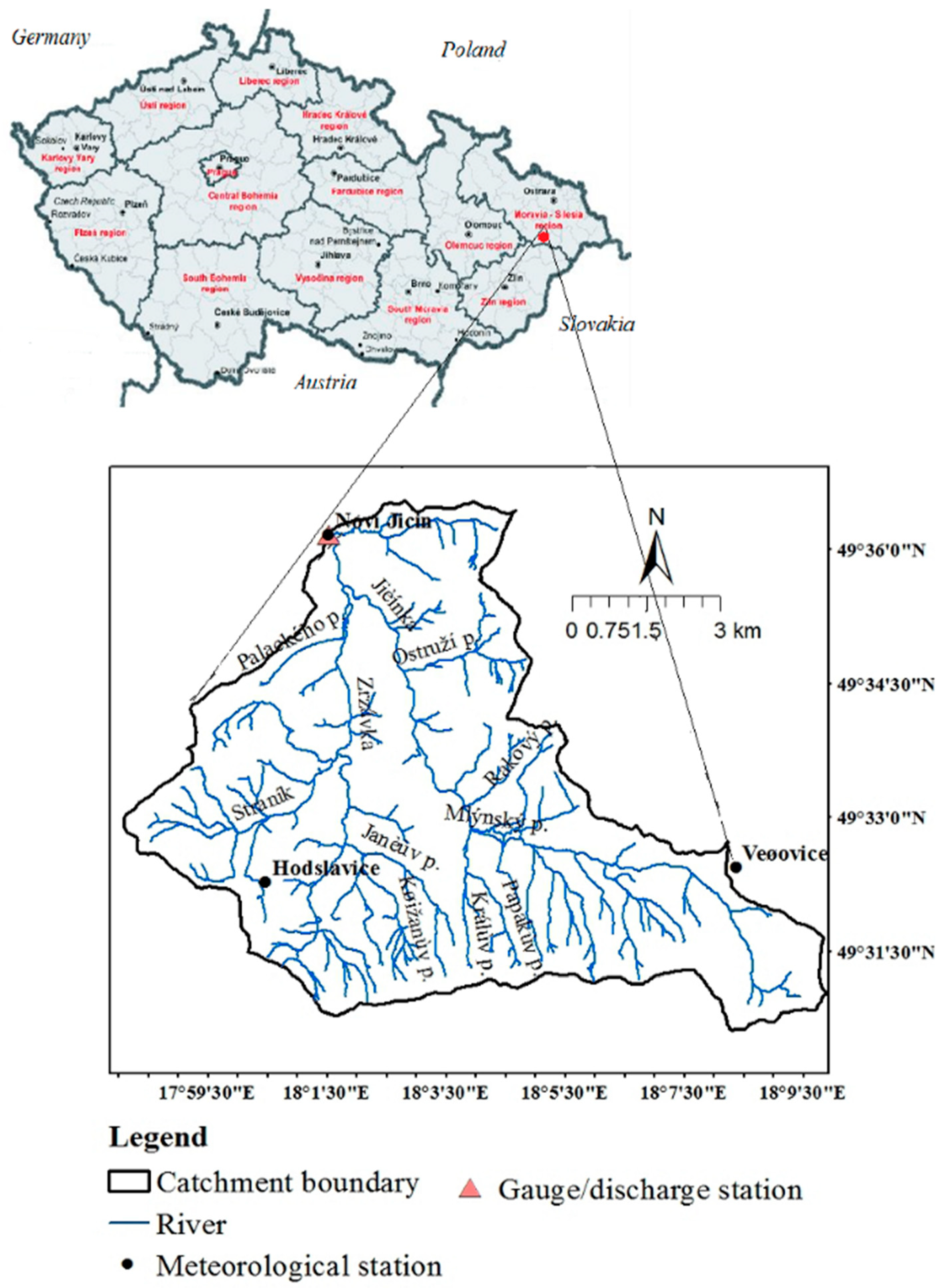
The torrential Jičinka River basin up to the “Novy Jičin” water level monitoring station (w.l.m.s) (Figure 1) is situated in the Moravian-Silesian Region, in the eastern part of the Czech Republic. It is also presented in Đukić et al. [31]. Altitudes in the Jičinka River basin vary from 270 m above sea level in the lower part of the basin to 1000 m in the source areas of the basin.
Four pedological types of soil were identified in the studied basin: fluvisol (10.5%), eutric cambisol (46.2%), dystric cambisol (41.3%) and rendzina (2%) (Figure 2). The hydrogeological behaviour of the whole catchment is defined by the dominant presence of the tertiary and quaternary rocks (sandstones, schists, loess, sand and gravel) which occupy about 75% of the basin (Figure 2). Four different vegetation types identified in the Jičinka River catchment are: forest (34%), natural grasslands (31%), arable land (8.5%) and orchards (0.03%) (Figure 2). Urban areas occupy about 9.4% of the catchment area.
2.1.2. Input Data
Several flash floods occurred in the territory of the Czech Republic during the last decade of June and at the beginning of July 2009, and in May and June 2010 [44]. These flash floods, together with the flash flood from September 2007, and the intensive rain events which caused them, were considered in this study and used as the basic input data for the calibration and validation of the models. The flood from 2009 was especially destructive as the peak flows significantly exceeded 100-year of recurrence time in many sites. The hourly values of runoff are measured at the hydrological station “Novy Jičin”. The characteristics of precipitation and runoff are presented in Table 1 [31].
All input data and the corresponding input parameters used in SHETRAN and in HEC HMS are summarized in Table 2.
The satellite soil moisture data used in this study were taken from the European Space Agency (ESA) Climate Change Initiative (CCI) Soil Moisture (SM) project (http://www.esasoilmoisture-cci.org, (accessed on 10 March 2020)) [45] and are also described in Đukić et. al. [31].
2.2. Methodology
The applied methodology can be divided into several tasks: (1) Creating different variants of rainfall–runoff models using the HEC-HMS and the SHETRAN software; (2) Calibration and validation of the HEC-HMS and the SHETRAN model for each variant on the basis of the measured streamflow hydrographs at the catchment outlet; (3) Simulations of surface soil moisture using the SHETRAN and HEC-HMS model for different configurations of the models; (4) Validation of the models by comparing the simulated soil moisture values and the downscaled satellite soil moisture data; (5) Result analysis and evaluation of the SHETRAN and HEC-HMS model performance in respect of runoff and soil moisture.
Both the SHETRAN and HEC-HMS models were calibrated for the storm event which happened in September 2007. They were validated for the storm events that happened in June 2009, May 2010 and June 2010 in respect of runoff, while the models’ validation in respect of soil moisture was performed for all analyzed rain events.
2.2.1. The SHETRAN Model
SHETRAN is a 3D coupled surface/subsurface physically based and spatially distributed (PBSD) river basin model. SHETRAN (version V4.4.5) water flow component was used in this study. The water flow component consists of 4 modules: evapotranspiration/interception, overland/channel; variably saturated subsurface and snowmelt [46]. The components of interception and evapotranspiration were neglected in this study, because their influence is negligible in rain event models. Both the overland and channel flows are described by the diffusive wave approximation of the full St. Venant equations [47]. The continuity equation is as follows:
The momentum conservation is as follows:
where: t is time, x is the measured distance along the channel (m), Q is discharge (m3s−1), A is hydraulic area (m2), q is tributary outflow (m3s−1), h is channel depth (m), C is Chezy coefficient (m0.5s−1), R is the hydraulic radius (m) and α is the correction factor (-). The soil water movement in the unsaturated zone is described using the Richards equation [48].
2.2.2. The HEC-HMS Model
HEC-HMS is a conceptual hydrological model, which has been used as a reliable platform for developing different variants of lumped and semi-distributed models in many countries. In the HEC-HMS model, the basin is conceptually represented as a network of subareas connected by channel links. HEC-HMS is composed of three main components: the basin model, the meteorological model, control specifications and time-series data. The physical datasets describing the basin properties are stored in the basin model. The meteorological model includes data on precipitation, evapotranspiration and snowmelt. The calculation methods for different components of the rainfall–runoff processes including loss (runoff volume), transformation to direct runoff and baseflow should be defined in separate modules within the basin model. A comprehensive description of all HEC-HMS components can be found in the user manual [49].
In this study, runoff volume is simulated by employing the Soil Conservation Service (SCS) curve number method using the following equation:
where: Pe is the accumulated precipitation excess at time t (mm), P is the accumulated rainfall depth at time t (mm), Ia is the initial abstraction (mm), d is the potential maximum retention (mm), CN—curve number (-) and λ is the initial abstraction ratio (λ = 0.2–2.28) [50]. The SCS method in HEC-HMS includes the following parameters: the initial abstraction, Curve Number and the share of impervious area in the basin (Impervious (%)).
The values of Curve Number (CN) are related to land cover, soil type, hydrologic soil group and antecedent moisture conditions [51]. This model parameter affects the peak of the hydrograph in a way that a larger CN number causes larger peak flows, and vice-versa. Initial abstraction (Ia) generally includes canopy interception, surface retention, and rainfall infiltration prior to runoff onset, and it is estimated as a fraction of maximum basin retention. The CN values for average antecedent conditions that are commonly given in the literature refer to λ values of 0.2 [52]. However, the values of λ may differ [50] and should be estimated from the rainfall–runoff observations, if available. Otherwise, the parameter Ia should be one of the calibration parameters, as is the case in this paper.
The Clark’s unit hydrograph method [53] was used in this study to describe the transformation of the excess rainfall into direct runoff at the basin outlet. This method includes the continuity Equation (6) and the storage–discharge relationship for a linear reservoir (7):
where: U (t) denotes inflow in the reservoir at time t, I (t) is the outflow from the reservoir, V(t) the reservoir storage at time t, and R is the constant of the linear reservoir, which is a free model parameter. The Clark’s unit hydrograph method in HEC-HMS includes two free parameters: the time of concentration, tc (h), and the storage coefficient, R (h) [54]. It depends on the topography, geology and land use within the basin.
The baseflow recession model was used to simulate base flows in this study. It assumes that the falling limb of a hydrograph can be represented by an exponentially decreasing curve [49]:
where: Q0 is initial baseflow rate (initial condition) (m3s−1), and k is the recession constant (-) (a free model parameter). The recession constant defines the decreasing of the baseflow and takes values between 0 and 1. During the recession period of a flood event, a ratio to peak (RP) is needed to be determined in order to obtain the threshold flow at which the baseflow is calculated as a fraction of peak flow. Q0, k and RP are required parameters for the baseflow recession model.
The soil moisture changes Δω were estimated by applying Equation (9) in the HEC HMS model. This equation is based on the Green–Ampt method [55] and on several assumptions. In order to determine the average change in soil moisture it was assumed that the layer of water on soil surface is equal to the excess precipitation.
where: i (t) is the infiltration intensity (mm/h), k is the filtration coefficient (mm/h), Hk is the capillary potential (mm), h0 is the surface water layer (mm), F (t) is the cumulative amount of infiltrated water since the beginning of the episode (mm).
2.2.3. Intercomparison of the SHETRAN and the HEC HMS Model Characteristics
The SHETRAN and the HEC HMS model were compared and evaluated in this study because of their different structural characteristics and different representation of the considered hydrological processes.
All hydrological models have two major components, the first one dealing with the conversion of rainfall into the runoff and base flow and the second one dealing with the routing of runoff and base flow to the catchment outlet as streamflow [56,57,58,59]. The Soil Conservation Service—Curve Number (CN) method used in the HEC HMS model is a simple and efficient method for estimating the approximate amount of runoff from a rainfall event in a particular area. It is also the method used in many other rainfall–runoff models. However, the main limitation of this method is the representation of the catchment characteristics (soil type, land use and antecedent moisture conditions) by the value of a single CN parameter. In addition, the adoption of three levels of soil moisture leads to rapid changes in the value of the CN parameter [60]. On the other hand, the use of the Richards equation for the estimation of infiltration in the unsaturated zone in the SHETRAN model enables detailed information about infiltration processes and a more accurate estimation of excess rainfall.
The Saint-Venant equations [47] are used for routing overland flow in both the HEC HMS and the SHETRAN model. However, the kinematic-wave approximation of the Saint-Venant equations was used in the HEC HMS model, while their diffusion-wave approximation was used in the SHETRAN model. The kinematic-wave approximation considers only the gravity and friction effects, while the diffusion-wave approximation contains the pressure term along with the frictional and gravity force terms. Therefore, the diffusion-wave approximation is a more reliable equation for routing overland flow as it takes the backwater effects and attenuation into consideration [61]. In spite of that, it was also stated in Ponce et al. [61] that in regions where backwater is not an important phenomenon, kinematic wave models give similar results to the diffusion-wave model because the numerical solution of the kinematic wave model is identical to the analytic solution of the diffusion-wave model.
2.2.4. The Catchment Subdivision
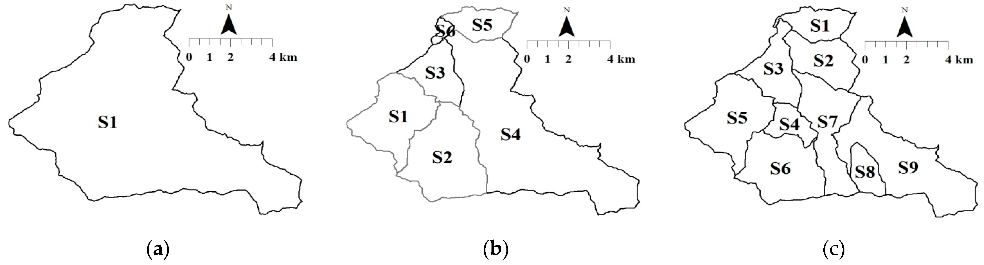
The variants of the HEC-HMS model include two models of different characters. The first variant is a lumped parameter model where the parameters are calculated as means across the catchment. The second and the third variant are the semi-distributed models containing 6 and 9 subcatchments, respectively (Figure 3). In the HEC-HMS model the discretization over the catchment area is conducted based on the pre-processing software GeoHMS, an add-on of ArcGIS.
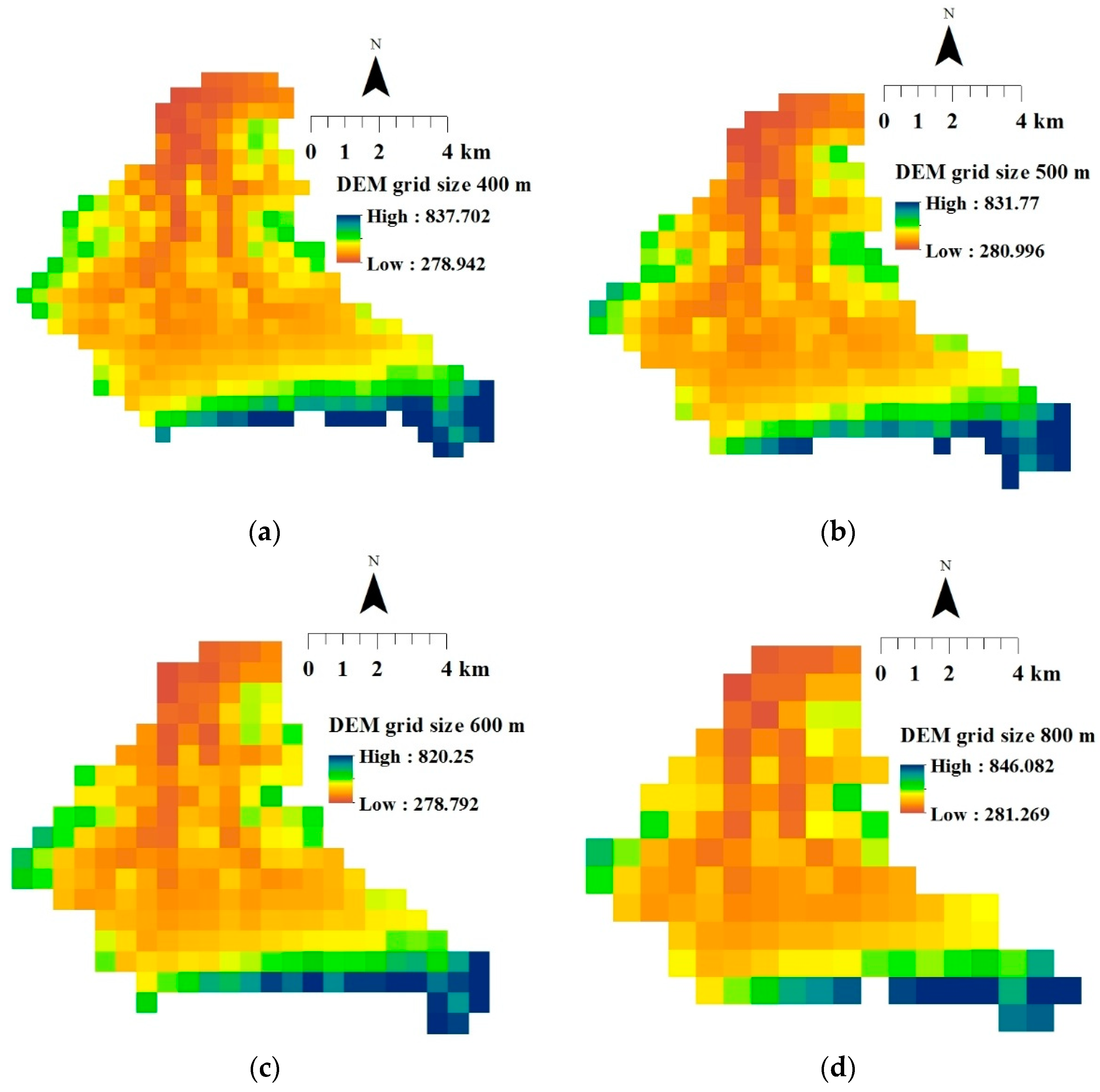
In case of the SHETRAN model, different variants of distributed models were created with four sets of digital maps with grid sizes of 400, 500, 600 and 800 m (Figure 4). The GIS software and its spatial analyst were used to extract the hydrological model parameters from DEM, soil and land use maps for the SHETRAN model.
2.2.5. Calibration of the SHETRAN Model
Taking into account that uncertainties in the evaluation of model parameters are very expressive in mountainous catchments [62,63], the sensitivity analysis of the SHETRAN model was performed for the purpose of reducing parameter dimensions. The adopted values of all parameters used in the SHETRAN model, for the grid cell size of 500 m, are presented in Table 3. In the case of the SHETRAN model, the same optimal values of model parameters used in calibration and validation were obtained at each grid resolution, except for the Strickler’s coefficients for overland flow and for river flow. For the grid cell sizes of 400, 500, 600 and 800 m, the obtained average values of the Strickler’s coefficients for overland flow are: 18, 25, 28 and 35, respectively and the Strickler’s coefficients for river flow are 25, 30, 38 and 45, respectively. In that way, the primary effect of increasing grid cell size is to require an increase in overland and channel Strickler’s roughness coefficient. It can be concluded that the coarser grid cell resolutions can be used for runoff simulations as long as parameters are appropriately calibrated.
2.2.6. Calibration of the HEC HMS Model
The values of the following parameters were estimated in the process of the HEC HMS model calibration and validation: Curve Number (CN), initial abstraction (Ia), time of concentration (tc), storage coefficient (R), recession constant (k) and ratio to peak (RP). The initial values of curve number (CN) were obtained for each sub-catchment using raster maps prepared from the previously created soil hydrologic group (HSG) layer and the land-use layer in the ArcGIS 10.2.2 software. For each type of soil, the hydrologic soil group was defined based on its known texture and the known percentage share of sand, silt and clay following the guidelines provided in the National Engineering Handbook of Hydrology [64]. The values of the CN number were assigned to each possible combination of land use and soil group obtained by overlapping the hydrologic soil group and the land use layer. The averaged values of the CN number were calculated for each sub-catchment area. Thus obtained values represented the initial values of the CN number used in the calibration process.
Initial estimates of the time of concentration tc and storage coefficient R were computed using the following empirical formula of Kirpich [65] and Clark [53], respectively:
where: L is the length of stream in km, S represents the land slope of basin (-) and α is the coefficient (value varies from 0.4 to 1.4). Both model parameters affect hydrograph shape and peak flow.
The initial and adopted values of calibrated model parameters are shown in Table 4. It should be noted that the values of initial abstraction depend on the variations in antecedent moisture conditions. The values of antecedent moisture conditions can be different for different rain evens. The obtained optimal values of initial abstraction that are shown in Table 4 refer to the calibration rain event in September 2007. The zero values of initial abstraction were adopted for the validation rain events in June 2009, May 2010 and June 2010. During the validation rain events, the soil was saturated and it was not able to receive an additional amount of water. The obtained optimal values of other model parameters were constant for both the calibration and validation rain events.
The effects of the catchment subdivisions on the HEC-HMS model calibrated parameters are primarily manifested on the parameters of the model of transformation of effective precipitation into a runoff. The reduction of the size of the sub-catchment’s area with the increasing number of the sub-catchments leads to the decrease of the length of the main flow, and the time of concentration and storage coefficient related to that, and vice versa. Although it was noticed that these parameters have the greatest impact on the volume and the peak of the hydrographs, the influence of these parameters was reduced for the higher number of sub-catchments. The loss model has quite similar values for all the catchment configurations. Besides that, the baseflow model’s parameters proved to be fixed parameters for the analyzed configurations of the catchment subdivision.
2.2.7. The Methodology Applied for the Comparison of Soil Moisture Estimates
Surface soil moisture simulations were performed using the sets of parameters optimized for the calibration and the validation rain events in respect of runoff. Surface soil moisture simulations were performed for four analyzed resolutions of grid cell size (400, 500, 600 and 800 m) by applying the SHETRAN model and for three different configurations of catchment subdivision by applying the HEC HMS model (lumped model, 6 sub-catchments and 9 sub-catchments).
The simulated values of soil moisture obtained by applying the SHETRAN model refer to the average values of soil moisture within each grid cell. On the other hand, the simulated HEC-HMS soil moisture values refer to the averaged soil moisture values at the levels of the discretized sub-catchments. In order to compare the simulated soil moisture values obtained by applying the two models, the SHETRAN soil moisture values were also averaged at the levels of discretized sub-catchments. The satellite retrieved soil moisture data were downscaled at the levels of the discretized sub-catchments by applying the method developed by Qu et al. [66]. This method as well as the procedure of downscaling were also described in Đukić et. al. [31].
2.2.8. Evaluation of Models Performances
The agreement between the modelled and observed runoff was evaluated using the following objective functions. The first objective function is based on the formulation proposed by Nash and Sutcliffe [67] and is given by:
where: Qobs, i is the observed streamflow on day i, Qsim, i is the simulated streamflow, is the average of the observed streamflow over the calibration (or verification) periods of n days.
Due to the changeable variance of model errors, the Nash–Sutcliffe coefficient of efficiency tends to emphasize the large errors. For comparison, the function of Chiew and McMahon [68] was used as the second objective function in which the square root of the considered values was related using the following equation:
The third introduced criterion [69] is potentially useful in the context of prediction, for example, where simulations must be as close as possible to the observed values at each time step. It is defined by:
The fourth criterion [70] quantifies the ability of the model to accurately reproduce streamflow volumes over the periods of observation. Criterion CR4 differs from the other three criteria (CR1–CR3), because it does not measure deviation from the observed values at each step of the simulation. Therefore, CR4 cannot be used alone as a criterion for calibration. This criterion is defined by:
In addition to the already mentioned four criteria (CR1–CR4) the following statistical measures were also used: the root-mean-square error (RMSE), the mean absolute error (MAE), the coefficient of correlation (R) and the index of agreement (d). They are expressed by the following equations:
The consistency between the soil moisture values simulated by the hydrologic models and the soil moisture values downscaled from the satellite retrieved soil moisture product was spatially analyzed using the criteria CR4, MAE, RMSE, R and d (Equations (15)–(19)). However, instead of comparing between the simulated (Qsim) and the observed streamflows (Qobs), in this case, the simulated and the downscaled satellite soil moisture data are compared. As it was explained in Đukić et al. [31], the criteria CR1, CR2 and CR3 were not used when comparing soil moisture estimates, not because the obtained negative values indicate the lack of agreement between the simulated and the satellite-derived soil moisture estimates, but because spatial and temporal differences in soil moisture are small in very wet conditions which prevail during the analyzed intensive rain events.
3. Results
3.1. Evaluation and Comparisons of Model Performances in Respect of the Simulations of Streamflow Hydrographs
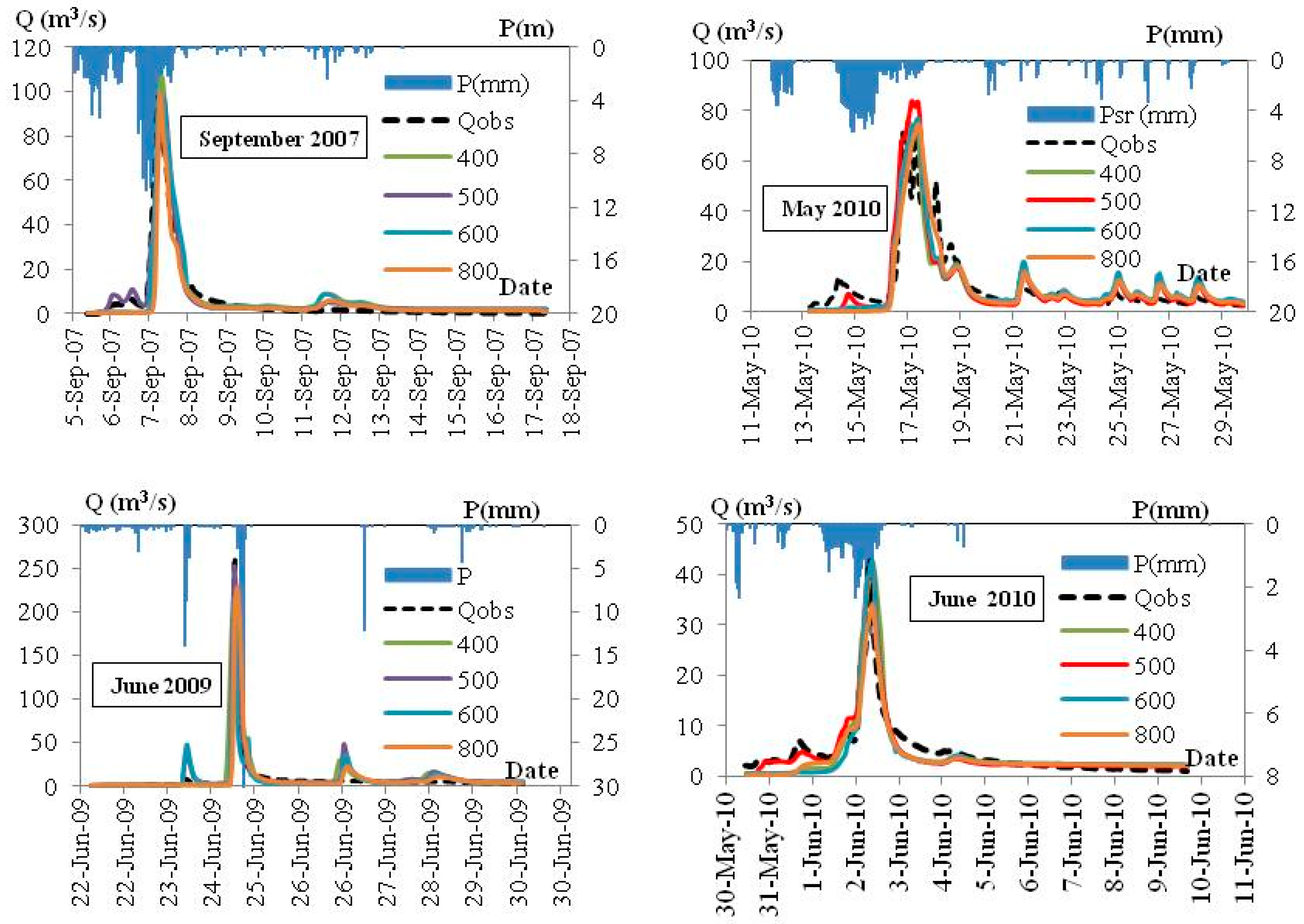
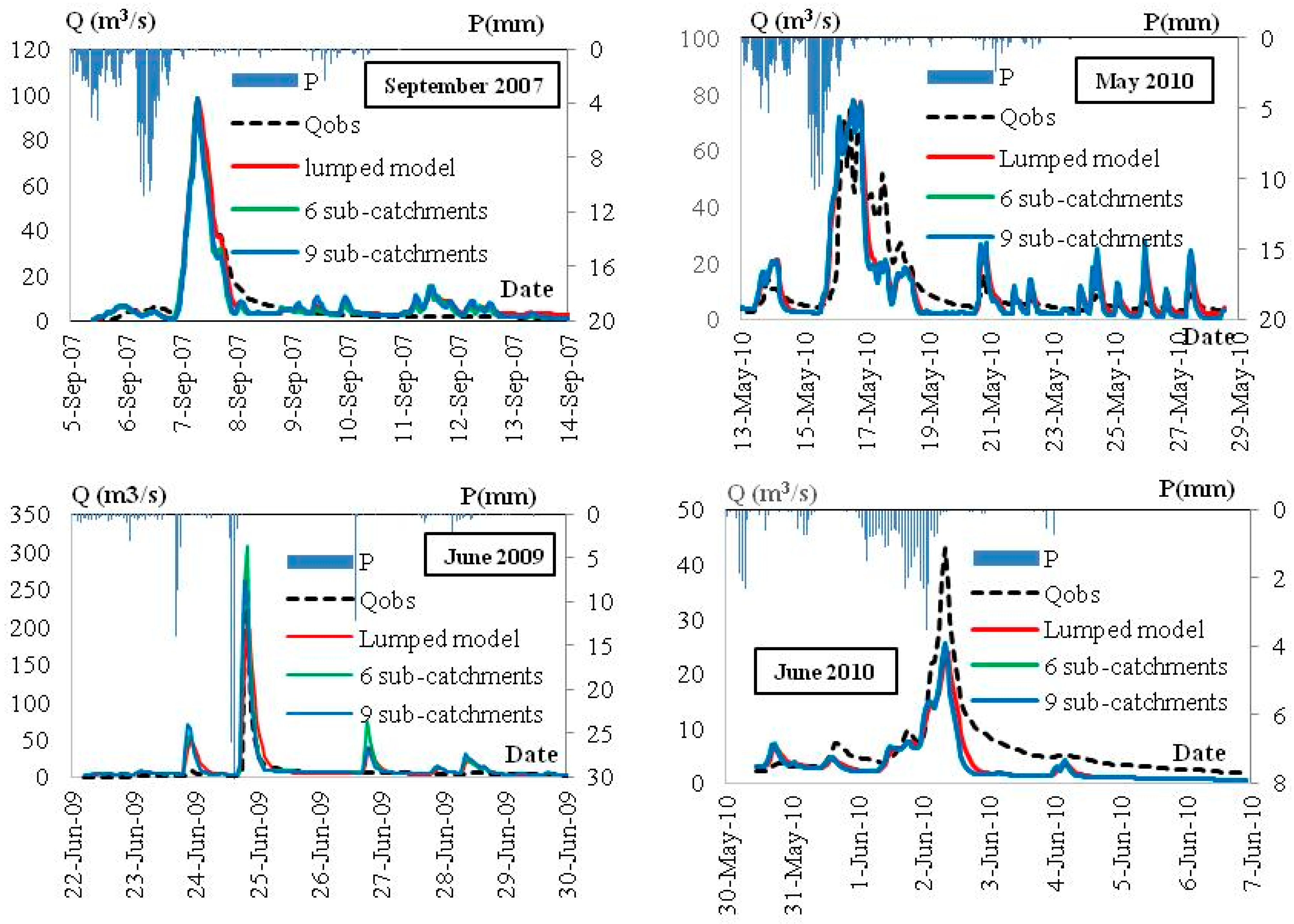
Figure 5 shows the results of the HEC HMS model calibration and validation for three different configurations of the catchment discretization, while the results of the SHETRAN model calibration and validation for four analyzed sizes of grid cells are presented in Figure 6. The results of quality assessment of the HEC HMS and SHETRAN model simulations in respect of streamflows according to the applied evaluation criteria are presented in Table 5 and Table 6, respectively.
When analyzing the effects of different configurations of the HEC HMS model on the HEC HMS model performance (Table 5), the lumped-based configuration showed a slightly better performance than the sub-catchment configurations with 6 and 9 sub-catchments. The observed model performances for the configurations with 6 and 9 sub-catchments are almost equal. Similarly, the effects of the HEC HMS model structures on the accuracy of flood simulations were also analyzed in the study Walega et al. [22]. It was also observed that more reliable flood simulation results were obtained in the lumped model configuration than in the semi-distributed configurations of this model.
When analyzing the effects of grid cell size on the SHETRAN model performance in respect of streamflow hydrographs (Table 6), the best performance measures were observed for the grid cell size of 500 m, followed by the performance measures for the grid cell size of 600 m, while the performance measures for the grid cell size of 800 m are lower for both the calibration and validation periods.
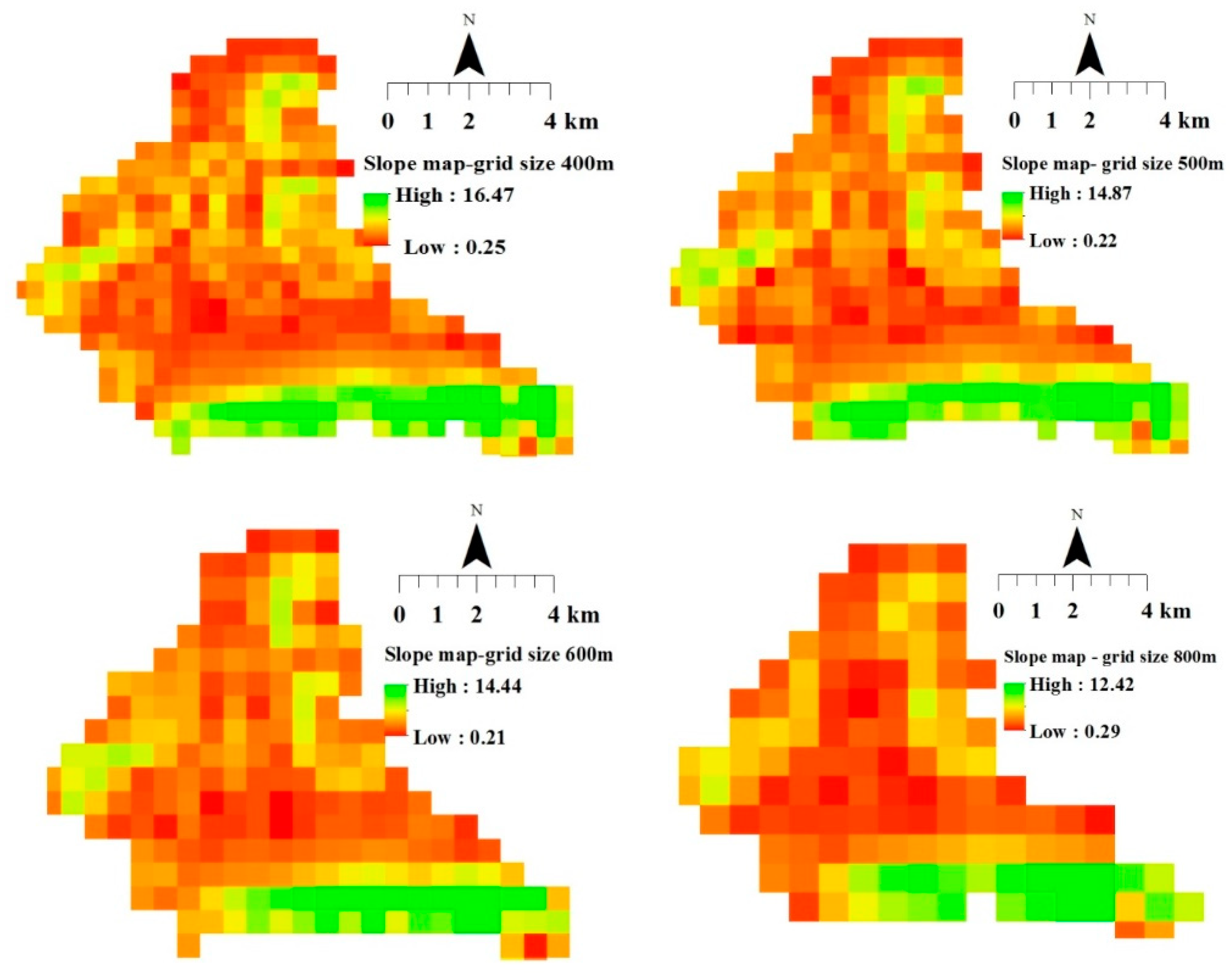
It can also be noticed that the obtained satisfactory results of the SHETRAN model calibration and validation at all analyzed resolutions of grid cell size indicate that the coarser grid cell resolutions can be used in rainfall–runoff simulations if parameters are properly calibrated. Besides that, the results, obtained after numerous simulations in this study, indicate that coarser grid sizes are more appropriate when simulating high-intensity rain events such as the rain events analyzed in the Jičinka River catchment. It can be seen that the primary effect of increasing grid cell size on simulation parameters is to require an increase in the overland and channel Strickler’s coefficients. The same conclusions were obtained in the study Molnar and Julien [30]. Molnar and Julien [30] analyzed the effects of grid cell size on surface runoff modelling using a distributed hydrologic CASC 2D model, on the examples of two small watersheds in northern Mississippi. The obtained results in that study also indicate that coarser grid sizes are more appropriate when simulating rain events of high intensity. The increase in the overland and channel Strickler’s coefficients with the increase of grid cell size is related to the representation of watershed characteristics influencing the overland and channel flow. This increase is a result of the combined influence of flow length, slope, hydraulic radius and stream roughness. The area covered by the stream network becomes larger with the increase of cell size resulting in the increase in the overland and channel Strickler’s coefficient. The increase in grid cell size resulted in a significant underestimation of slope values. It was observed that the mean slope decreases from 0.08 for a 400 m DEM, to 0.057 for an 800 m DEM (Figure 7). The area with slope values higher than 0.100 is 22.4% of the total catchment area for a 400 m DEM, while this percentage decreases to 18.8%, 13.7% and 12.1% respectively for a 500, 600 and 800 m resolution DEM.
On the basis of Figure 5 and Figure 6 and Table 5 and Table 6, it can be concluded that satisfactory agreement was found between the observed and simulated streamflow hydrographs obtained by applying both the SHETRAN and the HEC HMS model in cases of all the analyzed configurations of catchment discretization and for all the analyzed rain events. However, better performance measures were obtained the physically based and distributed SHETRAN model was applied than by applying the lumped and semi-distributed configurations of the HEC HMS model. It should also be noted that for both models, the best performance measures were observed for the calibration rain event in September 2007 according to the majority of applied criteria. It can also be seen that due to a small decrease in the determined values of the applied evaluation criteria from calibration to verification, model robustness is slightly decreased in the case of both models.
3.2. Evaluation and Comparisons of Model Performances in Respect of Soil Moisture Estimates
The results of the assessment of the quality of the HEC HMS and SHETRAN models simulations in respect of soil moisture according to the applied evaluation criteria are presented in Table 7 and Table 8.
When analysing the HEC HMS model performance for different model configurations in respect of soil moisture, the best performance measures were obtained for the model configuration consisting of six sub-catchments (Table 7). The obtained performance measures are slightly lower for the HEC HMS lumped model, and even lower for the configuration consisting of nine sub-catchments.
When analyzing the SHETRAN model performance for different grid cell sizes the best performance measures were obtained for the grid cell size of 500 m according to the majority of applied criteria for all the analyzed rain events (Table 8).
Based on Table 7 and Table 8 it can be seen that good agreement was observed between the simulated daily values of soil moisture values and the downscaled satellite values of soil moisture for all analyzed configurations of catchment discretization in the case of the HEC HMS model and for all four analyzed sizes of grid cells in the case of the SHETRAN model. The simulated values of soil moisture obtained for the lumped configurations of the HEC HMS and SHETRAN models also agree well with the downscaled satellite soil moisture values for the majority of applied criteria. However, the obtained values of the Correlation coefficient and the Index of agreement are lower in the case of the SHETRAN lumped configuration than in the case of the HEC HMS lumped configuration.
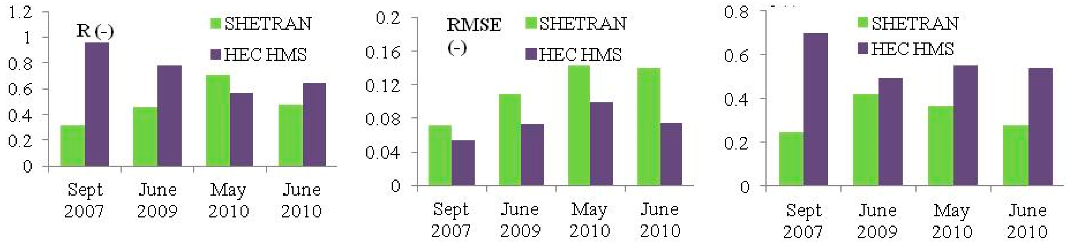
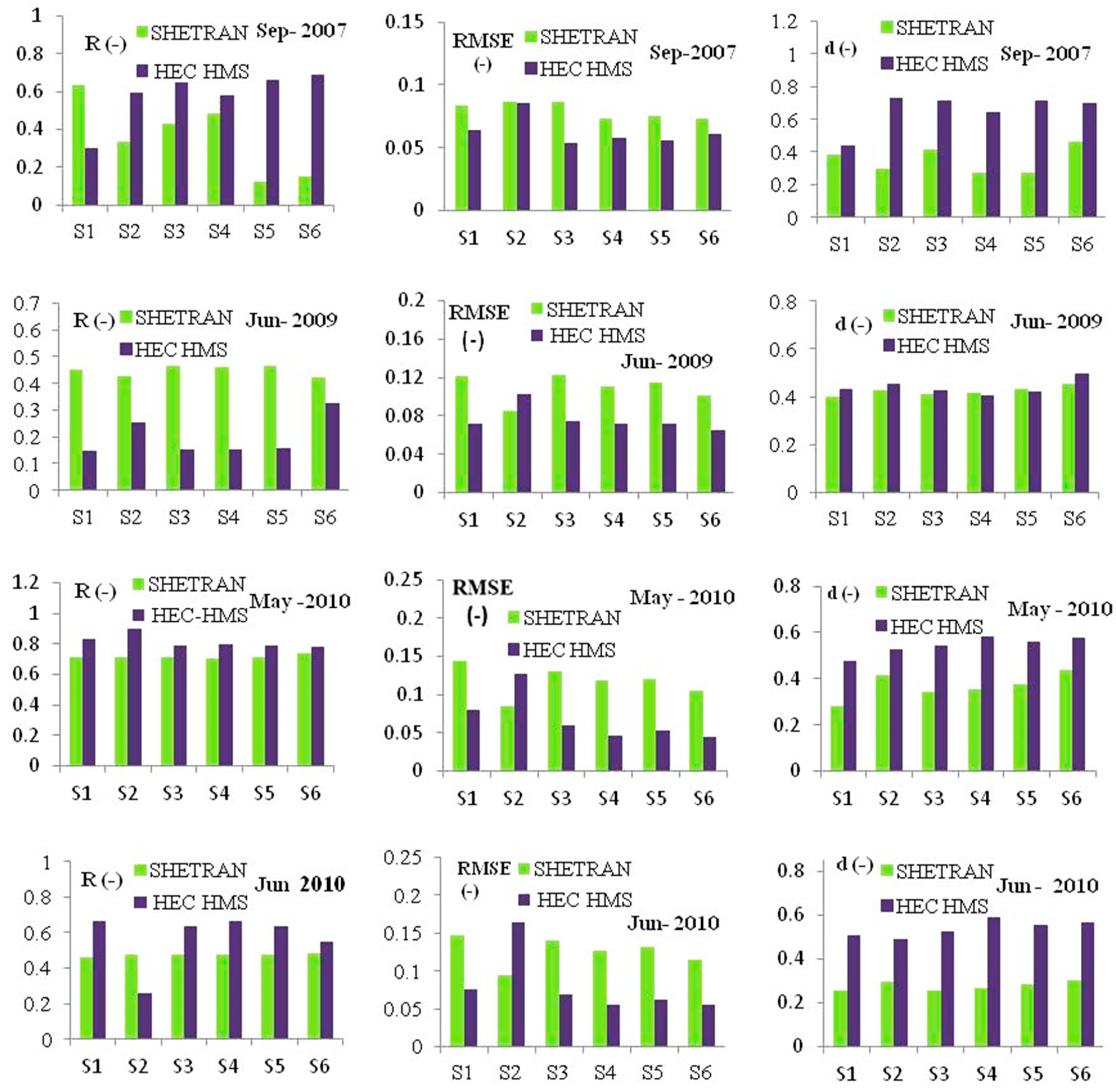
Comparative overview of the performance measures in respect of soil moisture obtained for the different configurations of the HEC HMS and SHETRAN model application for the Jičinka River catchment (the Correlation Coefficient, the Root Mean Square Error and the Index of agreement) for the analyzed rain events in September 2007, June 2009, May 2010 and in June 2010 are also presented in Figure 8, Figure 9 and Figure 10.
When comparing the SHETRAN and the HEC HMS model in respect of soil moisture it can be seen that better performance measures were achieved by application the semi-distributed HEC HMS model for the catchment discretization into six sub-catchments than by application the distributed SHETRAN model according to the majority of the applied evaluation criteria.
When analyzing the values of evaluation criteria for the lumped model configurations (Figure 8) and along the discretized sub-catchments (Figure 9 and Figure 10) it can also be concluded that better performance measures were obtained mostly by application of the HEC HMS model than by the application of the SHETRAN model. While in the case of the catchment discretization into six sub-catchments, the performance measures are consistent along the sub-catchments, in the case of the catchment discretization into nine sub-catchments, some inconsistencies were noticed along the sub-catchments denoted by S6 and S4. For these sub-catchments, the obtained values of the RMSE and d are better for the SHETRAN model than for the HEC HMS model. It should also be noted that the obtained performance measures for all analyzed model configurations are mostly better for the calibration period than for the validation periods.
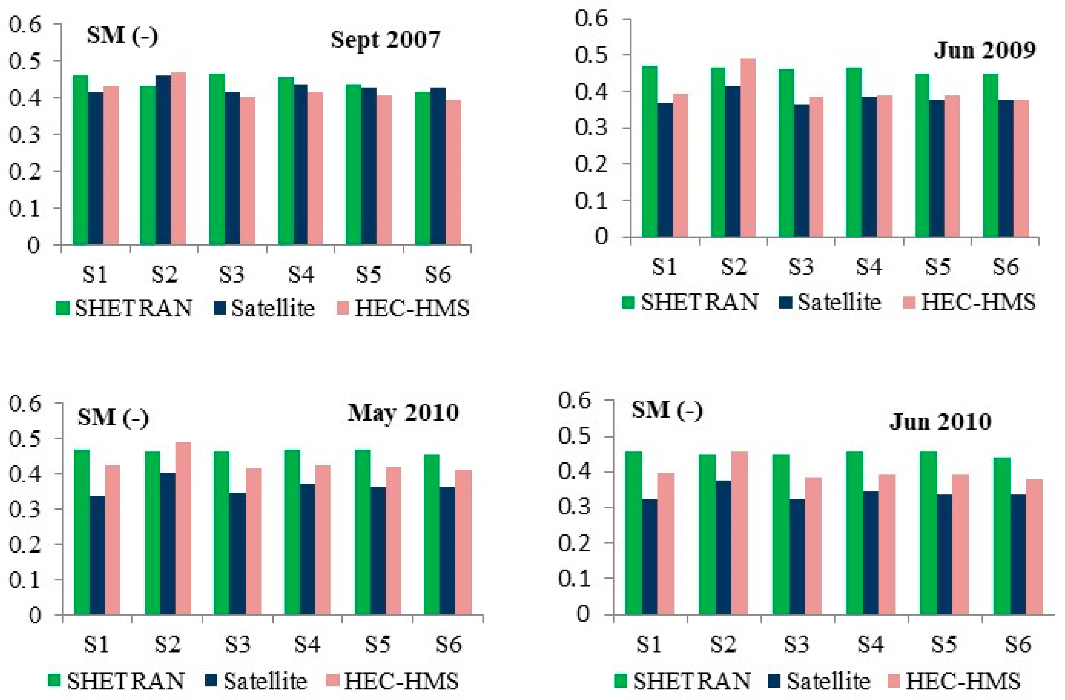
The comparative overview of the average soil moisture values, SM (-), within the sub-catchments of the Jičinka River catchment obtained by downscaling of satellite soil moisture data and for optimal configurations of the SHETRAN and the HEC HMS model for the analyzed rain events in September 2007, June 2009, May 2010 and June 2010 are presented in Figure 11.
The results obtained in this study indicate that the more complex SHETRAN model performed better in streamflow simulations, while the less complex HEC HMS model performed better in respect of soil moisture simulations. The obtained results are in agreement with the results obtained in Orth et al. [29] and in Li et al. [28]. In the study Li et al. [28] different variants of the HBV model were compared in terms of complexity according to runoff simulations at the catchment outlet and the interior points and according to the simulations of internal processes of evapotranspiration, snow water and groundwater depth of a mountainous catchment in Norway. In the study Orth et al. [29], three hydrological models of different complexity (HBV, PREVAH and SWBM) were validated and compared in terms of runoff and soil moisture at several locations across Switzerland. Similar to the results obtained in this study, the common conclusion of these studies is that models with higher complexity can improve runoff simulations. However, it was also observed that the performance of complex grid models is not higher over simpler models in reproducing internal variables [28].
It should be noted that in this study the variability of soil moisture over the Jičinka River catchment was estimated by applying two alternative methods of estimating soil moisture: hydrological models and satellite soil moisture observations. Although there is a substantial amount of uncertainty in soil moisture estimates from these two sources of soil moisture information, good agreement between the obtained soil moisture values was observed. Based on the above, it can be concluded that the joint application of a hydrological model of appropriate structure and remotely sensed soil moisture information contributes to improving rainfall–runoff modeling in small and ungauged catchments.
4. Conclusions
In this study, the two models of different complexity, the more complex SHETRAN and the simpler HEC HMS model, and their different configurations were compared and evaluated in respect of streamflow and soil moisture simulations on the example of the small torrential Jičinka River catchment in the Czech Republic (75.6 km2). The comparisons of streamflow simulations were performed on the basis of the registered streamflow hydrographs at the catchment outlet, while the soil moisture estimates were compared with the downscaled satellite surface soil moisture data as the reference data. The results have shown that although both SHETRAN and HEC HMS have produced reasonable results, SHETRAN performed better in streamflow simulations comparing to both the lumped and semi-distributed variants of the HEC HMS model. It was also observed that the semi-distributed configurations of the HEC HMS model outperform the SHETRAN model in soil moisture simulations, in spite of the use of more complex and more physically based equations in the SHETRAN model.
When analyzing the effects of different grid sizes of the SHETRAN model on the SHETRAN model results, the best results were obtained for the grid cell size of 500 m in both streamflow simulations and soil moisture simulations. When analyzing the effects of different HEC HMS model configurations on HEC HMS model results, the obtained performance measures for the lumped configuration are better in streamflow simulations, while the configuration with the six sub-catchment discretization resulted in better agreement with the downscaled surface soil moisture data.
Based on the analysis carried out in this study, it can be concluded that the additional complexity of hydrological models does not necessarily imply their improved performance and that performance can be changeable depending on the considered hydrological variable (e.g., runoff vs. soil moisture). The recommendations for further research refer to comparisons and evaluations of more calibration approaches, more model structures and more case studies. Future research should contribute to the development of new and more efficient models that would be useful for operational hydrology. Future models should be created by merging efficient components from different models into a single one with an appropriate structure.
The additional conclusion of this study is also that joint application of a hydrological model of appropriate structure and remotely sensed soil moisture information should help reduce the uncertainties in rainfall–runoff modeling and improve and facilitate the calibration and validation of hydrological models in spite of the uncertainties related to these two sources of soil moisture information. This study also shows that remotely sensed soil moisture data could be efficiently used for better evaluations of rainfall–runoff models in small and ungauged catchments. This modeling procedure was not previously applied to small catchments.
Author Contributions
Conceptualization, Data curation, Writing, V.Đ.; Formal analysis; Investigation, Methodology, Software, Validation, V.Đ. and R.E.; All authors have read and agreed to the published version of the manuscript.
Funding
This research was funded by the University of Belgrade, Faculty of Forestry.
Institutional Review Board Statement
Not applicable.
Informed Consent Statement
Not applicable.
Data Availability Statement
The data presented in this study are available on request from the corresponding author.
Acknowledgments
This paper was supported by the Ministry of Education, Science and Technological Development, Republic of Serbia.
Conflicts of Interest
The authors declare no conflict of interest.
References
- Pavlik, F.; Dumbrovský, M. Influence of landscape retention capacity upon flood processes in Jičínka River basin. Acta Univ. Agric. Silvic. Mendel. Brun. 2014, 62, 191–199. [Google Scholar] [CrossRef] [Green Version]
- Beven, K. A manifesto for the equifinality thesis. J. Hydrol. 2006, 320, 18–30. [Google Scholar] [CrossRef] [Green Version]
- Jakeman, A.J.; Hornberger, G.M. How much complexity is warranted in a rainfall-runoff model? Water Resour. Res. 1993, 29, 2637–2649. [Google Scholar] [CrossRef]
- Bergström, S.; Lindström, G.; Pettersson, A. Multi-variable parameter estimation to increase confidence in hydrological modelling. Hydrol. Process. 2002, 16, 413–421. [Google Scholar] [CrossRef]
- Kirchner, J.W. Catchments as simple dynamic systems: Catchment characterization, rainfall-runoff modeling, and doing hydrology back-ward. Water Resour. Res. 2009, 45, W02429. [Google Scholar] [CrossRef] [Green Version]
- Đukić, V. Modelling of base flow of the basin of Kolubara river in Serbia. J. Hydrol. 2006, 327, 1–12. [Google Scholar] [CrossRef]
- Modrick Hansen, T.; Georgakakos, K. Intercomparison of lumped versus distributed hydrologic model ensemble simulations on operational forecast scales. J. Hydrol. 2006, 329, 174–185. [Google Scholar] [CrossRef]
- De Vos, N.J.; Rientjes, T.H.M.; Gupta, H.V. Diagnostic evaluation of conceptual rainfall-runoff models using temporal clustering. Hydrol. Process. 2010, 24, 2840–2850. [Google Scholar] [CrossRef]
- Mendez, M.; Calvo-Valverde, L. Development of the HBV-TEC hydrological model. Procedia Eng. 2016, 154, 1116–1123. [Google Scholar] [CrossRef] [Green Version]
- Darbandsari, P.; Coulibaly, P. Inter-comparison of lumped hydrological models in data-scarce watersheds using different precipitation forcing data sets: Case study of Northern Ontario, Canada. J. Hydrol. Reg. Stud. 2020, 31, 100730. [Google Scholar] [CrossRef]
- Wijayarathne, D.B.; Coulibaly, P. Identification of hydrological models for operational flood forecasting in St. John’s, Newfoundland, Canada. J. Hydrol. Reg. Stud. 2020, 27, 100646. [Google Scholar] [CrossRef]
- Petroselli, A. A generalization of the EBA4SUB rainfall–runoff model considering surface and subsurface flow. Hydrol. Sci. J. 2020, 65, 2390–2401. [Google Scholar] [CrossRef]
- Srivastava, A.; Deb, P.; Kumari, N. Multi-Model Approach to Assess the Dynamics of Hydrologic Components in a Tropical Ecosystem. Water Resour. Manag. 2020, 1–15, 327–341. [Google Scholar] [CrossRef]
- Suliman, A.H.A.; Jajarmizadeh, M.; Harun, S.; Mat Darus, I.Z. Comparison of Semi-Distributed, GIS-Based Hydrological Models for the Prediction of Streamflow in a Large Catchment. Water Resour. Manag. 2015, 29, 3095–3110. [Google Scholar] [CrossRef]
- Tegegne, G.; Park, D.K.; Kim, Y.; Kim, Y.-O. Selecting hydrologic modelling approaches for water resource assessment in the Yongdam watershed. J. Hydrol. 2017, 56, 155. [Google Scholar]
- Tegegne, G.; Park, D.K.; Kim, Y.-O. Comparison of hydrological models for the assessment of water resources in a data-scarce region, the Upper Blue Nile River Basin. J. Hydrol. Reg. Stud. 2017, 14, 49–66. [Google Scholar] [CrossRef]
- Vansteenkiste, T.; Tavakoli, M.; Van Steenbergen, N.; De Smedt, F.; Batelaan, O.; Pereira, F.; Willems, P. Intercomparison of five lumped and distributed models for catchment runoff and extreme flow simulation. J. Hydrol. 2014, 511, 335–349. [Google Scholar] [CrossRef]
- Zhang, L.; Xin, J.; He, C.; Zhang, B.; Zhang, X.; Li, J.; Zhao, C.; Tian, J.; DeMarchi, C. Comparison of SWAT and DLBRM for Hydrological Modeling of a Mountainous Watershed in Arid Northwest China. J. Hydrol. Eng. 2016, 21, 04016007. [Google Scholar] [CrossRef]
- Perrin, C.; Michel, C.; Andreassian, V. Does a large number of parameters enhance model performance? Comparative assessment of common catchment model structures on 429 catchments. J. Hydrol. 2001, 242, 275–301. [Google Scholar] [CrossRef]
- Grimaldi, S.; Nardi, F.; Piscopia, R.; Petroselli, A.; Apollonio, C. Continuous hydrologic modelling for design simulation in small and ungauged basins: A step forward and some tests for its practical use. J. Hydrol. 2020. [Google Scholar] [CrossRef]
- Zhang, H.; Wang, Y.J.; Wang, Y.Q.; Li, D.; Wang, X. The effect of watershed scale on HEC-HMS calibrated parameters: A case study in the Clear Creek watershed in Iowa, US. Hydrol. Earth Syst. Sci. Discuss. 2013, 10, 965–998. [Google Scholar] [CrossRef] [Green Version]
- Walega, A.; Leszek, K. The effect of a hydrological model structure and rainfall data on the accuracy of flood description in an upland catchment. Ann. Wars. Univ. Life Sci. Land Reclam. 2015, 47, 305–321. [Google Scholar] [CrossRef] [Green Version]
- Tripathi, M.P.; Raghuwanshi, N.S.; Rao, G.P. Effect of watershed subdivision on simulation of water balance components. Hydrol. Process 2006, 20, 1137–1156. [Google Scholar] [CrossRef]
- Muleta, M.K.; Nicklow, J.W.; Bekele, E.G. Sensitivity of a distributed watershed simulation model to spatial scale. J. Hydrol. Eng. 2007, 12, 163–172. [Google Scholar] [CrossRef]
- Kumar, S.; Merwade, V. Impact of watershed subdivision and soil data resolution on model calibration and parameter uncertainty. J. Am. Water Resour. Assoc. 2009, 45, 1179–1195. [Google Scholar] [CrossRef]
- Chen, F.; Xie, J.; Chen, X. Effects of spatial scale on distributed flood simulation based on HEC-HMS Model: A Case of Jinjiang Watershed, Fujian, China. In Proceedings of the 19th International Conference on Geoinformatics, Shanghai, China, 24–26 June 2011; pp. 1–5. [Google Scholar]
- Cleveland, T.G.; Luong, T.; Thompson, D.B. Watershed subdivision for modeling. In Proceedings of the World Environmental and Water Resources Congress, Great Rivers, Kansas City, MO, USA, 17–21 May 2009; pp. 6527–6536. [Google Scholar]
- Li, H.; Xu, C.; Beldring, S. How much can we gain with increasing model complexity with the same model concepts? J. Hydrol. 2015, 389, 858–871. [Google Scholar] [CrossRef] [Green Version]
- Orth, R.; Staudinger, M.; Seneviratne, S.I.; Seibert, J.; Zappa, M. Does model performance improve with complexity? A case study with three hydrological models. J. Hydrol. 2015, 523, 147–159. [Google Scholar] [CrossRef] [Green Version]
- Molnár, D.; Julien, P. Grid-Size Effects on Surface Runoff Modeling. J. Hydrol. Eng. 2000, 5, 8–16. [Google Scholar] [CrossRef]
- Đukić, V.; Erić, R.; Dumbrovsky, M.; Sobotkova, V. Spatio-temporal analysis of remotely sensed and hydrological model soil moisture in the small Jičinka River catchment in Czech Republic. J. Hydrol. Hydromech. 2021, 69, 1–12. [Google Scholar] [CrossRef]
- Gallart, F.; Latron, J.; Llorens, P.; Beven, K. Using internal catchment information to reduce the uncertainty of discharge and baseflow predictions. Adv. Water Resour. 2007, 30, 808–823. [Google Scholar] [CrossRef]
- Fenicia, F.; McDonnell, J.J.; Savenije, H.H.G. Learning from model improvement: On the contribution of complementary data to process understanding. Water Resour. Res. 2008, 44. [Google Scholar] [CrossRef] [Green Version]
- Beven, K. On doing better hydrological science. Hydrol. Process. 2008, 22, 3549–3553. [Google Scholar] [CrossRef]
- Parajka, J.; Naeimi, V.; Bioschl, G.; Wagner, W.; Merz, R.; Scipal, K. Assimilating scatterometer soil moisture data into conceptual hydrologic models at the regional scale. Hydrol. Earth Syst. Sci. 2006, 10, 353–368. [Google Scholar] [CrossRef] [Green Version]
- Xiong, L.; Yang, H.; Zeng, L.; Xu, C. Evaluating Consistency between the Remotely Sensed Soil Moisture and the Hydrological Model-Simulated Soil Moisture in the Qujiang Catchment of China. Water 2018, 10, 291. [Google Scholar] [CrossRef] [Green Version]
- Srivastava, A.; Kumari, N.; Maza, M. Hydrological Response to Agricultural Land Use Heterogeneity Using Variable Infiltration Capacity Model. Water Resour. Manag. 2020, 34, 1–16. [Google Scholar] [CrossRef]
- Brocca, L.; Hasenauer, S.; Lacava, T.; Melone, F.; Moramarco, T.; Wagner, W.; Dorigo, W.; Matgen, P.; Martinez-Fernandez, J.; Llorens, P.; et al. Soil moisture estimation through ascat and amsr-e sensors: An intercomparison and validation study across europe. Remote Sens. Environ. 2011, 115, 3390–3408. [Google Scholar] [CrossRef]
- Wanders, N.; Bierkens, M.F.P.; De Jong, S.; Roo, A.; Karssenberg, D. The benefits of using remotely sensed soil moisture in parameter identification of large-scale hydrological models. Water Resour. Res. 2014, 50, 10215. [Google Scholar] [CrossRef] [Green Version]
- López López, P.; Sutanudjaja, E.H.; Schellekens, J.; Sterk, G.; Bierkens, M.F.P. Calibration of a large-scale hydrological model using satellite-based soil moisture and evapotranspiration products. Hydrol. Earth Syst. Sci. 2017, 21, 3125–3144. [Google Scholar] [CrossRef] [Green Version]
- Peng, J.; Loew, A.; Zhang, S.; Wang, J.; Niesel, J. Spatial downscaling of satellite soil moisture data using a Vegetation Temperature Condition Index. IEEE Trans. Geosci. Remote Sens. 2017, 54, 558–566. [Google Scholar] [CrossRef]
- Verhoest, N.E.C.; van den Berg, M.J.; Martens, B.; Lievens, H.; Wood, E.F.; Pan, M.; Kerr, Y.H.; Al Bitar, A.; Tomer, S.K.; Drusch, M.; et al. Copula-based downscaling of coarse-scale soil moisture observations with implicit bias correction. IEEE Trans. Geosci. Remote Sens. 2015, 53, 3507–3521. [Google Scholar] [CrossRef]
- Lievens, H.; Tomer, S.K.; Al Bitar, A.; De Lannoy, G.; Drusch, M.; Dumedah, G.; Franssen, H.J.; Kerr, Y.; Martens, B.; Pan, M. SMOS soil moisture assimilation for improved hydrologic simulation in the Murray Darling Basin, Australia. Remote Sens. Environ. 2015, 168, 146–162. [Google Scholar] [CrossRef]
- Danhelka, J.; Kubat, J.; Šercl, P.; Čekal, R. (Eds.) Floods in the Czech Republic in June 2013; Czech Hydrometeorological Institute: Prague, Czech Republic, 2014. [Google Scholar]
- Dorigo, W.A.; Wagner, W.; Albergel, C.; Albrecht, F.; Balsamo, G.; Brocca, L.; Chung, D.; Ertl, M.; Forkel, M.; Gruber, A.; et al. ESA CCI Soil Moisture for improved Earth system understanding: State-of-the art and future directions. Remote Sens. Environ. 2017, 203, 185–215. [Google Scholar] [CrossRef]
- Ewen, J.; Parkin, G.; O’Connell, P.E. SHETRAN: Distributed River Basin Flow and Transport Modelling System. ASCE J. Hydrol. Eng. 2000, 5, 250–258. [Google Scholar] [CrossRef] [Green Version]
- Saint-Venant, A. Théorie du mouvement non permanent des eaux, avec application aux crues des rivières et a l’introduction de marées dans leurs lits. C. R. Hebd. Séances Acad. Sci. 1871, 73, 147–154. [Google Scholar]
- Richards, L.A. Capillary Conduction of Liquids through Porous Mediums. J. Appl. Phys. 1931, 1, 318–333. [Google Scholar] [CrossRef]
- USACE. HEC Hydrologic Modelling System (HEC-HMS) v4.3 User’s Manual; US Army Corps of Engineers: Washington, DC, USA; Hydrologic Engineering Center: Davis, CA, USA, 2018. Available online: https://www.hec.usace.army.mil/software/hec-hms/documentation/HEC-HMS_Users_Manual_4.3.pdf (accessed on 20 June 2020).
- Petroselli, A.S.; Grimaldi, S.; Romano, N. Curve-Number/Green—Ampt mixed procedure for net rainfall estimation: A case study of the Mignone watershed, IT. Procedia Environ. Sci. 2013, 19, 113–121. [Google Scholar] [CrossRef] [Green Version]
- Chow, V.T.; Maidment, D.R.; Mays, L.W. Applied Hydrology; McGraw-Hill, Inc.: New York, NY, USA, 1988; Available online: http://ponce.sdsu.edu/Applied_Hydrology_Chow_1988.pdf (accessed on 20 January 2021).
- Woodward, D.E.; Hawkins, R.H.; Hjelmfelt, A.T.J.; Quan, Q.D. Runoff Curve Number Method: Examination of the Initial Abstraction Ratio. In Proceedings of the World Water & Environmental Resources Congress 2003, Philadelphia, PA, USA, 23–26 June 2003; ASCE: Philadelphia, PA, USA, 2003; pp. 1–10. Available online: http://ponce.sdsu.edu/hawkins_initial_abstraction.pdf (accessed on 20 January 2021).
- Clark, C.O. Storage and the unit hydrograph. Trans. ASCE 1945, 110, 1419–1488. [Google Scholar]
- Haan, C.T.; Barfield, B.J.; Hayes, J.C. Design Hydrology and Sedimentology for Small Catchments; Academic Press: Cambridge, MA, USA, 1994. [Google Scholar]
- Green, W.H.; Ampt, G.A. Studies in soil physics. Part 1. The flow of air and water through soils. J. Agric. Sci. 1911, 4, 1–24. [Google Scholar]
- Todini, E. Rainfall-runoff modeling—past, present and future. J. Hydrol. 1988, 100, 341–352. [Google Scholar] [CrossRef]
- Todini, E. Hydrological catchment modelling: Past, present, and future. Hydrol. Earth Syst. Sci. 2007, 11, 468–482. [Google Scholar] [CrossRef] [Green Version]
- Peel, M.C.; Bloschl, G. Hydrological modelling in a changing world. Prog. Phys. Geogr. 2011, 35, 249e261. [Google Scholar] [CrossRef]
- Paul, P.; Kumari, N.; Panigrahy, N.; Mishra, A.; Singh, R. Implementation of cell-to-cell routing scheme in a large scale conceptual hydrological model. Environ. Model. Softw. 2018, 101, 23–33. [Google Scholar] [CrossRef]
- Młyński, D.; Walega, A.; Ciupak, M.; Petroselli, A. New approach for determining the quantiles of maximum annual flows in ungauged catchments using the EBA4SUB model. J. Hydrol. 2020, 589, 125198. [Google Scholar] [CrossRef]
- Ponce, V.M.; Li, R.M.; Simons, D.B. Applicability of kinematic and diffusion models. J. Hydraul. Div. 1978, 104, 353–360. [Google Scholar] [CrossRef]
- Đukić, V.; Radić, Z. GIS Based Estimation of Sediment Discharge and Areas of Soil Erosion and Deposition for the Torrential Lukovska River Catchment in Serbia. Water Resour. Manage. 2014, 28, 4567–4581. [Google Scholar] [CrossRef]
- Đukić, V.; Radić, Z. Sensitivity Analysis of a Physically Based Distributed Model. Water Resour. Manag. 2016, 3, 1669–1684. [Google Scholar] [CrossRef]
- USDA; NRSC. National Engineering Handbook of Hydrology; United States Department of Agriculture: Washington, DC, USA; Natural Resources Conservation Service: Washington, DC, USA, 2007. Available online: https://www.nrcs.usda.gov/wps/portal/nrcs/detailfull/national/water/manage/hydrology/?cid=stelprdb1043063 (accessed on 15 January 2021).
- Kirpich, Z.P. Time of concentration of small agricultural watersheds. Civil Eng. 1940, 6, 362. [Google Scholar]
- Qu, W.; Bogena, H.R.; Huisman, J.A.; Vanderborght, J.; Schuh, M.; Priesack, E.; Vereecken, H. Predicting subgrid variability of soil water content from basic soil information. Geophys. Res. Lett. 2015, 42, 789–796. [Google Scholar] [CrossRef] [Green Version]
- Nash, J.E.; Sutcliffe, J.V. River flow forecasting through conceptual models: Part I. A discussion of principles. J. Hydrol. 1970, 27, 282–290. [Google Scholar] [CrossRef]
- Chiew, F.; McMahon, T. Application of the daily rainfall–runoff model MODHYDROLOG to 28 Australian catchments. J. Hydrol. 1994, 153, 383–416. [Google Scholar] [CrossRef]
- Ye, W.; Bates, B.C.; Viney, N.R.; Silvapan, M.; Jakeman, A.J. Performance of conceptual rainfall–runoff models in low-yielding ephemeral catchments. Water Resour. Res. 1997, 33, 153–166. [Google Scholar] [CrossRef]
- Pereira, A.R.; Pruitt, W.O. Adaptation of the Thornthwaite scheme for estimating daily reference evapotranspiration. Agric. Water Manag. 2004, 66, 251–257. [Google Scholar] [CrossRef]
Figure 1.
The Jičinka River catchment with the river system and the rain gauging and hydrological stations in the catchment.
Figure 1.
The Jičinka River catchment with the river system and the rain gauging and hydrological stations in the catchment.

Figure 2.
The map of soil types (a), the map of geological types (b), the map of vegetation types (c) and the slope map (d) of the Jičinka River basin up to the “Novy Jičin” w.l.m.s.
Figure 2.
The map of soil types (a), the map of geological types (b), the map of vegetation types (c) and the slope map (d) of the Jičinka River basin up to the “Novy Jičin” w.l.m.s.

Figure 3.
The analyzed configurations of the Hydrologic Modeling System (HEC-HMS) model: the lumped model (a) and the semi-distributed models with discretization into six sub-catchments (b) and nine sub-catchments (c).
Figure 3.
The analyzed configurations of the Hydrologic Modeling System (HEC-HMS) model: the lumped model (a) and the semi-distributed models with discretization into six sub-catchments (b) and nine sub-catchments (c).

Figure 4.
Spatial discretizations of the digital elevation model (DEM) of the Jičinka River catchment in the the Système Hydrologique Européen TRANsport (SHETRAN) model—grid sizes 400 (a), 500 (b), 600 (c) and 800 m (d).
Figure 4.
Spatial discretizations of the digital elevation model (DEM) of the Jičinka River catchment in the the Système Hydrologique Européen TRANsport (SHETRAN) model—grid sizes 400 (a), 500 (b), 600 (c) and 800 m (d).

Figure 5.
Observed (Qobs) and the HEC HMS model-simulated streamflow hydrographs for different configurations of catchment discretization (lumped model, six sub-catchments and nine sub-catchments) at the Jičinka River monitoring station (“Novy Jičin” w.l.m.s) for the calibration (September 2007) and validation (June 2009, May 2010 and June 2010) rain events.

Figure 6.
Observed (Qobs) and the SHETRAN model simulated streamflow hydrographs for the grid cell sizes 400, 500, 600 and 800 m at the Jičinka River monitoring station (“Novy Jičin” w.l.m.s) for the calibration (September 2007) and validation (June 2009, May 2010 and June 2010) rain events.
Figure 6.
Observed (Qobs) and the SHETRAN model simulated streamflow hydrographs for the grid cell sizes 400, 500, 600 and 800 m at the Jičinka River monitoring station (“Novy Jičin” w.l.m.s) for the calibration (September 2007) and validation (June 2009, May 2010 and June 2010) rain events.

Figure 7.
Slope maps obtained on the basis of DEMs of different grid cell sizes.

Figure 8.
Comparative overview of the performance measures obtained by the SHETRAN and HEC HMS lumped models application in respect of soil moisture for the Jičinka River catchment (the Correlation Coefficient, the Root Mean Square Error and the Index of agreement for the analyzed rain events in September 2007, June 2009, May 2010 and in June 2010.

Figure 9.
Comparative overview of the performance measures for the sub-catchments of the Jičinka River catchment in respect of soil moisture obtained by applying the SHETRAN and HEC HMS models discretization with six sub-catchments (the Correlation Coefficient, the Root Mean Square Error and the Index of agreement) for the analyzed rain events in September 2007, June 2009, May 2010 and June 2010.

Figure 10.
Comparative overview of the performance measures for the sub-catchments of the Jičinka River catchment in respect of soil moisture obtained by applying the SHETRAN and HEC HMS models discretization with nine sub-catchments (the Correlation Coefficient, the Root Mean Square Error and the Index of agreement) for the analyzed rain events in September 2007, June 2009, May 2010 and June 2010.

Figure 11.
Comparative overview of the average soil moisture values within the sub-catchments of the Jičinka River catchment obtained by satellite soil moisture downscaling and by applying the SHETRAN and HEC HMS models (configuration with discretization in six sub-catchments) for the analyzed rain events in September 2007, June 2009, May 2010 and June 2010.


Table 1.
Total amounts of precipitation (Ptot) at the Jičinka River catchment fallen on the ground, the volume of precipitation (Vp), the maximum runoff value (Qmax) and the runoff volume (Vr).
Table 1.
Total amounts of precipitation (Ptot) at the Jičinka River catchment fallen on the ground, the volume of precipitation (Vp), the maximum runoff value (Qmax) and the runoff volume (Vr).
| The Number of Rain Event | The Simulation Period | Ptot (mm) | Vp (103 m3) | Qmax (m3/s) | Vr (103 m3) |
|---|---|---|---|---|---|
| 1 | 5 September 2007 (10:00)–7 September 2007(10:00) | 190.13 | 14429.9 | 98 | 6387.5 |
| 2 | 22 June 2009 (05:00)–29 June 2009 (7:00) | 150.2 | 11403 | 264 | 5805.5 |
| 3 | 11 May 2010(13:00)–29 May 2010 (3:00) | 232.8 | 17670.4 | 75.6 | 15666.4 |
| 4 | 30 May 2010 (11:00)–2 June 2010 (14:00) | 46.2 | 3502.2 | 43.1 | 4429.9 |
Table 2.
Input data and parameters used in the models.
| Type of Input Data | Input Parameters | Source of Input Data | |
|---|---|---|---|
| Meteorological | Hourly precipitation | Czech Hydrometeorological Institute | |
| Hydrological | Registered streamflow hydrographs | ||
| Topographic | Digital elevation model (DEM) of the resolution: 10 m × 10 m | T.G. Masaryk Water Research Institute | |
| SHETRAN: | HEC HMS | ||
| Land use/vegetation distribution | Strickler’s coefficient for overland flow (St) and for channel flow (StR) | Hydrologic soil group CN values Imperviousness | Corine Land Cover Databases https://land.copernicus.eu/pan-european/corine-land-cover (accessed on 20 June 2019) |
| Soil types | Hydraulic soil/rock properties (porosity and specific storage, residual water content (θr), saturated water content (θs), conductivity in unsaturated soil (kvs) saturated conductivity in saturated soil (khs) vanGenuchten-α, vanGenuchten-n | https://www.spucr.cz/bpej/celostatni-databaze-bpej (accessed on 20 June 2019) | |
| Geological type | “Czech Geological Survey”—ArcGIS online | ||
Table 3.
The ranges of model parameters used in the calibration of the SHETRAN model, its optimal values (in parenthesis) and the adopted values of uncalibrated parameters for the Jičinka River basin [31].
Table 3.
The ranges of model parameters used in the calibration of the SHETRAN model, its optimal values (in parenthesis) and the adopted values of uncalibrated parameters for the Jičinka River basin [31].
| Depth (m) | Texture | kvs (mday−1) | khs (mday−1) | Θs (-) | Θr (-) | α (-) | N (-) | St (m1/3s−1) | StR(m1/3s−1) | ||
|---|---|---|---|---|---|---|---|---|---|---|---|
| Dystric Cambisol | 0–0.7 | Sandy clay loam | 0.223–0.5814 (0.300) | 0.223–0.5814 (0.300) | 0.419–0.695 (0.480) | 0.047 | 0.014 | 1.317 | Forest | 4–8 (7) | 15–40 (30) |
| 8–20 (18) | |||||||||||
| 0.7–1.2 | Sandy clay loam | 0.223–0.5814 (0.300) | 0.223–0.5814 (0.300) | 0.419–0.695 (0.480) | 0.047 | 0.014 | 1.317 | Arable land | 7–18 (16) | ||
| Geol. substrate | 1.2–4 | schists | 4 | 0.01–5 (4) | 0.6 | 0.1 | 0.001 | 1.1 | Natural grasslands | 30–50 (42) | |
| Rendzina | 0–0.5 | Clay loam | 0.217–0.4105 (0.270) | 0.217–0.4105 (0.270) | 0.437–0.442 (0.440) | 0.075 | 0.013 | 1.415 | Scarce vegetation | 4–8 (7) | |
| Geol. substrate | 1.2–4 | schists | 4 | 0.01–5 (4) | |||||||
| Eutric cambisol | 0- 0.5 | Clay loam | 0.217–0.4105 (0.270) | 0.217–0.4105 (0.270) | 0.426–0.469 (0.44) | 0.075 | 0.013 | 1.415 | |||
| 0.5–1.05 | loam | 0.128–0.192 (0.15) | 0.15 | 0.426–0.469 (0.430) | 0.078 | 0.036 | 1.56 | ||||
| Geological substrate | 1.2–4 | schists | 4 | 0.01–5 (4) | |||||||
| Fluvisol | 0–0.40 | Clay loam | 0.217–0.4105 (0.255) | 0.217–0.4105 (0.255) | 0.426–0.469 (0.430) | 0.075 | 0.013 | 1.415 | |||
| 0.40–1.0 | Silty loam | 0.130–0.196 (0.163) | 0.163 | 0.452 | 0.093 | 0.005 | 1.68 | ||||
| 1.0–1.25 | Sandy clay loam | 0.223–0.5814 (0.300) | 0.223–0.5814 (0.300) | 0.419–0.695 (0.480) | 0.047 | 0.014 | 1.317 | ||||
| Geologic substrate | 1.25–4 | schists | 4 | 0.01–5 (4) | 0.6 | 0.1 | 0.001 | 1.1 |
Table 4.
Adopted model parameters for different configurations of the HEC HMS model (lumped model, six sub-catchments, nine sub-catchments).
Table 4.
Adopted model parameters for different configurations of the HEC HMS model (lumped model, six sub-catchments, nine sub-catchments).
| Configuration | Loss Model | Transformation of Eff. Precip. in Direct Runoff | Baseflow | |||
|---|---|---|---|---|---|---|
| Ia (mm) | CN (-) | tc (h) | R (h) | k (-) | Ratio (-) | |
| S | 65.1 | 70.9 | 2 | 3 | 0.80 | 0.03 |
| S1 | 59 | 67 | 0.32 | 2 | 0.80 | 0.03 |
| S2 | 56 | 70 | 0.31 | |||
| S3 | 62 | 70 | 0.28 | |||
| S4 | 87.5 | 66 | 0.80 | |||
| S5 | 56 | 68 | 0.30 | |||
| S6 | 48 | 74 | 0.18 | |||
| S1 | 68.4 | 76 | 0.32 | 2 | 0.80 | 0.03 |
| S2 | 65.9 | 73 | 0.31 | |||
| S3 | 83 | 72 | 0.28 | |||
| S4 | 84 | 72 | 0.28 | |||
| S5 | 68 | 65.7 | 0.40 | |||
| S6 | 73 | 75.1 | 0.30 | |||
| S7 | 65 | 69.1 | 0.30 | |||
| S8 | 60 | 62.1 | 0.40 | |||
| S9 | 80 | 64.2 | 0.40 | |||
Table 5.
The results of the application of CR1-CR4 criteria and statistical measures (Root-mean-square error (RMSE), mean absolute error (MAE), R and d) for the assessment of the HEC HMS model simulations in respect of streamflow simulations for different configurations of catchment discretization (lumped model, six sub-catchments and nine sub-catchments).
| Configuration | Rain Event | CR1 | CR2 | CR3 | CR4 | RMSE | MAE | R | d |
|---|---|---|---|---|---|---|---|---|---|
| Lumped | 7 September | 0.95 | 0.80 | 0.67 | 0.83 | 3.30 | 2.40 | 0.98 | 0.99 |
| 9 June | 0.75 | 0.49 | 0.23 | 0.57 | 11.90 | 5.90 | 0.91 | 0.94 | |
| 10 May | 0.68 | 0.63 | 0.45 | 0.99 | 8.20 | 5.10 | 0.86 | 0.92 | |
| 10 June | 0.60 | 0.21 | 0.21 | 0.42 | 4.10 | 3.00 | 0.91 | 0.86 | |
| 6 sub-catchments | 7 September | 0.94 | 0.83 | 0.72 | 0.98 | 3.70 | 2.10 | 0.97 | 0.98 |
| 9 June | 0.58 | 0.39 | 0.22 | 0.49 | 15.30 | 5.90 | 0.93 | 0.93 | |
| 10 May | 0.61 | 0.51 | 0.80 | 0.94 | 9.00 | 5.80 | 0.83 | 1.00 | |
| 10 June | 0.53 | 0.07 | 0.15 | 0.37 | 4.40 | 3.20 | 0.88 | 0.84 | |
| 9 sub-catchments | 7 September | 0.93 | 0.80 | 0.68 | 0.97 | 3.80 | 2.40 | 0.97 | 0.98 |
| 9 June | 0.54 | 0.34 | 0.26 | 0.55 | 16.20 | 5.60 | 0.86 | 0.91 | |
| 10 May | 0.61 | 0.51 | 0.38 | 0.94 | 9.00 | 5.80 | 0.83 | 0.90 | |
| 10 June | 0.53 | 0.08 | 0.15 | 0.37 | 4.40 | 3.20 | 0.88 | 0.84 |
Table 6.
The results of the application of CR1–CR4 criteria and statistical measures (RMSE, MAE, R and d) for the assessment of the SHETRAN model simulations in respect of streamflow simulations for the grid cell sizes of 400, 500, 600 and 800 m.
Table 6.
The results of the application of CR1–CR4 criteria and statistical measures (RMSE, MAE, R and d) for the assessment of the SHETRAN model simulations in respect of streamflow simulations for the grid cell sizes of 400, 500, 600 and 800 m.
| Grid Size (m) | Rain Event | CR1 | CR2 | CR3 | CR4 | RMSE | MAE | R | d |
|---|---|---|---|---|---|---|---|---|---|
| 400 | 7 September | 0.92 | 0.79 | 0.66 | 0.90 | 4.04 | 2.53 | 0.97 | 0.99 |
| 9 June | 0.73 | 0.59 | 0.33 | 0.75 | 12.56 | 5.07 | 0.90 | 0.94 | |
| 10 May | 0.81 | 0.75 | 0.58 | 0.94 | 6.01 | 3.64 | 0.91 | 0.95 | |
| 10 June | 0.75 | 0.54 | 0.42 | 0.96 | 2.82 | 1.84 | 0.94 | 0.95 | |
| 500 | 7 September | 0.94 | 0.89 | 0.75 | 0.99 | 3.72 | 1.89 | 0.97 | 0.99 |
| 9 June | 0.91 | 0.75 | 0.53 | 0.79 | 7.38 | 3.55 | 0.96 | 0.98 | |
| 10 May | 0.81 | 0.80 | 0.60 | 0.91 | 6.04 | 3.41 | 0.91 | 0.95 | |
| 10 June | 0.87 | 0.76 | 0.58 | 0.93 | 2.04 | 1.35 | 0.97 | 0.97 | |
| 600 | 7 September | 0.93 | 0.83 | 0.69 | 0.92 | 3.82 | 2.28 | 0.98 | 0.99 |
| 9 June | 0.85 | 0.62 | 0.41 | 0.88 | 9.38 | 4.51 | 0.93 | 0.95 | |
| 10 May | 0.81 | 0.76 | 0.57 | 0.98 | 6.02 | 3.72 | 0.91 | 0.95 | |
| 10 June | 0.81 | 0.45 | 0.43 | 0.81 | 2.49 | 1.81 | 0.94 | 0.96 | |
| 800 | 7 September | 0.88 | 0.74 | 0.68 | 0.80 | 5.20 | 2.39 | 0.94 | 0.96 |
| 9 June | 0.64 | 0.62 | 0.37 | 0.97 | 14.4 | 4.80 | 0.85 | 0.92 | |
| 10 May | 0.83 | 0.72 | 0.59 | 0.97 | 5.70 | 3.51 | 0.92 | 0.96 | |
| 10 June | 0.89 | 0.62 | 0.54 | 0.82 | 1.91 | 1.46 | 0.95 | 0.97 |
Table 7.
The assessments of agreement between soil moisture estimates obtained by applying the HEC HMS model and by satellite soil moisture downscaling for different configurations of the Jičinka River catchment discretization according to the criterion functions: CR4, MAE, RMSE, R and d (minimum/average/maximum values).
| Configuration | Rain Event | CR4 | MAE | RMSE | R | d |
|---|---|---|---|---|---|---|
| Lumped model | 7 September | 0.92 | 0.04 | 0.07 | 0.96 | 0.46 |
| 9 June | 0.81 | 0.08 | 0.10 | 0.79 | 0.49 | |
| 10 May | 0.77 | 0.14 | 0.14 | 0.48 | 0.45 | |
| 10 June | 0.68 | 0.16 | 0.15 | 0.32 | 0.32 | |
| 6 sub-catchments | 7 September | 0.90/0.94/0.97 | 0.05/0.06/0.08 | 0.05/0.06/0.09 | 0.3/0.58/0.69 | 0.44/0.66/0.73 |
| 9 June | 0.87/0.95/0.99 | 0.05/0.06/0.09 | 0.07/0.08/0.10 | 0.15/0.20/0.33 | 0.40/0.44/0.50 | |
| 10 May | 0.74/0.85/0.91 | 0.04/0.06/0.12 | 0.05/0.07/0.13 | 0.78/0.81/0.90 | 0.48/0.54/0.58 | |
| 10 June | 0.65/0.81/0.88 | 0.05/0.07/0.16 | 0.05/0.08/0.17 | 0.26/0.57/0.67 | 0.49/0.54/0.59 | |
| 9 sub-catchments | 7 September | 0.64/0.89/0.99 | 0.04/0.08/0.19 | 0.06/0.09/0.196 | 0.65/0.86/0.99 | 0.32/0.39/0.48 |
| 9 June | 0.54/0.80/0.992 | 0.05/0.09/0.22 | 0.06/0.11/0.23 | 0.69/0.78/0.85 | 0.34/0.46/0.51 | |
| 10 May | 0.47/0.73/0.95 | 0.05/0.12/0.25 | 0.06/0.13/0.26 | 0.03/0.48/0.58 | 0.27/0.395/0.47 | |
| 10 June | 0.401/0.67/0.89 | 0.04/0.13/0.27 | 0.05/0.14/0.27 | 0.89/0.94/0.97 | 0.19/0.34/0.51 |
Table 8.
The assessments of agreement between soil moisture estimates obtained by applying the SHETRAN model and by satellite soil moisture downscaling for different sizes of grid cell for the Jičinka River catchment according to the criterion functions: CR4, MAE, RMSE, R and d (minimum/average/maximum values).
| Configuration | Rain Event | CR4 | MAE | RMSE | R | d |
|---|---|---|---|---|---|---|
| Lumped | 7 September | 0.97 | 0.05 | 0.07 | 0.30 | 0.19 |
| configuration | 9 June | 0.82 | 0.08 | 0.11 | 0.35 | 0.41 |
| 10 May | 0.80 | 0.13 | 0.13 | 0.34 | 0.43 | |
| 10 June | 0.72 | 0.14 | 0.14 | 0.26 | 0.26 | |
| Grid cell size: | 7 September | 0.56/0.81/0.9 | 0.053/0.09/0.12 | 0.09/0.10/0.21 | 0.06/0.798/0.99 | 0.18/0.52/0.64 |
| 400 m | 9 June | 0.67/0.77/0.95 | 0.071/0.13/0.53 | 0.102/0.19/0.25 | 0.004/0.59/0.92 | 0.14/0.49/0.87 |
| 10 May | 0.586/0.79/0.99 | 0.053/0.12/0.17 | 0.05/0.12/0.18 | 0.12/0.68/0.99 | 0.24/0.49/0.68 | |
| 10 June | 0.599/0.74/0.999 | 0.06/0.15/0.34 | 0.07/0.18/0.24 | 0.19/0.69/0.96 | 0.15/0.40/0.52 | |
| Grid cell size: | 7 September | 0.62/0.89/0.99 | 0.04/0.07/0.09 | 0.08/0.096/0.196 | 0.06/0.8/0.995 | 0.18/0.55/0.66 |
| 500m | 9 June | 0.71/0.81/0.999 | 0.05/0.09/0.37 | 0.06/0.11/0.15 | 0.004/0.63/0.99 | 0.15/0.51/0.91 |
| 10 May | 0.56/0.76/0.99 | 0.05/0.11/0.16 | 0.05/0.12/0.18 | 0.12/0.68/0.99 | 0.24/0.51/0.68 | |
| 10 June | 0.58/0.75/0.999 | 0.04/0.11/0.25 | 0.05/0.10/0.17 | 0.196/0.71/0.99 | 0.15/0.41/0.53 | |
| Grid cell size: | 7 September | 0.58/0.83/0.92 | 0.048/0.09/0.11 | 0.08/0.099/0.20 | 0.06/0.8/0.995 | 0.18/0.55/0.66 |
| 600 m | 9 June | 0.71/0.81/0.99 | 0.06/0.11/0.47 | 0.08/0.14/0.19 | 0.004/0.61/0.96 | 0.15/0.496/0.89 |
| 10 May | 0.604/0.82/0.99 | 0.06/0.12/0.17 | 0.05/0.12/0.18 | 0.12/0.68/0.99 | 0.24/0.49/0.68 | |
| 10 June | 0.508/0.63/0.87 | 0.054/0.15/0.34 | 0.06/0.16/0.208 | 0.19/0.694/0.97 | 0.15/0.41/0.52 | |
| Grid cell size: | 7 September | 0.50/0.72/0.80 | 0.05/0.09/0.11 | 0.11/0.13/0.27 | 0.06/0.77/0.96 | 0.18/0.54/0.65 |
| 800 m | 9 June | 0.87/0.99/1.22 | 0.07/0.12/0.500 | 0.117/0.21/0.29 | 0.004/0.56/0.88 | 0.141/0.48/0.85 |
| 10 May | 0.597/0.71/0.99 | 0.051/0.11/0.16 | 0.047/0.11/0.17 | 0.12/0.68/0.99 | 0.24/0.49/0.68 | |
| 10 June | 0.52/0.64/0.88 | 0.04/0.12/0.27 | 0.05/0.12/0.16 | 0.19/0.70/0.98 | 0.15/0.41/0.53 |
Publisher’s Note: MDPI stays neutral with regard to jurisdictional claims in published maps and institutional affiliations. |
© 2021 by the authors. Licensee MDPI, Basel, Switzerland. This article is an open access article distributed under the terms and conditions of the Creative Commons Attribution (CC BY) license (http://creativecommons.org/licenses/by/4.0/).
Share and Cite
MDPI and ACS Style
Đukić, V.; Erić, R. SHETRAN and HEC HMS Model Evaluation for Runoff and Soil Moisture Simulation in the Jičinka River Catchment (Czech Republic). Water 2021, 13, 872. https://doi.org/10.3390/w13060872
AMA Style
Đukić V, Erić R. SHETRAN and HEC HMS Model Evaluation for Runoff and Soil Moisture Simulation in the Jičinka River Catchment (Czech Republic). Water. 2021; 13(6):872. https://doi.org/10.3390/w13060872
Chicago/Turabian StyleĐukić, Vesna, and Ranka Erić. 2021. "SHETRAN and HEC HMS Model Evaluation for Runoff and Soil Moisture Simulation in the Jičinka River Catchment (Czech Republic)" Water 13, no. 6: 872. https://doi.org/10.3390/w13060872
Note that from the first issue of 2016, this journal uses article numbers instead of page numbers. See further details here.