
Evaluation of the WRF Model to Simulate a High-Intensity Rainfall Event over Kampala, Uganda


1
Faculty of Geo-Information Science and Earth Observation (ITC), University of Twente, P.O. Box 217, 7500 AE Enschede, The Netherlands
2
Meteorology and Air Quality Section, Wageningen University, P.O. Box 47, 6700 AA Wageningen, The Netherlands
*
Author to whom correspondence should be addressed.
Water 2021, 13(6), 873; https://doi.org/10.3390/w13060873
Submission received: 7 January 2021
/
Revised: 9 March 2021
/
Accepted: 18 March 2021
/
Published: 23 March 2021
(This article belongs to the Special Issue Hydrometeorological Forecasting Using the Weather Research and Forecasting Model)
Abstract
:Simulating high-intensity rainfall events that trigger local floods using a Numerical Weather Prediction model is challenging as rain-bearing systems are highly complex and localized. In this study, we analyze the performance of the Weather Research and Forecasting (WRF) model’s capability in simulating a high-intensity rainfall event using a variety of parameterization combinations over the Kampala catchment, Uganda. The study uses the high-intensity rainfall event that caused the local flood hazard on 25 June 2012 as a case study. The model capability to simulate the high-intensity rainfall event is performed for 24 simulations with a different combination of eight microphysics (MP), four cumulus (CP), and three planetary boundary layer (PBL) schemes. The model results are evaluated in terms of the total 24-h rainfall amount and its temporal and spatial distributions over the Kampala catchment using the Technique for Order of Preference by Similarity to Ideal Solution (TOPSIS) analysis. Rainfall observations from two gauging stations and the CHIRPS satellite product served as benchmark. Based on the TOPSIS analysis, we find that the most successful combination consists of complex microphysics such as the Morrison 2-moment scheme combined with Grell-Freitas (GF) and ACM2 PBL with a good TOPSIS score. However, the WRF performance to simulate a high-intensity rainfall event that has triggered the local flood in parts of the catchment seems weak (i.e., 0.5, where the ideal score is 1). Although there is high spatial variability of the event with the high-intensity rainfall event triggering the localized floods simulated only in a few pockets of the catchment, it is remarkable to see that WRF is capable of producing this kind of event in the neighborhood of Kampala. This study confirms that the capability of the WRF model in producing high-intensity tropical rain events depends on the proper choice of parametrization combinations.
1. Introduction
Numerical weather prediction (NWP) models are powerful tools in simulating rainfall amount and its spatial and temporal distributions in a hydrological catchment [1]. However, modeling high-intensity rainfall events (henceforth HIREs) that trigger localized floods is challenging as the rain-bearing systems might be highly complex, dynamic, and localized. The HIRE that may trigger a localized flood are characterized by high peak rainfall intensity in a short duration (approximately 1–5 h) and occurs in the catchment of 100 km2 or less [2]. HIRE’s occurrence and distributions in the catchment are highly convective, which can be influenced by the meteorological systems from micro- to macroscales. In Equatorial East Africa, these meteorological systems are primarily the Inter-Tropical Convergence Zone (ITCZ) [3] and the land-lake breeze circulation systems controlled by Lake Victoria [4]. At a local scale, HIREs can be influenced by the local land-surface state, e.g., the position and extent of urban land use [5]. Therefore, modeling HIREs using NWP models requires a proper consideration of the initial and boundary conditions determining the meteorological systems and the static dataset in the model domain.
The Weather Research and Forecasting (WRF) NWP model [6] has been recognized for simulating the amount and distribution of rainfall required for catchment-scale hydrological applications (e.g., [7,8,9]). The model is widely praised, particularly for its capability to simulate local-scale rainfall producing phenomena, e.g., convective systems that are driven by lake surface temperature, topography, and urbanization (e.g., [5,10]). However, the HIRE triggering the localized flood event is one of the most challenging variables to handle in NWP because the driving processes are complex and interact at various scales [11]. Consequently, the actual rainfall amount and its distribution in time and space required for localized flood modeling are often incorrectly simulated in the catchment [12,13]. The WRF model’s challenges in simulating the localized events can be associated with the model sensitivity to initial and boundary conditions, domain size, and parameterization schemes [14].
Proper rainfall simulation using the WRF model requires adequate consideration of the model parameterization schemes and their appropriate combinations. Testing all combinations is often unfeasible in terms of computational time, data storage, and also, some combinations are unphysical in terms of their formulation [15]. The sensitivity of certain parameterization combinations for rainfall simulation has been well-documented by Refs. [16,17,18]. These findings concluded that the primary parameterizations and their combinations determining the simulated rainfall amount and its distribution are microphysics (MP), Cumulus parametrization (CP), and planetary boundary layer (PBL). However, the optimal combinations may vary by event and from location to location, depending on the underlying meteorological processes [14,19].
The localized flash floods in Kampala, the capital city of Uganda, is mainly triggered by HIREs that occur in the two main rainy seasons (March–May and October–December) and the transition months between the season [20,21]. According to Refs. [20,22], in the city, HIREs frequently cause storm runoff, which surpasses the limited city infrastructure’s capacity and triggers localized flood events. The HIRE on 25 June 2012 occurred at the cessation of the long rainy season and caused a substantial flash flood in areas of the city. This rainfall event is an example of a HIRE with a short duration of two hours with a peak intensity of over 100 mm h−1, which caused a flood depth exceeding 1 m in the flood-prone areas [23]. However, the lack of sufficient rain gauge data is hampering a proper flood hazard assessment, which is vital for city planning. Therefore, it is essential to know whether the WRF model is capable of simulating such an event in the urbanized and complex climate system of Equatorial East Africa.
Previous WRF studies in the Lake Victoria basin analyzed the model performance on the seasonal and monthly rainfall distribution over the entire basin. For example, Refs. [24,25] suggested the Betts-Miller-Janjic scheme (BMJ) and Kain-Fritsch (KF) cumulus schemes in combination with WSM5 microphysics and Yonsei University (YSU) Planetary Boundary Layer (PBL) options as suitable schemes for monthly and seasonal rainfall distribution over the Lake Victoria basin. Ref. [26] also suggested the Grell 3D cumulus scheme combined with the SBU-YLin microphysical scheme appropriate for use in numerical simulations of extreme rainfall in equatorial regions. However, it is difficult to objectively identify the best parameterization combination because each combination ranked differently depending on the validation metric, the observation used model verification, and the model resolution being considered. Nonetheless, no specific papers appear to use WRF over Kampala region to study extreme rainfall associate with deep convection. Our study focused on evaluating the performance of the WRF model in simulating high-intensity rainfall associated with a flood-triggering, convective system over the Kampala catchment. Since the spatial contrast between the city and Lake Victoria in the tropics requires a special configuration, we are one of the first to perform such a widespread model evaluation in terms of parameterization testing. This evaluation is considered essential as first step towards the application of WRF events for constructing design storms of a given return period, for example, Refs. [27,28], involving rain peak and total rainfall volume, for flood hazard modeling. Toward this WRF design storms of a given geographical location can be constructed based on a defined threshold. The work here is only focused on simulating and evaluating high-intensity rainfall events as the driver for flood models instead of doing the flood modeling itself.
This study’s main objective is to analyze the performance of parametrization combinations in WRF to simulate the 25 June 2012 HIRE in order to evaluate the applicability of WRF for urban flood modeling in Kampala. The paper is particularly focused on evaluating WRF performances on the rainfall characteristics (i.e., total rainfall amount, spatial and temporal distributions) that are essential for flood triggering mechanisms. The model’s capability in simulating the event is assessed by considering the sensitivity of 24 different simulations as the combinations of eight MP, four CU, and three PBL parameterizations. Recognizing the impact of considering CP in the innermost domain, the result of rainfall amount for each simulation with and without CP is also evaluated. Two specific research questions are: (1) How does the WRF model perform in simulating the HIRE amount and its distributions over the Kampala catchment? (2) What are the optimum MP-CP-PBL parametrization combinations for simulating HIRE for the 25 June 2012 over Kampala, Uganda? Finally, a framework for the applicability and usability of the simulated rainfall event for flood modeling in the Kampala urban catchment are presented. The following section describes the study area and data used, model configuration, and verification indices. The study results are reported in Section 3, then followed by discussion and conclusion in Section 4 and Section 5, respectively.
2. Materials and Methods
2.1. Study Area
The study area is Kampala city, the capital of Uganda. Geographically, Kampala is located on Lake Victoria’s northern shore, and it is characterized by the flood-prone wetlands separating the hills of over 1300 m elevations (Figure 1). In the afternoon of 25 June 2012, the HIRE triggered by the convective system caused a substantial flood problem in the city’s flood-prone areas. The precipitation climatology of the Lake Victoria basin is characterized by two main rainy seasons: March–May (MAM), known as the long rainy season, and October–December (OND), known as the short rainy season [29]. In both seasons, rainfall is primarily controlled by the persistent seasonal migration of the ITCZ and its interactions with the surrounding topography and Lake Victoria [3]. The June event occurred at the end of the prolonged rainy season. At the mesoscale level, the rain-producing systems are mostly convection systems associated with lake circulation and the surrounding mountains [3,4]. The common synoptic systems producing June rainfall are (1) moisture-bearing south-easterlies coming from a high-pressure ridge in the Southern Indian Ocean; and (2) moisture-bearing southwesterly wind generated by the shift of ITCZ that comes from both the Indian ocean and the Congo Basin [30,31].
2.2. Rainfall Observational Data
On 25 June 2012, two rain gauge stations were in operation in Kampala city: Automatic Weather Station (AWS) in the Makerere University recorded at the 10-min interval and Kampala Central station (GSOD-NCDC) at a 24-h interval (Table 1) with the 24-h accumulated rainfall of 66.2 and 60 mm, respectively. The observed accumulated 24-h rainfall event is a typical 2-year return period event. The 24-h rainfall data of Kampala central station is collected from the Global Summary of the Day dataset provided by the National Climatic Data Center (GSOD-NCDC) acquired through the World Meteorological Organization. Both gauge data are used for model performance assessment at a grid location.
In addition, the satellite estimated rainfall from Climate Hazards Group InfraRed Precipitation with Station data (CHIRPS) [32] is retrieved for model evaluation. The CHIRPS estimated satellite rainfall data has 0.05 degree (~5.5 km) spatial and daily temporal resolutions, and it is one of the best rainfall products used for decision making in East Africa [33,34]. For the WRF model evaluation, the CHIRPS rainfall data has first been re-gridded to the 1 km grid spacing (i.e., 1 km) (see Section 2.3) and then extracted for the Kampala catchment (see Figure 1c). The CHIRPS product shows a maximum rainfall (above 40 mm/day) along the coast of Lake Victoria, while the northern part of the city received lower rainfall of up to 5 mm/day.
2.3. WRF Model Setting and Configuration
In this study, the WRF model, version 4.1 [35], was used to study the temporal and spatial distribution of HIRE over the Kampala catchment. The WRF model set up consists of four domains with 27 km, 9 km, and 3 km grid spacing as outer domains, and 1 km as the innermost domain, with 31 × 31 grid points (Figure 2 and Table 1), conform to the most recommended ratio of 1:3 by [14]. Each model domain used the Mercator projection system with the vertical levels of 38 and pressure top of 50 hPa. The model used a time step of 60 s with an adaptive time step. The simulation was carried out for three days from 24–26 June 2012 (starts at 0000 UTC 24 June 2012). The first day (24 June) of the model run was used as a spin-up period to initialize the model, and the analysis of the model results was carried out for 25 June 2012 only. For initial and lateral boundary conditions, the WRF model was supplied with the 6-hourly ERA-5 dataset from the European Center for Medium-Range Weather Forecasts (ECMWF) at 31 km resolution [36]. The model is run for three days straight as a free forecast from the ECMWF ICs and BCs without considering any data assimilation system. The WRF model setup applies a two-way nesting technique with the feedback mechanism. Moreover, the variation of lake surface temperature (i.e., warmer-cooler) across the Lake Victoria basin profoundly leads to the positive-negative rainfall anomalies over parts of the lake [4], which can enhance the convective system over the catchment. Therefore, following this literature review, the static lake surface temperature was adjusted to 24 °C, equivalent to the average daily observation.
WRF Parametrization Schemes
Several studies have found that simulated rainfall is influenced by using different model physics options and showed that it is essential to test microphysics schemes (MP), cumulus parametrization scheme (CP), and planetary boundary layer (PBL) [4,25,37]. In the WRF model, non-convective and convective rainfall at the surface is produced by MP and CP, while the role of PBL is to facilitate the interaction of turbulent surface fluxes and large-scale feedbacks. In this study, eight different MP, four different CP, and three different PBL schemes are considered (see Table 2). We have tested all 96 combinations of MP-CP-PBL (8 × 4 × 3). However, only 24 combinations produced a significant rainfall amount over the Kampala catchment. The parametrization combinations that are not producing any rainfall within the catchment or the combinations not working together are all excluded. All microphysics included are considered bulk schemes. They can be categorized as a one-moment scheme when they predict a particle’s mass/density [38] or two-moment if they predict the particle’s mass and density, e.g., [39]. Other than MP, CP, and PBL, the parameterization schemes were set according to [4,24] and kept constant throughout the model experiment (see Table 2).
Furthermore, regarding the need to consider CP in the finer resolution (i.e., D03 (3 km) and D04 (1 km)), there are different outcomes of CP’s effect on the simulated rainfall depending on the analyzing domain, location, and spatiotemporal resolutions. For instance, Ref. [5] suggested that heavy rainfall simulation at a 1 km scale in Mumbai’s urbanized coastal area is better simulated when considering CP-on in the 1 km resolution of the WRF domain. On the other hand, Ref. [40] found a better simulation of rainfall amount and its spatial distribution in a 3 km domain of WRF with a CP-off experiment over East Asia. Therefore, recognizing these impacts of considering CP in the finer resolution, we performed all 24 simulations with CP-on and CP-off, and evaluated its impact on HIRE in terms of the simulated rainfall amount and its spatial distribution over the catchment. For all simulations, the analysis is carried out in the 1 km domain.
2.4. Model Evaluation
The model evaluation (i.e., rainfall amount and its spatiotemporal distributions) is carried out for the simulations with CP-on in the innermost domain of WRF. To quantify the spatiotemporal performance of the simulated rainfall in the innermost domain, D04, the relative error (RE) index by [12], and 2D verification indices by [14] are used (Table 3). The impact of CP-off is evaluated in terms of area-averaged rainfall amount using RE, and the spatial distribution of the simulated 2-h rainfall amount for six combinations with double microphysics (i.e., M2 and WDM6) is also presented for visual comparison.
The evaluation is carried out for one day focusing only on 25 June 2012, using accumulated 24-h and 10-min time series of observed and satellite-based rainfall data. The RE index was used to evaluate the performance of the 24-h accumulated areal rainfall over the Kampala catchment, as indicated in Figure 1b. The 2D verification indices were used to evaluate the spatial and temporal distribution of the simulated rainfall on 10-min and 24-h periods. The temporal distribution was evaluated by using the continuous 2D verification indices against 10-min data from the AWS. The spatial distribution was evaluated by using the categorical and continuous 2D verification indices against 24-h accumulated rainfall data from the two gauging stations and CHIRPS.
To select the optimum parametrization combinations, we used the multi-criteria decision technique TOPSIS as described by Ref. [19]. In this study, the TOPSIS analysis is based on the RE index and 2D verification indices’ re-scaled error scores. It is noteworthy that although 24-h model results evaluation is not a suitable time scale to represent flash floods, since the observational dataset (i.e., CHIRPS and rainfall data Kampala central station) is available on a daily time scale, the model performance of the actual rainfall amount and its spatial distribution is evaluated at a daily time step.
The parametrization combinations selected based on TOPSIS criteria represent the best WRF MP-CP-PBL combinations used to simulate the HIRE triggering the localized flood over the Kampala catchment. However, the usability of the selected combinations for the localized flood modeling can be different depending on whether we are aiming for the actual flood modeling or potential flood modeling. Actual flood modeling requires a spatially moving rainfall in the catchment as input to a hydrologic model, where potential flood modeling requires a representative homogeneous rainfall as a design for a chosen return period as input to a hydrologic model. The impact of CP-off on the simulated rainfall is analyzed for all combinations, and the result is compared with CP-on in terms of area-averaged rainfall amount and the selected combinations’ spatial distribution over the catchment. At the end of this study, the applicability and usability of the best parametrization combinations simulated using CP-on for flood modeling are discussed.
2.4.1. Relative Error Index (RE)
The relative error index in percentages (RE) computes the simulated accumulated 24-h rainfall, S, with respect to the CHIRPS observed values, O (Equation (1) in Table 3). In the equation, S and O are the average values of all the grids inside the Kampala catchment. For areal calculation, CHIRPS rainfall, which is originally at 5.5 km resolution, was first resampled to the D04-domain of WRF (1 km) spatial resolution, and then extracted for the Kampala catchment.
2.4.2. Verification Indices
The temporal performance of WRF was evaluated using three continuous 2D indices: the Root Mean Square Error (RMSE), the Mean Bias Error (MBE), and Standard Deviation (SD) (Equations (2)–(4) in Table 3). These three indices are computed using the automatic weather station data, Oi, where n is the number of time steps 144 (10-min time step for one-day simulation). The simulated time series data, Si, is the values of the 24 WRF simulations extracted at the automatic weather station location. For RMSE and SD, the calculated values range between 0–∞, while for MBE, the values can vary between −∞–∞.
The performance of WRF in the spatial dimension was evaluated using the same three 2D continuous indices (Equations (2)–(4), Table 3) and four 2D categorical indices (Equations (5)–(8), Table 3). Note that 2D categorical indices will only be used in the spatial distribution of the simulated rainfall. In the spatial dimension, Si and Oi indicate the simulated and observed 24-h accumulated rainfall amount. The observed 24-h rainfall amount is based on two gauging stations (n = 2; AWS and Kampala Central), and the simulated values of the 24 WRF simulations were extracted at these two gauging locations. The four 2D categorical indices proposed by Ref. [59] were used combined with the re-scaled CHIRPS rainfall data. These verification indices are chosen as the probability of detection (POD), the frequency bias index (FBI), the false alarm ratio (FAR), and the critical success index (CSI). Their calculations check on the agreement between WRF and CHIRPS per grid cell, using a contingency table in Table 4. Since our interest is in high-intensity rainfall, these indices’ threshold is considered 25% of the maximum rainfall amount. The calculated values for POD, FAR, and CSI range between zero and one, whereas FBI values range from 0 to ∞.
2.4.3. Technique for Order of Preference by Similarity to Ideal Solution (TOPSIS)
To select the most likely optimum parametrization combinations representing the overall best model performance for the rainfall event, we used a multi-criteria decision analysis technique using the relative closeness to the ideal solution proposed by Refs. [17,19,60]. It is called the Technique for Order of Preference by Similarity to Ideal Solution (TOPSIS) Relative closeness Value (RCV). For the TOPSIS RCV calculation, the scores of RE, the 2D continuous, and 2D categorical indices are used. Based on these scores, we have a set of 11 criteria for each of the 24 MP-CP-PBL simulations (3 for the temporal dimension, i.e., MBE, RMSE, and SD; 7 for the spatial dimension, i.e., MBE, RMSE, SD, POD, FBI, FAR and CSI; and RE). To compute TOPSIS RCV, first, the calculated indices have to be re-scaled [17] (Table 5). The re-scaled values are related to the original error by defining the threshold values based on the original indices’ minimum and maximum values. As some 2D verification indices are computed for both spatial and temporal dimensions, the subscript “r” represents re-scaled, whereas rs and rt represent re-scaled for spatial and temporal dimensions, respectively. All re-scaled values range from 0 to 1, where 0 represents the worst, and 1 illustrates the perfect score.
Using the TOPSIS technique, the overall model performance in the temporal dimension is calculated by a single score, the so-called “Temporal Extent Score (TES),” which is calculated as the weighted average of the values of three re-scaled 2D continuous indices (Equation (9)). The model performance in the spatial dimension is computed by using a single score, the so-called “Spatial Extent Score (SES)”, which is calculated by taking the weighted average of the re-scaled spatial 2D categorical and 2D continuous indices (Equation (10)), see [17,19].
The overall model performance in both dimensions is calculated with the so-called Unified Score (US) [19], which is the weighted average of all 11 re-scaled error indices, including the RE index, see Equation (11). A higher unified score represents a better overall model performance in the catchment boundary.
3. Results
For the evaluation of the WRF simulated rainfall event over the Kampala catchment, both the cumulative rainfall and its temporal and spatial distributions are equally important (Table 3). The three TOPSIS scores were computed based on the re-scaled values of RE and 2D verification schemes (Equations (9)–(11)). In Section 3.1, Section 3.2, Section 3.3 and Section 3.4, a detailed analysis of the simulated rainfall amount and its spatiotemporal distributions with CP-on is presented. The impact of considering CP-off on simulated rainfall is presented in Section 3.5.
3.1. WRF Performance of the Areal 24-h Accumulated Rainfall
To evaluate the spatiotemporal performance of WRF, we compare the areal 24-h rainfall over the catchment from the 24 WRF simulations with CHIRPS estimated rainfall amount using the relative error (Equation (1), Table 6). As the perfect score of RE is zero, lower RE values indicate a close simulation of rainfall to CHIRPS. The best performing combination for the event simulation in the catchment is M2-GF-ACM2, with the RE value of −2.4%. Next, the combinations WSM6-KF-BL and M2-KF-BL perform substantially better than the other combinations with RE scores of −39.9% and −47.0%. WSM3-KF-YSU is the least performing with a RE value of −89.3%. All 24 WRF simulations have a negative RE (%), which indicates that WRF simulated rainfall is underestimated compared to CHIRPS estimates.
3.2. WRF Performance in the Temporal Dimension at AWS Location
To evaluate the temporal performance of the WRF model, we used the three 2D continuous indices (Equations (2)–(4), Table 3) and the TES score (Equation (9)) to compare rainfall time-series from the WRF simulations with AWS at 10-min resolution (Table 6 and Figure 3). For all three indices, i.e., RMSE, MBE, and SD, the lower the error scores, the better the WRF model performs. The MBE values vary between −0.19 mm (best) to −0.45 mm (worst) (see Table 6 and the bar in blue color, Figure 3). The best combinations for temporal rainfall distribution simulation, according to MBE, are WSM3-KF-BL, WSM6-KF-BL, and WDM6-GF-YSU, with values between −0.19 mm and −0.21 mm, respectively. Figure 3 reveals that the MBE values for all combinations are negative, except for the M2-GF-ACM2 combination (0.44 mm), which suggests that modeled rainfall is generally underestimated in time. We also find that the lowest values for SD and RMSE are found when using WDM6-GF-YSU and WSM6-GF-ACM2. The least performing combination for RMSE is M2-GF-ACM2 (3.82 mm) and WSM6-KF-BL (2.87 mm) for SD, which means the timing of rainfall is biased for these simulations. Unlike MBE, for both RMSE and SD, the error’s magnitude is higher when the difference between the simulated and the observed rainfall is higher. Other combinations also perform reasonably, with the error scores varying between −0.2 mm to −0.44 mm for MBE, 2.5 to 3.0 mm for RMSE, and 2.4 to 2.9 mm for SD.
3.3. WRF Performance in the Spatial Dimension
To evaluate the performance of WRF simulated rainfall in the spatial dimension, we used three 2D continuous (Equations (2)–(4), Table 3) and four categorical indices (Equations (5)–(8), Table 3). The 2D continuous indices give the WRF performance with respect to the observed accumulated daily rainfall amount at the two gauging stations, while the 2D categorical indices provide information about the accumulated grid rainfall distribution compared to CHIRPS. Figure 4a and Table 6 show the results for the 2D continuous indices. The MBE best-performing combinations are M2-GF-ACM2, WSM3-KF-BL, and WSM6-KF-BL with values of 3.4 mm, −9.1 mm, and −31.4 mm, respectively. The negative sign of the MBE score indicates that the simulated 24-h rainfall is underestimated, except for M2-GF-ACM2. Like MBE, the best performing combinations according to RMSE are M2-GF-ACM2, WSM3-KF-BL, and WSM6-KF-BL with values 12.4 mm, 20.1 mm, and 31.5 mm, respectively. The least performing combination is WSM3-GF-YSU, with a higher RMSE score of 60.8 mm, which means the simulated rainfall amount with respect to the two gauging stations is incorrectly placed. For the SD index, M2-KF-BL, WDM6-BMJ-ACM2, and M2-KF-YSU combinations perform best with an error score of 0.2 mm, 1.2 mm, and 1.4 mm, respectively. The lower values of RMSE and SD means that the spatial distribution of the simulated rainfall amount is correctly simulated corresponding to the two gauging stations, while high RMSE and SD indicates displaced in the space of the simulated rainfall.
The error scores for MBE, which is more representative of the total rainfall amount error, are much lower than that of RMSE and SD. The lower MBE score but larger RMSE and SD mean that the rain bringing systems are both scattered and displaced. For instance, when using M2-GF-BL, three clusters of events with maximum 2-h rainfall amount and its intensity in the range of the observation are placed at the distance of 3 km, 12 km, and 15 km toward South (near Kampala city center), South-West, and North-West of the catchment boundary, respectively (see, Section 3.5). Similarly, when using WSM6-GF-ACM2 (Section 3.6), HIRE with a rainfall intensity equivalent to the observation is simulated just outside of the catchment boundary along the coast of Lake Victoria.
Figure 4b and Table 6 show the results of four 2D categorical indices. A higher score for POD, FBI, and CSI, together with a lower FAR score, indicates a better WRF model spatial performance in comparison to the CHIRPS rainfall. The FBI index for all combinations is below 1, which suggests that the WRF model results in spatially dislocated compared with the CHIRPS rainfall. The combination WSM3-GF-ACM2 outperforms the others with an FBI value of 0.60. The POD and CSI indices result in the same top 3 combinations as for the MBE and RMSE metric, i.e., WSM3-BMJ-YSU, WSM6-GF-ACM2, and WSM3-BMJ-BL, which are also scoring high on the FBI index. The least performing combination for these three indices is WDM6-GF-YSU (discussed later in Section 3.4). The fourth categorical index, the FAR index, shows a different top 3 with a perfect score of 0.00 for the combinations WDM6-KF-YSU and WDM6-BMJ-ACM2, and a near-perfect score of 0.01 for WDM6-KF-BL.
All combinations show a relatively low POD score together with a high FAR score, which indicates that WRF spatial rainfall distribution was only to a limited degree in accordance with CHIRPS rainfall. Besides, CSI’s skill scores are low. When using WDM6-GF-ACM2, WSM3-KF-YSU, and M2-KF-YSU, the skill scores amount to 0.10 and 0.11 each, respectively, where the perfect score is 1, indicating that the simulated rainfall falls in the wrong locations compared to CHIRPS.
3.4. TOPSIS Analysis
To identify the optimum MP-CP-PBL combinations for simulating this HIRE that has caused the localized flood in the Kampala catchment, we computed the TOPSIS scores TES, SES, and Us based on the re-scaled indices of the RE and 2D verification indices. We calculated a single score for the temporal dimension, Temporal Extent Score (TES, Equation (9)). The results in Figure 5 and Table 7 indicate that the timing of the event is reasonably simulated when using the combinations of WDM6-GF-YSU, WSM3-KF-BL, and WSM6-GF-ACM2 with TES score of 0.48, 0.41, and 0.40, respectively. With respect to temporal distribution at AWS, WSM6-GF-YSU is the least performing combination with TES of 0.27, which indicates that the timing of the simulated event is different, corresponding to the observation (discussed in Section 3.4). Although the overall TES skill score is low compared to the ideal score of 1, almost all combinations are able to capture the convective characteristics of the event, which occurs in the afternoon time of the day.
In the spatial dimension, the overall model performance is calculated using the Spatial Extent Score (SES, Equation (10)). Figure 5 reveals that the spatial distribution of the simulated rainfall is fairly captured when using M2-GF-ACM2, WSM6-KF-BL, and WSM3-KF-BL combinations with the SES score of 0.62, 0.52, and 0.52, respectively. The least performing combinations for the spatial rainfall distribution simulation in the catchment are WDM6-GF-YSU and WDM6-BMJ-BL, with the SES score of 0.28 and 0.29, respectively, which means the simulated rainfall is underperformed and displaced compared to the observation.
The TOPSIS Unified score, US (Equation (11)), combines all verifications indices based on comparison with the CHIRPS and rain gauge data. Figure 5 shows the unified score results in a bar plot, with the best scores presented at the top. We find that M2-GF-ACM2, WSM6-KF-BL, and WSM3-KF-BL are the best performing combinations with TOPSIS US scores of 0.53, 0.53, and 0.47, respectively. The lower TOPSIS scores are for WSM3-GF-YSU and WDM6-BMJ-BL combinations, with both US scores of 0.26. For all combinations, the unified score is generally lower compared to the ideal score of 1.
The best-ranked simulation for this HIRE, based on US score, has a combination with an excellent SES score (0.62) but a low TES score (0.36). In the hydrological application of localized flood modeling using an event-based hydrologic model, rainfall amount and its intensity is the most determining factor, and therefore the low TES score is less problematic.
The ranking in Table 7 indicates that the combinations suitable for temporal distribution may not be necessarily ideal for simulating the amount and spatial distribution of the event, and vice-versa. The striking result is the performance of the WDM6-GF-YSU combination being ranked at 1st for TES and last, 24th, for SES, resulting in 17th rank for US, which indicates that the combination performs well for the timing of the event does not perform well for areal accumulated 24-h rainfall and spatial rainfall distribution. In contrast, the WSM3-KF-BL and M2-GF-ACM2 combinations, which are ranked in the 2nd and 3rd for temporal distribution, are ranked in 3rd and 4th for SES, resulting in a 3rd and 4th place for US score. A good performance for all three TOPSIS scores means that these two combinations are performing best in time and space over the catchment for this HIRE. Note that most of the weak performing combinations for TES also have poor performances for SES and, thus, for US, except for the WDM6-GF-combination, as mentioned above. According to the overall US score, the best performing MP-CP-PBL combination is M2-GF-ACM2, which is ranked 1st for SES, 1st for RE, and 7th for TES.
3.5. The Impact of Cumulus Parameterization Schemes on the Simulated Rainfall
As indicated in the previous section, some of the MP-CP-PBL combinations, particularly those with the more sophisticated microphysics (e.g., WDM6), underperform in simulating this HIRE, which could be due to the CP effect. Therefore, this section evaluates the impact of CP on the simulated rainfall in the innermost domains. Here, each simulation is re-run with CP-off, and the result is presented in terms of area-averaged amount and the spatial distribution of 2-h rainfall for the selected combinations over the catchment. The 2-h event (i.e., 1100 UTC to 1250 UTC (Kampala +3 GMT)) is equivalent to the observation using the Automatic Weather Station (AWS). We know that the 25 June 2012 rainfall lasted for two hours from 14:00 to 15:50 local time as observed using the AWS. Hence, we used the simulated event during this time to examine its distribution over the catchment.
Table 8 summarizes the area-averaged rainfall amount for CP-on and CP-off for all 24 combinations and their comparison with respect to the CHIRPS amount. The change in amount is given as a difference between CP-on and CP-off (6th column, Table 8); positive/negative difference indicates a decrease/increase in amount, respectively. The impact of CP-off is not uniform: for M2-GF-ACM2, WSM3-KF-BL, and WDM6-GF-YSU, the rainfall amount is reduced with the differences between CP-on and CP-off of 0.4, 2.8, and 2.9 mm, respectively, while for WSM3-BMJ-YSU, WDM6-GF-ACM2, and WDM6-BMJ-BL, the amount is substantially increased with differences between CP-on and CP-off −5.0, −10.6, and −8.4 mm, respectively. As shown in the table, the M2-GF-ACM2 combination is ranked 1st with CP-on as well as with CP-off. However, the combinations that rank 2nd (WSM6-KF-BL) and 3rd (M2-KF-BL) with CP-on are ranked 7th and 18th with CP-off. The bottom-ranked combination with CP-off is WDM6-GF-YSU with zero rainfall amount, which eventually ranks 17th with CP-on.
Furthermore, there are also differences found in the peak rainfall amount and the event’s spatial orientation over the catchment with and without CP. Figure 6 displays the spatial distribution of the combinations with double-moment MP for CP-on, with their counterparts CP-off. In best-ranked combinations, M2-GF-ACM2 (first row, Figure 6), the 2-h maximum rainfall (73 mm) is placed in the city center, where the CP-off simulation has a slightly reduced peak amount (71 mm) and moved to the southwest of the catchment. In contrast, in WDM6-GF-ACM2 CP-on (4th row, Figure 6), the 2-h maximum rainfall amount (46 mm) is simulated at the north-east outskirt of the catchment, and with CP-off, the maximum rainfall amount of 52 mm is located in the southern and southwest outskirts of the catchment. In the CP-on simulation, for instance, in M2-GF-ACM2 (first row, Figure 6), the spatial pattern of a peak rainfall event is oriented southeast over the catchment. In contrast, in the CP-off simulation, theWDM6-GF-ACM2 (4th row, Figure 6) shows the peak intensity oriented southwest-northeast, while for WDM6-BMJ-BL (6th row, Figure 6), the peak rainfall is concentrated at a specific location in the catchment.
As shown in Figure 6 and Table 8, CP-off’s performance in producing area-averaged rainfall amount and its grid cell peak amount that can trigger the localized flood in the catchment is weak compared to CP-on simulation. Particularly, the grid cell peak rainfall amount for M2-GF-ACM2, which is the optimum combination for flash flood modeling, has performed better for CP-on than when using CP-off. Therefore, in the remainder of this paper, we tested the top three combinations with CP-on in the innermost domain to evaluate the impact of spatial and temporal rainfall variability on urbanized flash flood modeling.
3.6. Best Performing Combinations for Localized Flood Modeling
The three best performing combinations with CP-on serve as input for localized flood modeling in an urban catchment in two ways: (1) Actual flood modeling, where the spatially moving rainfall event in the catchment can be used as input to a hydrologic model, and (2) Potential flood modeling, where a representative homogeneous rainfall for a chosen return period is used as input to a hydrologic model. For the first application, WRF rainfall product could serve for the evaluation of the actual flood event to study the characteristics of the flooding in the catchment. For the second application, the use of the representative homogeneous event as a design storm for a given return period is required as standard for flood hazard assessment.
(1) Actual flood modeling: The WRF simulated rainfall output is directly used as input to a hydrologic model, where for Early Warning System (EWS) purposes, for instance, the total rainfall amount and its variation in time and space is essential. Figure 7 shows the accumulation of 10-min interval WRF rainfall for the three best performing combinations according to the US score. Due to the event’s convective characteristics, the simulated HIRE is concentrated only in a few hot spots in the city (i.e., the whole Kampala city is much bigger than the simulated HIRE). The M2-GF-ACM2 (Figure 7a) and WSM3-KF-BL (Figure 7c) put the hotspot of rainfall just south of the center, whereas WSM6-KF-BL (Figure 6b) simulates moderate-intensity rainfall in the southeast part of the city. These maps confirm the results from 2D categorical indices (Section 3.3). Figure 7d shows the AWS’s rainfall intensity (blue) and the WRF rainfall intensity at hotspots in the city.
(2) Potential flood modeling: Instead of directly using spatial WRF rainfall product for the hydrologic model, we can use a representative grid cell event and apply it homogeneously in the catchment, considering the fact of randomness in the simulations of the rainfall hotspots (Figure 7). For potential flood modeling, the accuracy of rainfall intensity, event duration, and total amount matter, as the combination determines whether the soil’s infiltration rate and water capacity are exceeded with flooding as a result. In line with actual flood modeling, the US score is leading to the selection of best-performing combinations. The duration of these combinations differs; the longer the event’s duration, the less likely it contributes to the localized flooding. Figure 7d shows that the maximum peak intensity from M2-GF-ACM2 is 112 mm h−1, which is almost equal to the observation (108 mm h−1) with a duration of 2-h as the observation. In contrast, the WRF rainfall intensity for WSM3-KF-BL shows a much lower peak intensity of 60 mm h−1 with a duration of 3-h. In the case of WSM6-KF-BL, the peak intensity at the shown location (Figure 7b) is 96 mm h−1, which is moderately lower than observed, where the event duration of the peak event is about 2 h. Although the total 2-h rainfall amount is moderate for all combinations, it is close to the observed value that triggered a localized flood event in the catchment. The fact that the timing of the peak event by most WRF combinations is off the location compared to observations is irrelevant for potential flood modeling.
4. Discussion
To evaluate the ability of the WRF model in simulating HIRE that has the potential to cause the localized urban flood, we evaluated MP-CP-PBL parametrization combinations in Kampala city, Uganda. In the absence of a dense rain gauge network, two rain gauge stations and the satellite rainfall estimation derived from CHIRPS [32] were used for model evaluation. The HIRE that occurred on 25 June 2012 is considered a case study, which caused a devastating flash flood in Kampala’s built-up areas. In total, 24 rainfall-producing parametrization combinations as microphysics (MP), cumulus scheme (CP), and PBL are evaluated in this paper. We have carried out 48 different simulations (24-with CP-on and 24-with CP-off) in the innermost domain of the WRF model at 1 km resolution. The combinations with CP-off is used to evaluate the impact of the cumulus scheme in the innermost domain of WRF by comparing rainfall amount and spatial distribution. The CP-off runs were not further used as the simulated rainfall amount, and peak distribution is weak compared to the CP-on run. We used the simulations with CP-on for detailed the parameterization combination’s performance analysis by applying the relative error and 2D verification indices. The TOPSIS method was used to select the optimum parametrization combinations to simulate the extreme rainfall event triggering floods in the Kampala catchment.
With CP-on, the rainfall amount and its spatial distribution are best simulated when using M2-GF-ACM2, while the temporal distribution is best captured using WDM6-GF-YSU. The results show that some combinations behave very well in TES but low in SES, while others score low in both SES and TES (a misplaced system will arrive too late or early at its AWS destination). So, to select the best combination with minimum differences in TES and SES, we computed the US score, which is the average of the area-averaged rainfall (RE), temporal (TES), and spatial (SES) rainfall distribution scores. Based on the US score, the HIRE that triggered the localized flood in the Kampala catchment is best simulated when using M2-GF-ACM2, followed by WSM6-KF-BL and WSM3-KF-BL. The US score of 0.53 for this combination means that the WRF model relatively well captures the rain-producing processes. Looking at top scores, it is clear that there is not one MP, CP, or PBL scheme outperforming the others: the interaction between the CP-MP-PBL schemes determines its performance skill.
From the results, it stands out that the WRF model’s ability to simulate the HIRE is mainly determined by a proper selection of the parametrization combinations. However, some individual schemes and their combination outperform others to simulate the HIRE over the study area. For instance, the complex schemes such as M2 and WSM6 in combination with GF cumulus parameterization and ACM2 PBL simulate better the amount and intensity of the event. The sophisticated microphysics incorporates the crucial hydrometeors needed for deep convection where we have a mixture of vapor, liquid water, ice, graupel to resolve cloud condensation; see also [42,46]. Hence, the statistical outcome kind of confirms the reality behind physics. Previous studies, for example, [17,26], also indicated similar outcomes when using these types of microphysics schemes for simulating the extreme rainfall event. Furthermore, the results of this study indicated that the combination with WSM3, which misses physics for multi-species of hydrometeors, performs better in capturing the event’s intensity and location. In contrast, the combination with the most sophisticated physics, WDM6, with a very suitable combination for deep convection for the tropics, underperforms the event’s amount and intensity. However, WDM6 still ranks top in simulating the temporal characteristics of the HIRE. With regard to cumulus parametrization, the scheme that was designed for the tropics, as indicated by [49], for instance, Grell Freitas (GF), outperforms the other schemes. GF is a scale-aware scheme, which means that its activity will depend on the model’s spatial resolution; hence at 1 km, GF is highly sensitive, which is one reason the HIRE is well simulated with this scheme. A similar study by [61] also indicates GF performance is better in simulating rainfall over Western Uganda. As their study considers a longer period, it is difficult to make a proper comparison; however, it is still interesting to see that GF is one of the best CP applicable in simulating HIRE in the equatorial East African region. When we consider the outperforming PBL, the scheme that was designed for unstable conditions in the PBL, such as ACM2, outperforms in this study. A similar study in the tropical region by [62] also indicated that the KF cumulus parametrization scheme and ACM2 PBL, in combination with Lin microphysics, perform better in simulating heavy rainfall events in Tanzania. In their study, however, the use of GF and ACM2 in combination with WSM6 shows poor results with high error scores.
To test the CP-off impact on the simulated rainfall, we carried out each simulation without CP in the innermost domains of WRF. Accordingly, with CP-off, the area-averaged rainfall amount is best simulated when using M2-GF-ACM2, followed by WSM6-BMJ-YSU and WDM6-GF-ACM2. The CP-off affects the spatial distribution and patterns of the simulated rainfall over the catchment. The CP-off combinations with WDM6 microphysics and Betts-Miller cumulus schemes show an increase in amount compared to the CP-on simulations. The combinations with M2 and GF indicates a mixed result with sometimes a decrease in amount other time an increase in amount, which might be due to the instability effect during the simulation time. The striking point is that among the best and least performing combinations are the combination with the WDM6 scheme. For instance, WDM6-GF-YSU produces zero rainfall amount (ranked 24th), while WDM6-GF-ACM2 produces high rainfall amount (ranked 3rd), which indicates that PBL is the main controlling factor for this specific combination. Furthermore, the CP-on simulation shows that BMJ CP scheme produces light rainfall with good performance in simulating the event’s spatial distribution (higher POD) but very weak in detecting the event’s intensity and amount over the catchment. In contrast, with the CP-off simulation, a high rainfall amount over the catchment is enhanced when using BMJ, which resembles the findings by [24] that suggest BMJ’s superiority in simulating rainfall distribution over the Lake Victoria basin.
In general, this study shows that there are no systematic trends in simulated rainfall with specific MP-CP-PBL schemes, nor when using CP-on or CP-off. For instance, in the CP-on simulation, based on TOPSIS criteria, the combination with a simple MP (e.g., WSM3) sometimes outperforms the complex MP (e.g., WDM6), and vice-versa in other times. Similarly, in the simulation with CP-off, based on rainfall amount, the combinations with WDM6 rank both 3rd and least depending on the considered CP and PBL schemes, which depends on the local processes. Our findings are in line with various studies that indicated different CP’s effects on the simulated rainfall depending on the analyzing domain, location, and spatiotemporal resolutions [5,19,40].
The best performing parameterization schemes and their combinations for the 25 June 2012 event are not necessarily suitable for simulating other HIRE or the seasonal and monthly rainfall simulation in the Lake Victoria basin. Previous studies found different MP and CP schemes favorable for simulating the amount and spatial distribution of rainfall in the Lake Victoria basin. The discrepancies between our result and the previous studies in the region arise from several factors. Firstly, the combinations applicable for monthly or seasonal rainfall simulation are not necessarily applicable to the event-based simulation. For instance, [25] found WSM6 in combination with KF and YSU to simulate the mean rainfall pattern in the core rainy season (MAM and OND) across the Lake Victoria basin. Their study points out that the applicability of the WRF model in simulating rainfall over the lake domain is weak, probably due to the different rainfall producing systems active in the Lake Victoria region. Ref. [24] suggested the combination of WSM5 with BMJ and YSU schemes to simulate best the pattern of the monthly rainfall distribution across the Lake basin where, in our case, these combinations instead perform weakly. Secondly, the parameterization combinations that are applicable for simulating rainfall patterns in a large domain, for instance, as in the case of [26], might not necessarily be applicable for the localized, high-resolution event simulation. Lastly, the difference in observed data used for verifying the model result. Due to the data-limitation issues, most of the studies in the region have used the satellite rainfall observations (e.g., TRMM and CHIRPS) as a benchmark for WRF model verification. Since satellite rainfall estimation has a limitation in detecting the extreme rainfall event, for example, Refs. [63,64], a decision that can be made based only on these observations might also be contributed to the discrepancies in the model results. Therefore, this study highlights that for the event-based WRF model simulation, the MP-CP-PB procedure at high spatial and temporal resolutions, as opposed to the previous studies, produces promising results appropriate for local hydrological applications.
Looking at the absolute scores, the maximum unified score (US) is 0.5 (M2-GF-ACM2 and WSM6-KF-BL), which indicates that the WRF skill to simulate the localized rainfall event over the city is far from the optimal score of 1. Nonetheless, given the event’s convective characteristics, which occurred in the non-main rainy season, the score’s result is reasonably good. Similar studies on simulating different storm types using the WRF model also indicate that unevenly distributed event is weakly simulated compared to simulating evenly distributed events. Studies by [12,14] confirm that the processes driving an unevenly distributed localized rain event are highly complex and challenging for the WRF model to capture correctly. Moreover, the weak performance of WRF for this event over the Kampala catchment might also be due to the limited observed rainfall data to verify this single event over the city. The absence of a dense urban and regional rain gauge network will also impact the quality of satellite-based rainfall estimate CHIRPS as a verification dataset and of the ERA-5 re-analysis dataset, which provides lateral and initial boundary conditions for WRF as it is less constrained over the Lake Victoria region. Combined with the data limitation issues for detailed model evaluation, there are also some issues (e.g., rainfall thresholds applied for contingency calculation) when using the contingency metrics for evaluating the spatial distribution of an event for a hit or a miss with respect to a CHIRPS. As this observed data will be spatially not independent, e.g., if the weather system travels too far north compared to the observations, this will happen in all grid cells in the neighborhood, which is one of the weak sides to apply these metrics.
Although WRF seems to perform locally rather poorly, its results are promising for hydrological flood modeling purposes because several WRF parametrization combinations are capable of producing the current HIRE that are essential for triggering localized flood in Kampala city. For flood hazard modeling, e.g., using an event-based hydrological model, the volume of rainwater is as important as the peak intensity for triggering localized flood. Our WRF results show a high temporal and spatial variability between the simulated events over the city. Using these WRF simulated moving events in time and space with different magnitude of rainfall at different locations in the catchment could primarily lead to a better understanding of the local flood characteristics. Similarly, the HIRE time series extracted from the representative grid cell location could be applied as homogeneous input for a flood model to get information on the flood-prone areas in Kampala. In the absence of observed hydrological data (e.g., discharge or water level) and accurate information on sewer system, it is challenging to calibrate and evaluate the output of such hydrological model [23]. The limitation for both applications seems that simulated temporal and spatial variation in rain intensity and volume for this single event is too large to support flood decision making.
Furthermore, it is important to outline that the current study is an illustrative example, not a full climatology, neither justification for utilizing this model set-up for other HIREs over this region. We mainly focused on evaluating WRF performances on the rainfall characteristics (i.e., total rainfall amount, spatial and temporal distributions) that are essential for triggering the localized flood in the catchment. Therefore, the selected optimum combination is only applicable to the 25 June 2012 event, not for simulation of other HIREs in different seasons, or not used for long time series simulation over the region. As each HIRE in the flood season has a likely unique WRF parametrization combination setup at 1 km spatial resolutions, it is advisable to explore the best choices for each flood season to validate the WRF model through sensitivity analysis and then used it for a practical purpose.
5. Conclusions
This study shows that the WRF mesoscale NWP model is a successful instrument in simulating the rainfall amount and its distribution for a single HIRE that triggered the localized flood in Kampala city. Modeling HIREs proves to be challenging as the rain-bearing systems are highly variable, localized, and complex. We evaluated the 24 MP-CP-PBL parameterization combinations’ ability to simulate the HIRE in the complex climate system of urbanized and data-scarce Kampala city, Uganda. We considered the 25 June 2012 HIRE that has caused the localized flood hazard in the city’s flood-prone areas. The model results are evaluated against rainfall data from two gauging stations and the CHIRPS satellite rainfall estimates.
In total, the performance of 24 parameterization combinations using four microphysics (MP) (Morrison, WSM6, WSM3, and WDM6), three cumulus parametrization (CP) (GF, KF, and BMJ), and three PBL schemes (ACM2, BL, and YSU) was verified by using the relative error, continuous and categorical indices, and the TOPSIS decision analysis criteria. The performance is evaluated in terms of 24-h areal catchment rainfall amount and its temporal and spatial distributions over the Kampala catchment. The results of this study showed that only a few parameterization combinations correctly reproduced the observed HIRE in the catchment boundary, which suggests that the performance of the WRF model depends strongly on a proper choice of the parametrization combinations. Besides recognizing the effect of cumulus parameterization on the simulated rainfall, each simulation is re-run with CP-off and compared the results in terms of rainfall amount and spatial distribution over the innermost domain. The result indicated that with CP-off simulation, there is a variation in the simulated rainfall amount, peak intensity, and pattern orientation compared to simulations using CP-on. However, in terms of the best performance for localized flood modeling, still, the same combination performed best with CP-off as CP-on. Compared with the CP-on simulations, the total rainfall amount is enhanced with some schemes while reduced in other cases, indicating no systematic trends in the simulated rainfall with specific schemes or combinations.
Based on the TOPSIS criteria, the M2-GF-ACM2, WSM6-KF-BL, and WSM3-KF-BL are the optimum top three MP-CP-PBL combinations to simulate the current HIRE over the Kampala catchment. It is noteworthy that as WRF parametrization schemes’ performance is highly dependent on the meteorological processes associated with convective event studied, the top-ranked MP-CP-PBL combinations are only applicable for this 25 June 2012 event. Due to the event’s convective characteristics, the HIRE triggering the localized floods simulated only in a few pockets of the catchment while the rest of the catchment areas have no rainfall. The optimum parametrization combinations are capable of simulating the event’s rainfall intensity similar to the observed rainfall intensity at the AWS location but displaced.
As simulated rainfall intensity is the primary input for the event-based hydrologic model for the localized flood modeling in the catchment, there is enough potential for exploring further use of the WRF model for potential flood hazard modeling. More events need to be simulated and evaluated, to conclude on the optimal parameterizations combinations per season or synoptic system. At the same time, the construction of a design storm from actual events is not straightforward as it requires statistical model development as well as consideration of the different approaches to define a design storm with assigned return periods. This study showed that WRF rainfall could be a very valuable asset for flash flood modeling in a city where high quality direct and remotely sensed observations of rainfall are limited.
Author Contributions
Conceptualization, Y.U. and J.E.; methodology, Y.U.; software, Y.U., R.R. and G.-J.S.; validation, Y.U.; formal analysis, Y.U.; investigation, Y.U.; resources, J.E. and V.J.; data curation, Y.U.; writing—original draft preparation, Y.U.; writing—review and editing, Y.U., G.-J.S. and J.E.; visualization, Y.U.; supervision, J.E. and V.J.; project administration, V.J.; funding acquisition, J.E. and V.J. All authors have read and agreed to the published version of the manuscript.
Funding
This research was conducted under the regular (AIO) Ph.D. research program at University of Twente.
Institutional Review Board Statement
Not applicable.
Informed Consent Statement
Not applicable.
Data Availability Statement
Not applicable.
Acknowledgments
We would like to express our thanks to the University of Twente for funding this research. We acknowledge the NWO Physical Science Division project number SH-312-15.
Conflicts of Interest
The authors declare no conflict of interest.
References
- Li, J.; Chen, Y.; Wang, H.; Qin, J.; Chiao, S. Extending flood forecasting lead time in a large watershed by coupling WRF QPF with a distributed hydrological model. Hydrol. Earth Syst. Sci. 2017, 21, 1279–1294. [Google Scholar] [CrossRef] [Green Version]
- Braud, I.; Ayral, P.-A.; Bouvier, C.; Branger, F.; Delrieu, G.; Dramais, G.; Le Coz, J.; Leblois, E.; Nord, G.; Vandervaere, J.-P. Advances in flash floods understanding and modelling derived from the FloodScale project in South-East France. E3S Web Conf. 2016, 7, 04005. [Google Scholar] [CrossRef] [Green Version]
- Anyah, R.O. Modeling the Variability of the Climate System over Lake Victoria Basin. Ph.D. Thesis, North Carolina State University, Raleigh, NC, USA, 2005. [Google Scholar]
- Sun, X.; Xie, L.; Semazzi, F.; Liu, B. Effect of lake surface temperature on the spatial distribution and intensity of the precipitation over the Lake Victoria Basin. Mon. Weather Rev. 2015, 143, 1179–1192. [Google Scholar] [CrossRef]
- Paul, S.; Ghosh, S.; Mathew, M.; Devanand, A.; Karmakar, S.; Niyogi, D. Increased spatial variability and intensification of extreme monsoon rainfall due to urbanization. Sci. Rep. 2018, 8, 1–10. [Google Scholar] [CrossRef] [PubMed]
- Powers, J.G.; Klemp, J.B.; Skamarock, W.C.; Davis, C.A.; Dudhia, J.; Gill, D.O.; Coen, J.L.; Gochis, D.J.; Ahmadov, R.; Peckham, S.E.; et al. The weather research and forecasting model: Overview, system efforts, and future directions. Bull. Am. Meteorol. Soc. 2017, 98, 1717–1737. [Google Scholar] [CrossRef]
- Flesch, T.K.; Reuter, G.W. WRF Model simulation of two alberta flooding events and the impact of topography. J. Hydrometeorol. 2012, 13, 695–708. [Google Scholar] [CrossRef]
- Pennelly, C.; Reuter, G.W.; Flesch, T.K. Verification of the WRF model for simulating heavy precipitation in Alberta. Atmos. Res. 2014, 135–136, 172–192. [Google Scholar] [CrossRef]
- Cassola, F.; Ferrari, F.; Mazzino, A. Numerical simulations of Mediterranean heavy precipitation events with the WRF model: A verification exercise using different approaches. Atmos. Res. 2015, 164–165, 210–225. [Google Scholar] [CrossRef]
- Ryu, Y.-H.; Smith, J.A.; Bou-Zeid, E.; Baeck, M.L. The influence of land surface heterogeneities on heavy convective rainfall in the Baltimore–Washington metropolitan area. Mon. Weather Rev. 2016, 144, 553–573. [Google Scholar] [CrossRef]
- Davolio, S.; Mastrangelo, D.; Miglietta, M.M.; Drofa, O.; Buzzi, A.; Malguzzi, P. High resolution simulations of a flash flood near Venice. Nat. Hazards Earth Syst. Sci. 2009, 9, 1671–1678. [Google Scholar] [CrossRef]
- Tian, J.; Liu, J.; Yan, D.; Li, C.; Yu, F. Numerical rainfall simulation with different spatial and temporal evenness by using a WRF multiphysics ensemble. Nat. Hazards Earth Syst. Sci. 2017, 17, 563–579. [Google Scholar] [CrossRef] [Green Version]
- Rodrigo, C.; Kim, S.; Jung, I.H. Sensitivity study of WRF numerical modeling for forecasting heavy rainfall in Sri Lanka. Atmosphere 2018, 9, 378. [Google Scholar] [CrossRef] [Green Version]
- Liu, J.; Bray, M.; Han, D. Sensitivity of the Weather Research and Forecasting (WRF) model to downscaling ratios and storm types in rainfall simulation. Hydrol. Process. 2012, 26, 3012–3031. [Google Scholar] [CrossRef]
- Tan, E. Development of a Methodology for Probable Maximum Precipitation Estimation over the American River Watershed Using The WRF Model. Ph.D. Thesis, University of California, Davis, Davis, CA, USA, 2010. [Google Scholar]
- Argüeso, D.; Hidalgo-Muñoz, J.M.; Gámiz-Fortis, S.R.; Esteban-Parra, M.J.; Dudhia, J.; Castro-Díez, Y. Evaluation of WRF parameterizations for climate studies over Southern Spain using a multistep regionalization. J. Clim. 2011, 24, 5633–5651. [Google Scholar] [CrossRef]
- Sikder, M.S.; Hossain, F. Sensitivity of initial-condition and cloud microphysics to the forecasting of monsoon rainfall in South Asia. Meteorol. Appl. 2018, 25, 493–509. [Google Scholar] [CrossRef] [Green Version]
- Efstathiou, G.; Zoumakis, N.; Melas, D.; Lolis, C.; Kassomenos, P. Sensitivity of WRF to boundary layer parameterizations in simulating a heavy rainfall event using different microphysical schemes. Effect on large-scale processes. Atmos. Res. 2013, 132–133, 125–143. [Google Scholar] [CrossRef]
- Sikder, S.; Hossain, F. Assessment of the weather research and forecasting model generalized parameterization schemes for advancement of precipitation forecasting in monsoon-driven river basins. J. Adv. Model. Earth Syst. 2016, 8, 1210–1228. [Google Scholar] [CrossRef] [Green Version]
- Douglas, I.; Alam, K.; Maghenda, M.; McDonnell, Y.; McLean, L.; Campbell, J. Unjust waters: Climate change, flooding and the urban poor in Africa. Environ. Urban. 2008, 20, 187–205. [Google Scholar] [CrossRef] [Green Version]
- Sliuzas, R.; Flacke, J.; Jetten, V. Modelling Urbanization and Flooding in Kampala, Uganda. In Proceedings of the 14th N-AERUS/GISDECO Conference, Enschede, The Netherlands, 12–14 September 2013; pp. 12–14. [Google Scholar]
- Sliuzas, R.; Jetten, V.; Flacke, J.; Lwasa, S.; Wasige, E.; Pettersen, K. Flood Risk Assessment, Strategies and Actions for Improving Flood Risk Management in Kampala: Final Report of Integrated Flood Management Project Kampala: E-book; University of Twente, Faculty of Geo-Information Science and Earth Observation (ITC): Enschede, The Netherlands, 2013. [Google Scholar]
- Umer, Y.; Jetten, V.; Ettema, J. Sensitivity of flood dynamics to different soil information sources in urbanized areas. J. Hydrol. 2019, 577, 123945. [Google Scholar] [CrossRef]
- Argent, R.; Sun, X.; Semazzi, F.H.M.; Xie, L.; Liu, B. The Development of a customization framework for the WRF model over the Lake Victoria Basin, Eastern Africa on seasonal timescales. Adv. Meteorol. 2015, 2015, 1–15. [Google Scholar] [CrossRef] [Green Version]
- Otieno, G.; Mutemi, J.; Opijah, F.; Ogallo, L.; Omondi, H. The impact of cumulus parameterization on rainfall simulations over East Africa. Atmos. Clim. Sci. 2018, 8, 355–371. [Google Scholar] [CrossRef] [Green Version]
- Opio, R.; Sabiiti, G.; Nimusiima, A.; Mugume, I.; Sansa-Otim, J. WRF Simulations of extreme rainfall over Uganda’s Lake Victoria Basin: Sensitivity to parameterization, model resolution and domain size. J. Geosci. Environ. Prot. 2020, 8, 18–31. [Google Scholar] [CrossRef] [Green Version]
- De Luca, D.L.; Biondi, D. Bivariate return period for design hyetograph and relationship with t-year design flood peak. Water 2017, 9, 673. [Google Scholar] [CrossRef] [Green Version]
- Shiau, J.T. Return period of bivariate distributed extreme hydrological events. Stoch. Environ. Res. Risk Assess. 2003, 17, 42–57. [Google Scholar] [CrossRef]
- Kizza, M.; Rodhe, A.; Xu, C.-Y.; Ntale, H.K.; Halldin, S. Temporal rainfall variability in the Lake Victoria Basin in East Africa during the twentieth century. Theor. Appl. Clim. 2009, 98, 119–135. [Google Scholar] [CrossRef]
- Osman, O.E.; Hastenrath, S.L. On the synoptic climatology of summer rainfall over central Sudan. Arch. Meteorol. Geophys. Bioklimatol. Ser. B 1969, 17, 297–324. [Google Scholar] [CrossRef]
- Camberlin, P. Oxford Research Encyclopedia of Climate Science Climate of Eastern Africa Geographical Features Influencing the Region’s Climate; Oxford University Press: Oxford, UK, 2018. [Google Scholar]
- Funk, C.; Peterson, P.; Landsfeld, M.; Pedreros, D.; Verdin, J.; Shukla, S.; Husak, G.; Rowland, J.; Harrison, L.; Hoell, A. The climate hazards infrared precipitation with stations—A new environmental record for monitoring extremes. Sci. Data 2015, 2, 150066. [Google Scholar] [CrossRef] [Green Version]
- Diem, J.E.; Konecky, B.L.; Salerno, J.; Hartter, J. Is equatorial Africa getting wetter or drier? Insights from an evaluation of long-term, satellite-based rainfall estimates for western Uganda. Int. J. Clim. 2019, 39, 3334–3347. [Google Scholar] [CrossRef]
- Cattani, E.; Merino, A.; Guijarro, J.A.; Levizzani, V. East Africa rainfall trends and variability 1983–2015 using three long-term satellite products. Remote. Sens. 2018, 10, 931. [Google Scholar] [CrossRef] [Green Version]
- Wang, W.; Beezley, C.; Duda, M. WRF ARW V3: User’s Guide. 2012. Available online: http://www.mmm.ucar.edu/wrf/users (accessed on 11 January 2013).
- Hersbach, H.; Dee, D. ERA5 reanalysis is in production. ECMWF Newsl. 2016, 147, 5–6. [Google Scholar]
- Moya-Álvarez, A.S.; Gálvez, J.; Holguín, A.; Estevan, R.; Kumar, S.; Villalobos, E.; Martínez-Castro, D.; Silva, Y. Extreme rainfall forecast with the WRF-ARW model in the Central Andes of Peru. Atmosphere 2018, 9, 362. [Google Scholar] [CrossRef] [Green Version]
- Lynn, B.; Khain, A. Utilization of spectral bin microphysics and bulk parameterization schemes to simulate the cloud structure and precipitation in a mesoscale rain event. J. Geophys. Res. Space Phys. 2007, 112, 112. [Google Scholar] [CrossRef] [Green Version]
- Morrison, H.; Pinto, J.O. Intercomparison of bulk cloud microphysics schemes in mesoscale simulations of springtime arctic mixed-phase stratiform clouds. Mon. Weather Rev. 2006, 134, 1880–1900. [Google Scholar] [CrossRef]
- Han, J.-Y.; Hong, S.-Y. Precipitation forecast experiments using the Weather Research and Forecasting (WRF) model at gray-zone resolutions. Weather Forecast. 2018, 33, 1605–1616. [Google Scholar] [CrossRef]
- Hong, S.Y.; Dudhia, J.; Chen, S.H. A revised approach to ice microphysical processes for the bulk parameterization of clouds and precipitation. J. Amer. Met. Soc. 2004, 132, 103–120. [Google Scholar] [CrossRef]
- Hong, S.-Y.; Lim, J.-O.J. The WRF single-moment 6-class microphysics scheme (WSM6). Asia Pac. J. Atmos. Sci. 2006, 42, 129–151. [Google Scholar]
- Ryan, B.F. On the global variation of precipitating layer clouds. Bull. Am. Meteorol. Soc. 1996, 77, 53–70. [Google Scholar] [CrossRef] [Green Version]
- Thompson, G.; Field, P.R.; Rasmussen, R.M.; Hall, W.D. Explicit forecasts of winter precipitation using an improved bulk microphysics scheme. Part II: Implementation of a new snow parameterization. Mon. Weather Rev. 2008, 136, 5095–5115. [Google Scholar] [CrossRef]
- Morrison, H.; Thompson, G.; Tatarskii, V. Impact of cloud microphysics on the development of trailing stratiform precipitation in a simulated squall line: Comparison of one- and two-moment schemes. Mon. Weather Rev. 2009, 137, 991–1007. [Google Scholar] [CrossRef] [Green Version]
- Lim, K.-S.S.; Hong, S.-Y. Development of an Effective double-moment cloud microphysics scheme with prognostic Cloud Condensation Nuclei (CCN) for weather and Climate models. Mon. Weather Rev. 2010, 138, 1587–1612. [Google Scholar] [CrossRef] [Green Version]
- Kain, J.S. The Kain–Fritsch convective parameterization: An update. J. Appl. Meteorol. 2004, 43, 170–181. [Google Scholar] [CrossRef] [Green Version]
- Janjić, Z.I. Comments on “Development and evaluation of a convection scheme for use in climate models”. J. Atmos. Sci. 2000, 57, 3686. [Google Scholar] [CrossRef]
- Grell, G.A.; Freitas, S.R. A scale and aerosol aware stochastic convective parameterization for weather and air quality modeling. Atmos. Chem. Phys. Discuss. 2014, 14, 5233–5250. [Google Scholar] [CrossRef] [Green Version]
- Grell, G.A.; Dévényi, D. A generalized approach to parameterizing convection combining ensemble and data assimilation techniques. Geophys. Res. Lett. 2002, 29, 38-1–38-4. [Google Scholar] [CrossRef] [Green Version]
- Hong, S.-Y.; Noh, Y.; Dudhia, J. A new vertical diffusion package with an explicit treatment of entrainment processes. Mon. Weather Rev. 2006, 134, 2318–2341. [Google Scholar] [CrossRef] [Green Version]
- Pleim, J.E. A Combined local and nonlocal closure model for the atmospheric boundary layer. Part I: Model description and testing. J. Appl. Meteorol. Clim. 2007, 46, 1383–1395. [Google Scholar] [CrossRef]
- Bougeault, P.; Lacarrere, P. Parameterization of orography-induced turbulence in a mesobeta-scale model. Mon. Weather Rev. 1989, 117, 1872–1890. [Google Scholar] [CrossRef]
- Dudhia, J. Numerical study of convection observed during the winter monsoon experiment using a mesoscale two-dimensional model. J. Atmos. Sci. 1989, 46, 3077–3107. [Google Scholar] [CrossRef]
- Mlawer, E.J.; Taubman, S.J.; Brown, P.D.; Iacono, M.J.; Clough, S.A. Radiative transfer for inhomogeneous atmospheres: RRTM, a validated correlated-k model for the longwave. J. Geophys. Res. Atmos. 1997, 102, 16663–16682. [Google Scholar] [CrossRef] [Green Version]
- Niu, G.-Y.; Yang, Z.-L.; Mitchell, K.E.; Chen, F.; Ek, M.B.; Barlage, M.; Kumar, A.; Manning, K.; Niyogi, D.; Rosero, E.; et al. The community Noah land surface model with multiparameterization options (Noah-MP): Model description and evaluation with local-scale measurements. J. Geophys. Res. Atmos. 2011, 116. [Google Scholar] [CrossRef] [Green Version]
- Jiménez, P.A.; Dudhia, J.; González-Rouco, J.F.; Navarro, J.; Montávez, J.P.; García-Bustamante, E. A Revised Scheme for the WRF Surface Layer Formulation. Mon. Weather Rev. 2012, 140, 898–918. [Google Scholar] [CrossRef] [Green Version]
- Kusaka, H.; Kondo, H.; Kikegawa, Y.; Kimura, F. A simple single-layer urban canopy model for atmospheric models: Comparison with multi-layer and slab models. Bound. Layer Meteorol. 2001, 101, 329–358. [Google Scholar] [CrossRef]
- Davis, C.A.; Brown, B.G.; Bullock, R.; Halley-Gotway, J. The Method for Object-Based Diagnostic Evaluation (MODE) Applied to Numerical Forecasts from the 2005 NSSL/SPC Spring Program. Weather Forecast. 2009, 24, 1252–1267. [Google Scholar] [CrossRef] [Green Version]
- Stergiou, I.; Tagaris, E.; Sotiropoulou, R.-E.P. Sensitivity assessment of WRF parameterizations over Europe. Proceedings 2017, 1, 119. [Google Scholar] [CrossRef] [Green Version]
- Mugume, I.; Waiswa, D.; Mesquita, M.; Reuder, J.; Basalirwa, C.; Bamutaze, Y.; Twinomuhangi, R.; Tumwine, F.; Otim, J.; Ngailo, T.J. Assessing the performance of WRF model in simulating rainfall over western Uganda. J. Climatol. Weather Forecast. 2017, 5, 1–9. [Google Scholar]
- Ngailo, T.J.; Shaban, N.; Reuder, J.; Mesquita, M.D.S.; Rutalebwa, E.; Mugume, I.; Sangalungembe, C. Assessing Weather Research and Forecasting (WRF) Model Parameterization Schemes Skill to Simulate Extreme Rainfall Events over Dar es Salaam on 21 December 2011. J. Geosci. Environ. Prot. 2018, 6, 36–54. [Google Scholar] [CrossRef] [Green Version]
- Stampoulis, D.; Anagnostou, E.N.; Nikolopoulos, E.I. Assessment of High-Resolution Satellite-Based Rainfall Estimates over the Mediterranean during Heavy Precipitation Events. J. Hydrometeorol. 2013, 14, 1500–1514. [Google Scholar] [CrossRef]
- AghaKouchak, A.; Behrangi, A.; Sorooshian, S.; Hsu, K.; Amitai, E. Evaluation of satellite-retrieved extreme precipitation rates across the central United States. J. Geophys. Res. Atmos. 2011, 116, 116. [Google Scholar] [CrossRef]
Figure 1.
Study area and rainfall data used for the study: (a) Location of the study area with Google map, (b) Gauging station location and the Digital Elevation map of Kampala city; (c) satellite rainfall estimation based on CHIRPS.
Figure 1.
Study area and rainfall data used for the study: (a) Location of the study area with Google map, (b) Gauging station location and the Digital Elevation map of Kampala city; (c) satellite rainfall estimation based on CHIRPS.

Figure 2.
Model domain configuration with four nesting domains, the innermost domain (D04) of WRF, covers the Kampala city.
Figure 2.
Model domain configuration with four nesting domains, the innermost domain (D04) of WRF, covers the Kampala city.

Figure 3.
Performance of WRF simulated rainfall in the temporal dimension for 24 MP-CP-PBL combinations at AWS location.
Figure 3.
Performance of WRF simulated rainfall in the temporal dimension for 24 MP-CP-PBL combinations at AWS location.

Figure 4.
Performance of WRF simulated rainfall in the spatial dimension for 24 MP-CP-PBL combinations (each bar represents one simulation): (a) the evaluation results of the continuous indices at an automatic weather station and GSOD-NCDC station; (b) the evaluation results of categorical indices for CHIRPS rainfall distribution. Both (a) and (b) share the same X label.

Figure 5.
The results of the TOPSIS score (TES, SES, and US) for 24 MP-CP-PBL combinations, ranked from top to down as best to worst Us score. The higher value represents the best combination.
Figure 5.
The results of the TOPSIS score (TES, SES, and US) for 24 MP-CP-PBL combinations, ranked from top to down as best to worst Us score. The higher value represents the best combination.

Figure 6.
Spatial distribution of 2-h accumulated rainfall amount (mm) from 1100 UTC to 1250 UTC during 25 June 2012 for the 1-km domain with CP-on and CP-off. The difference represents the subtraction of CP-off from CP-on (i.e., CP-on-CP-off). To separate the hyphen and minus sign, the minus signs of numbers placed in the bracket.

Figure 7.
Spatially distributed HIRE triggering the localized flood in the Kampala catchment for the three best WRF simulations: (a) M2-GF-ACM2, (b) WSM6-KF-BL, and (c) WSM3-KF-BL combinations; (d) rainfall intensity for the three best combinations extracted at the hotspot.
Figure 7.
Spatially distributed HIRE triggering the localized flood in the Kampala catchment for the three best WRF simulations: (a) M2-GF-ACM2, (b) WSM6-KF-BL, and (c) WSM3-KF-BL combinations; (d) rainfall intensity for the three best combinations extracted at the hotspot.


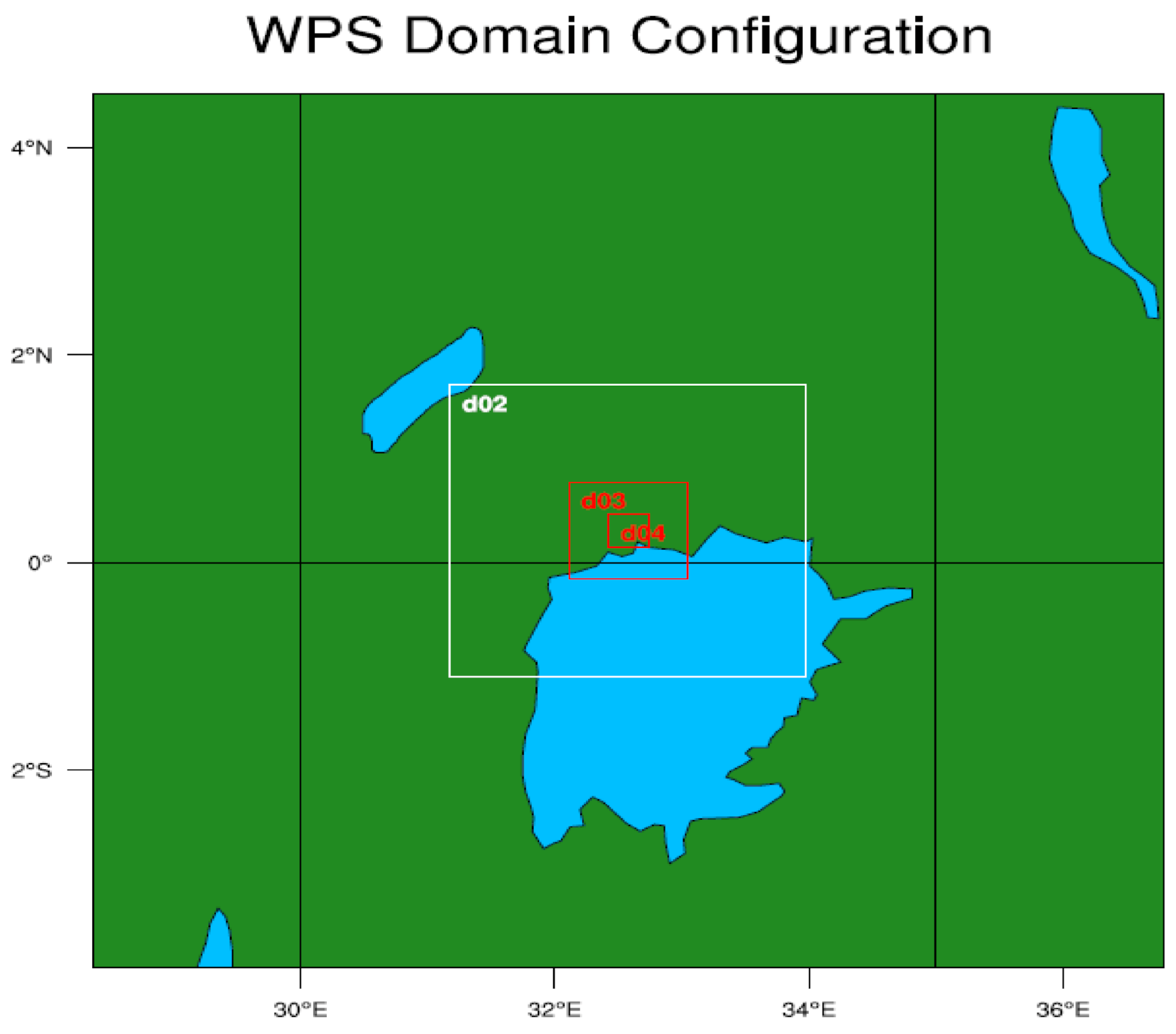
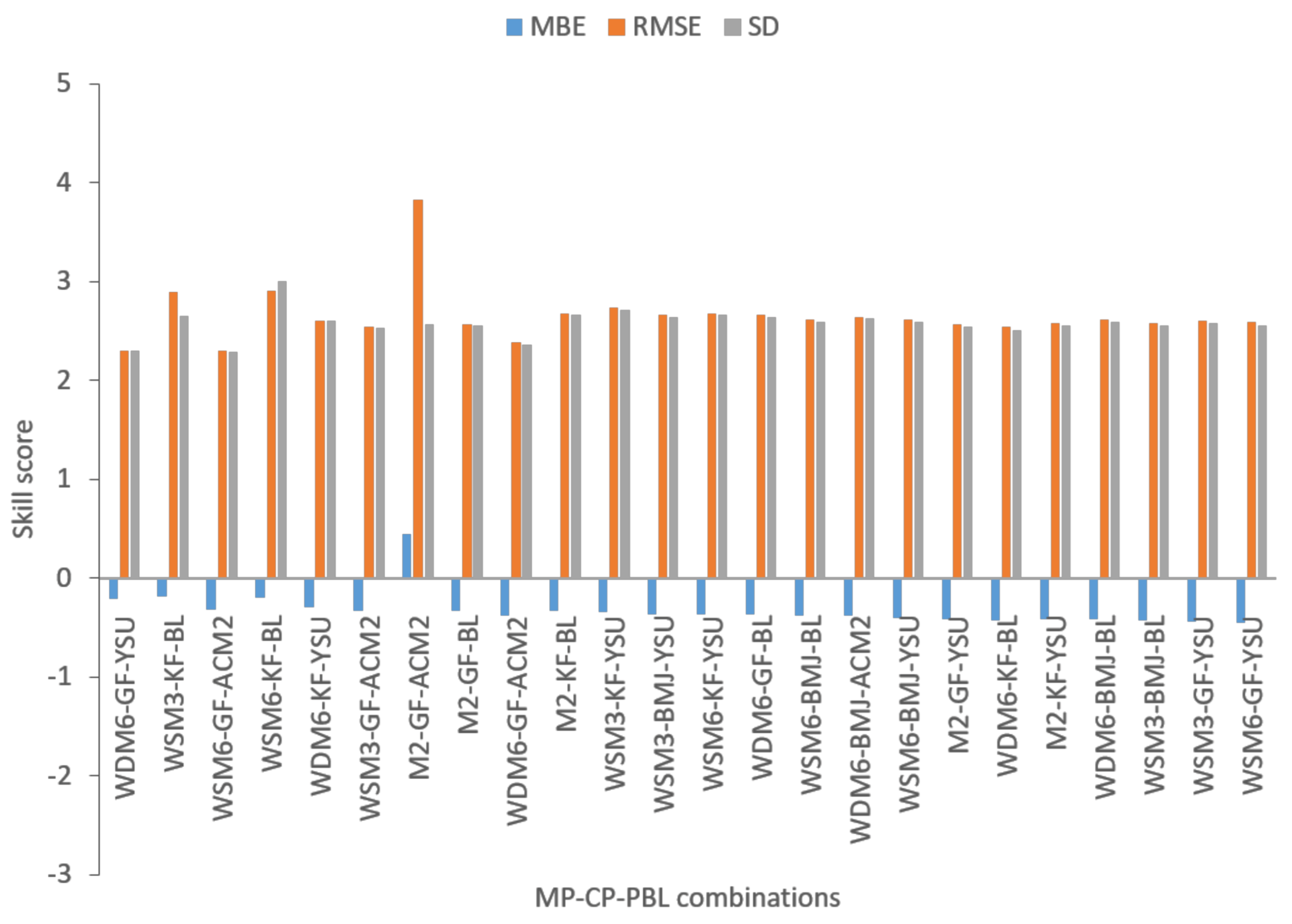
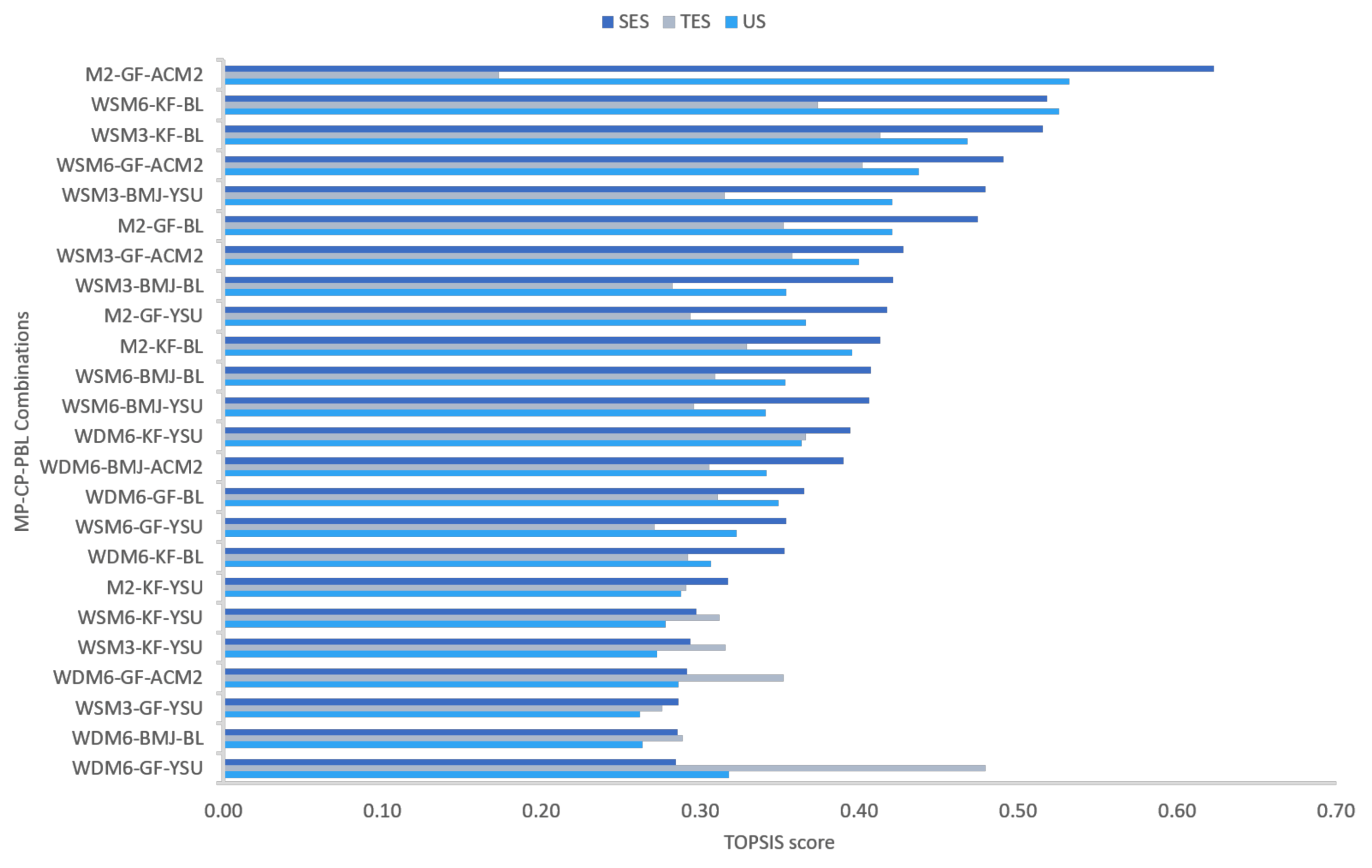
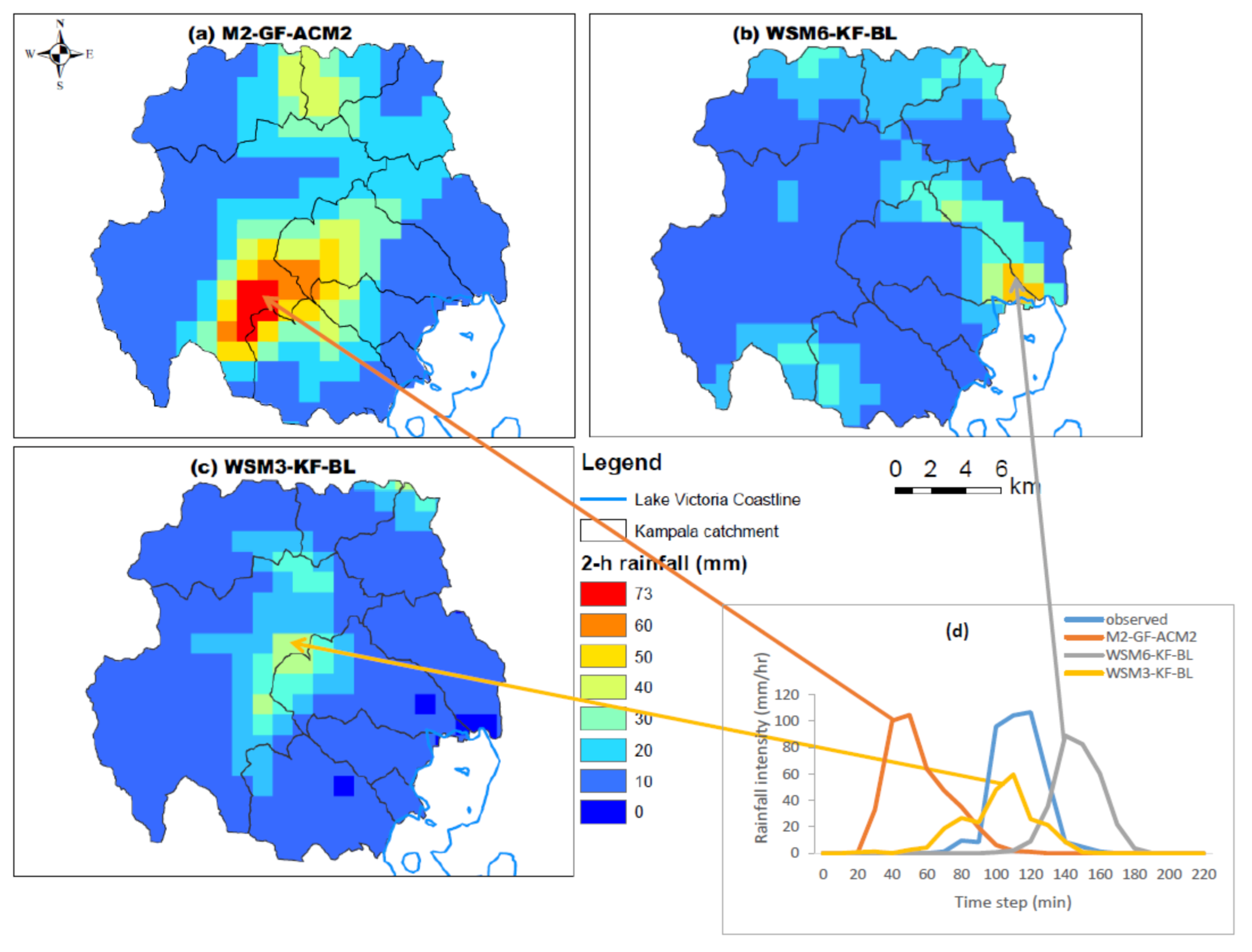
Table 1.
Weather Research and Forecasting (WRF) model settings used in the current study.
| Model | WRF v 4.1 | |||
|---|---|---|---|---|
| Characteristics | Domain 1 (D01) | Domain 2 (D02) | Domain 3 (D03) | Domain 4 (D04) |
| Horizontal grid resolution | 27 km | 9 km | 3 km | 1 km |
| Horizontal Dimensions | 31 × 31 × 31 | 31 × 31 × 31 | 31 × 31 × 31 | 31 × 31 × 31 |
| Time step 60 seconds | adaptive time step | adaptive time step | adaptive time step | adaptive time step |
| Initial-boundary conditions | ERA-5 (30 km) | simulation of domain 1 | simulation of domain 2 | simulation of domain 3 |
| Model run period | 0000 UTC 24 June–1800 UTC 26 June 2012 | |||
Table 2.
WRF parametrization schemes tested in the current study.
| Physics Options | Naming | Description of Parametrization Schemes |
|---|---|---|
| Microphysics scheme (MP) | WSM 3 WSM 5 * | WRF Single Moment 3-class scheme [41] WRF Single Moment 5-class scheme [41] |
| WSM 6 EF * T * | WRF Single Moment 6-class scheme [42] The Eta Ferrier scheme [43] Thomson et al. double moment scheme [44] | |
| M2 WDM 5 * | Morrison et al. 2-Moments scheme [45] WRF Double Moment 5-class scheme [46] | |
| WDM 6 | WRF Double Moment 6-class scheme [46] | |
| Cumulus parametrization (CP) | KF | Kain-Fritsch (new Eta) scheme [47] |
| BMJ | Betts-Miller-Janjic scheme [48] | |
| GF G3D * | Grell-Freitas ensemble scheme [49] Grell 3D ensemble scheme [50] | |
| Planetary Boundary Layer (PBL) | YSU | Yonsei University PBL [51] |
| ACM2 | Asymmetrical Convective Model version 2 PBL [52] | |
| BL | Bougeault-Lacarrere PBL [53] | |
| Radiation-Shortwave | Dudhia | Dudhia Shortwave scheme [54] |
| Radiation-Longwave | RRTM | Rapid Radiative Transfer Model Longwave [55] |
| Land Surface model | NoahMP | Unified Noah land-surface model [56] |
| Surface Layer | SF_SFCLAY | Revised MM5 Monin-Obukhov scheme [57] |
| Urban Physics | SLUCM | Single-layer urban Canopy Model [58] |
* not included in 24 MP-CP-PBL combinations.
Table 3.
Types of indices and their equations used for WRF simulated rainfall evaluation. S and O represent simulated and observed values.
Table 3.
Types of indices and their equations used for WRF simulated rainfall evaluation. S and O represent simulated and observed values.
| Indices Type Formula | Perfect Score | Remark |
|---|---|---|
| Percentage Relative Error (RE%) (1) Root Mean Square Error (RMSE) (2) Mean Bias Error (MBE) (3) Standard Deviation (SD) (4) Probability of detection (POD) (5) Frequency bias index (FBI) (6) False alarm ratio (FAR) (7) Critical success index (CSI) (8) | 0 0 0 0 1 1 0 1 | RE%-calculated using catchment areal 24-hour rainfall of WRF simulated and CHIRPS estimation; measures the relative error of WRF simulated accumulated areal catchment rainfall compared to CHIRPS RMSE-measures the average magnitude error of the WRF simulated rainfall corresponding to the observed rainfall; does not indicate the direction of the deviations. MBE- measures the average cumulative error of the WRF simulated rainfall but does not show the correspondence between the simulation and observation. It also shows the direction of the error whether its negative or positive SD-measures the variation of the overall magnitude of the simulation error due to MBE POD-Indicate what grid rainfall correctly simulated compared the CHIRPS grid rainfall. Sensitivity to the frequency of rainfall occurrence during the event; ignores false alarms. FBI-Indicates the tendency of overestimation (FBI > 1) or underestimation (FBI < 1) of WRF simulated rainfall occurrence FAR-Indicates the grids of the WRF simulated rainfall that have no rainfall compared to the CHIRPS grids. It ignores the misses and sensitive to the frequency of rainfall occurrence during the event CSI-Indicates how the grids rainfall simulated by WRF corresponds to the CHIRPS estimates. It penalizes both misses and false alarms and sensitive to hits |
Table 4.
Contingency table of WRF simulation against CHIRPS rainfall estimates.
| WRF/CHIRPS | RainCHIRPS | No Rain |
|---|---|---|
| RainWRF | RR (hits) | RN (false alarm) |
| No rain | NR (miss) | NN (correct negative) |
Table 5.
Re-scaled indices from the original error indices.
| Rescaled Error Indices | Threshold |
|---|---|
| PODrs = POD | |
| FBIrs = (FBImax − FBI); when FBI > 1 | |
| FBIrs = FBI; when FBI < 1 | |
| FARrs = 1 − FAR | |
| CSIrs = CSI | |
| REr = (1 − RE/REmin); when RE < 0 | REmin = −0.89 |
| RMSErt = (1 − RMSE/RMSEmax) | RMSEmax = 4 |
| MBErt = 1 − MBE/MBEmax; when MBE > 0 | MBEmax = 0.5 |
| MBErt = 1 − MBE/MBEmin; when MBE < 0 | MBEmin = −0.5 |
| SDrt = (1 − SD/Sdmax) | Sdmax = 4 |
| RMSErs = (1 − RMSE/RMSEmax) | RMSEmax = 61 |
| MBErs = 1 − MBE/MBEmax; when MBE > 0 | MBEmax = 61 |
| MBErs = 1 − MBE/MBEmin; when MBE < 0 | MBEmin = −61 |
| SDrs = (1 − SD/Sdmax) | Sdmax = 52 |
The threshold values for RMSEmax, RMSEmin, MBEmax, MBEmin, Sdmax, and Sdmin are in mm.
Table 6.
WRF model performance evaluation of 11 indices and their scores for 24 MP-CP-PBL combinations.
Table 6.
WRF model performance evaluation of 11 indices and their scores for 24 MP-CP-PBL combinations.
| Combinations | Areal Amount | Temporal Dimension | Spatial Dimension Indices | |||||||||
|---|---|---|---|---|---|---|---|---|---|---|---|---|
| Continuous | Categorical | |||||||||||
| Areal (mm) | RE (%) | MBE (mm) | RMSE (mm) | SD(mm) | MBE (mm) | RMSE (mm) | SD (mm) | POD | FBI | FAR | CSI | |
| CHIRPS | 16.8 | |||||||||||
| M2-GF-ACM2 | 16.4 | (−2.4) | 0.44 | 3.82 | 2.56 | 3.39 | 12.37 | 16.99 | 0.35 | 0.41 | 0.14 | 0.33 |
| WSM6-KF-BL | 10.1 | (−39.9) | 0.20 | 2.86 | 2.87 | (−31.43) | 31.50 | 2.99 | 0.30 | 0.40 | 0.25 | 0.27 |
| M2-KF-BL | 8.9 | (−47.0) | (−0.34) | 2.68 | 2.67 | (−48.56) | 48.56 | 0.16 | 0.20 | 0.23 | 0.13 | 0.19 |
| WSM3-GF-ACM2 | 6.7 | (−60.1) | (−0.33) | 2.54 | 2.53 | (−48.94) | 48.96 | 2.22 | 0.30 | 0.60 | 0.49 | 0.23 |
| WSM3-KF-BL | 6.3 | (−62.5) | (−0.19) | 2.89 | 2.65 | (−9.14) | 20.11 | 25.34 | 0.20 | 0.33 | 0.13 | 0.18 |
| WSM6-GF-YSU | 5.7 | (−66.1) | (−0.45) | 2.59 | 2.56 | (−50.24) | 52.28 | 20.44 | 0.24 | 0.32 | 0.23 | 0.23 |
| M2-GF-BL | 5.6 | (−66.7) | (−0.33) | 2.56 | 2.55 | (−49.55) | 49.58 | 2.35 | 0.35 | 0.38 | 0.08 | 0.34 |
| M2-GF-YSU | 5.2 | (−69.0) | (−0.42) | 2.57 | 2.54 | (−57.80) | 57.86 | 3.80 | 0.30 | 0.31 | 0.02 | 0.30 |
| WSM6-GF-ACM2 | 4.3 | (−74.4) | (−0.32) | 2.30 | 2.28 | (−49.60) | 49.68 | 4.05 | 0.40 | 0.43 | 0.07 | 0.39 |
| WDM6-KF-YSU | 3.9 | (−76.8) | (−0.30) | 2.60 | 2.60 | (−49.88) | 50.33 | 9.45 | 0.20 | 0.20 | 0.00 | 0.20 |
| WDM6-BMJ-ACM2 | 3.5 | (−79.2) | (−0.38) | 2.64 | 2.62 | (−54.40) | 54.40 | 1.17 | 0.18 | 0.18 | 0.00 | 0.18 |
| WDM6-GF-BL | 3.5 | (−79.2) | (−0.37) | 2.66 | 2.64 | (-45.89) | 46.50 | 10.63 | 0.13 | 0.16 | 0.15 | 0.13 |
| WSM6-BMJ-BL | 3.5 | (−79.2) | (−0.39) | 2.61 | 2.59 | (−54.40) | 54.41 | 1.53 | 0.25 | 0.29 | 0.12 | 0.25 |
| WSM3-BMJ-YSU | 3.4 | (−79.8) | (−0.36) | 2.66 | 2.64 | (−49.84) | 49.91 | 3.73 | 0.38 | 0.43 | 0.11 | 0.36 |
| WSM3-BMJ-BL | 3.3 | (−80.4) | (−0.43) | 2.58 | 2.55 | (−56.00) | 56.39 | 9.32 | 0.36 | 0.43 | 0.15 | 0.34 |
| M2-KF-YSU | 2.9 | (−82.7) | (−0.42) | 2.58 | 2.55 | (−59.70) | 59.71 | 1.40 | 0.12 | 0.14 | 0.16 | 0.11 |
| WDM6-GF-YSU | 2.9 | (−82.7) | (−0.21) | 2.30 | 2.30 | (−40.70) | 42.18 | 15.67 | 0.05 | 0.12 | 0.56 | 0.05 |
| WDM6-GF-ACM2 | 2.6 | (−84.5) | (−0.38) | 2.38 | 2.36 | (−56.46) | 56.50 | 2.85 | 0.13 | 0.40 | 0.68 | 0.10 |
| WSM3-GF-YSU | 2.5 | (−85.1) | (−0.44) | 2.60 | 2.57 | (−60.73) | 60.78 | 3.44 | 0.15 | 0.30 | 0.52 | 0.14 |
| WSM6-KF-YSU | 2.4 | (−85.7) | (−0.37) | 2.67 | 2.66 | (−55.89) | 55.99 | 4.67 | 0.13 | 0.28 | 0.53 | 0.12 |
| WDM6-BMJ-BL | 2.3 | (−86.3) | (−0.42) | 2.61 | 2.59 | (−57.92) | 57.95 | 2.75 | 0.13 | 0.31 | 0.59 | 0.11 |
| WDM6-KF-BL | 2.2 | (−86.9) | (−0.43) | 2.53 | 2.51 | (−53.60) | 54.26 | 11.96 | 0.16 | 0.16 | 0.01 | 0.16 |
| WSM6-BMJ-YSU | 2.1 | (−87.5) | (−0.41) | 2.62 | 2.59 | (−53.84) | 54.03 | 6.37 | 0.31 | 0.44 | 0.29 | 0.28 |
| WSM3-KF-YSU | 1.8 | (−89.3) | (−0.35) | 2.73 | 2.72 | (−54.81) | 55.04 | 7.18 | 0.11 | 0.20 | 0.42 | 0.11 |
Note: Underlined indicates the top 3 simulations for each index; bold indicates the least performing combination.
Table 7.
Comparison of the combined evaluation index values and their ranks, ranked according to RE score.
Table 7.
Comparison of the combined evaluation index values and their ranks, ranked according to RE score.
| Combinations | RE(%) | TES | SES | US | ||||
|---|---|---|---|---|---|---|---|---|
| Score | Rank | Score | Rank | Score | Rank | Score | Rank | |
| M2-GF-ACM2 | (−2.4) | 1 | 0.36 | 7 | 0.62 | 1 | 0.53 | 1 |
| WSM6-KF-BL | (−39.9) | 2 | 0.37 | 4 | 0.52 | 2 | 0.53 | 2 |
| M2-KF-BL | (−47.0) | 3 | 0.33 | 10 | 0.41 | 10 | 0.30 | 8 |
| WSM3-GF-ACM2 | (−60.1) | 4 | 0.36 | 6 | 0.43 | 7 | 0.40 | 7 |
| WSM3-KF-BL | (−62.5) | 5 | 0.41 | 2 | 0.52 | 3 | 0.47 | 3 |
| WSM6-GF-YSU | (−66.1) | 6 | 0.31 | 13 | 0.35 | 16 | 0.32 | 16 |
| M2-GF-BL | (−66.7) | 7 | 0.35 | 8 | 0.47 | 6 | 0.42 | 6 |
| M2-GF-YSU | (−69.0) | 8 | 0.29 | 18 | 0.42 | 9 | 0.37 | 9 |
| WSM6-GF-ACM2 | (−74.4) | 9 | 0.40 | 3 | 0.49 | 4 | 0.44 | 4 |
| WDM6-KF-YSU | (−76.8) | 10 | 0.37 | 5 | 0.39 | 13 | 0.36 | 10 |
| WDM6-BMJ-ACM2 | (−79.2) | 11 | 0.31 | 16 | 0.39 | 14 | 0.34 | 14 |
| WDM6-GF-BL | (−79.2) | 12 | 0.31 | 14 | 0.37 | 15 | 0.35 | 13 |
| WSM6-BMJ-BL | (−79.2) | 13 | 0.31 | 15 | 0.41 | 11 | 0.35 | 12 |
| WSM3-BMJ-YSU | (−79.8) | 14 | 0.32 | 12 | 0.48 | 5 | 0.42 | 5 |
| WSM3-BMJ-BL | (−80.4) | 15 | 0.28 | 22 | 0.42 | 8 | 0.35 | 11 |
| M2-KF-YSU | (−82.7) | 16 | 0.29 | 20 | 0.32 | 18 | 0.29 | 19 |
| WDM6-GF-YSU | (−82.7) | 17 | 0.48 | 1 | 0.28 | 24 | 0.32 | 17 |
| WDM6-GF-ACM2 | (−84.5) | 18 | 0.35 | 9 | 0.29 | 21 | 0.29 | 20 |
| WSM3-GF-YSU | (−85.1) | 19 | 0.28 | 23 | 0.29 | 22 | 0.26 | 24 |
| WSM6-KF-YSU | (−85.7) | 20 | 0.27 | 24 | 0.30 | 19 | 0.28 | 21 |
| WDM6-BMJ-BL | (−86.3) | 21 | 0.29 | 21 | 0.29 | 23 | 0.26 | 23 |
| WDM6-KF-BL | (−86.9) | 22 | 0.29 | 19 | 0.35 | 17 | 0.31 | 18 |
| WSM6-BMJ-YSU | (−87.5) | 23 | 0.30 | 17 | 0.41 | 12 | 0.34 | 15 |
| WSM3-KF-YSU | (−89.3) | 24 | 0.32 | 11 | 0.20 | 20 | 0.27 | 22 |
Note: Underlined indicates the top 3 simulations for each index; bold indicates the least performing combination.
Table 8.
Comparison of 24-h area-averaged rainfall amount with and without CP in the inner domain and RE calculated with respect to CHIRPS rainfall amount. The number in the square bracket represents the rank.
Table 8.
Comparison of 24-h area-averaged rainfall amount with and without CP in the inner domain and RE calculated with respect to CHIRPS rainfall amount. The number in the square bracket represents the rank.
| CP-on | CP-off | (CP-on)–(CP-off) | |||
|---|---|---|---|---|---|
| MP-CP-PBL Combinations | Area Average Rainfall (mm) | RE(%) | Area Average Rainfall (mm) | RE(%) | Difference (mm) |
| CHIRPS | 16.8 | ||||
| M2-GF-ACM2 | 16.4 | (−2.4) [1] | 16 | (−4.8) [1] | 0.4 |
| WSM6-KF-BL | 10.1 | (−39.9) [2] | 9.8 | (−41.7) [7] | 0.3 |
| M2-KF-BL | 8.9 | (−47.0) [3] | 1.8 | (−89.3) [18] | 7.1 |
| WSM3-GF-ACM2 | 6.7 | (−60.1) [4] | 6.1 | (−63.7) [13] | 0.6 |
| WSM3-KF-BL | 6.3 | (−62.5) [5] | 3.5 | (−79.2) [15] | 2.8 |
| WSM6-GF-YSU | 5.7 | (−66.1) [6] | 0.3 | (−98.2) [22] | 5.4 |
| M2-GF-BL | 5.6 | (−66.7) [7] | 7.7 | (−54.2) [9] | (−2.1) |
| M2-GF-YSU | 5.2 | (−69.0) [8] | 6.7 | (−60.1) [11] | (−1.5) |
| WSM6-GF-ACM2 | 4.3 | (−74.4) [9] | 10.3 | (−38.7) [6] | (−6) |
| WDM6-KF-YSU | 3.9 | (−76.8) [10] | 2.4 | (−85.7) [16] | 1.5 |
| WDM6-BMJ-ACM2 | 3.5 | (−79.2) [11] | 1.7 | (−89.9) [19] | 1.8 |
| WDM6-GF-BL | 3.5 | (−79.2) [12] | 1.5 | (−91.1) [20] | 2 |
| WSM6-BMJ-BL | 3.5 | (−79.2) [13] | 10.4 | (−38.1) [5] | (−6.9) |
| WSM3-BMJ-YSU | 3.4 | (−79.8) [14] | 8.4 | (−50.0) [8] | (−5) |
| WSM3-BMJ-BL | 3.3 | (−80.4) [15] | 4.8 | (−71.4) [14] | (−1.5) |
| M2-KF-YSU | 2.9 | (−82.7) [16] | 6.6 | (−60.7) [12] | (−3.7) |
| WDM6-GF-YSU | 2.9 | (−82.7) [17] | 0 | (−100.0) [24] | 2.9 |
| WDM6-GF-ACM2 | 2.6 | (−84.5) [18] | 13.2 | (−21.4) [3] | (−10.6) |
| WSM3-GF-YSU | 2.5 | (−85.1) [19] | 7.1 | (−57.7) [10] | (−4.6) |
| WSM6-KF-YSU | 2.4 | (−85.7) [20] | 1.9 | (−88.7) [17] | 0.5 |
| WDM6-BMJ-BL | 2.3 | (−86.3) [21] | 10.9 | (-35.1) [4] | (−8.6) |
| WDM6-KF-BL | 2.2 | (−86.9) [22] | 1 | (−94.0) [21] | 1.2 |
| WSM6-BMJ-YSU | 2.1 | (−87.5) [23] | 15.1 | (−10.1) [2] | (−13) |
| WSM3-KF-YSU | 1.8 | (−89.3) [24] | 0.1 | (−99.4) [23] | 1.7 |
Publisher’s Note: MDPI stays neutral with regard to jurisdictional claims in published maps and institutional affiliations. |
© 2021 by the authors. Licensee MDPI, Basel, Switzerland. This article is an open access article distributed under the terms and conditions of the Creative Commons Attribution (CC BY) license (http://creativecommons.org/licenses/by/4.0/).
Share and Cite
MDPI and ACS Style
Umer, Y.; Ettema, J.; Jetten, V.; Steeneveld, G.-J.; Ronda, R. Evaluation of the WRF Model to Simulate a High-Intensity Rainfall Event over Kampala, Uganda. Water 2021, 13, 873. https://doi.org/10.3390/w13060873
AMA Style
Umer Y, Ettema J, Jetten V, Steeneveld G-J, Ronda R. Evaluation of the WRF Model to Simulate a High-Intensity Rainfall Event over Kampala, Uganda. Water. 2021; 13(6):873. https://doi.org/10.3390/w13060873
Chicago/Turabian StyleUmer, Yakob, Janneke Ettema, Victor Jetten, Gert-Jan Steeneveld, and Reinder Ronda. 2021. "Evaluation of the WRF Model to Simulate a High-Intensity Rainfall Event over Kampala, Uganda" Water 13, no. 6: 873. https://doi.org/10.3390/w13060873
Note that from the first issue of 2016, this journal uses article numbers instead of page numbers. See further details here.